Channel-wise and Spatial Feature Modulation Network for Single Image Super-Resolution

Abstract

The performance of single image super-resolution has achieved significant improvement by utilizing deep convolutional neural networks (CNNs). The features in deep CNN contain different types of information which make different contributions to image reconstruction. However, most CNN-based models lack discriminative ability for different types of information and deal with them equally, which results in the representational capacity of the models being limited. On the other hand, as the depth of neural networks grows, the long-term information coming from preceding layers is easy to be weaken or lost in late layers, which is adverse to super-resolving image. To capture more informative features and maintain long-term information for image super-resolution, we propose a channel-wise and spatial feature modulation (CSFM) network in which a sequence of feature-modulation memory (FMM) modules is cascaded with a densely connected structure to transform low-resolution features to high informative features. In each FMM module, we construct a set of channel-wise and spatial attention residual (CSAR) blocks and stack them in a chain structure to dynamically modulate multi-level features in a global-and-local manner. This feature modulation strategy enables the high contribution information to be enhanced and the redundant information to be suppressed. Meanwhile, for long-term information persistence, a gated fusion (GF) node is attached at the end of the FMM module to adaptively fuse hierarchical features and distill more effective information via the dense skip connections and the gating mechanism. Extensive quantitative and qualitative evaluations on benchmark datasets illustrate the superiority of our proposed method over the state-of-the-art methods.

I Introduction

Single image super-resolution (SISR), which aims at reconstructing a high-resolution (HR) image from its single low-resolution (LR) counterpart, is an ill-posed inverse problem. To tackle such an inverse problem, numerous learning-based super-resolution (SR) methods have been proposed to learn the mapping function between LR and HR image pairs via probabilistic graphical model [1, 2], neighbor embedding [3, 4], sparse coding [5, 6], linear or nonlinear regression [7, 8, 9], and random forest [10].

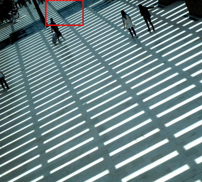
(a) “img093” from Urban100 [11]

(b) Ground Truth
PSNR / SSIM

(c) Bicubic23.63dB / 0.8041

(d) EDSR [12]
29.56dB / 0.9336

(e) RDN [13]
28.59dB / 0.9286

(f) CSFM(ours)
32.06dB / 0.9462

Figure 1: The comparisons of our proposed method (CSFM) with existing methods on single image super-resolution for a scale factor of $4\times$. Our proposed CSFM network generates more realistic visual result.

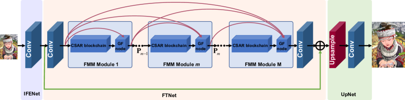
(a) The architecture of the proposed CSFM network

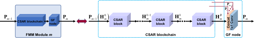
(b) The structure of feature-modulation memory (FMM) module in CSFM network

Figure 2: The architecture of our CSFM network and the structure of FMM module in CSFM network. (a) The overall architecture of the proposed CSFM network, which adopts adaptive feature-modulation strategy, long-term information persistence mechanism and post-upscaling scheme to boost SR performance. (b) The feature-modulation memory (FMM) module in (a), which exploits a chain of channel-wise and spatial attention residual (CSAR) blocks to capture more informative features and utilizes the gated fusion (GF) node to fusion long-term information from the preceding FMM modules and short-term information from the current module.

More recently, benefiting from the powerful representational ability of convolutional neural networks (CNNs), deep-learning-based SR methods have achieved better performances in terms of effectiveness and efficiency. As an early first attempt, SRCNN [14] proposed by Dong et al. employed three convolutional layers to predict the nonlinear mapping function from bicubic upscaled middle resolution image to high resolution image, which outperformed most conventional SR methods. Later, various works followed the similar network design and consistently improved SR performance via residual learning [15, 16], recursive learning [16, 17], symmetric skip connections [18] and cascading memory blocks [19]. Differing from the above pre-upscaling approaches which operated SR on bicubic upsampled images, FSRCNN [20] and ESPCN [21], designed by Dong et al. and Shi et al. respectively, extracted features from the original LR images and upsampled spatial resolution only at the end of the processing pipeline via a deconvolution layer or a sub-pixel convolution module [21]. Following this post-upscaling architecture, Ledig et al. [22] employed the residual blocks proposed in [23] to construct a deeper network (SRResnet) for image SR, which was further improved by EDSR [12] and MDSR [12] via removing unnecessary modules. Further, to conveniently pass information across several layers, dense blocks [24] were also introduced to construct several deep networks [25, 13, 26] for suiting image super-resolution. Meanwhile, to simplify the difficulty of direct super-resolving the details, [26, 27, 28] adopted the progressive structure to reconstruct HR image in a stage-by-stage upscaling manner. In addition, [29, 30] incorporated the feedback mechanism into network designs for exploiting both LR and HR signals jointly.

Although these existing deep-learning-based approaches have made good efforts to improve SR performance, the reconstruction of high frequency details for SISR is still a challenge. In deep neural networks, the LR inputs and extracted features contain different types of information across channels, spaces and layers, such as low-frequency and high-frequency information or low-level and high-level features, which have different reconstruction difficulties (e.g., the high-frequency features or the pixels on the texture areas are more difficult to reconstruction than the low-frequency features or the pixels on the flat areas) as well as different contributions to recovering the implicit high-frequency details. However, the most CNN-based methods consider different types of information equally and lack flexible modulation ability in dealing with them, which resultantly limits the representational ability and fitting capacity of the deep networks. Therefore, for the deeper neural networks, simply increasing depth or width can hardly achieve better improvement. On the other hand, for image restoration tasks, the hierarchical features produced by deep neural networks are informative and useful. However, many very deep networks, such as VDSR [15], LapSRN [27], EDSR [12] and IDN [31], adopt single-path direct connections or short skip connections among layers, where hierarchical features could hardly be fully utilized and long-term information that provides some clues for SR would be lost as the network depth grows. Although SRDenseNet [25] and RDN [13] employ dense-connection blocks for SR to fuse different levels of features, the extreme connectivity pattern in their networks not only hinders their scalability to large width or high depth but also produces redundant computation. Memory blocks adopted in MemNet [19] also integrate information from the preceding memory blocks to achieve persistent memory, but the fused features are extracted from bicubic pre-upscaled images which might lose some details and produce new noises. Therefore, how to effectively make full use multi-level, channel-wise and spatial features within neural networks is crucial for HR image reconstruction and remains to be explored.

To address these issues, we propose a Channel-wise and Spatial Feature Modulation network (illustrated in Fig. 2) for SISR, named CSFM, which not only adaptively learns to pay attention to every feature entry in the multi-level, channel-wise and spatial feature responses but also fully and effectively exploits the hierarchical features to maintain persistent memory. In the CSFM network, we construct a feature-modulation memory (FMM) module (shown in Fig. 2(b)) as the building module and stack several FMM modules with a densely connected structure. An FMM module contains a channel-wise and spatial attention residual (CSAR) blockchain and a gated fusion (GF) node. In the CSAR blockchain, we develop a channel-wise and spatial attention residual (CSAR) block via integrating the channel-wise and spatial attentions into the residual block [23] and stack a collection of CSAR blocks to modulate multi-level features for adaptively capturing more important information. In addition, by adopting a GF node in the FMM module, the states of the current FMM module and of the preceding FMM modules are conveniently concatenated and adaptively fused for short-term and long-term information preservation as well as for information flow enhancement. As shown in Fig. 1, our proposed CSFM network generates more realistic visual result compared with other methods.

In summary, the major contributions of our proposed SISR method are three-fold:

1). We develop a CSAR block via combining channel-wise and spatial attention mechanisms into the residual block, which can adaptively recalibrate the feature responses in a global-and-local manner by explicitly modelling channel-wise and spatial feature interdependencies.

2). We construct an FMM module via stacking a set of CSAR blocks to modulate multi-level features and adding a GF node to adaptively fuse hierarchical features for important information preservation. The block-stacking structure in the FMM module enables it to capture different types of attention and then enhance high contribution information for image super-resolution, while the gating mechanism help it to adaptively distill more effective information from short-term and long-term states.

3) We design a CSFM network for accurate single image SR, in which the stacked FMM modules enhance discriminative learning ability of the network and the densely connected structure helps to fully exploit multi-level information as well as ensures maximum information flow between modules.

The remainder of this paper is organized as follows. Section II discusses the related SISR methods and correlative mechanisms applied in neural networks. Section III describes the proposed CSFM network for SR in detail. Model analysis and experimental comparisons with other state-of-the-art methods are presented in Section IV, and Section V concludes the paper with observations and discussions.

II Related Work

Numerous SISR methods, different learning mechanisms and various network architectures have been proposed in the literatures. Here, we focus our discussions on the approaches which are related to our method.

II-A Deep-learning based Image Super-Resolution

Since Dong et al. [10] first proposed a super-resolution convolutional neural network (SRCNN) to predict the nonlinear relationship between bicubic upscaled image and HR image, various CNN architectures have been studied for SR. As deeper CNNs have larger receptive fields to capture more contextual information, Kim et al. proposed two deep networks of VDSR [15] and DRCN [17] which utilized global residual learning and recursive layers respectively to improve SR accuracy. To control the number of model parameters and maintain persistent memory, Tai et al. constructed the recursive blocks with global-and-local residual learning in DRRN [16] and designed the memory blocks with dense connections in MemNet [19]. For these methods, the LR images need be bicubic interpolated to the desired size before entering the networks, which inevitably increases the computational complexity and might produce new noise.

For alleviating the computational loads and overcoming the disadvantage of the pre-upscaling structure, Dong et al. [20] exploited the deconvolution operator to upscale spatial resolution at the network tail. Later, Shi et al. [21] proposed a more effective sub-pixel convolution layer to replace the deconvolution layer for upscaling the final LR feature-maps into the HR output, which was recently extended by an enhanced upscaling module (EUM) [32] via applying residual learning and multi-path concatenation into the module. Benefiting from this post-upscaling strategy, more and more deeper networks, such as SRResnet [22], EDSR [12] and SRDenseNet [25], achieved high performances with less computational load. Recently, Hui et al. [31] developed the information distillation blocks and stacked them to construct a deep and compact convolutional network. And, Zhang et al. [13] proposed a residual dense network (RDN) which used the densely connected convolutional layers to extract abundant local features and adopted the local-and-global feature fusion procedure to adaptively fuse hierarchical features in the LR space.

Taking the effectiveness of post-upscaling strategy into account, we also apply the sub-pixel convolution layer [21] at the end of network for upscaling spatial resolution. Furthermore, we exploit the feature modulation mechanism to enhance the discriminative ability of the network for different types of information.

II-B Attention Mechanism

The aim of attention mechanism in neural network is to recalibrate the feature responses towards the most informative and important components of the inputs. Recently, some works have focused on the integration of attention modules within deep network architectures on a range of tasks, such as image generation [33], image captioning [34, 35], image classification [36, 37] and image restoration [38, 39]. Xu et al. [34] proposed a visual attention model for image captioning, which used hard pooling to select the most probably attentive region or soft pooling to average the spatial features with attentive weights. Xu et al. [40] further refined the spatial attention model by stacking two spatial attention models for visual question answering. Moreover, by investigating the interdependencies between the channels of the convolutional features in a network, Hu et al. [36] introduced a channel-wise attention mechanism and proposed a squeeze-and-excitation (SE) block to adaptively recalibrate channel-wise feature responses for image classification. Recently, inspired by SE networks, Zhang et al. [38] integrated the channel-wise attention into the residual blocks and proposed a very deep residual channel attention network which pushed the state-of-the-art performance of SISR forward. In addition, Chen et al. [35] stacked the spatial and channel-wise attention modules at multiple layers for image captioning, where the second attention (spatial attention or channel-wise attention) was operated on the attentive feature-maps recalibrated by the first one (channel-wise attention or spatial attention). Besides the spatial and channel-wise attentions, Wang et al. [39] utilized semantic segmentation probability maps as prior knowledge and introduced semantic attention to modulate spatial features for realistic texture generation. However, this model requires external resources to train these semantic attributes.

Inspired by attention mechanism and considering that there are different types of information within and across feature-maps which have different contributions for image SR, we combine channel-wise and spatial attentions into the residual blocks to adaptively modulate feature representations in a global-and-local way for capturing more important information.

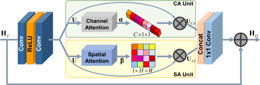
(a) Channel-wise and spatial attention residual (CSAR) block

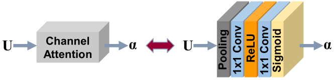
(b) The operations of channel-wise attention

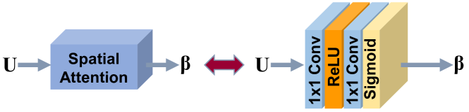
(c) The operations of spatial attention

Figure 3: The diagram of channel-wise and spatial attention residual (CSAR) block, where $\bigotimes$ denotes element-wise product. (a) The CSAR block, which integrates the channel-wise attention and spatial attention into the residual block to modulate the residual features. (b) The operations of channel-wise attention, including global-pooling, convolutions and activations, by which the channel-wise attention weights are calculated. (c) The operations of convolutions and activations in spatial attention by which the spatial attention mask is generated.

II-C Skip Connections

As the depth of a network grows, the problems of information flow weakened and gradient vanishing hamper the training of the network. Many recent methods have been devoted to resolving these problems. ResNets proposed by He et al. [23] was built by stacking a sequence of residual blocks, which utilized the skip connections between layers to improve information flow and make training easier. The residual blocks were also widely applied in [22, 12] to construct very wide and deep networks for SR performance improvement. To fully explore the advantages of skip connections, Huang et al. [24] constructed DenseNets by directly connecting each layer to all previous layers. Meanwhile, in order to make the networks scale to deep and wide ones, block compression was applied in DenseNets to halve the number of channels in the concatenation of previous layers. The dense connections were utilized in [19, 25, 13] for image SR to improve the flows of information and gradient throughout the networks as well. However, the extremely dense connections and frequent concatenations may increase information redundancy and computational cost. Considering these, Chen et al. [41] combined the insights of ResNets [23] and DenseNets [24] and proposed a DualPathNet which utilized both concatenation and summation for previous features.

Recognizing both advantages of residual path in residual block and densely connected paths in dense block, we stack several attention-based residual blocks within each module and utilize the densely connected paths between modules for effective feature re-exploitation and important information preservation.

III The Proposed CSFM Network

The proposed CSFM network for SISR, outlined in Fig. 2, consists of an initial feature extraction sub-network (IFENet), a feature transformation sub-network (FTNet) and an upscaling sub-network (UpNet). The IFENet is applied to represent a LR input as a set of feature-maps via a convolutional layer. The FTNet is designed to capture more informative features for SR by a sequence of stacked feature-modulation memory (FMM) modules and two convolutional layers. The transformed features are then fed into the UpNet to generate the HR image. In this section, we detail the proposed model, from the channel-wise and spatial attention residual (CSAR) block to the FMM module and finally the overall network architecture.

III-A The CSAR Block

The features generated by a deep network contain different types of information across channels and spatial regions which have different contributions for the high-frequency details recovery. If we are able to increase the network’s sensitivity to higher contribution features and make it focus on learning more important features, the representational power of the network would be enhanced and the performance improved. Keeping that in mind, we design a channel-wise attention (CA) unit and a spatial attention (SA) unit by utilizing the interdependencies between channels and spatial locations of the features, and then combine two types of attention into the residual blocks to adaptively modulate feature representations.

III-A1 The CA Unit

The aim of the CA unit is to perform feature recalibration in a global way where the per-channel summary statistics are calculated and then used to selectively emphasis informative feature-maps as well as suppress useless ones (e.g. redundant feature-maps). The structure of the CA unit is illustrated in Fig. 3(a)–(b). We denote $\mathbf{U}=\left[{{\mathbf{u}}_{1}},{{\mathbf{u}}_{2}},\cdots,{{\mathbf{u}}_{C}}\right]$ as the input of the CA unit, which consists of $C$ feature-maps with size of $H\times W$. To generate channel-wise summary statistics $\mathbf{z}\in{{\mathbb{R}}^{C\times 1\times 1}}$, the global average pooling is operated on individual feature channels across spatial dimensions $H\times W$, as done in [36]. The $c\text{-th}$ element of $\mathbf{z}$ is computed by

$${{z}_{c}}=\frac{1}{H\times W}\sum\limits_{i=1}^{H}{\sum\limits_{j=1}^{W}{{{\mathbf{u}}_{c}}(i,j)}},$$ (1)

where ${{\mathbf{u}}_{c}}(i,j)$ is the value at position $\left(i,j\right)$ of the $c\text{-th}$ channel ${{\mathbf{u}}_{c}}$. To assign different attentions to different types of feature-maps, we employ a gating mechanism with a sigmoid activation to summary statistic $\mathbf{z}$. The process is represented as follows.

$$\bm{\upalpha}=\sigma(\mathbf{W}_{CA}^{2}*\delta(\mathbf{W}_{CA}^{1}*\mathbf{z}+\mathbf{b}_{CA}^{1})+\mathbf{b}_{CA}^{2}),$$ (2)

where $\sigma\left(\cdot\right)$ and $\delta\left(\cdot\right)$ represent the sigmoid and ReLU [42] functions respectively, and $*$ denotes the convolution operation. $\mathbf{W}_{CA}^{1}\in{{\mathbb{R}}^{\frac{C}{r}\times C\times 1\times 1}}$ and $\mathbf{b}_{CA}^{1}\in{{\mathbb{R}}^{\frac{C}{r}}}$ are the weights and bias in the first convolutional layer which is followed by ReLU activation and used to decrease the number of channels of $\mathbf{z}$ by the reduction ratio $r$. Next, the number of channels is increased back to the original amount via another convolutional layer with parameters of $\mathbf{W}_{CA}^{2}\in{{\mathbb{R}}^{C\times\frac{C}{r}\times 1\times 1}}$ and $\mathbf{b}_{CA}^{2}\in{{\mathbb{R}}^{C}}$. In addition, the channel-wise attention weights $\bm{\upalpha}\in{{\mathbb{R}}^{C\times 1\times 1}}$ are adapted to the values between $0$ and $1$ by sigmoid function $\sigma\left(\cdot\right)$, and then used to rescale the input features as follows.

$${{\mathbf{U}}_{CA}}={{\Phi}_{CA}}(\mathbf{U})={{f}_{CA}}(\mathbf{U},\bm{\upalpha}),$$ (3)

where ${{f}_{CA}}\left(\cdot\right)$ is a channel-wise multiplication for feature channels and corresponding channel weights, ${\mathbf{U}}_{CA}$ is the channel-wise recalibrated output, and ${{\Phi}_{CA}}(\cdot)$ represents the CA unit which is apparently conditioned on the input $\mathbf{U}$.

With the above process, the CA unit is able to adaptively modulate the channel-wise features according to the channel-wise statistics of input, and help the network boost the channel-wise feature discriminability.

III-A2 The SA Unit

The channel-wise attention exploits global average pooling to squeeze global spatial information into a channel statistical descriptor, by which the spatial information within each feature-map is yet removed. On the other hand, the information contained in the inputs and feature-maps is also diverse over spatial positions. For example, the edge or texture regions usually contain more high-frequency information while the smooth areas have more low-frequency information. Therefore, to recover high-frequency details for image SR, it is helpful to make the network have discriminative ability for different local regions and pay more attentions to the regions which are more important and more difficult to reconstruct.

Considering aforementioned discussion, besides the channel-wise attention, we explore a complementary form of attention termed as spatial attention to improve the representations of the network. As shown in Fig. 3(a)–(c), let $\mathbf{U}=\left[{{\mathbf{u}}_{1}},{{\mathbf{u}}_{2}},\cdots,{{\mathbf{u}}_{C}}\right]$ be an input for the SA unit, which has $C$ feature-maps with size of $H\times W$. To make use of feature channel interdependencies of the input and inspired by the local computations in computational-neuroscience models [43], we use a two-layers neural network followed by a sigmoid function to generate a spatial attention mask $\bm{\upbeta}\in{{\mathbb{R}}^{1\times H\times W}}$. Below is the definition of the SA unit.

$$\bm{\upbeta}=\sigma(\mathbf{W}_{SA}^{2}*\delta(\mathbf{W}_{SA}^{1}*\mathbf{U}+\mathbf{b}_{SA}^{1})+\mathbf{b}_{SA}^{2}),$$ (4)

where the meanings of the notations $\sigma\left(\cdot\right)$, $\delta\left(\cdot\right)$ and $*$ are the same as those used in Eq. (2). The first convolutional layer with parameters of $\mathbf{W}_{SA}^{1}\in{{\mathbb{R}}^{\gamma C\times C\times 1\times 1}}$ and $\mathbf{b}_{SA}^{1}\in{{\mathbb{R}}^{\gamma C}}$ is used to yield per-channel attentive maps which are then combined into a single attentive map by the second $1\times 1$ convolutional layer (parameterized by $\mathbf{W}_{SA}^{2}$ and $\mathbf{b}_{SA}^{2}$). Further, the sigmoid function $\sigma\left(\cdot\right)$ normalizes the attentive map range to $\left[0,1\right]$ to obtain the spatial attention soft mask $\bm{\upbeta}$. The process of input features being spatially modulated by $\bm{\upbeta}$ can be formulated as

$${{\mathbf{U}}_{SA}}={{\Phi}_{SA}}(\mathbf{U})={{f}_{SA}}(\mathbf{U},\bm{\upbeta}),$$ (5)

where ${{f}_{SA}}\left(\cdot\right)$ is an element-wise multiplication for spatial positions of each feature-map and their corresponding spatial attention weights, and ${{\Phi}_{SA}}\left(\cdot\right)$ denotes the SA model.

With the SA unit, the features are adaptively modulated in a local way, which could be interplayed with the global channel-wise modulation to help the network enhancing the representational power.

III-A3 Integration of CA and SA into the Residual Block

Since the residual blocks introduced in ResNets [23] can improve information flow and achieve better performance for image SR in [12], we combine the channel-wise and spatial attention units into the residual block and propose the CSAR block.

As illustrated in Fig. 3, if we denote ${{\mathbf{H}}_{I}}$ and ${{\mathbf{H}}_{O}}$ as the input and output of a CSAR block, and ${{\Phi}}\left(\cdot\right)$ as the combinational attention model of CA and SA that will be detailed later, the CSAR block can be formulated as

$${{\mathbf{H}}_{O}}={\mathcal{Q}}({{\mathbf{H}}_{I}})={{\mathbf{H}}_{I}}+{\Phi}\left(\mathbf{U}\right)={{\mathbf{H}}_{I}}+\Phi\left({\mathcal{R}}({{\mathbf{H}}_{I}})\right),$$ (6)

where ${\mathcal{Q}}\left(\cdot\right)$ and ${\mathcal{R}}\left(\cdot\right)$ represent the functions of the CSAR block and the residual branch respectively. The residual branch contains two stacked convolutional layers with a ReLU activation,

$$\mathbf{U}={\mathcal{R}}({{\mathbf{H}}_{I}})=\mathbf{W}_{{\mathcal{R}}}^{2}*\delta(\mathbf{W}_{{\mathcal{R}}}^{1}*{{\mathbf{H}}_{I}}+\mathbf{b}_{{\mathcal{R}}}^{1})+\mathbf{b}_{{\mathcal{R}}}^{2},$$ (7)

where $\left\{\mathbf{W}_{{\mathcal{R}}}^{i}\right\}_{i=1}^{2}$ and $\left\{\mathbf{b}_{{\mathcal{R}}}^{i}\right\}_{i=1}^{2}$ are the weight and bias sets of the residual branch and $\mathbf{U}$ is a set of produced residual features.

To capture more important information, we apply the combinational attention model ${{\Phi}}\left(\cdot\right)$ to modulate the residual features $\mathbf{U}$. At first, we operate the CA unit ${{\Phi}_{CA}}\left(\cdot\right)$ and the SA unit ${{\Phi}_{SA}}\left(\cdot\right)$ on the residual features $\mathbf{U}$ respectively to obtain channel-wise weighted feature-maps ${{\mathbf{U}}_{CA}}$ and spatial weighted feature-maps ${{\mathbf{U}}_{SA}}$, as described in Section III. A 1) and 2). Then, two sets of modulated feature-maps are concatenated as the input to a $1\times 1$ convolutional layer ( parameterized by ${{\mathbf{W}}_{\Phi}}$ and ${{\mathbf{b}}_{\Phi}}$ ) which is utilized to fuse two types of attention-modulated features with learned adaptive weights. All processes are summarized as follows.

$$\begin{split}&{{\mathbf{U}}_{CA}}={{\Phi}_{CA}}\left(\mathbf{U}\right),\\ &{{\mathbf{U}}_{SA}}={{\Phi}_{SA}}\left(\mathbf{U}\right),\\ &\Phi\left(\mathbf{U}\right)={{\mathbf{W}}_{\Phi}}*\left[{{\mathbf{U}}_{CA}},{{\mathbf{U}}_{SA}}\right]+{{\mathbf{b}}_{\Phi}},\end{split}$$ (8)

where $\left[\cdot\right]$ represents the operation of feature concatenation.

Inserting the combinational attention model into the deep network in the way described above has two benefits. First, since the combinational attention model only modulates the residual features, the good property of the identical mapping in the residual block is not broken and the information flow is still improved. Second, as two attention units are combined into a residual block, we can conveniently apply channel-wise and spatial attentions to multi-level features by stacking multiple CSAR blocks, and thus more multi-level important information is captured.

III-B The FMM Module

To make full use of the attention mechanism and conveniently maintain persistent memory, the FMM module is built. As illustrated in Fig. 2(b), the FMM module contains a CSAR blockchain and a gated fusion (GF) node.

The CSAR blockchain is constructed by stacking multiple CSAR blocks in a chain structure, which is exploited to perform channel-wise and spatial feature modulation at multiple levels. Supposing $B$ CSAR blocks in a blockchain are stacked in sequence, the input of the first CSAR block ${{\mathbf{H}}^{0}}$ and the output of the last CSAR block ${{\mathbf{H}}^{B}}$ are obviously the input and output of the CSAR blockchain. Thus, the CSAR blockchain can be formulated as below.

$${{\mathbf{H}}^{B}}={} {\mathcal{Q}}^{(B)}({{\mathbf{H}}^{0}})$$ (9)

$$={} {\mathcal{Q}}^{B}\left({\mathcal{Q}}^{B-1}\left(\cdots\left({\mathcal{Q}}^{1}({{\mathbf{H}}^{0}})\right)\cdots\right)\right),$$

where $\left\{{\mathcal{Q}}^{b}\left(\cdot\right)\right\}_{b=1}^{B}$ are the functions for the CSAR blocks as depicted in Eq. (6), and ${\mathcal{Q}}^{(B)}(\cdot)$ denotes the operation of the CSAR blockchain.

To preserve long-term information when multiple FMM modules are stacked in the deep network, the GF node is attached to integrate the information coming from the previous FMM modules and from the current blockchain through an adaptive learning process. In the GF node, the features generated by the preceding FMM modules and by the current CSAR blockchain are firstly concatenated and then fed into a convolutional layer to be adaptively fused. Let ${{\mathbf{P}}_{i}}(i=1,2,\cdots,m-1)$ and $\mathbf{H}_{m}^{B}$ be the output features of $m-1$ previous FMM modules and of the current CSAR blockchain with $B$ CSAR blocks. The process of gated fusion is formulated as

$${{\mathbf{P}}_{m}}={} {{\phi}_{m}}([\mathbf{H}_{m}^{B},{{\mathbf{P}}_{1}},{{\mathbf{P}}_{2}},\cdots,{{\mathbf{P}}_{m-1}}])$$ (10)

$$={} \mathbf{W}_{GF}^{m}*\left[\mathbf{H}_{m}^{B},{{\mathbf{P}}_{1}},{{\mathbf{P}}_{2}},\cdots,{{\mathbf{P}}_{m-1}}\right]+\mathbf{b}_{GF}^{m},$$

where ${{\phi}_{m}}\left(\cdot\right)$ denotes the function of the $1\times 1$ convolutional layer with parameters of ${\mathbf{W}_{GF}^{m}}$ and ${\mathbf{b}_{GF}^{m}}$. This convolutional layer accomplishes the gating mechanism to learn adaptive weights for different information and then controls the output information. Based on those depicted above, the formulation of the $m\text{-th}$ FMM module can be written as

$${{\mathbf{P}}_{m}}={} {{\mathcal{G}}_{m}}({{\mathbf{P}}_{m-1}})={{\phi}_{m}}([\mathbf{H}_{m}^{B},{{\mathbf{P}}_{1}},{{\mathbf{P}}_{2}},\cdots,{{\mathbf{P}}_{m-1}}])$$ (11)

$$={} {{\phi}_{m}}([{\mathcal{Q}}_{m}^{(B)}({{\mathbf{P}}_{m-1}}),{{\mathbf{P}}_{1}},{{\mathbf{P}}_{2}},\cdots,{{\mathbf{P}}_{m-1}}]),$$

where ${{\mathcal{G}}_{m}}\left(\cdot\right)$ denotes the function for the $m\text{-th}$ FMM module, and ${{\mathbf{P}}_{m-1}}$ and ${{\mathbf{P}}_{m}}$ are the input and output of the $m\text{-th}$ FMM module. As ${{\mathbf{P}}_{m-1}}$ is also the input of the CSAR blockchain (${\mathcal{Q}}_{m}^{(B)}(\cdot)$) in the $m\text{-th}$ FMM module (i.e., $\mathbf{H}_{m}^{0}={{\mathbf{P}}_{m-1}}$ ), there is $\mathbf{H}_{m}^{B}={\mathcal{Q}}_{m}^{(B)}({{\mathbf{P}}_{m-1}})$ in Eq. (11).

Thus, in the CSAR blockchain, the stacked CSAR blocks modulate multi-level features to capture more important information, and multiple short-term skip connections help rich information flow across different layers and modules. Meanwhile, in the GF node, the long-term dense connections among the FMM modules not only alleviate long-term information loss of the deep network during forward propagation but also contribute to multi-level information fusion, which would benefit image SR.

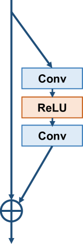
(a) BR block

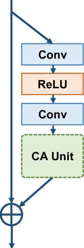
(b) CAR block

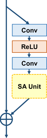
(c) SAR block

Figure 4: Three other blocks for the comparisons with our CSAR block. (a) The base residual (BR) block without any form attention, which corresponds to the $\nth{1}$ and $\nth{5}$ combinations of the first three rows in TABLE I. (b) The channel-wise attention residual (CAR) block corresponding to the $\nth{2}$ and $\nth{6}$ combinations of the first three rows in TABLE I. (c) The spatial attention residual (SAR) block corresponding to the $\nth{3}$ and $\nth{7}$ combinations of the first three rows in TABLE I.

TABLE I:
Ablation Study on Effects of the Channel-wise and Spatial Attention Residual (CSAR) Block and
the Gated Fusion (GF) Node with Long-term Dense Connections.
Average PSNRs for a Scale Factor of $2\times$ on Urban100 Dataset Are Reported.

Components		Different Combinations of Components
In residual blocks	Channel-wise attention (CAR)	×	✓	×	–	×	✓	×	–
	Spatial attention (SAR)	×	×	✓	–	×	×	✓	–
	Combinational attention of CA and SA (CSAR)	×	–	–	✓	×	–	–	✓
Gated fusion (GF) node with long-term dense connections		×	×	×	×	✓	✓	✓	✓
PSNR (dB)		32.38	32.48	32.44	32.54	32.48	32.52	32.50	32.59

III-C Network Architecture

As shown in Fig. 2, we stack multiple FMM modules to build the feature transformation sub-network (FTNet), which is utilized to map the features, generated from the initial feature extraction sub-network (IFENet), to the high informative features for the upscaling sub-network (UpNet). In addition, similar to [12, 13], we also adopt the global residual-feature learning in the FTNet via adding an identity branch from its input to its output (green curve in Fig. 2). Thus, the three sub-networks make up our CSFM network to super-resolve LR image. Let’s denote $\mathbf{X}$ and ${{\mathbf{Y}}_{SR}}$ as the input and output of the CSFM network. And, we adopt a convolutional layer as the IFENet to extract the initial features from LR input image,

$${{\mathbf{F}}_{IFE}}={{S}_{IFENet}}(\mathbf{X}),$$ (12)

where ${{S}_{IFENet}}(\cdot)$ denotes the function of the IFENet, and ${{\mathbf{F}}_{IFE}}$ is a set of extracted features which is then fed into the FTNet and also used for global residual-feature learning.

In the FTNet, the input ${{\mathbf{F}}_{IFE}}$ is firstly sent to a convolutional layer for receptive field expansion and the generated features ${{\mathbf{P}}_{0}}$ are then used as the input to the first FMM module. Supposing $M$ FMM modules and one convolutional layer are stacked to act as the features transformation, the output of the FTNet can be obtained by

$${{\mathbf{F}}_{FT}}={} {{S}_{FTNet}}({{\mathbf{F}}_{IFE}})$$ (13)

$$={} {{f}_{conv}}({{\mathcal{G}}^{(M)}}({{\mathbf{P}}_{0}}))+{{\mathbf{F}}_{IFE}}$$

$$={} {{f}_{conv}}({{\mathcal{G}}_{M}}({{\mathcal{G}}_{M-1}}(\cdots({{\mathcal{G}}_{1}}({{\mathbf{P}}_{0}}))\cdots)))+{{\mathbf{F}}_{IFE}},$$

where ${{S}_{FTNet}}(\cdot)$ represents the FTNet of which the output is ${{\mathbf{F}}_{FT}}$, ${{f}_{conv}}(\cdot)$ is the convolutional operation, ${{\mathcal{G}}_{m}(\cdot)}(m=1,2,\cdots,M)$ denotes the function for the $m\text{-th}$ FMM module as described in Eq. (11).

After acquiring the high informative features ${{\mathbf{F}}_{FT}}$, we exploit the UpNet to upsample them for HR image reconstruction. Specifically, we adopt a sub-pixel convolutional layer [21] followed by a convolutional layer as the UpNet for converting multiple HR sub-images to a single HR image.

$${{\mathbf{Y}}_{SR}}={} {D}(\mathbf{X})$$ (14)

$$={} {{S}_{UpNet}}({{\mathbf{F}}_{FT}})$$

$$={} {{S}_{UpNet}}({{S}_{FTNet}}({{S}_{IFENet}}(\mathbf{X}))),$$

where ${{S}_{UpNet}}(\cdot)$ and ${D}\left(\cdot\right)$ denote the functions of the UpNet and the whole CSFM network respectively.

The CSFM network is optimized via minimizing the difference between the super-resolved image ${{\mathbf{Y}}_{SR}}$ and the corresponding ground-truth image ${\mathbf{Y}}$. As done in previous work [12, 13], we adopt ${{L}_{1}}$ loss function to measure the difference. Given a training dataset $\left\{{{\mathbf{X}}^{k}},{{\mathbf{Y}}^{k}}\right\}_{k=1}^{K}$, where $K$ is the number of training patch pairs and $\left\{{{\mathbf{X}}^{k}},{{\mathbf{Y}}^{k}}\right\}$ are the $k\text{-th}$ LR and HR patch pairs, the objective function for training the CSFM network is formulated as

$${\mathcal{L}}(\Theta)=\frac{1}{K}\sum\limits_{k=1}^{K}{{{\left\|{{\mathbf{Y}}^{k}}-D({{\mathbf{X}}^{k}})\right\|}_{1}}},$$ (15)

where $\Theta$ denotes the parameter set of the CSFM network.

With the stacked FMM modules and the densely connected structure, the proposed CSFM network not only possesses the discriminative learning ability for different types of information but also enables the information that is easier to reconstruct to adopt the shorter forward/backward paths across the network and then pays more attentions to the more important and more difficult information.

IV Experiments and Analysis

In this section, we first provide implementation details, including both model hyper-parameters and training data setting. Then, we study the contributions of different components in the proposed CSFM network by the ablation experiments. Finally, we compare our CSFM model with other state-of-the-art methods on several benchmark datasets.

IV-A Datasets and Metrics

We conduct comparison studies on widely used datasets, Set5 [44], Set14 [45], BSD100 [46], Urban100 [11] and Manga109 [47], which contain 5, 14, 100, 100 and 109 images respectively. The Set5, Set14 and BSD100 contain natural scene images, while the Urban100 consists of urban scene images with many details in different frequency bands and Manga109 is made up of Japanese comic images with many fine structures. We use 800 high-quality training images from DIV2K [48] to train our model. Data augmentation is performed on these training images, which includes random horizontal flipping and random rotation by ${{90}^{\circ}}$.

We use the peak signal-to-noise ratio (PSNR) and the structural similarity (SSIM) [49] index as metrics for evaluation. Higher PSNR and SSIM values indicate better quality. As commonly done in SISR, all the criteria are calculated on the luminance channel of image after pixels near image boundary are removed.

(a) “img015” from Urban100
for $4\times$ upscaling

(b) (a) Ground Truth
PSNR / SSIM

(c) (b) BR
26.55 / 0.7479

(d) (c) CSAR
26.79 / 0.7543

(e) (d) CSAR$+$GF
26.92 / 0.7577

Figure 5: The visual comparisons of super-resolution results by the networks with various combinations of components in TABLE I. The assessments are made for $4\times$ upscaling on the image “img015” from Urban100. (b) is the result produced by the baseline network with BR blocks corresponding to the $\nth{1}$ combination in TABLE I. (c) is generated by the network with proposed CSAR blocks corresponding to the $\nth{4}$ combination in TABLE I. (d) presents the result by the network with both the CSAR blocks and GF nodes corresponding to the last combination in TABLE I. It is obvious that both CSAR blocks for attentive feature-modulation and the GF nodes for long-term information maintenance contribute to generating more faithful result.

IV-B Implementation Details

We apply our model to super-resolve the RGB low-resolution images which are generated by downsampling the corresponding HR images with bicubic kernel to a certain scale. Following [12], we pre-process all images by subtracting the mean RGB values of DIV2K dataset. For training, the LR color patches with a size of $48\times 48$ are randomly cropped from LR images as the inputs of our proposed model and the mini-batch size is set to 16. We train our model with ADAM optimizer [50] by setting ${{\beta}_{1}}=0.9$, ${{\beta}_{2}}=0.999$ and $\varepsilon={{10}^{-8}}$. The initial learning rate is initialized to ${{10}^{-4}}$, which is reduced to half at $\text{3}\times\text{1}{{\text{0}}^{\text{5}}}$ mini-batch updates and then halved at every $\text{2}\times\text{1}{{\text{0}}^{\text{5}}}$ iterations. And, we apply PyTorch [51] on an NVIDIA GTX 1080Ti GPU for model training and testing.

In our CSFM network, all convolutional layers have 64 filters and the kernel sizes of them are $3\times 3$ except the $1\times 1$ convolutional layers in the CA and SA units and those in the GF nodes. Meanwhile, we zero-pad the boundaries of each feature-map to ensure the spatial size of it is the same as the input size after the convolution is operated. In addition, in the CSAR block, the reduction ratio $r$ in the CA unit and the increase ratio $\gamma$ in the SA unit are empirically set to 16 and 2 respectively.

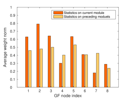
(a) On scale factor $2\times$

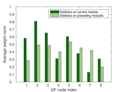
(b) On scale factor $4\times$

Figure 6: The average weight norms of short-term features from the current FMM module and of long-term features from the preceding FMM modules. (a) The statistics are conducted for a scale factor of $2\times$. (b) The statistics are conducted for a scale factor of $4\times$.

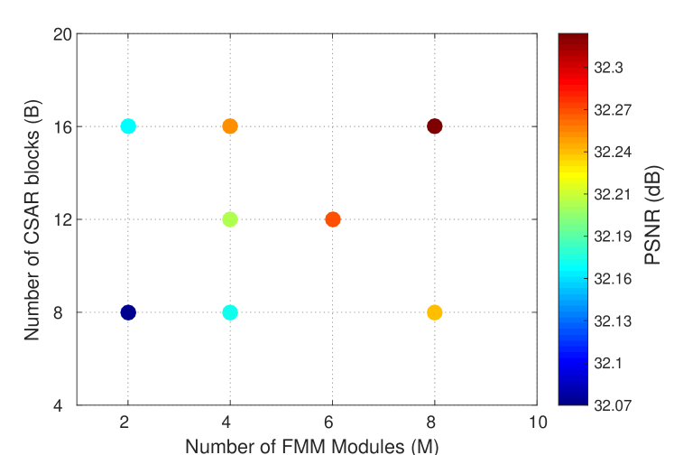
Figure 7: PSNR performance versus the number of FMM modules (M) and the number of CSAR blocks (B) per FMM . The color of the point denotes the PSNR value that corresponds to the color bar on the right. The tests are conducted for a scale factor of $2\times$ on the dataset of BSD100.

IV-C Model Analysis

In this subsection, the contributions of different components and designs in our model are analyzed via the experiments, including the CSAR block, the GF node for information persistence and the performance comparisons of different numbers of the CSAR blocks and the FMM modules. For all experiments, all models utilized for comparisons are trained with $\text{3}\times\text{1}{{\text{0}}^{\text{5}}}$ mini-batch updates for convenience.

IV-C1 The CSAR Block

To validate the effectiveness of the CSAR block, besides the CSAR block, we construct another three blocks for comparison. (I) The base residual (BR) block contains two convolutional layers with one ReLU activation, as shown in Fig. 4(a). Compared with the CSAR block, the BR block removes both the CA unit and SA unit, corresponding to the $\nth{1}$ and $\nth{5}$ combinations of the first three rows in TABLE I. (II) The channel-wise attention residual (CAR) block is constructed by integrating the CA unit to the BR block for adaptively rescaling channel-wise features, which is depicted in Fig. 4(b) and corresponds to the $\nth{2}$ and $\nth{6}$ combinations of the first three rows in TABLE I. (III) The spatial attention residual (SAR) block (the $\nth{3}$ and $\nth{7}$ combinations of the first three rows in TABLE I), as illustrated in Fig. 4(c), is developed by introducing the SA unit into the BR block to modulate pixel-wise features. Specifically, we apply 64 these blocks to the respective networks for experimental comparison, and present SR performances of these networks on Urban100 dataset in TABLE I. Obviously, when the combinational attention of CA and SA is adopted in our CSAR block (the $\nth{4}$ and $\nth{8}$ combinations of the first three rows in TABLE I), the channel-wise attention or the spatial attention needs not be introduced. Therefore, we mark these cases with the symbol of “–” in TABLE I. In addition, Fig. 5 provides the visual comparisons of the network with BR blocks (the $\nth{1}$ combination in TABLE I), the network with CSAR blocks (the $\nth{4}$ combination in TABLE I), and the network with both CSAR blocks and GF nodes (the last combination in TABLE I).

From TABLE I, we can see that when both the CA unit and the SA unit are removed in the BR block, the PSNR values are relatively low, especially when the GF nodes are not used for long-term information preservation. And, by integrating the CA unit or the SA unit into the BR blocks, the SR performances can be moderately improved. Moreover, when our proposed CSAR blocks with the combinational attentions are utilized, the performance can be further boosted. In both cases of without and with the GF nodes, the network with the CSAR blocks outperforms those with the BR blocks by the PSNR gains of 0.16dB and 0.11dB respectively. Furthermore, in Fig. 5, it is seen that the network only with BR blocks (Fig. 5(b)) generates some blurry and false fence lines while the network with proposed CSAR blocks (Fig. 5(c)) accurately reconstructs the fence rows and presents better result via combining the channel-wise and spatial attentions. The above observations demonstrate the superiority of our CSAR block over other blocks without attention or with only one type of attention (i.e. the BR block, CAR block and SAR block), and also manifest that integrating channel-wise and spatial attentions in residual blocks to modulate multi-level features can benefit image SR.

TABLE II:
Quantitative Evaluations of State-of-the-art SR Methods.
The Average PSNRs/SSIMs for Scale Factors of $2\times$, $3\times$ and $4\times$ Are Reported.
Fontbold Indicates the Best Performance and Underline Indicates the Second-best Performance.

Scale	Method	Set5		Set14		BSD100		Urban100		Manga109
		PSNR	SSIM	PSNR	SSIM	PSNR	SSIM	PSNR	SSIM	PSNR	SSIM
$2\times$	Bicubic	33.68	0.9304	30.24	0.8691	29.56	0.8435	26.88	0.8405	30.81	0.9348
	SRCNN [14]	36.66	0.9542	32.45	0.9067	31.36	0.8879	29.51	0.8946	35.70	0.9677
	FSRCNN [20]	36.98	0.9556	32.62	0.9087	31.50	0.8904	29.85	0.9009	36.56	0.9703
	VDSR [15]	37.53	0.9587	33.05	0.9127	31.90	0.8960	30.77	0.9141	37.41	0.9747
	LapSRN [27]	37.52	0.9591	32.99	0.9124	31.80	0.8949	30.41	0.9101	37.27	0.9740
	DRRN [16]	37.74	0.9591	33.23	0.9136	32.05	0.8973	31.23	0.9188	37.88	0.9750
	MemNet [19]	37.78	0.9597	33.28	0.9142	32.08	0.8978	31.31	0.9195	38.02	0.9755
	IDN [31]	37.83	0.9600	33.30	0.9148	32.08	0.8985	31.27	0.9196	38.02	0.9749
	EDSR [12]	38.11	0.9601	33.92	0.9195	32.32	0.9013	32.93	0.9351	39.19	0.9782
	SRMDNF [52]	37.79	0.9601	33.32	0.9154	32.05	0.8984	31.33	0.9204	38.07	0.9761
	D-DBPN [29]	38.13	0.9609	33.83	0.9201	32.28	0.9009	32.54	0.9324	38.89	0.9775
	RDN [13]	38.24	0.9614	34.01	0.9212	32.34	0.9017	32.89	0.9353	39.18	0.9780
	CSFM (ours)	38.26	0.9615	34.07	0.9213	32.37	0.9021	33.12	0.9366	39.40	0.9785
$3\times$	Bicubic	30.40	0.8686	27.54	0.7741	27.21	0.7389	24.46	0.7349	26.95	0.8565
	SRCNN [14]	32.75	0.9090	29.29	0.8215	28.41	0.7863	26.24	0.7991	30.56	0.9125
	FSRCNN [20]	33.16	0.9140	29.42	0.8242	28.52	0.7893	26.41	0.8064	31.12	0.9196
	VDSR [15]	33.66	0.9213	29.78	0.8318	28.83	0.7976	27.14	0.8279	32.13	0.9348
	LapSRN [27]	33.82	0.9227	29.79	0.8320	28.82	0.7973	27.07	0.8271	32.21	0.9344
	DRRN [16]	34.03	0.9244	29.96	0.8349	28.95	0.8004	27.53	0.8378	32.74	0.9388
	MemNet [19]	34.09	0.9248	30.00	0.8350	28.96	0.8001	27.56	0.8376	32.79	0.9391
	IDN [31]	34.11	0.9253	29.99	0.8354	28.95	0.8013	27.42	0.8359	32.69	0.9378
	EDSR [12]	34.65	0.9282	30.52	0.8462	29.25	0.8093	28.80	0.8653	34.20	0.9486
	SRMDNF [52]	34.12	0.9254	30.04	0.8371	28.97	0.8025	27.57	0.8398	33.00	0.9403
	RDN [13]	34.71	0.9296	30.57	0.8468	29.26	0.8093	28.80	0.8653	34.13	0.9484
	CSFM (ours)	34.76	0.9301	30.63	0.8477	29.30	0.8105	28.98	0.8681	34.52	0.9502
$4\times$	Bicubic	28.43	0.8109	26.00	0.7023	25.96	0.6678	23.14	0.6574	24.89	0.7875
	SRCNN [14]	30.48	0.8628	27.50	0.7513	26.90	0.7103	24.52	0.7226	27.63	0.8553
	FSRCNN [20]	30.70	0.8657	27.59	0.7535	26.96	0.7128	24.60	0.7258	27.85	0.8557
	VDSR [15]	31.35	0.8838	28.02	0.7678	27.29	0.7252	25.18	0.7525	28.87	0.8865
	LapSRN [27]	31.54	0.8866	28.09	0.7694	27.32	0.7264	25.21	0.7553	29.09	0.8893
	DRRN [16]	31.68	0.8888	28.21	0.7720	27.38	0.7284	25.44	0.7638	29.45	0.8946
	MemNet [19]	31.74	0.8893	28.26	0.7723	27.40	0.7281	25.50	0.7630	29.64	0.8971
	IDN [31]	31.82	0.8903	28.25	0.7730	27.41	0.7297	25.41	0.7632	29.41	0.8936
	EDSR [12]	32.46	0.8968	28.80	0.7876	27.71	0.7420	26.64	0.8033	31.03	0.9158
	SRMDNF [52]	31.96	0.8925	28.35	0.7772	27.49	0.7337	25.68	0.7731	30.09	0.9024
	D-DBPN [29]	32.42	0.8977	28.76	0.7862	27.68	0.7393	26.38	0.7946	30.91	0.9137
	RDN [13]	32.47	0.8990	28.81	0.7871	27.72	0.7419	26.61	0.8028	31.00	0.9151
	CSFM (ours)	32.61	0.9000	28.87	0.7886	27.76	0.7432	26.78	0.8065	31.32	0.9183

IV-C2 The GF Node with Long-term Dense Connections

As illustrated in Fig. 2(b), the GF node is added at the end of the FMM module for contributing to persistent memory maintenance and different information fusion. To investigate the contributions of the GF node, we conduct the ablation tests and present the study on the effect of the GF node in TABLE I and Fig. 5. In TABLE I, the first four columns list the results produced by the networks without GF nodes where 64 blocks are cascaded for feature transformation, while the last four columns show the performances of the networks with GF nodes in which 16 blocks and one GF node constitute a module and 4 modules are stacked with densely connected structure (similar to the architecture of the CSFM network). Through the comparisons between the results in the first four columns and those in the last four columns, we find that the networks with GF nodes would perform better than those without GF nodes. Specifically, when the CSAR blocks with combinational attentions are utilized, the network with GF nodes can achieve an improvement of 0.21dB in terms of PSNR compared with the baseline network with only BR blocks. Besides, from Fig. 5, we can observe that by introducing information maintenance mechanism, the network with GF nodes generates finer and clearer fence rows compared with those without GF nodes. These comparisons manifest that applying the GF nodes makes long-term information preservation easy and then more important information can be effectively exploited for image SR.

To further analyze the contributions of different kinds of information fed into the GF nodes and illustrate how the GF nodes control the output information, and inspired by [19], we make statistics on the norms of the weights from all filters in the GF nodes. For each feature-map input to the GF node, we calculate the weight norm in the corresponding filter as follows

$$q_{n}^{m}=\sqrt{\sum\limits_{i=1}^{64}{{{\left(\mathbf{W}_{GF}^{m}\left[i,n,1,1\right]\right)}^{2}}}}$$ (16)

where $q_{n}^{m}\left(n=1,2,\cdots,{{N}_{m}}\right)$ represents the weight norm of the $n\text{-th}$ feature-map fed into the $m\text{-th}$ GF node (receiving ${{N}_{m}}$ feature-maps as input), and $\mathbf{W}_{GF}^{m}$ with size of $64\times{{N}_{m}}\times 1\times 1$ denotes the weight set of the filter in the GF node. The larger norm indicates that the feature-map provides more information to the GF node for fusion, and vice versa. For the sake of comparison, we average the weight norms of long-term feature-maps from the preceding FMM modules and of short-term feature-maps from the current FMM module respectively. Similar to [19], we normalize the weight norms to the range of 0 to 1 for better visualization. Fig. 6 presents the average norms of two types of feature-maps (long-term feature-maps and short-term feature-maps) in eight GF nodes of eight FMM modules for two scale factors of $2\times$ and $4\times$. One can see that the long-term information from the preceding modules makes non-negligible contribution especially in late modules whatever the upscaling factor is, which indicates that the long-term information plays an important role in super-resolving LR image. Therefore, the GF nodes being added for information persistence is beneficial for improving SR performance.

Ground Truth PSNR / SSIM IDN [31] 18.27 / 0.6176 Bicubic 16.58 / 0.4374 EDSR [12] 19.14 / 0.6779 SRCNN [14] 17.56 / 0.5413 SRMDNF [52] 18.57 / 0.6308 VDSR [15] 18.14 / 0.6011 D-DBPN [29] 18.92 / 0.6602 LapSRN [27] 18.20 / 0.6078 RDN [13] 19.18 / 0.6770 MemNet [19] 18.59 / 0.6397 CSFM (Ours) 20.17 / 0.7157

Figure 8: Visual evaluation for a scale factor of $4\times$ on the image “img092” from Urban100. Our CSFM network accurately reconstructs clearer stripes while other methods produce blurry results with wrong directions.

Ground Truth PSNR / SSIM IDN [31] 22.22 / 0.6974 Bicubic 21.57 / 0.6287 EDSR [12] 23.94 / 0.7746 FSRCNN [20] 22.00 / 0.6769 SRMDNF [52] 22.46 / 0.7109 VDSR [15] 22.15 / 0.6920 D-DBPN [29] 23.19 / 0.7439 LapSRN [27] 22.01 / 0.6917 RDN [13] 24.07 / 0.7799 DRRN [16] 21.93 / 0.6897 CSFM (Ours) 24.31 / 0.7858

Figure 9: Visual evaluation for a scale factor of $4\times$ on the image “img076” from Urban100. Other methods fail to recover the texture region on the face and give very tangle results. By contrast, our CSFM model can reconstruct the details which are subjectively closer to the ground truth.

Ground Truth PSNR / SSIM IDN [31] 33.13 / 0.9428 Bicubic 27.52 / 0.8578 EDSR [12] 34.60 / 0.9559 SRCNN [14] 30.84 / 0.9123 SRMDNF [52] 33.52 / 0.9476 VDSR [15] 32.26 / 0.9387 D-DBPN [29] 34.39 / 0.9545 LapSRN [27] 32.57 / 0.9396 RDN [13] 34.41 / 0.9558 MemNet [19] 32.99 / 0.9445 CSFM (Ours) 35.01 / 0.9586

Figure 10: Visual evaluation for a scale factor of $4\times$ on the image “PsychoStaff” from Manga109. Only our CSFM network can recover more recognizable characters which are too vague to be recognized in other results.

Ground Truth PSNR / SSIM IDN [31] 26.66 / 0.8600 Bicubic 22.86 / 0.7403 EDSR [12] 28.97 / 0.9076 FSRCNN [20] 24.84 / 0.8034 SRMDNF [52] 27.19 / 0.8744 VDSR [15] 25.92 / 0.8428 D-DBPN [29] 28.22 / 0.8937 LapSRN [27] 25.98 / 0.8455 RDN [13] 28.94 / 0.9072 DRRN [16] 26.57 / 0.8608 CSFM (Ours) 29.45 / 0.9138

Figure 11: Visual evaluation for a scale factor of $4\times$ on the image “img087” from Urban100. Only our CSFM model correctly reconstructs the color lines on the balcony while other methods generate fuzzier lines with wrong colors and structures.

Ground Truth PSNR / SSIM IDN [31] 23.01 / 0.6591 Bicubic 22.16 / 0.5552 EDSR [12] 24.22 / 0.7351 SRCNN [14] 22.73 / 0.6133 SRMDNF [52] 23.41 / 0.6753 VDSR [15] 23.09 / 0.6415 D-DBPN [29] 23.99 / 0.7232 LapSRN [27] 23.15 / 0.6520 RDN [13] 24.29 / 0.7445 MemNet [19] 23.22 / 0.6676 CSFM (Ours) 24.38 / 0.7544

Figure 12: Visual evaluation for a scale factor of $4\times$ on the image “img074” from Urban100. The reconstructed grids produced by our CSFM network are more faithful and sharper than those by other methods.

Ground Truth PSNR / SSIM IDN [31] 27.36 / 0.8879 Bicubic 24.66 / 0.7861 EDSR [12] 29.05 / 0.9243 FSRCNN [20] 26.33 / 0.8440 SRMDNF [52] 27.51 / 0.8897 VDSR [15] 27.00 / 0.8744 D-DBPN [29] 28.27 / 0.9079 LapSRN [27] 26.92 / 0.8752 RDN [13] 28.24 / 0.9121 DRRN [16] 27.25 / 0.8826 CSFM (Ours) 29.88 / 0.9379

Figure 13: Visual evaluation for a scale factor of $4\times$ on the image “YumeiroCooking” from Manga109. Our CSFM model can generate finer textures on the sleeves in contrast with other methods which produce the results with severe distortions and heavy blurring artifacts.

IV-C3 The Number of FMM Modules and the Number of CSAR Blocks in each FMM Module

The capacity of the CSFM network is mainly determined by the number of the FMM modules and the number of the CSAR blocks in each FMM module. In this subsection, we test the effects of two parameters on image SR. For simplicity, we denote the number of the FMM modules as $M$ and the number of the CSAR blocks as $B$. The network with $m$ modules and $b$ blocks per module is represented as $MmBb$ for short.

Fig. 7 shows the results of the PSNR performance (illustrated by different colors according to the color bar on the right) versus two parameters ($M$ and $B$) on the dataset of BSD100 for a scale factor of $2\times$. We can see that the better performances can be achieved by increasing $M$ or $B$. Since the larger $M$ and $B$ results in a deeper network, the comparisons in Fig. 7 suggest that the deeper model is still advantageous. On the other hand, compared with $M4B8$ (achieving 32.212dB on PSNR), $M2B16$ (obtaining 32.208dB on PSNR) with the same total number of CSAR blocks achieves comparable performance although it has fewer GF nodes for long-term skip connections, and the similar observation can be obtained in the comparison between $M4B16$ and $M8B8$. These results indicate that properly utilizing the limited number of skip connections does not lose accuracy but reduces the redundancy and computational cost. To effectively exploit long-term skip connections for information persistence as well as control the computational cost, we adopt $M=8$ and $B=16$ as our CSFM model for the next comparison experiments.

IV-D Comparisons with the State-of-the-arts

To illustrate the effectiveness of the proposed CSFM network, several state-of-the-art SISR methods, including SRCNN [14], FSRCNN [20], VDSR [15], LapSRN [27], DRRN [16], MemNet [19], IDN [31], EDSR [12], SRMDNF [52], D-DBPN [29] and RDN [13], are compared in terms of quantitative evaluation, visual quality and number of parameters. Since some of existing networks, such as SRCNN, FSRCNN, VDSR, DRRN, MemNet, EDSR and IDN, did not perform SR on Manga109 dataset, we generate the corresponding results by applying their public trained models to Manga109 dataset for evaluation. In addition, we rebuild the VDSR network in PyTorch with the same network parameters for training and testing as its trained model is not provided.

The quantitative evaluations in the five benchmark datasets for three scale factors ($2\times$, $3\times$, $4\times$) are summarized in TABLE II. When compared with MemNet and RDN, both of which introduce persistence memory mechanism via extremely dense skip connections, our CSFM network achieves the highest performance but with fewer skip connections. This indicates that our FMM module with long-term skip connections not only advances the memory block in MemNet [19] and the residual dense block in RDN [13] but also reduces the redundancy in the structure of extremely dense connections. Meanwhile, our CSFM model significantly outperforms the remaining methods on all datasets for all upscaling factors, in terms of PSNR and SSIM. Especially, on the challenging dataset Urban100, the proposed CSFM network advances the state-of-the-art (achieved by EDSR or RDN) with the improvement margins of 0.19dB, 0.18dB and 0.14dB on scale factors of $2\times$, $3\times$ and $4\times$ respectively. In addition, more significant improvements earned by the CSFM network are shown on Manga109 dataset, where the proposed CSFM model outperforms EDSR (with highest performance among the prior methods) by the PSNR gains of 0.21dB, 0.32dB and 0.29dB for the $2\times$, $3\times$ and $4\times$ enlargement respectively. These results validate the superiority of the proposed method especially on super-resolving the images with fine structures such as those in Urban100 and Manga109 datasets.

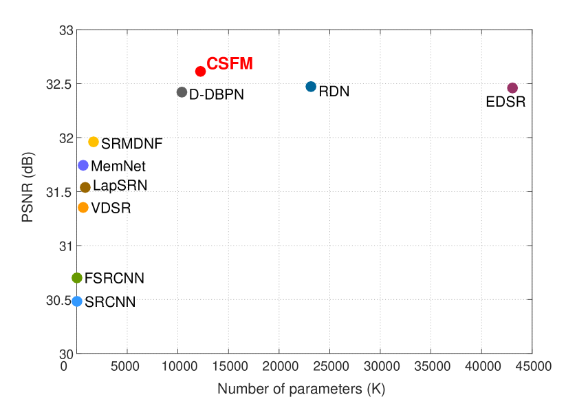
Figure 14: PSNR performance versus number of parameters. The results are evaluated on Set5 dataset for a scale factor of $4\times$. Our CSFM network has a better tradeoff between performance and model size.

The visual comparisons of different methods are shown in Fig. 8 – Fig. 13. Thanks to the proposed FMM modules for adaptive multi-level feature-modulation and long-term memory preservation, our proposed CSFM network accurately and clearly reconstructs the stripe patterns, the grid structures, the texture regions and the characters. It is observed that the severe distortions and the noticeable artifacts are contained in the results generated by the prior methods, such as the marked strips on the wall in Fig. 8, the color lines on the balcony in Fig. 11 and the grids on the building in Fig. 12. In contrast, our method avoids the distortions, suppresses the artifacts and generates more faithful results. Besides, in Fig. 9, Fig. 13 and Fig. 10, only our method is able to recover more accurate textures and more recognizable characters, while other methods suffer from much information loss and heavy blurring artifacts. The above visual comparisons demonstrate the powerful representational ability of our CSFM network as well.

We also compare the tradeoff between the performance and the number of network parameters from our CSFM network and existing networks. Fig. 14 shows the PSNR performances of several models versus the number of parameters, where the results are evaluated with Set5 dataset for $4\times$ upscaling factor. We can see that our CSFM network significantly outperforms the relatively small models. Furthermore, compared with EDSR and RDN, our CSFM network achieves higher PSNR but with 72% and 47% fewer parameters respectively. These comparisons indicate that our model has a better tradeoff between performance and model size.

V Conclusion

In this paper, we propose a channel-wise and spatial feature modulation (CSFM) network for modeling the process of single image super-resolution, where stacked feature-modulation memory (FMM) modules with the densely connected structure effectively improve its discriminative learning ability and make it concentrate on the worthwhile information. The FMM module consists of a chain of cascaded channel-wise and spatial attention residual (CSAR) blocks and a gated fusion (GF) node. The CSAR block is constructed by incorporating the channel-wise attention and spatial attention into the residual block and utilized to modulate the residual features in a global-and-local way. Further, when a sequence of CSAR blocks are cascaded in the FMM module, two types of attention can be jointly applied to multi-level features and then more informative features can be captured. Meanwhile, The GF node, designed via introducing the gating mechanism and for establishing long-term skip connections among the FMM modules, can help to maintain long-term information and enhance information flow. Comprehensive evaluations on benchmark datasets demonstrate better performance of our CSFM network in terms of quantitative and qualitative measurements.

References

- [1] W. T. Freeman, E. C. Pasztor, and O. T. Carmichael, “Learning low-level vision,” Int. J. Comput. Vis., vol. 40, no. 1, pp. 25–47, Oct. 2000.
- [2] G. Polatkan, M. Zhou, L. Carin, and D. Blei, “A Bayesian non-parametric approach to image super-resolution,” IEEE Trans. Pattern Anal. Mach. Intell., vol. 37, no. 2, pp. 346–358, Feb. 2015.
- [3] H. Chang, D.-Y. Yeung, and Y. Xiong, “Super-resolution through neighbor embedding,” in Proc. IEEE Conf. Comput. Vis. Pattern Recognit. (CVPR), Jun./Jul. 2004, pp. 275–282.
- [4] J. Jiang, R. Hu, Z. Wang, Z. Han, and J. Ma, “Facial image hallucination through coupled-layer neighbor embedding,” IEEE Trans. Circuits Syst. Video Technol., vol. 26, no. 9, pp. 1674–1684, Sep. 2016.
- [5] J. Yang, J. Wright, T. S. Huang, and Y. Ma, “Image super-resolution via sparse representation,” IEEE Trans. Image Process., vol. 19, no. 11, pp. 2861–2873, Nov. 2010.
- [6] L. He, H. Qi, and R. Zaretzki, “Beta process joint dictionary learning for coupled feature spaces with application to single image super-resolution,” in Proc. IEEE Conf. Comput. Vis. Pattern Recognit. (CVPR), Jun. 2013, pp. 345–352.
- [7] R. Timofte, V. D. Smet, and L. V. Gool, “A+: adjusted anchored neighborhood regression for fast super-resolution,” in Proc. 12th Asian Conf. Comput. Vis. (ACCV), Nov. 2014, pp. 111–126.
- [8] Y. Hu, N. Wang, D. Tao, X. Gao, and X. Li, “SERF: a simple, effective, robust, and fast image super-resolver from cascaded linear regression,” IEEE Trans. Image Process., vol. 25, no. 9, pp. 4091–4102, Sep. 2016.
- [9] J. Huang and W. Siu, “Learning hierarchical decision trees for single-image super-resolution,” IEEE Trans. Circuits Syst. Video Technol., vol. 27, no. 5, pp. 937–950, May. 2017.
- [10] S. Schulter, C. Leistner, and H. Bischof, “Fast and accurate image upscaling with super-resolution forests,” in Proc. IEEE Conf. Comput. Vis. Pattern Recognit. (CVPR), Jun. 2015, pp. 3791–3799.
- [11] J.-B. Huang, A. Singh, and N. Ahuja, “Single image super-resolution from transformed self-exemplars,” in IEEE Conf. Comput. Vis. Pattern Recognit. (CVPR), Jun. 2015, pp. 5197–5206.
- [12] B. Lim, S. Son, H. Kim, S. Nah, and K. M. Lee, “Enhanced deep residual networks for single image super-resolution,” in Proc. IEEE Conf. Comput. Vis. Pattern Recognit. Workshops (CVPRW), Jul. 2017, pp. 136–144.
- [13] Y. Zhang, Y. Tian, Y. Kong, B. Zhong, and Y. Fu, “Residual dense network for image super-resolution,” in Proc. IEEE Conf. Comput. Vis. Pattern Recognit. (CVPR), Jun. 2018, pp. 2472–2481.
- [14] C. Dong, C. C. Loy, K. He, and X. Tang, “Image super-resolution using deep convolutional networks,” IEEE Trans. Pattern Anal. Mach. Intell., vol. 38, no. 2, pp. 295–307, Feb. 2016.
- [15] J. Kim, J. K. Lee, and K. M. Lee, “Accurate image super-resolution using very deep convolutional networks,” in Proc. IEEE Conf. Comput. Vis. Pattern Recognit. (CVPR), Jun. 2016, pp. 1646–1654.
- [16] Y. Tai, J. Yang, and X. Liu, “Image super-resolution via deep recursive residual network,” in Proc. IEEE Conf. Comput. Vis. Pattern Recognit. (CVPR), Jul. 2017, pp. 3147–3155.
- [17] J. Kim, and J. K. Lee, and K. M. Lee, “Deeply-recursive convolutional network for image super-resolution,” in Proc. IEEE Conf. Comput. Vis. Pattern Recognit. (CVPR), Jun. 2016, pp. 1637–1645.
- [18] X.-J. Mao, C. Shen, and Y.-B. Yang, “Image restoration using very deep convolutional encoder-decoder networks with symmetric skip connections,” in Proc. Adv. Neural Inf. Process. Syst. (NIPS), Dec. 2016, pp. 2802–2810.
- [19] Y. Tai, J. Yang, X. Liu, and C. Xu, “MemNet: a persistent memory network for image restoration,” in Proc. IEEE Int. Conf. Comput. Vis. (ICCV), Oct. 2017, pp. 4549–4557.
- [20] C. Dong, C. C. Loy, and X. Tang, “Accelerating the super-resolution convolutional neural network,” in Proc. Eur. Conf. Comput. Vis. (ECCV), Oct. 2016, pp. 391–407.
- [21] W. Shi, J. Caballero, F. Huszar, J. Totz, A. P. Aitken, R. Bishop, D. Rueckert, and Z. Wang, “Real-time single image and video super-resolution using an efficient sub-pixel convolutional neural network,” in Proc. IEEE Conf. Comput. Vis. Pattern Recognit. (CVPR), Jun. 2016, pp. 1874–1883.
- [22] C. Ledig, L. Theis, F. Huszar, J. Caballero, A. P. Aitken, A. Tejani, J. Totz, Z. Wang, and W. Shi, “Photo-realistic single image super-resolution using a generative adversarial network,” in Proc. IEEE Conf. Comput. Vis. Pattern Recognit. (CVPR), Jul. 2017, pp. 105–114.
- [23] K. He, X. Zhang, S. Ren, and J. Sun, “Deep residual learning for image recognition,” in Proc. IEEE Conf. Comput. Vis. Pattern Recognit. (CVPR), Jun. 2016, pp. 770–778.
- [24] G. Huang, Z. Liu, K. Q. Weinberger, and L. van der Maaten, “Densely connected convolutional networks,” in Proc. IEEE Conf. Comput. Vis. Pattern Recognit. (CVPR), Jul. 2017, pp. 4700–4708.
- [25] T. Tong, G. Li, X. Liu, and Q. Gao, “Image super-resolution using dense skip connections,” in Proc. IEEE Int. Conf. Comput. Vis. (ICCV), Oct. 2017, pp. 4799–4807.
- [26] Y. Wang, F. Perazzi, B. McWilliams, A. Sorkine-Hornung, O. Sorkine-Hornung, and C. Schroers, “A fully progressive approach to single-image super-resolution,” in Proc. IEEE Conf. Comput. Vis. Pattern Recognit. Workshops (CVPRW), Jun. 2018, pp. 977–986.
- [27] W.-S. Lai, J.-B. Huang, N. Ahuja, and M.-H. Yang, “Deep Laplacian pyramid networks for fast and accurate super-resolution,” in Proc. IEEE Conf. Comput. Vis. Pattern Recognit. (CVPR), Jul. 2017, pp. 624–632.
- [28] Z. He, S. Tang, J. Yang., Y. Cao, M. Y. Yang, and Y. Cao, “Cascaded deep networks with multiple receptive fields for infrared image super-resolution,” IEEE Trans. Circuits Syst. Video Technol., 2018.
- [29] M. Haris, G. Shakhnarovich, and N. Ukita, “Deep back-projection networks for super-resolution,” in Proc. IEEE Conf. Comput. Vis. Pattern Recognit. (CVPR), Jun. 2018, pp. 1664–1673.
- [30] S. Zagoruyko and N. Komodakis, “Image super-resolution via dual-state recurrent networks,” arXiv: 1805.02704, May. 2018.
- [31] Z. Hui, X. Wang, and X. Gao, “Fast and accurate single image super-resolution via information distillation network,” in Proc. IEEE Conf. Comput. Vis. Pattern Recognit. (CVPR), Jun. 2018, pp. 723–731.
- [32] J.-H. Kim and J.-S. Lee, “Deep residual network with enhanced upscaling module for super-resolution,” in Proc. IEEE Conf. Comput. Vis. Pattern Recognit. Workshops (CVPRW), Jun. 2018, pp. 913–921.
- [33] E. Mansimov, E. Parisotto, J. L. Ba, and R. Salakhutdinov, “Generating images from captions with attention,” in Int. Conf. Learn. Rep. (ICLR), May. 2016, pp. 1–4.
- [34] K. Xu, J. Ba, R. Kiros, K. Cho, A. Courville, R. Salakhutdinov, R. S. Zemel, and Y. Bengio, “Show, attend and tell: Neural image caption generation with visual attention,” in Int. Conf. Mach. Learn. (ICML), Jul. 2015, pp. 2048–2057.
- [35] L. Chen, H. Zhang, J. Xiao, L. Nie, J. Shao, W. Liu, and T.-S. Chua, “Sca-cnn: Spatial and channel-wise attention in convolutional networks for image captioning,” in Proc. IEEE Conf. Comput. Vis. Pattern Recognit. (CVPR), Jul. 2017, pp. 5659–5667.
- [36] J. Hu, L. Shen, and G. Sun, “Squeeze-and-excitation networks,” in Proc. IEEE Conf. Comput. Vis. Pattern Recognit. (CVPR), Jun. 2018, pp. 7132–7141.
- [37] F. Wang, M. Jiang, C. Qian, S. Yang, C. Li, H. Zhang, X. Wang, and X. Tang, “Residual attention network for image classification,” in Proc. IEEE Conf. Comput. Vis. Pattern Recognit. (CVPR), Jul. 2017, pp. 3156–3164.
- [38] Y. Zhang, K. Li, K. Li, L. Wang, B. Zhong, and Y. Fu, “Image super-resolution using very deep residual channel attention networks,” in Proc. Eur. Conf. Comput. Vis. (ECCV), Sept. 2018, pp. 1–16.
- [39] X. Wang, K. Yu, C. Dong, and C. C. Loy, “Recovering realistic texture in image super-resolution by deep spatial feature transform,” in Proc. IEEE Conf. Comput. Vis. Pattern Recognit. (CVPR), Jun. 2018, pp. 606–615.
- [40] H. Xu and K. Saenko, “Ask, attend and answer: Exploring question guided spatial attention for visual question answering,” in Proc. Eur. Conf. Comput. Vis. (ECCV), Oct. 2016, pp. 451–466.
- [41] Y. Chen, J. Li, H. Xiao, X. Jin, S. Yan, and J. Feng, “Dual path networks,” in Proc. Adv. Neural Inf. Process. Syst. (NIPS), Dec. 2017, pp. 1–9.
- [42] V. Nair and G. Hinton, “Rectified linear units improve restricted boltzmann machines,” in Int. Conf. Mach. Learn. (ICML), Jun. 2010, pp. 807–814.
- [43] L. Itti and C. Koch, “Computational modelling of visual attention,” Nat. Rev. Neurosci., vol. 2, no. 3, pp. 194–203, Mar. 2001.
- [44] M. Bevilacqua, A. Roumy, C. Guillemot, and M.-L. A. Morel, “Low-complexity single-image super-resolution based on nonnegative neighbor embedding,” in Proc. 23rd British Mach. Vis. Conf. (BMVC), Sep. 2012, pp. 135.1–135.10.
- [45] R. Zeyde, M. Elad, and M. Protter, “On single image scale-up using sparse-representations,” in Proc. 7th Int. Conf. Curves Surfaces, Jun. 2010, pp. 711–730.
- [46] P. Arbeláez, M. Maire, C. Fowlkes, and J. Malik, “Contour detection and hierarchical image segmentation,” IEEE Trans. Pattern Anal. Mach. Intell., vol. 33, no. 5, pp. 898–916, May. 2011.
- [47] Y. Matsui, K. Ito, Y. Aramaki, A. Fujimoto, T. Ogawa, T. Yamasaki, and K. Aizawa, “Sketch-based manga retrieval using manga109 dataset,” Multimedia Tools Appl., vol. 76, no. 20, pp. 21 811–21 838, Oct. 2017.
- [48] R. Timofte, E. Agustsson, L. V. Gool, M.-H. Yang, L. Zhang, B. Lim, and et al., “NTIRE 2017 challenge on single image super-resolution: methods and results,” in Proc. IEEE Conf. Comput. Vis. Pattern Recognit. Workshops (CVPRW), Jul. 2017, pp. 1110–1121.
- [49] Z. Wang, A. C. Bovik, H. R. Sheikh, and E. P. Simoncelli, “Image quality assessment: from error visibility to structural similarity,” IEEE Trans. Image Process., vol. 13, no. 4, pp. 600–612, Apr. 2004.
- [50] D. P. Kingma and J. Ba, “Adam: A method for stochastic optimization,” in Int. Conf. Learn. Rep. (ICLR), May. 2015, pp. 1–13.
- [51] A. Paszke, S. Gross, S. Chintala, G. Chanan, E. Yang, Z. DeVito, Z. Lin, A. Desmaison, L. Antiga, and A. Lerer, “Automatic differentiation in PyTorch,” in Proc. Adv. Neural Inf. Process. Syst. Workshop Autodiff, Dec. 2015, pp. 1–4.
- [52] K. Zhang, W. Zuo, and L. Zhang, “Learning a single convolutional super-resolution network for multiple degradations,” in Proc. IEEE Conf. Comput. Vis. Pattern Recognit. (CVPR), Jun. 2018, pp. 3262–3271.