Is there a Floquet Lindbladian?

Abstract

The stroboscopic evolution of a time-periodically driven isolated quantum system can always be described by an effective time-independent Hamiltonian. Whether this concept can be generalized to open Floquet systems, described by a Markovian master equation with time-periodic Lindbladian generator, remains an open question. By using a two level system as a model, we explicitly show the existence of two well-defined parameter regions. In one region the stroboscopic evolution can be described by a Markovian master equation with a time-independent Floquet Lindbladian. In the other it cannot; but here the one-cycle evolution operator can be reproduced with an effective non-Markovian master equation that is homogeneous but non-local in time. Interestingly, we find that the boundary between the phases depends on when the evolution is stroboscopically monitored. This reveals the non-trivial role played by the micromotion in the dynamics of open Floquet systems.

When the coherent evolution of an isolated quantum Floquet system, described by the time-periodic Hamiltonian $H(t)=H(t+T)$, is monitored stroboscopically in steps of the driving period $T$, this dynamics is described by repeatedly applying the one-cycle time-evolution operator $U(T)=\mathcal{T}\exp\big{[}-\frac{i}{\hbar}\int_{0}^{T}\!\mathrm{d}t^{\prime}H(t^{\prime})\big{]}$ (with time ordering $\mathcal{T}$) Shirley (1965); Sambe (1973). It can always be expressed in terms of an effective time-independent Hamiltonian $H_{F}$, called Floquet Hamiltonian, $U(T)\equiv\exp(-iH_{F}T/\hbar)$. While the Floquet Hamiltonian is not unique due to the multi-branch structure of the operator logarithm $\log U(T)$, the unitarity of $U(T)$ implies that $H_{F}$ is Hermitian (like a proper Hamiltonian) for every branch. The concept of the Floquet Hamiltonian suggests a form of quantum engineering, where a suitable time-periodic driving protocol is designed in order to effectively realize a system described by a Floquet Hamiltonian with desired novel properties. This type of Floquet engineering was successfully employed with ultracold atoms Eckardt (2017), e.g. to realize artificial magnetic fields and topological band structures for charge neutral particles Aidelsburger et al. (2011); Rechtsman et al. (2013); Struck et al. (2013); Jotzu et al. (2014); Aidelsburger et al. (2015); Fläschner et al. (2016).

However, systems like atomic quantum gases, which are very well isolated from their environment, should rather be viewed as an exception. Many quantum systems that are currently studied in the laboratory and used for technological applications are based on electronic or photonic degrees of freedom that usually couple to their environment. It is, therefore, desirable to extend the concept of Floquet engineering also to open systems. In this context, a number of papers investigating properties of the non-equilibrium steady states approached by periodically modulated dissipative systems in the long-time limit have been published Breuer et al. (2000); Alicki et al. (2006); Ketzmerick and Wustmann (2010); Vorberg et al. (2013); Shirai et al. (2015); Seetharam et al. (2015, 2015); Dehghani et al. (2015); Iadecola et al. (2015); Vorberg et al. (2015); Shirai et al. (2016); Letscher et al. (2017); Schnell et al. (2018); Chong et al. (2018); Qin et al. (2018); Higashikawa et al. (2018). In this paper, in turn, we are interested in the (transient) dynamics of open Floquet systems and address the question as to whether it is possible to describe their stroboscopic evolution with time-independent generators that generalize the concept of the Floquet Hamiltonian to open systems.

We consider a time-dependent Markovian master equation Breuer et al. (2009)

$$\dot{\rho}=\mathcal{L}(t)\rho=\frac{1}{i\hbar}[H(t),\rho]+\mathcal{D}(t)\rho,$$ (1)

for the system’s density operator $\rho$ (with Hilbert space dimension $N$), described by a time-periodic generator $\mathcal{L}(t)=\mathcal{L}(t+T)$. It is characterized by a Hermitian time-periodic Hamiltonian $H(t)$ and a dissipator

$$\mathcal{D}(t)\rho=\sum_{i}\big{[}A_{i}(t)\rho A_{i}^{\dagger}(t)-\frac{1}{2}\{A_{i}^{\dagger}(t)A_{i}(t),\rho\}\big{]},$$ (2)

with traceless time-periodic jump operators $A_{i}(t)$. The generator $\mathcal{L}$ is of Lindblad form Lindblad (1976) (it is a Lindbladian). This is the most general time-local form guaranteeing a completely positive and trace preserving (CPTP) map consistent with quantum mechanics that is (time-dependent) Markovian Breuer et al. (2009); Hall et al. (2014) (in the sense of that it is CP-divisibile). In particular, the one-cycle evolution superoperator

$$\mathcal{P}(T)=\mathcal{T}\exp\bigg{[}\int_{0}^{T}\!\mathrm{d}t\,\mathcal{L}(t)\bigg{]},$$ (3)

the repeated application of which describes the stroboscopic evolution of the system, is CPTP.

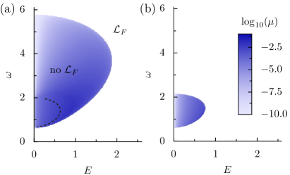
Figure 1: Distance from Markovianity $\mu$ of the effective generator of the one-cycle evolution superoperator as a function of driving strength $E$ and frequency $\omega$, for weak dissipation $\gamma=0.01$ and two driving phases (a) $\varphi=0$ and (b) $\varphi=\pi/2$. In the white region, where $\mu=0$, a Floquet Lindbladian $\mathcal{L}_{F}$ exists. On the dashed line the Floquet map $\mathcal{P}(T)$ possesses two negative real eigenvalues.

We can now distinguish three different possible scenarios for a given time-periodic Lindbladian $\mathcal{L}(t)$: (a) the action of $\mathcal{P}(T)$ can be reproduced with an effective (time-independent) Markovian master equation described by a time-independent generator of Lindblad form (Floquet Lindbladian) $\mathcal{L}_{F}$, $\mathcal{P}(T)=\exp(T\mathcal{L}_{F})$; (b) the action of $\mathcal{P}(T)$ is reproduced with an effective non-Markovian master equation characterized by a time-homogeneous memory kernel; (c) neither (a) nor (b), i.e. the action of $\mathcal{P}(T)$ cannot be reproduced with any time-homogeneous master equation. Scenario (a) is implicitly assumed in recent papers Haddadfarshi et al. (2015); Restrepo et al. (2016); Dai et al. (2016), where a high-frequency Floquet-Magnus expansion Blanes et al. (2009) (routinely used for isolated Floquet systems Goldman and Dalibard (2014); Bukov et al. (2015); Eckardt and Anisimovas (2015)) is employed in order to construct an approximate Floquet Lindbladian. It requires that at least one branch of the operator logarithm $\log\mathcal{P}(T)$ has to be of Lindblad form so that it can be associated with $T\mathcal{L}_{F}$. However, differently from the case of isolated systems, it is not obvious whether there is at least one valid branch for a given open Floquet system, since general CPTP maps do not always possess a logarithm of Lindblad type Wolf et al. (2008). Below we demonstrate that scenario (a) is not always realized even in the case of a simple two-level model. Instead, we find that the parameter space is shared by two phases corresponding to scenario (a) and (b), respectively.

We consider a two-level system described by a time-periodic Hamiltonian $H(t)$ and a single time-independent jump operator $A$,

$$H(t)=\frac{\Delta}{2}\sigma_{z}+E\cos(\omega t-\varphi)\sigma_{x}\text{ and }A=\sqrt{\gamma}\sigma_{-}.$$ (4)

Here $\sigma_{x}$, $\sigma_{z}$ and $\sigma_{-}$ are standard Pauli and lowering operators. Using the level splitting $\Delta$ and $\hbar/\Delta$ as units for energy and time (so that henceforth $\Delta=\hbar=1$), the model is characterized by four dimensionless real parameters: the dissipation strength $\gamma$ as well as the driving strength $E$, frequency $\omega$, and phase $\varphi$.

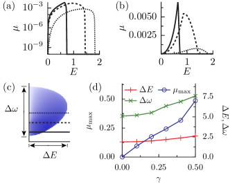
Figure 2: (a, b) Distance from Markovianity $\mu$ along horizontal cuts through the phase diagram of Fig. 1(a) for $\omega=1,2,3$ (solid, dashed, dotted line, cuts are shown in (c)). (d) Maximum extent of the non-Lindbladian phase with respect to frequency, $\Delta\omega$, and driving strength, $\Delta E$, (defined as we sketch in (c)) and maximum non-Markovianity $\mu_{\text{max}}=\max_{\omega,E}[\mu(\omega,E)]$ versus dissipation strength $\gamma$.

Let us first address the question of the existence of a Floquet Lindbladian. For an open system, $\gamma>0$, we have to consider the one-cycle evolution superoperator $\mathcal{P}(T)$ Szczygielski (2014); Hartmann et al. (2017). Since it is a CPTP map, its spectrum is invariant under complex conjugation. Thus, its $N^{2}$ eigenvalues are either real or appear as complex conjugated pairs (we denote the number of these pairs $n_{c}$). This Floquet map shall be diagonalized, $\mathcal{P}(T)=\sum_{a}\lambda_{a}\mathcal{M}_{a}=\sum_{r}\lambda_{r}\mathcal{M}_{r}+\sum_{c}(\lambda_{c}\mathcal{M}_{c}+{\lambda}^{*}_{c}\mathcal{{M}}_{c*})$, with $n_{c}$ pairs $\{\lambda_{c},{\lambda}^{*}_{c}\}$ and (not necessarily self-adjoint) projectors $\mathcal{M}_{a}$.

To find out whether we are in scenario (a), we implement the Markovianity test proposed by Wolf et al. in Refs. Wolf et al. (2008); Cubitt et al. (2012). Namely, in order to be consistent with a time independent Markovian evolution, $\mathcal{P}(T)$ should have at least one logarithm branch, $\mathcal{S}_{\{\mathbf{x}\}}=\frac{1}{T}\log\mathcal{P}(T)=\mathcal{S}_{0}+\frac{2\pi i}{T}\sum_{c=1}^{n_{c}}x_{c}(\mathcal{M}_{c}-\mathcal{{M}}_{c*})$, that gives rise to a valid Lindblad generator ($\mathcal{S}_{0}$ is the principal branch). Here a set of $n_{c}$ integers $\{\mathbf{x}\}=\{x_{1},...,x_{n_{c}}\}\in\mathbb{Z}^{n_{c}}$ labels a branch of the logarithm. To get the Floquet Lindbladian $\mathcal{L}_{F}$, we should find a branch for which the superoperator $\mathcal{S}_{\{\mathbf{x}\}}$ fulfills two conditions: (i) it should preserve Hermiticity and (ii) it has to be conditionally completely positive Evans (1977). Already here the contrast with the unitary case (where all branches provide a licit Floquet Hamiltonian) becomes apparent: it is not guaranteed that such branch exists. There is no need to inspect the different branches to check condition (i). It simply demands that the spectrum of $\mathcal{S}_{\{\mathbf{x}\}}$ has to be invariant under complex conjugation. This means, in turn, that the spectrum of the Floquet map $\mathcal{P}(T)$ should not contain negative real eigenvalues (or, strictly speaking, there must be no eigenvalues of odd degeneracy, whose integer powers give negative numbers). Condition (ii) is more complicated and involves properties of the spectral projectors $\mathcal{M}_{a}$ of the Floquet map. The corresponding test was formulated in Refs. Wolf et al. (2008); Cubitt et al. (2012) (we provide a brief operational description in the supplemental material SM ).

If the result of one of the two tests is negative and therefore no Floquet Lindbladian exists, it is instructive to quantify the distance from Markovianity by introducing some measure and then picking the branch $\mathcal{S}_{\{\mathbf{x}\}}$ giving rise to the minimal value of the measure. For this purpose, we compute two different measures for non-Markovianity proposed by Wolf et al. Wolf et al. (2008) and Rivas et al. Rivas et al. (2010). The first measure is based on adding a noise term $-\chi\mathcal{N}$ of strength $\chi$ to the generator and noting the minimal strength $\mu=\chi_{\text{min}}$ required to make it Lindbladian [so that it fulfills conditions (i) and (ii)]. Here $\mathcal{N}$ is the generator of the depolarizing map $\exp(T\chi\mathcal{N})\rho=\mathrm{e}^{-\chi T}\rho+[1-\mathrm{e}^{-\chi T}]\frac{\mathbb{1}}{N}$ Wolf et al. (2008); SM . The second measure quantifies the violation of positivity of the Choi representation Choi (1975); Jamiołkowski (1972); Holevo (2012) of the generated map SM ; Rivas et al. (2010). Interestingly, we find that for our model system both measures agree: within the numerical accuracy the second measure is always found to be equal to $\mu/2$.

In Fig. 1(a) we plot the distance from Markovianity $\mu$ for the effective generator of the one-cycle evolution superoperator $\mathcal{P}(T)$ versus driving amplitude $E$ and frequency $\omega$. We choose $\varphi=0$ and weak dissipation $\gamma=0.01$. The blue lobe, where $\mu>0$, corresponds to a phase, where a Floquet Lindbladian $\mathcal{L}_{F}$ does not exist. This non-Lindbladian phase is surrounded by a Lindbladian phase (white region) where $\mu=0$ so that $\mathcal{L}_{F}$ can be constructed [scenario (a)]. It contains also the $\omega$ axis, corresponding to the trivial undriven limit $E=0$. Note that only for a fine-tuned set of parameters, lying on the dashed line in Fig. 1(a), $\mathcal{P}(T)$ possesses negative eigenvalues. However, they come in a degenerate pair, such that the construction of a Floquet Lindbladian is not hindered by condition (i). Both the high- and the low-frequency limit are surrounded by finite frequency intervals, where the Floquet Lindbladian exists. This suggests that it might be possible to construct the Floquet Lindbladian in the high-frequency regime from a Floquet-Magnus-type expansion Haddadfarshi et al. (2015); Restrepo et al. (2016); Dai et al. (2016). Somewhat counter-intuitively, we find that the Floquet Lindbladian always exists for sufficiently strong driving strengths $E$, so that for large $E$ the low and the high-frequency Lindbladian phases are connected. However, for intermediate frequencies, a phase where no Floquet Lindbladian exists stretches over a finite interval of driving strengths $E$ separated only infinitesimally from the undriven limit $E=0$. This can also be seen from Fig. 2(a) and (b), where we plot $\mu$ along horizontal cuts through the phase diagram [indicated by the lines of unequal style in Fig. 2(c)] using a logarithmic and a linear scale, respectively.

Figure 1(b) shows the phase diagram for a different driving phase, $\varphi=\pi/2$. Remarkably, compared to $\varphi=0$ [Fig. 1(a)] the non-Lindbladian phase now covers a much smaller area in parameter space. The phase boundaries depend on the driving phase or, in other words, on when during the driving period we monitor the stroboscopic evolution of the system in a particular experiment. In the coherent limit, we can decompose the time evolution operator of a Floquet system from time $t_{0}$ to time $t$ like $U(t,t_{0})=U_{F}(t)\exp[-i(t-t_{0})H_{\text{eff}}]U_{F}^{\dagger}(t_{0})$, where $U_{F}(t)=U_{F}(t+T)$ is a unitary operator describing the time-periodic micromotion of the Floquet states of the system and $H_{\text{eff}}$ is a time-independent effective Hamiltonian. The Floquet Hamiltonian $H^{F}_{t_{0}}$, defined via $U(t_{0}+T,t_{0})=\exp(-iTH^{F}_{t_{0}})$ so that it describes the stroboscopic evolution of the system at times $t_{0}$, $t_{0}+T$, …, is for general $t_{0}$ then given by $H^{F}_{t_{0}}=U_{F}(t_{0})H_{\text{eff}}U_{F}^{\dagger}(t_{0})$ Eckardt and Anisimovas (2015). (Note that above we used the lighter notation $H_{F}=H^{F}_{0}$ for $t_{0}=0$.) It depends on the micromotion via a $t_{0}$-dependent unitary rotation. However, in the dissipative system the micromotion will no longer be captured by a unitary operator. This explains why the effective time-independent generator of the stroboscopic evolution can change its character as a function of $t_{0}$ (or, equivalently, the driving phase $\varphi$) in a nontrivial fashion, e.g. from Lindbladian to non-Lindbladian.

In Fig. 2(d), the dependence of the phase diagram on the dissipation strength $\gamma$ is investigated. We find that the extent of the non-Lindbladian phase both in frequency, $\Delta\omega$, and driving strength, $\Delta E$, [defined in Fig. 2(c)] does not vanish in the limit $\gamma\to 0$. Thus, even for arbitrary weak dissipation the Floquet Lindbladian does not exist in a substantial region of parameter space. It is noteworthy that the maximum distance from Markovianity $\mu$ goes to zero linearly with $\gamma$, i.e., the non-Markovianity is a first-order effect with respect to the dissipation strength.

While in the non-Lindbladian phase, we are not able to find a Markovian time-homogeneous master equation reproducing the one-cycle evolution operator $\mathcal{P}(T)$, one might still be able to construct a time-homogeneous non-Markovian master equation, which is non-local in time and described by a memory kernel Budini (2004); Breuer et al. (2016); Chruściński and Należyty (2016). In order to construct such an equation, we assume an evolution with an exponential memory kernel for $t\leq T$

$$\partial_{t}\tilde{\varrho}(t)=\frac{1}{\tau_{\text{mem}}}\int_{0}^{t}d\tau\,e^{(\tau-t)/\tau_{\text{mem}}}\mathcal{K}\tilde{\varrho}(\tau),$$ (5)

where $\tau_{\text{mem}}$ is the memory time and $\mathcal{K}$ the kernel superoperator. It is important to understand that a time-homogeneous master equation (5), when being integrated forward in time $t$ also beyond $T$, would not reproduce the same map after every period, since $\tilde{\mathcal{P}}(2T)$, $\tilde{\mathcal{P}}(3T)$, etc., will depend on the the corresponding pre-history of the length $2T$, $3T$, etc.. The stroboscopic evolution can only be obtained by erasing the memory after every period, which formally corresponds to multiplying the integrand of Eq. (5) by $\Theta\left(\tau-\lfloor t/T\rfloor T\right)$, where $\Theta$ and $\lfloor\cdot\rfloor$ denote the Heaviside step function and the floor function, respectively.

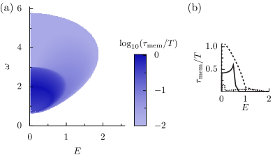
Figure 3: (a) Shortest memory time $\tau_{\text{mem}}$ for the exponential kernel of the effective non-Markovian generator in Eq. (5). $\tau_{\text{mem}}=0$ (white) indicates the Lindbladian phase. Due to limited numerical accuracy, we cannot resolve values of $\tau_{\mathrm{mem}}\leq 10^{-2}T$. This leads to a spurious plateau of apparently constant $\tau_{\text{mem}}=10^{-2}T$. Other parameters as in Fig. 1(a). (b) Cuts through the phase diagram at $\omega=1,2,3$ (solid, dashed, dotted line), similar to Fig. 2(b).

Let the map $\tilde{\mathcal{P}}$ describe the evolution resulting from the effective master equation (5), $\tilde{\varrho}(t)=\tilde{\mathcal{P}}(t)\varrho(0)$. It solves $\partial_{t}\tilde{\mathcal{P}}(t)={\tau}^{-1}_{\text{mem}}\int_{0}^{t}\mathrm{d}\tau\,e^{(\tau-t)/\tau_{\text{mem}}}\mathcal{K}\tilde{\mathcal{P}}(\tau)$ with $\tilde{\mathcal{P}}(0)=\mathbb{1}$. We now have to construct a superoperator $\mathcal{K}$, so that $\tilde{\mathcal{P}}(T)=\mathcal{P}(T)$. For that purpose, we represent the one-cycle evolution in its diagonal form, $\mathcal{P}(T)=\sum_{a}\lambda_{a}\mathcal{M}_{a}$. A natural ansatz is then $\mathcal{K}=\sum_{a}\eta_{a}\mathcal{M}_{a}$, for which we find an evolution operator of the form $\tilde{\mathcal{P}}(t)=\sum_{a}h_{a}(t)\mathcal{M}_{a}$, with characteristic decay functions $h_{a}(t)$ obeying $h_{a}(0)=1$. Plugging this ansatz into the equation of motion, the problem reduces to solving a set of scalar equations. They possess solutions SM $h_{a}(t)=\mathrm{e}^{-t/2\tau_{\text{mem}}}[\cosh(\Gamma_{a}t)+\sinh(\Gamma_{a}t)/(2\Gamma_{a}\tau_{\text{mem}})]$ with $\Gamma_{a}=[\tau_{\text{mem}}^{-2}/4+\tau_{\text{mem}}^{-1}\eta_{a}]^{1/2}$. Requiring $h_{a}(T)=\lambda_{a}$, determines the eigenvalues $\eta_{a}$ as a function of the memory time $\tau_{\text{mem}}$. It is then left to check, whether the corresponding $\mathcal{K}=\mathcal{K}(\tau_{\mathrm{mem}})$, which depends on the memory time $\tau_{\text{mem}}$, gives rise to an evolution that is CPTP at all times $t$. Note that in contrast to the Markovian limit, $\tau_{\text{mem}}\to 0$, where $\mathcal{K}$ needs to be of Lindblad form, for finite memory time $\tau_{\text{mem}}$ it is an intriguing open question to find general conditions that characterize the admissible superoperators $\mathcal{K}$ that give rise to an evolution that is CPTP. Ideas to characterize special cases Budini (2004); Maniscalco (2007); Siudzińska and Chruściński (2017, 2019); Wudarski et al. (2015) have been developed but unfortunately are not directly applicable to our problem. Even though general sufficient conditions exist Chruściński and Kossakowski (2016), it is unclear how to bring Eq. (5) into a form that is required to prove these conditions.

In the absence of a general criterion, we perform a numerical test to check whether $\tilde{\mathcal{P}}(t)$ is completely positive. The test is based on the fact that a given map $\mathcal{P}$ is completely positive if and only if its Choi representation is positive, $\mathcal{P}^{\Gamma}=(\mathcal{P}\otimes\rm id){\left|\Omega\right\rangle}{\left\langle\Omega\right|}\geq 0$ Choi (1975); Jamiołkowski (1972), where ${\left|\Omega\right\rangle}=\frac{1}{\sqrt{2}}\left({\left|00\right\rangle}+{\left|11\right\rangle}\right)$ is a maximally entangled state of the system and an ancilla of the same size. Thus, we require positivity of the Choi representation, $\tilde{\mathcal{P}}(t_{n})^{\Gamma}\geq 0$, for all times $t_{n}\in[0,T]$ on a numerical grid with 100 intermediate steps. Note that, because of the memory erasure after every period, we do not impose the CPTP condition on the maps generated by the pair $\{\mathcal{K}(\tau_{\text{mem}}),\tau_{\text{mem}}\}$ for times $t>T$.

For all parameters, we find a memory time $\tau_{\text{mem}}$ such that $\mathcal{K}$ gives rise to an evolution that is CPTP. In the phase, where the Floquet Lindbladian $\mathcal{L}_{F}$ exists, we find a kernel $\mathcal{K}$ which yields a CPTP evolution for arbitrarily short memory times $\tau_{\text{mem}}$. In contrast, in the non-Lindbladian phase the memory time $\tau_{\text{mem}}$ cannot be smaller than some minimal value. In Fig. 3(a) we plot this minimal memory time versus driving strength and frequency. The resulting map shows good qualitative agreement with the distance to Markovianity $\mu$ shown in Fig. 1(a) (the apparent plateau of constant $\tau_{\text{mem}}=10^{-2}T$ is an artifact related to the fact that our numerical implementation is not able to resolve memory times smaller than $10^{-2}T$). Nevertheless, in contrast to the measure $\mu$, $\tau_{\text{mem}}$ does not tend to zero for small $E$ as we observe in Fig. 3(b). It is possible that a different behavior of $\tau_{\text{mem}}$ would be found for a more general ansatz of the memory kernel. The specific form of our ansatz implies that the minimal memory time found here provides an upper bound for the minimal memory time for general time-homogeneous memory kernels only. Note that the memory time $\tau_{\mathrm{mem}}$ can even be larger than $T$.

Interestingly, we find that in the regime of large memory times $\tau_{\text{mem}}$, the minimal memory time is found for a Kernel operator $\mathcal{K}$ of Lindblad form. At first this seems counter-intuitive because Eq. (5) gives rise to a Markovian evolution in the opposite limit, $\tau_{\mathrm{mem}}\to 0$. However one can show SM $\tilde{\mathcal{P}}(t)\approx\exp({\mathcal{K}}t^{2}/{2\tau_{\mathrm{mem}}})$ for $t\ll\tau_{\mathrm{mem}}$, which is a quantum semigroup with rescaled time $t^{\prime}=t^{2}$. Thus, the map $\tilde{\mathcal{P}}(t)$ is guaranteed to become CPTP in the limit $t/\tau_{\text{mem}}\to 0$ for a Lindbladian Kernel $\mathcal{K}$ and can be expected to remain CPTP also for a significant fraction of the period where $t/\tau_{\text{mem}}\ll 1$.

Finally, the fact that for the used model, we can always construct a time-homogeneous memory kernel which yields a CPTP evolution on the time interval $[0,T]$, means that the non-Lindbladian phase in this case corresponds to scenario (b). Nevertheless, let us stress that the stroboscopic action of $\mathcal{P}(nT)$ over more than one period (i.e. not only for $n=1$, but also for all $n\geq 2$) can in general not be obtained from an effective time-homogeneous non-Markovian evolution like in Eq. (5), but with $t$ taking also values $t>T$, because it is essential that the memory is erased at stroboscopic instances of time.

Our results shed light on limitations and opportunities for Floquet engineering in open quantum systems. Using a simple model system, we have shown that an effective Floquet Lindbladian generator, constructed analogously to the Floquet Hamiltonian for isolated Floquet systems, exists in extensive parameter regimes. In particular for sufficiently large driving frequencies the Floquet Lindbladian can be constructed, suggesting that here high-frequency approximation schemes Haddadfarshi et al. (2015); Restrepo et al. (2016); Dai et al. (2016) should indeed be applicable (even though it is an open question whether or when these give rise to the correct Lindbladian effective generator). However, we found also an extended parameter region, where it does not exist, and where only a time-homogeneous non-Markovian effective master equation is able to reproduce the one-cycle evolution. This finding poses an intriguing question as to whether time-dependent Markovian systems can be used – in a controlled fashion – to mimic non-Markovian ones. Another relevant observation is that the existence of the Floquet Lindbladian depends on when during the driving period the model is stroboscopically monitored. This reveals an important role played by the non-unitary micromotion in open Floquet systems, which we might hope to exploit for the purpose of dissipative Floquet engineering, and which may as well be important in the context of quantum heat engines Scopa et al. (2018). In future work, it will be crucial to develop intuitive approximation schemes allowing to tailor the properties of open Floquet systems. Also, the behavior of larger systems has to be investigated (though from the computational point of view it is a very hard problem; see, e.g., Ref. Hartmann et al. (2017) for a first study in this direction).