Transit Timing Variations and linear ephemerides of confirmed Kepler transiting exoplanets

Abstract

We determined new linear ephemerides of transiting exoplanets using long-cadence de-trended data from quarters Q1 to Q17 of Kepler mission. We analysed TTV diagrams of 2098 extrasolar planets. The TTVs of 121 objects were excluded (because of insufficient data-points, influence of stellar activity, etc). Finally, new linear ephemerides of 1977 exoplanets from Kepler archive are presented. The significant linear trend was observed on TTV diagrams of approximately 35% of studied exoplanets. Knowing correct linear ephemeris is principal for successful follow-up observations of transits. Residual TTV diagrams of 64 analysed exoplanets shows periodic variation, 43 of these TTV planets were not reported yet.

1 Introduction

The Kepler satellite, launched in 2009, provided during its primary mission high-precision, high-cadence and continuous photometric data (Borucki et al., 2010). After losing two reaction wheels in 2013, so-called K2 mission started and still continue (Howell et al., 2014).

During the primary mission, Kepler discovered 2327 extrasolar planets (up to May 31^st, 2018). Almost the half of them (1125) are located in 447 multi-planet systems. The final catalogue (DR25) of Kepler planet candidate was released in 2017 (Thompson et al., 2018). It consists of more than four thousand of planet candidates.

In many of known exoplanets, the variations in times of transits were already observed. Holczer et al. (2016) detected 260 planet candidates with significant long-term variations. These variations could be caused by gravitational interaction with another bodies in the system. For example, Steffen et al. (2012) determined the masses of planets in the systems Kepler-25, Kepler-26, Kepler-27 and Kepler-28 using transit timing. Similar method is also used to confirm the planets in multi-planetary systems (e.g. Fabrycky et al. (2012)). Many of planet pairs are captured into mean motion resonances (MMRs) (Wang & Ji, 2017). The MMRs 3:2 and 2:1 are the most common(Wang & Ji, 2014).

Table 1: The new linear ephemerides of Kepler exoplanets: Kepler, KOI (Kepler Object of Interest) and KIC (Kepler Input Catalog ) - name of exoplanet, $P$ - orbital period, $T_{0}$ - an initial time of transit (uncertainties are given in parenthesis), $\chi^{2}$ - sum of squares of the best fit, $\chi^{2}/n$ - reduced sum of squares, $n$ - number of data points in TTV diagram, Note - changes of residual TTV after new ephemeris is removed, 1 - no significant changes, 2 - periodic or quasi-periodic variations, 3 - chaotic variations (see text for a detailed description). The full table is available as a supplementary material to this manuscript.

Names			New ephemeris		Fit statistics			Note
Kepler	KOI	KIC	$P$ (d)	$T_{0}$ (BJD)	$\chi^{2}$	$\chi^{2}/n$	$n$
Kepler-4 b	7.01	11853905	3.213663(1)	2454956.61167(24)	523.9	1.6	330	1
Kepler-5 b	18.01	8191672	3.5484659(1)	2454955.90135(3)	6020.5	16.0	379	1
Kepler-6 b	17.01	10874614	3.2346994(8)	2454954.48659(2)	5598.0	16.8	335	1
…	…	…	…	…	…	…	…	…
Kepler-1646 b	6863.01	7350067	4.485563(2)	2454968.43834(30)	9126.425	31.579	291	1

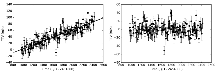
Figure 1: TTV of Kepler-114 c determined from original ephemeris from NASA Exoplanet Archive with new linear fit (solid line), $right$ – residual TTV of Kepler-114 c (note 1 in Table 1).

2 Linear ephemeris determination

In our analysis we used long-cadence (sampled every 29.4 minutes) de-trended data (PDCSAP_FLUX) from quarters Q1 to Q17 of Kepler mission, obtained from Mikulski Archive for Space Telescopes (MAST). For the analysis of data, we used the same pipeline as in our study of transit-timing variations (TTVs) in the system Kepler-410 (Gajdoš et al., 2017). We used same approach for all studied planets and got homogeneous set of times of transits by one method. It can be summarized in the following steps:

1. Parts of the light curve (LC) of the individual system were extracted around detected transits (using ephemeris given by NASA Exoplanet Archive (Akeson et al., 2013)), with an interval two times bigger than the transit duration.

2. Additional residual trends caused by the stellar activity and/or instrumental long-term photometric variation were removed by the fitting out-of-transit part of LC by the second-order polynomial function.

3. All individual parts of the LC with transits were stacked together. This can be done, because one expects that the physical parameters of the host star and the exoplanet did not change during the observational period of about 3.5 years and we want to cancel-out the effect of stellar activity.

4. Stacked LC was fitted by our software implementation of Mandel & Agol (2002) model where we used a quadratic model of limb darkening with values of coefficients from Sing (2010). Our package use Markov Chain Monte-Carlo (MCMC) simulation to obtain statistically significant value of parameters and their errors.

5. Obtained template was used to fit all individual transits, where only the time of transit was updated.

6. Determined times of transits were used for a creation of transit timing variations (TTV) diagram of the object. It was subsequently fitted by the linear function to obtain new values of linear ephemeris parameters, initial time of transit $T_{0}$ and orbital period $P$. To achieve statistically significant estimation of parameter’s uncertainties, we used MCMC simulation. To estimate the quality of the statistical model, we have calculated sum of squares $\chi^{2}$ and reduced sum of squares $\chi^{2}/n$ where $n$ is the number of data points in TTV diagram.

7. Finally, new linear trend determined by new ephemeris was removed and residual TTV was visually inspected for another changes.

Table 2: Comparison of periods and amplitudes of TTV changes found in this paper with values given by Holczer et al. (2016): Kepler, KOI and KIC - name of exoplanet, $P$ - period of variation, $A$ - amplitude (uncertainties are given in parenthesis).

Names			Holczer et al. (2016)		This paper
Kepler	KOI	KIC	$P$ (d)	$A$ (m)	$P$ (d)	$A$ (m)
Kepler-25 b	244.02	4349452	326(3)	3.8(3)	334(2)	4.3(3)
Kepler-51 b	620.01	11773022	790(12)	7.9(4)	749(17)	5.5(5)
Kepler-81 c	877.02	7287995	536(12)	9(2)	516(9)	10(1)
Kepler-111 c	139.01	8559644	2213(79)	211(22)	1050(20)	38(2)
Kepler-139 c	316.02	8008067	1008(84)	29(8)	913(30)	35(3)
Kepler-209 c	672.02	7115785	1061(76)	9(2)	1141(63)	10(1)
Kepler-221 e	720.03	9963524	—	$\sim$9	1697(115)	11(1)
Kepler-278 c	1221.02	3640905	829(41)	144(32)	960(69)	112(16)
Kepler-312 c	1628.01	6975129	471(17)	6(2)	478(14)	7(1)
Kepler-359 c	2092.01	6696580	1270(130)	23(6)	1246(125)	20(6)
Kepler-540 b	374.01	8686097	1388(84)	38(6)	1457(54)	37(4)
Kepler-561 b	464.01	8890783	482(11)	3.9(6)	480(12)	4.1(7)
Kepler-591 b	536.01	10965008	454(37)	6(4)	579(35)	9(2)
Kepler-765 b	1086.01	10122255	1630(150)	20(4)	1445(133)	37(3)
Kepler-827 b	1355.01	7211141	124(1)	6(2)	398(36)	6(1)
Kepler-1040 b	1989.01	10779233	—	$\sim$15	901(30)	17(4)
Kepler-1624 b	4928.01	1873513	110(1)	2.1(7)	118(3)	1.9(2)

Table 3: Planets with periodic variations in TTV diagram not reported in Holczer et al. (2016).

Names			Variation
Kepler	KOI	KIC	$P$ (d)	$A$ (m)
Kepler-39 b	423.01	9478990	1393(81)	1.9(3)
Kepler-52 d	775.03	11754553	1493(300)	9(4)
Kepler-89 c	94.02	6462863	395(10)	10(2)
Kepler-110 b	124.01	11086270	767(23)	12(4)
Kepler-110 c	124.02	11086270	1245(13)	6(2)
Kepler-122 e	232.04	4833421	1135(59)	42(6)
Kepler-142 d	343.03	10982872	1400(5)	57(9)
Kepler-166 c	481.03	11192998	1419(81)	20(5)
Kepler-196 c	612.02	6587002	1431(197)	7(1)
Kepler-201 c	655.02	5966154	828(88)	11(4)
Kepler-222 d	723.02	10002866	770(23)	5(1)
Kepler-222 c	723.03	10002866	606(11)	3.2(5)
Kepler-227 c	752.02	10797460	1041(12)	14(8)
Kepler-230 c	759.02	11018648	776(60)	19(6)
Kepler-233 c	790.02	12470844	1057(127)	12(5)
Kepler-267 d	1078.03	10166274	818(24)	8(2)
Kepler-283 c	1298.02	10604335	1212(36)	68(11)
Kepler-299 e	1432.04	11014932	1427(102)	74(46)
Kepler-300 c	1435.01	11037335	1365(104)	58(10)
Kepler-310 c	1598.01	10004738	1004(10)	5(2)
Kepler-310 b	1598.03	10004738	1134(49)	15(3)
Kepler-358 c	2080.01	10864531	810(3)	19(6)
Kepler-362 c	2147.01	10404582	851(85)	14(6)
Kepler-364 c	2153.01	10253547	696(66)	23(4)
Kepler-509 b	276.01	11133306	1506(138)	4(1)
Kepler-549 c	427.03	10189546	978(43)	42(8)
Kepler-672 b	773.01	11507101	707(32)	14(3)
Kepler-795 b	1218.01	3442055	731(27)	10(4)
Kepler-797 b	1238.01	6383821	895(60)	37(11)
Kepler-807 b	1288.01	10790387	1327(97)	1.8(5)
Kepler-852 b	1444.01	11043167	1123(76)	15(3)
Kepler-966 b	1828.01	11875734	1162(120)	7(2)
Kepler-1036 b	1980.01	11769890	1382(84)	16(2)
Kepler-1097 b	2102.01	7008211	729(29)	9(1)
Kepler-1126 b	2162.01	9205938	1327(133)	23(6)
Kepler-1129 c	2167.03	6041734	1236(117)	19(4)
Kepler-1184 b	2309.01	10010440	1108(51)	24(5)
Kepler-1185 b	2311.03	4247991	820(89)	9(3)
Kepler-1388 b	2926.01	10122538	370(19)	18(7)
Kepler-1389 b	2931.01	8611257	1312(101)	43(8)
Kepler-1453 b	3280.01	10653179	1078(2)	22(10)
Kepler-1524 b	3878.01	4472818	974(77)	4(1)
Kepler-1527 b	3901.01	9480535	1024(25)	44(5)
Kepler-1530 c	3925.03	10788461	86.4(6)	13(3)
Kepler-1552 b	4103.01	3747817	998(125)	28(8)
Kepler-1593 b	4356.01	8459663	1465(134)	28(9)
Kepler-1638 b	5856.01	11037818	840(51)	197(32)

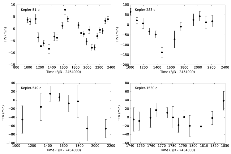
Figure 2: Examples of planets with periodic variations on the residual TTV diagram (note 2 in Table 1). Periods and amplitudes of these changes are listed in Tables 2 and 3.

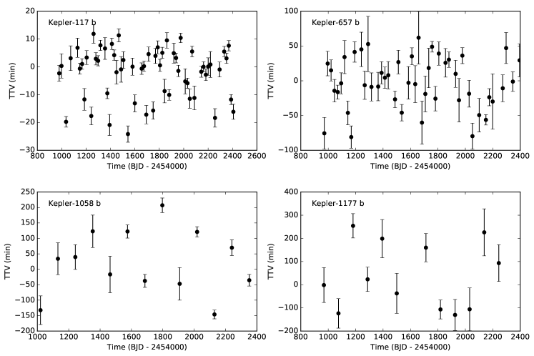
Figure 3: Examples of exoplanets with chaotic (abnormal) TTVs (note 3 in Table 1).

3 Discussion and conclusion

We started our analysis of TTV diagrams with 2098 extrasolar planets from Kepler database. We excluded 121 objects with TTV diagrams consisting less than 4 points or with diagrams strongly affected by stellar activity. New linear ephemeris were determined for 1977 exoplanets. They are all presented in Table 1.

Our analysis revealed that in many cases ($\sim 35\%$), linear trend could be observed on the TTV diagrams which were calculated according to original ephemerides given by NASA Exoplanet Archive. Cumulative shift in the minima times of studied exoplanets can reach up to $\sim 130$ minutes (e.g. Kepler-4 b) over 3.5 years of Kepler observations. The example of such a significant trend detected in the system Kepler-114 c is shown on Fig. 1 (left). The period of Kepler-114 c given by the NASA Exoplanet Archive is 8.041 days. But the reference (Xie, 2014) for it is quite old and had used only data up to Q16 quarter. We used also Q17 data in this paper. Also in many other cases, the ephemeris given by the Archive is not the latest one. The incorrect value of period could cause that the transit will be really observed few hours earlier or latter than it will be calculated, after few years. And the observer with outdated ephemeris will not see any transit at all. After removing linear trend determined by the new ephemeris, we can obtain residual TTV with no other significant changes (right) (note 1 in Table 1).

Residual TTV of 64 planets shows periodic or quasi-periodic variations (note 2 in Table 1). The examples of such systems with more or less significant changes are depicted in Fig. 2. TTV of 17 planets from this group were already analysed by Holczer et al. (2016). We compared our results with their in the Table 2. Periodic TTV signals of six planets (Kepler-52 d, Kepler-89 c, Kepler-122 e, Kepler-166 c, Kepler-283 c and Kepler-549 c) were already reported by Thompson et al. (2018) but they did not determine any parameters of these changes. 43 of these planets with periodic TTV were not reported in any other paper. Discovering these new TTV systems was a result of using our method of LC de-trending and time of transit measurement. The all planets with unreported periodic TTV and six planets reported (but not analysed) by Thompson et al. (2018) are listed in Table 3 with periods and amplitudes of TTV changes. We used sinusoidal model of these variations to determined their period and amplitude. For finding correct values of sinusoidal model’s parameters, we ran simple Levenberg-Marquardt algorithm (Marquardt, 1963). Amplitudes of found variations vary between approximately 2 and 70 minutes and periods vary from only 80 to more than 1500 days. These changes could be caused by interaction with another body(ies) (e.g. Agol et al. (2005)), stellar activity (e.g. spots) or other effects in studied systems.

95 exoplanets shows chaotic or abnormal TTVs (note 3 in Table 1). This type of variations is the most probably caused by stellar activity (e.g. Oshagh et al. (2013)) and/or gravitational interaction with another bodies in the systems. Examples of these systems are shown on Figure 3.

Supporting information

Additional Supporting Information may be found in the on-line version of this article:
Table 1. The new linear ephemeris of Kepler exoplanets.

References

- Agol et al. (2005) Agol, E., Steffen, J., Sari, R., & Clarkson, W. 2005, MNRAS, 359, 567
- Akeson et al. (2013) Akeson, R. L., Chen, X., Ciardi, D., et al. 2013, PASP, 125, 989
- Borucki et al. (2010) Borucki, W. J., Koch, D., Basri, G., et al. 2010, \sci, 327, 977
- Fabrycky et al. (2012) Fabrycky, D. C., Ford, E. B., Steffen, J. H., et al. 2012, ApJ, 750, 114
- Gajdoš et al. (2017) Gajdoš, P., Parimucha, Š., Hambálek, Ľ., & Vaňko, M. 2017, MNRAS, 469, 2907
- Holczer et al. (2016) Holczer, T., Mazeh, T., Nachmani, G., et al. 2016, ApJS, 225, 9
- Howell et al. (2014) Howell, S. B., Sobeck, C., Haas, M., et al. 2014, PASP, 126, 398
- Mandel & Agol (2002) Mandel, K., & Agol, E. 2002, ApJ, 580, L171
- Marquardt (1963) Marquardt, D. 1963, SIAM J Appl Math, 11, 431
- Oshagh et al. (2013) Oshagh, M., Santos, N. C., Boisse, I., et al. 2013, A&A, 556, A19.
- Sing (2010) Sing, D. K. 2010, A&A, 510, A21
- Steffen et al. (2012) Steffen, J. H., Fabrycky, D. C., Ford, E. B., et al. 2012, MNRAS, 421, 2342
- Thompson et al. (2018) Thompson, S. E., Coughlin, J. L., Hoffman, K., et al. 2018, ApJS, 235, 38.
- Wang & Ji (2014) Wang, S., & Ji, J. 2014, ApJ, 795, 85
- Wang & Ji (2017) Wang, S., & Ji, J. 2017, AJ, 154, 236
- Xie (2014) Xie, J.-W. 2014, ApJS, 210, 25