Shifted CholeskyQR for computing the QR factorization of ill-conditioned matrices

Abstract

The Cholesky QR algorithm is an efficient communication-minimizing algorithm for computing the QR factorization of a tall-skinny matrix. Unfortunately it has the inherent numerical instability and breakdown when the matrix is ill-conditioned. A recent work establishes that the instability can be cured by repeating the algorithm twice (called CholeskyQR2). However, the applicability of CholeskyQR2 is still limited by the requirement that the Cholesky factorization of the Gram matrix runs to completion, which means it does not always work for matrices $X$ with $\kappa_{2}(X)\gtrsim{{\bf u}}^{-\frac{1}{2}}$ where ${{\bf u}}$ is the unit roundoff. In this work we extend the applicability to $\kappa_{2}(X)=\mathcal{O}({\bf u}^{-1})$ by introducing a shift to the computed Gram matrix so as to guarantee the Cholesky factorization $R^{T}R=A^{T}A+sI$ succeeds numerically. We show that the computed $AR^{-1}$ has reduced condition number $\leq{{\bf u}}^{-\frac{1}{2}}$, for which CholeskyQR2 safely computes the QR factorization, yielding a computed $Q$ of orthogonality $\|Q^{T}Q-I\|_{2}$ and residual $\|A-QR\|_{F}/\|A\|_{F}$ both $\mathcal{O}({{\bf u}})$. Thus we obtain the required QR factorization by essentially running Cholesky QR thrice. We extensively analyze the resulting algorithm shiftedCholeskyQR3 to reveal its excellent numerical stability. shiftedCholeskyQR3 is also highly parallelizable, and applicable and effective also when working in an oblique inner product space. We illustrate our findings through experiments, in which we achieve significant (up to x40) speedup over alternative methods.

65F30, 15A23, 65F15, 15A18, 65G50

1 Introduction

Computing the QR factorization $X=QR$ is required in various applications in scientific computing. The Cholesky QR algorithm computes the factorization by:

(1) $$A=X^{\top}X,$$

(2) $$R=\mbox{chol}(A),$$

(3) $$Q=XR^{-1},$$

where $\mbox{chol}(A)$ denotes the Cholesky factor of $A$. Cholesky QR is a communication-avoiding algorithm whose communication cost is equivalent to that of the TSQR algorithm, which has been devised specifically to reduce communication for the QR factorization of tall-skinny matrices [3]. Cholesky QR has the advantage over TSQR that its arithmetic cost is about half and that its reduction operator is addition, while that of TSQR is a QR factorization of a small matrix [4]. As a result, Cholesky QR usually runs faster than TSQR. However, Cholesky QR is rarely used in practice because of its instability: the distance from orthogonality of its computed $Q$ grows rapidly with the condition number of the input matrix. By contrast, TSQR is unconditionally stable.

A recent work by the authors [16] establishes that the instability can be cured significantly by repeating the algorithm twice (called CholeskyQR2). However, the applicability of CholeskyQR2 is still limited by the requirement that the Cholesky factorization of the Gram matrix runs to completion, which means it does not always work for matrices $A$ with $\kappa_{2}(X)=\mathcal{O}({{\bf u}}^{-\frac{1}{2}})$ or larger, where ${\bf u}$ is the unit roundoff. In this work we extend the applicability of CholeskyQR-based algorithms to $\kappa_{2}(X)=\mathcal{O}({\bf u}^{-1})$.

The idea is to execute a preconditioning step so that the conditioning is improved to a point where CholeskyQR2 is applicable. How do we find an effective preconditioner? An inspiration to answer this is the fact that Cholesky QR and CholeskyQR2 belong to the category of triangular orthogonalization type algorithms [15, Lecture 10], in contrast to Householder type algorithms, which follows the principle of orthogonal triangularization. We summarize the classification of algorithms in terms of their principle, communication cost, and stability in Figure 2, which also clarifies where our contribution (shifted CholeskyQR3) stands.

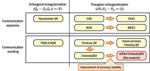
Figure 1: Classification of QR factorization algorithms.

In triangular orthogonalization, one right-multiplies an appropriate upper triangular matrix $R$ so that $\kappa_{2}(AR)=1$. Now, what if our goal is merely $\kappa_{2}(AR)=O({\bf u}^{-1/2})$? Once we have this, we can safely compute the QR factorization $AR=QR_{1}$ using CholeskyQR2, to arrive at the overall QR factorization $A=Q(R_{1}R^{-1})$.

Clearly, such $R$ is not unique, and we propose one way of finding such $R$. Namely, as in Cholesky QR we compute the Gram matrix, but add a small shift $sI$ so as to guarantee the Cholesky factorization $R^{T}R=A^{T}A+sI$ does not break down numerically. We show that under the mild assumption $\kappa_{2}(A)\leq{\bf u}^{-1}$, the resulting $AR^{-1}$ (note that $R^{-1}$ is also triangular) has reduced condition number $\leq{{\bf u}}^{-\frac{1}{2}}$, for which CholeskyQR2 safely computes the QR factorization, yielding computed $Q,R$ with excellent orthogonality $\|Q^{T}Q-I\|=\mathcal{O}({{\bf u}})$ and residual $\|A-QR\|_{F}/\|A\|_{F}=\mathcal{O}({{\bf u}})$, overall a backward stable QR factorization. The algorithm is deceptively simple (essentially the only new ingredient being the introduction of a shift); the analysis is however not trivial. We give detailed analysis that gives the constants hidden in the $\mathcal{O}({\bf u})$ notation.

The main message of this paper is that for any matrix with condition number well above ${{\bf u}^{-\frac{1}{2}}}$ (but bounded by ${{\bf u}^{-1}}$), the QR factorization can be computed in a backward stable manner by essentially running Cholesky QR thrice. We refer to this overall algorithm as shiftedCholeskyQR3; Figure 2 shows its diagram, and how $\kappa_{2}(A)$ is reduced eventually to 1 through repeated multiplication by triangular matrices.

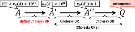
Figure 2: Diagram illustrating shiftedCholeskyQR3.

Let us comment on related studies in the literature. A recent work of Yamazaki et al. [18] uses doubled precision arithmetic (e.g., quadruple precision when using double precision) for the first two steps (1), (2), and shows that the condition number gets reduced by about $O({{\bf u}}^{-1})$, and thus the QR factorization will be obtained by repeating the process. This results in about 8.5 times as many arithmetic operations (per iteration) as does the standard CholeskyQR without doubled precision. Moreover, this approach clearly requires that higher-precision arithmetic is available, which may not always be the case (and even when it is, it often comes with a significant price in speed). shiftedCholeskyQR3 developed in this paper does not require change of arithmetic precision (in our experiments we use only IEEE double precision in which ${{\bf u}}\approx 1.1\times 10^{-16}$), and requires just one more CholeskyQR iteration than [18], thus is usually much faster.

As a bonus, our development is straightforward to apply to computing the QR factorization in a non-standard inner product space induced by a positive definite matrix $B\succ 0$, in which $(x,y)_{B}=x^{T}By$. Available algorithms for this task include (modified) Gram-Schmidt [12], and Cholesky QR [10, 14, 9]. A recent work by Lowery and Langou [10] studies the numerical stability, with no method apparently being (near) optimal in both orthogonality and backward error. We analyze the stability of shiftedCholeskyQR3 in this case to show it has favorable stability properties. Moreover, shiftedCholeskyQR3 is significantly faster than Gram-Schmidt type algorithms, achieving up to 40-fold speedup in our experiments with sparse $B$.

This paper is organized as follows. In Section 2 we describe the shiftedCholeskyQR algorithm. Section 3 analyzes shiftedCholeskyQR in detail and shows that it can be used to reduce $\kappa_{2}(X)$. In Section 4 we combine shiftedCholeskyQR and CholeskyQR2 to derive shiftedCholeskyQR3 for ill-conditioned matrices with $\kappa_{2}(X)=\mathcal{O}({\bf u}^{-1})$ and prove its backward stability. Section 5 discusses the extension to the non-standard inner product space. Numerical experiments are shown to illustrate the results in Section 6 and Section 7 summarizes the performance of our software implementations.

We primarily focus on real matrices $A\in\mathbb{R}^{m\times n}$, but everything carries over to complex matrices $A\in\mathbb{C}^{m\times n}$. We assume $m\geq n$, and the algorithms developed here are particularly useful in the tall-skinny case $m\gg n$.

2 Shifted Cholesky QR

To overcome the numerical breakdown in the Cholesky factorization (2), we propose a simple remedy: introduce a small shift $A^{T}A+sI$ to force the computed Gram matrix $A^{T}A$ to be numerically positive definite, so that its Cholesky factorization runs without breakdown. The rest of the algorithm is the same as Cholesky QR, and the algorithm shiftedCholeskyQR can be summarized in pseudocode in Algorithm 1.

Algorithm 1 shiftedCholeskyQR for $X=QR$

1:  $A=X^{\top}X,$

2:  choose $s>0$

3:  $R=\mbox{chol}(A+sI)$

4:  $Q=XR^{-1}$

Introducing shifts in Cholesky QR was briefly mentioned in [14], also as a remedy for the breakdown. However, the focus there was on the algorithm called SVQB, which computes the SVD of the Gram matrix instead of the Cholesky factorization. SVQB computes a factorization of the form $A=QB$, where $B$ is a full $n\times n$ matrix. While $Q$ is still a basis for the column space of $A$, an additional QR factorization of $B$ is needed to obtain a complete QR factorization of $A$. Furthermore, experiments suggest that there are benefits in working with a triangular matrix as in Cholesky QR as opposed to full matrices as in SVQB, wirh respect to the row-wise stability of the computed decomposition.

We shall discuss an appropriate choice of the shift $s$, which will be $O({\bf u})$, and prove that applying shiftedCholeskyQR to a matrix $X$ with ${\bf u}^{-\frac{1}{2}}<\kappa_{2}(X)<{\bf u}^{-1}$ results in a computed $\tilde{Q}$ with much reduced condition number $\kappa_{2}(\tilde{Q})<{{\bf u}}^{-\frac{1}{2}}$, for which CholeskyQR2 suffices to compute the QR factorization.

3 Convergence and stability analysis of shiftedCholeskyQR

In this section we present the main technical analysis of shiftedCholeskyQR. The goal is to show that the algorithm improves the conditioning significantly, that is, $\kappa_{2}(\tilde{Q})\ll\kappa_{2}(X)$.

A few assumptions need to be made on the matrix size and condition number. The constants below are not of significant importance but chosen so that the forthcoming analysis runs smoothly. We shall assume the following hold:

(4) $$6n^{2}{{\bf u}}\kappa_{2}(X)<1,$$

(5) $$mn{{\bf u}}\leq\frac{1}{64},$$

(6) $$n(n+1){{\bf u}}\leq\frac{1}{64},$$

(7) $$11\{mn+n(n+1)\}{{\bf u}}\|X\|_{2}^{2}\leq s\leq\frac{1}{100}\|X\|_{2}^{2}.$$

Roughly speaking, the first three assumptions require that the condition number $\kappa_{2}(X)$ is safely bounded above by ${{\bf u}^{-1}}$, and the matrix dimensions $m,n$ are small compared with the precision ${\bf u}^{-1}$. We reiterate that $\kappa_{2}(X)>{\bf u}^{-\frac{1}{2}}$ is allowed, a crucial difference from CholeskyQR2 treated in [16]. The assumption (7) imposes that $s$ is large enough for Cholesky to work, but small compared with $\|X\|_{2}^{2}$.

Note that by (5), (6) we have

(8) $$\gamma_{m}:=\frac{m{{\bf u}}}{1-m{{\bf u}}}\leq 1.02m{{\bf u}},\quad\gamma_{n+1}:=\frac{(n+1){{\bf u}}}{1-(n+1){{\bf u}}}\leq 1.02(n+1){{\bf u}}.$$

3.1 Preparations

We denote the computed quantities in shiftedCholeskyQR, accounting for the numerical errors, by

(9) $$\hat{A} = X^{\top}X+E_{1},$$

(10) $$\hat{R}^{\top}\hat{R} = \hat{A}+sI+E_{2}\;=\;X^{\top}X+sI+E_{1}+E_{2},$$

(11) $$\hat{q}_{i}^{\top} = x_{i}^{\top}(\hat{R}+\Delta\hat{R}_{i})^{-1}\quad(i=1,2,\dots m).$$

$\hat{q}_{i}^{\top}$, $x_{i}^{\top}$ are the $i$th rows of $X$ and $\hat{Q}$ respectively. $E_{1}$ is the matrix-matrix multiplication error in the computation of the Gram matrix $X^{\top}X$, and $E_{2}$ is the $\hat{A}$ backward error incurred when computing the Cholesky factorization. $\Delta\hat{R}_{i}$ is the backward error involved in the solution of the linear system $q_{i}^{\top}\hat{R}=x_{i}^{\top}$.

We shall take $s$ so that

(12) $$\|E_{1}\|_{2},\|E_{2}\|_{2}=o(s),$$

which means $s=c\max(\|E_{1}\|_{2},\|E_{2}\|_{2})$ for some $c>1$. In fact we shall see that $\|E_{1}\|_{2},\|E_{2}\|_{2}=O({\bf u})\|X\|^{2}_{2}$, so (12) simply means $s$ is chosen to be safely larger than ${\bf u}\|X\|^{2}_{2}$ (qualitatively this is also assumed by (11)). In particular, we write

(13) $$s:=\alpha\|X\|^{2}_{2},\quad 0<\alpha<1.$$

(11) gives

$$\hat{q}_{i}^{\top}=x_{i}^{\top}(\hat{R}+\Delta\hat{R}_{i})^{-1}=x_{i}^{\top}(I+\hat{R}^{-1}\Delta\hat{R}_{i})^{-1}\hat{R}^{-1}.$$

Hence $(I+\hat{R}^{-1}\Delta\hat{R}_{i})^{-1}=I+\breve{R}_{i}$, $\breve{R}_{i}:=\sum_{k=1}^{\infty}(-\hat{R}^{-1}\Delta\hat{R}_{i})^{k}$, so defining

(14) $$\Delta x_{i}^{\top}:=x_{i}^{\top}\breve{R}_{i}$$

we have

(15) $$\hat{q}_{i}^{\top}=(x_{i}^{\top}+\Delta x_{i}^{\top})\hat{R}^{-1}\quad(i=1,2,\dots m).$$

Let $\Delta X=\bigg{[}\begin{smallmatrix}\Delta x_{1}^{\top}\\ \vdots\\ \Delta x_{m}^{\top}\end{smallmatrix}\bigg{]}$ be the matrix obtained by stacking up the row vectors $\Delta x_{i}^{\top}$. Then

(16) $$\hat{Q}=(X+\Delta X)\hat{R}^{-1}.$$

$\Delta x_{i}^{\top}$ and $\Delta\hat{R}_{i}$

For later use, here we examine the relation between $\Delta\hat{R}_{i}$ and $\Delta x_{i}^{\top}$. From (11) we have $\hat{q}_{i}^{\top}\hat{R}+\hat{q}_{i}^{\top}\Delta\hat{R}_{i}=x_{i}^{\top}.$ We also have from (15) $\hat{q}_{i}^{\top}\hat{R}=x_{i}^{\top}+\Delta x_{i}^{\top}.$ Combining these we obtain

(17) $$\Delta x_{i}^{\top}=-\hat{q}_{i}^{\top}\Delta\hat{R}_{i}.$$

3.1.1 Error in computing $X^{\top}X$

For general matrices $A\in\mathbb{R}^{m\times n}$, $B\in\mathbb{R}^{n\times m}$, the error in computing the matrix product $C=AB$ can be bounded by [7, Ch. 3]

(18) $$|AB-fl(AB)|\leq\gamma_{n}|A||B|$$

Here $|A|$ is the matrix whose $(i,j)$ element is $|a_{ij}|$. In [16] it is shown that $E_{1}$ is bounded by

(19) $$\|E_{1}\|_{2}\leq\||E_{1}|\|_{F}\leq\gamma_{m}n\|X\|^{2}_{2}$$

Simplifying (19) using (8) yields $\|E_{1}\|_{2}\leq 1.1mnu\|X\|^{2}_{2}$.

Backward error in the Cholesky factorization

Suppose that $A\in\mathbb{R}^{n\times n}$ is a positive definite matrix and its Cholesky factorization computed in floating-point arithmetic runs to completion and outputs $\hat{R}$. Then there exists $\Delta A\in\mathbb{R}^{n\times n}$ such that [7, Thm. 10.3]

(20) $$\hat{R}^{\top}\hat{R}=A+\Delta A,\quad|\Delta A|\leq\gamma_{n+1}|\hat{R}^{\top}||\hat{R}|$$

Applying this to our situation gives

$$\|E_{2}\|_{2}\leq\||E_{2}|\|_{F}\leq\gamma_{n+1}n(\|\hat{A}\|_{2}+\|E_{2}\|_{2}).$$

Using [16, eqn. (3.16)] in the right-hand side gives

(21) $$\|E_{2}\|_{2} \leq \frac{\gamma_{n+1}n((1+\gamma_{m}n+\alpha)}{1-\gamma_{n+1}n}\|X\|^{2}_{2}$$

$$\leq \frac{1.02(n+1){{\bf u}}\cdot n(1+1.02m{{\bf u}}\cdot n+0.01)}{1-1.02(n+1){{\bf u}}\cdot n}\|X\|_{2}^{2}$$

$$\leq \frac{1.02\cdot n(n+1){{\bf u}}\cdot(1+1.02\cdot\frac{1}{64}+0.01)}{1-\frac{1.02}{64}}\|X\|_{2}^{2}\leq 1.1n(n+1){{\bf u}}\|X\|_{2}^{2},$$

where we have used $\alpha=s/\|X\|_{2}^{2}\leq 1/100$ and (5), (6).

Bounding $\|\hat{R}^{-1}\|_{2}$

Using Weyl’s theorem [6, Sec. 8.6.2] in (10) gives

(22) $$\sigma_{n}(\hat{R})^{2}\geq(\sigma_{n}(X))^{2}+s-(\|E_{1}\|_{2}+\|E_{2}\|_{2}).$$

By $\|E_{1}\|_{2}\leq 1.1mn{{\bf u}}\|X\|_{2}^{2}$ and (7) and (21) we obtain

(23) $$\|E_{1}\|_{2}+\|E_{2}\|_{2}\leq 1.1(mn+n(n+1)){{\bf u}}\|X\|_{2}^{2}\leq 0.1s.$$

Substituting this into (22) we obtain

(24) $$(\sigma_{n}(\hat{R}))^{2}\geq(\sigma_{n}(X))^{2}+0.9s,$$

therefore

(25) $$\|\hat{R}^{-1}\|_{2}=\sigma_{n}(\hat{R})^{-1}\leq\frac{1}{\sqrt{(\sigma_{n}(X))^{2}+0.9s}}.$$

3.1.2 Bounding $\|X\hat{R}^{-1}\|_{2}$

We next bound $\|X\hat{R}^{-1}\|_{2}$. This can be done using (23) and (25) as

(26) $$\|X\hat{R}^{-1}\|_{2} \leq \sqrt{1+\|\hat{R}^{-1}\|_{2}^{2}(s+\|E_{1}\|_{2}+\|E_{2}\|_{2})}$$

$$\leq \sqrt{1+\frac{1.1s}{(\sigma_{n}(X))^{2}+0.9s}}\leq\sqrt{1+\frac{1.1}{0.9}}\leq 1.5.$$

3.1.3 Bounding $\|\Delta\hat{R}_{i}\|_{2}$

Let $R\in\mathbb{R}^{n\times n}$ be a nonsingular upper triangular matrix. Generally, the computed solution $\hat{x}$ obtained by solving an upper triangular linear system $Rx=b$ by back substitution in floating-point arithmetic satisfies [7, Thm. 8.5]

(27) $$(R+\Delta R)\hat{x}=b,\quad|\Delta R|\leq\gamma_{n}|R|.$$

We have for $1\leq i\leq m$

(28) $$\|\Delta\hat{R}_{i}\|_{2}\leq\||\Delta\hat{R}_{i}|\|_{F}\leq\gamma_{n}\sqrt{n}\|\hat{R}\|_{2}.$$

From (10), (7), and (23) we obtain

(29) $$\|\hat{R}\|_{2}^{2}\leq\|X\|_{2}^{2}+s+\|E_{1}\|_{2}+\|E_{2}\|_{2}\leq\|X\|_{2}^{2}+1.1s\leq 1.1\|X\|_{2}^{2}.$$

Substituting this into (28) gives

(30) $$\|\Delta\hat{R}_{i}\|_{2}\leq 1.02n{{\bf u}}\cdot\sqrt{n}\cdot\sqrt{1.1}\|X\|_{2}\leq 1.1n\sqrt{n}{{\bf u}}\|X\|_{2}.$$

3.1.4 Bounding $\|\Delta X\|_{2}$ roughly

Here we give a rough bound for $\|\Delta X\|_{F}$ and prove that $\|\Delta X\|_{F}=O({{\bf u}}\|X\|_{2}^{2}/\sqrt{s})$. This will be insufficient for proving that $\kappa_{2}(\hat{Q})=O(1/\sqrt{{\bf u}})$, for which we will need $\|\Delta X\|_{F}=O({{\bf u}}\|X\|_{2})$, which we will prove later after having obtained a bound for $\hat{Q}$. We shall proceed as follows.

1. Derive the “rough” bound $\|\Delta X\|_{F}=O({{\bf u}}\|X\|_{2}^{2}/\sqrt{s})$.

2. Use above to show $\|\hat{Q}\|_{2}=O(1)$.

3. Use above and (17) to prove the “tight” bound $\|\Delta X\|_{F}=O({{\bf u}}\|X\|_{2})$.

4. Use above to prove $\kappa_{2}(\hat{Q})=O({\bf u}^{-\frac{1}{2}})$.

To establish the first statement we recall (14), and bound $\|\breve{R}_{i}\|_{2}$ as

(31) $$\|\breve{R}_{i}\|_{2} \leq \sum_{k=1}^{\infty}(\|\hat{R}^{-1}\|_{2}\|\Delta\hat{R}_{i}\|_{2})^{k}=\frac{\|\hat{R}^{-1}\|_{2}\|\Delta\hat{R}_{i}\|_{2}}{1-\|\hat{R}^{-1}\|_{2}\|\Delta\hat{R}_{i}\|_{2}}.$$

We bound the denominator from below as

(32) $$1-\|\hat{R}^{-1}\|_{2}\|\Delta\hat{R}_{i}\|_{2} \geq 1-\frac{1.1n\sqrt{n}{{\bf u}}\|X\|_{2}}{\sqrt{(\sigma_{n}(X))^{2}+0.9s}}$$

$$\geq 1-\frac{1.1n\sqrt{n}{{\bf u}}\|X\|_{2}}{\sqrt{0.9\cdot 11mn{{\bf u}}\|X\|_{2}^{2}}}\geq 1-\sqrt{\frac{1.21}{9.9}\cdot\frac{n^{2}{{\bf u}}}{m}}\geq 0.95.$$

Substituting this into (31) yields

(33) $$\|\breve{R}_{i}\|_{2}\leq\frac{1}{0.95}\cdot\frac{1.1n\sqrt{n}{{\bf u}}\|X\|_{2}}{\sqrt{(\sigma_{n}(X))^{2}+0.9s}}\leq\frac{1.2n\sqrt{n}{{\bf u}}\|X\|_{2}}{\sqrt{(\sigma_{n}(X))^{2}+0.9s}}.$$

Together with the fact $\|\Delta x_{i}^{\top}\|\leq\|x_{i}^{\top}\|\,\|\breve{R}_{i}\|_{2}$, we can bound $\|\Delta X\|_{F}$ as

(34) $$\|\Delta X\|_{F}=\sqrt{\sum_{i=1}^{m}\|\Delta x_{i}^{\top}\|^{2}}\leq\sqrt{\sum_{i=1}^{m}\|x_{i}^{\top}\|^{2}}\cdot\max_{1\leq i\leq m}\|\breve{R}_{i}\|_{2}\leq\frac{1.2n^{2}{{\bf u}}\|X\|_{2}^{2}}{\sqrt{(\sigma_{n}(X))^{2}+0.9s}},$$

where we used $\sqrt{\sum_{i=1}^{m}\|x_{i}^{\top}\|^{2}}=\|X\|_{F}\leq\sqrt{n}\|X\|_{2}$ for the last inequality.

3.1.5 Bounding $\|\hat{Q}\|_{2}$

We now proceed to bound $\|\hat{Q}\|_{2}$.

Lemma 3.1.

Suppose that $X\in\mathbb{R}^{m\times n}$ with $m\geq n$ satisfies (5) and (6). Then, the matrix $\hat{Q}$ obtained by applying the shiftedCholeskyQR algorithm in floating-point arithmetic to $X$ satisfies

$$\|\hat{Q}^{\top}\hat{Q}-I\|_{2}<2,$$

and hence

(35) $$\|\hat{Q}\|_{2}<\sqrt{3}.$$

Proof 3.2.

We have

$$\hat{Q}^{\top}\hat{Q} =\hat{R}^{-\top}(X+\Delta X)^{\top}(X+\Delta X)\hat{R}^{-1}$$

$$=I-\hat{R}^{-\top}(s+E_{1}+E_{2})\hat{R}^{-1}+(X\hat{R}^{-1})^{\top}\Delta X\hat{R}^{-1}+\hat{R}^{-\top}\Delta X^{\top}(X\hat{R}^{-1})+\hat{R}^{-\top}\Delta X^{\top}\Delta X\hat{R}^{-1}.$$

Thus we can bound $\|\hat{Q}^{\top}\hat{Q}-I\|_{2}$ as

(36) $$\|\hat{Q}^{\top}\hat{Q}-I\|_{2}\leq \|\hat{R}^{-1}\|_{2}^{2}(s+\|E_{1}\|_{2}+\|E_{2}\|_{2})+2\|\hat{R}^{-1}\|_{2}\|X\hat{R}^{-1}\|_{2}\|\Delta X\|_{F}$$

$$+\|\hat{R}^{-1}\|_{2}^{2}\|\Delta X\|_{F}^{2}.$$

The first term of (36) can be bounded as

(37) $$\|\hat{R}^{-1}\|_{2}^{2}(s+\|E_{1}\|_{2}+\|E_{2}\|_{2})\leq\frac{1.1s}{(\sigma_{n}(X))^{2}+0.9s}\leq\frac{1.1}{0.9}.$$

and for the second term in (36), using (25), (26) and (34) we obtain

(38) $$2\|\hat{R}^{-1}\|_{2}\|X\hat{R}^{-1}\|_{2}\|\Delta X\|_{F} \leq 2\cdot\frac{1}{\sqrt{(\sigma_{n}(X))^{2}+0.9s}}\cdot 1.5\cdot\frac{1.2n^{2}{{\bf u}}\|X\|_{2}^{2}}{\sqrt{(\sigma_{n}(X))^{2}+0.9s}}$$

$$\leq \frac{2\cdot 1.5\cdot 1.2\cdot\frac{1}{11}s}{0.9s}=\frac{4}{11}.$$

For the third term in (36), from (25) and (34)

(39) $$\|\hat{R}^{-1}\|_{2}^{2}\|\Delta X\|_{F}^{2} \leq \frac{1}{(\sigma_{n}(X))^{2}+0.9s}\cdot\frac{(1.2n^{2}{{\bf u}}\|X\|_{2}^{2})^{2}}{(\sigma_{n}(X))^{2}+0.9s}$$

$$\leq \frac{(1.2\cdot\frac{1}{11}s)^{2}}{(0.9s)^{2}}=\frac{16}{1089}.$$

Summarizing, we can bound the right-hand side of (36) as $\|\hat{Q}^{\top}\hat{Q}-I\|_{2}<2,$ as required.

3.1.6 Bounding the residual in shiftedCholeskyQR

We now bound the residual.

Lemma 3.3.

Under the assumptions in Lemma 3.1, $\hat{Q}\hat{R}$ computed by shiftedCholeskyQR satisfies

$$\frac{\|\hat{Q}\hat{R}-X\|_{F}}{\|X\|_{2}}\leq 2n^{2}{{\bf u}}.$$

Proof 3.4.

First note that

$$\|\hat{q}_{i}^{\top}\hat{R}-x_{i}^{\top}\|=\|\hat{q}_{i}^{\top}\hat{R}-\hat{q}_{i}^{\top}(\hat{R}+\Delta\hat{R}_{i})\|\leq\|\hat{q}_{i}^{\top}\Delta\hat{R}_{i}\|\leq\|\hat{q}_{i}^{\top}\|\|\Delta\hat{R}_{i}\|.$$

Substituting (30) into this gives

(40) $$\|\hat{q}_{i}^{\top}\hat{R}-x_{i}^{\top}\|\leq\|\hat{q}_{i}^{\top}\|\cdot 1.1n\sqrt{n}{{\bf u}}\|X\|_{2}.$$

On the other hand, from (35) we have

(41) $$\|\hat{Q}\|_{F}<\sqrt{3n}.$$

Hence it follows that

(42) $$\|\hat{Q}\hat{R}-X\|_{F} = \sqrt{\sum_{i=1}^{m}\|\hat{q}_{i}^{\top}\hat{R}-x_{i}^{\top}\|^{2}}\leq\sqrt{\sum_{i=1}^{m}\|\hat{q}_{i}^{\top}\|^{2}}\cdot 1.1n\sqrt{n}{{\bf u}}\|X\|_{2}$$

$$= \|\hat{Q}\|_{F}\cdot 1.1n\sqrt{n}{{\bf u}}\|X\|_{2}\leq 2n^{2}{{\bf u}}\|X\|_{2}.$$

Lemma 3.3 shows that shiftedCholeskyQR gives optimal residual up to a factor involving a low-degree polynomial of $m,n$ (recall that $\|X\|_{F}\leq\sqrt{n}\|X\|_{2}$).

Tighter bound for $\|\Delta X\|_{F}$

By (16) we have $\Delta X=\hat{Q}\hat{R}-X$, so (42) in fact provides a bound for $\|\Delta X\|_{F}$ that is tighter than the previous bound (34):

(43) $$\|\Delta X\|_{F}\leq 2n^{2}{{\bf u}}\|X\|_{2}.$$

3.2 Main result

We are now ready to state the main result of the section, which bounds the condition number of $\hat{Q}$.

Theorem 3.5.

With one step of shiftedCholeskyQR in double precision arithmetic applied to $X$ satisfying (4)–(6) with shift $s$ satisfying (7), we obtain $\hat{Q}$ with

(44) $$\kappa_{2}(\hat{Q})\leq 2\sqrt{1+\alpha(\kappa_{2}(X))^{2}}\cdot\sqrt{3},\qquad\mbox{where}\quad\sqrt{\alpha}=\frac{\sqrt{s}}{\|X\|_{2}}.$$

Proof 3.6.

Recall from (35) that $\sigma_{1}(\hat{Q})<\sqrt{3}$. The remaining task is to bound $\sigma_{n}(\hat{Q})$ from below. Using Weyl’s theorem in (16) gives

(45) $$\sigma_{n}(\hat{Q})\geq\sigma_{n}(X\hat{R}^{-1})-\|\Delta X\hat{R}^{-1}\|_{2}.$$

Using (25) and (43) we obtain

(46) $$\|\Delta X\hat{R}^{-1}\|_{2}\leq\|\Delta X\|_{F}\|\hat{R}^{-1}\|_{2}\leq\frac{2n^{2}{{\bf u}}\|X\|_{2}}{\sqrt{(\sigma_{n}(X))^{2}+0.9s}}.$$

Note that this is $O({\bf u}^{\frac{1}{2}})$ when we take $s=O(u)$ and regard low-degree polynomials in $m,n$ as constants.

We next bound $\sigma_{n}(X\hat{R}^{-1})$ from below. We proceed by examining the equation

(47) $$\hat{R}^{-\top}(X^{\top}X+sI)\hat{R}^{-1}=I-\hat{R}^{-\top}(E_{1}+E_{2})\hat{R}^{-1}.$$

Let $X=U\Sigma V^{\top}$ by the SVD. Then for a diagonal matrix $G$, we can write

(48) $$X^{\top}X+sI=(U(\Sigma+G)V^{\top})^{\top}(U(\Sigma+G)V^{\top}).$$

Indeed the left-hand side is $V(\Sigma^{2}+sI)V^{\top}$ and the right-hand side $V(\Sigma+G)^{2}V^{\top}$, so we can take

(49) $$G=(\Sigma^{2}+sI)^{\frac{1}{2}}-\Sigma={\rm diag}(\sqrt{(\sigma_{i}(X))^{2}+s}-\sigma_{i}(X))$$

Now setting $T=U(\Sigma+G)V^{\top}\hat{R}^{-1}$ we have

(50) $$T^{\top}T=I-\hat{R}^{-\top}(E_{1}+E_{2})\hat{R}.$$

We next bound the singular values of $T$. By (23) and (25) we have

(51) $$\|\hat{R}^{-\top}(E_{1}+E_{2})\hat{R}^{-1}\|_{2}\leq\|\hat{R}^{-1}\|_{2}^{2}(\|E_{1}\|_{2}+\|E_{2}\|_{2})\leq\frac{0.1s}{(\sigma_{n}(X))^{2}+0.9s}\leq\frac{1}{9},$$

so $\sigma_{i}(T)\in[\sqrt{1-\frac{1}{9}},\sqrt{1+\frac{1}{9}}]\subseteq[0.9,1.1]$. Therefore, letting $T=U^{\prime}(I+E^{\prime})V^{\prime}$ be the SVD where $E^{\prime}$ is diagonal, we have

(52) $$T=U^{\prime}(I+E^{\prime})V^{\prime\top}=U^{\prime}V^{\prime\top}(I+V^{\prime}E^{\prime}V^{\prime\top})=Q(I+E),$$

where $Q=U^{\prime}V^{\prime\top}$ has orthonormal columns, and $\|E\|_{2}=\|V^{\prime}E^{\prime}V^{\prime\top}\|_{2}=\|E^{\prime}\|_{2}\leq 0.1$.

Now plugging into (52) the definition of $T$ gives

(53) $$Q(I+E) = U(\Sigma+G)V^{\top}\hat{R}^{-1}.$$

Recalling that $X=U\Sigma V^{\top}$, we have $\sigma_{i}(X\hat{R}^{-1})=\sigma_{i}(\Sigma V^{\top}\hat{R}^{-1})$ and

(54) $$\Sigma V^{\top}\hat{R}^{-1} = \Sigma(\Sigma+G)^{-1}U^{\top}Q(I+E)$$

$$= {\rm diag}\left(\frac{\sigma_{i}(X)}{\sqrt{(\sigma_{i}(X))^{2}+s}}\right)U^{\top}Q(I+E).$$

Using the general inequality for singular values of matrix products $\sigma_{\min}(AB)\geq\sigma_{\min}(A)\sigma_{\min}(B)$ (which holds when $A$ or $B$ is square) along with (24), we obtain

(55) $$\sigma_{n}(X\hat{R}^{-1})\geq\frac{\sigma_{n}(X)}{\sqrt{(\sigma_{n}(X))^{2}+s}}\cdot 0.9.$$

Using this and (46), from (45) we obtain

(56) $$\sigma_{n}(\hat{Q}) \geq \frac{0.9\sigma_{n}(X)}{\sqrt{(\sigma_{n}(X))^{2}+s}}-\frac{2n^{2}{{\bf u}}\|X\|_{2}}{\sqrt{(\sigma_{n}(X))^{2}+0.9s}}$$

$$\geq \frac{0.9\sigma_{n}(X)}{\sqrt{(\sigma_{n}(X))^{2}+s}}-\frac{2n^{2}{{\bf u}}\|X\|_{2}}{\sqrt{0.9}\sqrt{(\sigma_{n}(X))^{2}+s}}$$

$$\geq \frac{0.9}{\sqrt{(\sigma_{n}(X))^{2}+s}}\left(\sigma_{n}(X)-\frac{2}{0.9\sqrt{0.9}}\cdot n^{2}{{\bf u}}\|X\|_{2}\right)$$

$$\geq \frac{0.9}{\sqrt{(\sigma_{n}(X))^{2}+s}}(\sigma_{n}(X)-0.4\sigma_{n}(X))$$

$$\geq \frac{\sigma_{n}(X)}{2\sqrt{(\sigma_{n}(X))^{2}+s}}=\frac{1}{2\sqrt{1+\alpha(\kappa_{2}(X))^{2}}}.$$

We have used the assumption (4) for the fourth inequality. Together with (35) we obtain

(57) $$\kappa_{2}(\hat{Q})=\frac{\|\hat{Q}\|_{2}}{\sigma_{n}(\hat{Q})}\leq 2\sqrt{1+\alpha(\kappa_{2}(X))^{2}}\cdot\sqrt{3}.$$

Theorem 3.5 implies that, provided that $\alpha(\kappa_{2}(X))^{2}\gg 1$,

(58) $$\kappa_{2}(\hat{Q})\lesssim 2\sqrt{3}\cdot\sqrt{\alpha}\kappa_{2}(X).$$

Thus applying one step of shiftedCholeskyQR results in the condition number being reduced by about a factor $\sqrt{\alpha}=\frac{\sqrt{s}}{\|X\|_{2}}$.

4 shiftedCholeskyQR3: shiftedCholeskyQR + CholeskyQR2

We now discuss an algorithm for the QR factorization of an ill-conditioned matrix that first uses shiftedCholeskyQR, then runs CholeskyQR2. We refer to this algorithm as shiftedCholeskyQR3, since it runs Cholesky QR (or its shifted variant) three times. The initial shiftedCholeskyQR can thus be regarded as a preconditioning step that reduces the condition number so that CholeskyQR2 becomes applicable. We continue to assume (4)–(6); a particular case of interest is ${\bf u}^{-\frac{1}{2}}<\kappa_{2}(X)<{\bf u}^{-1}$.

4.1 Choice of shift $s$

We first discuss the choice of the shift $s$ for shiftedCholeskyQR, which balances two requirements:

• $s$ should be as small as possible to maximize the condition number improvement (44).

• $s$ should be large enough so that the Cholesky factorization $\mbox{chol}(A+sI)$ runs to completion without numerically breaking down.

In addition to these, $s$ must satisfy Eq. (7) for the error analysis in the previous section to be valid.

To address the issue of breakdown we review Rump and Ogita’s [13] error analysis for Cholesky factorization, which builds upon Demmel’s early work [2].

Let $A$ be a symmetric positive definite matrix. It is known [13, Thm. 2.3] that $\mbox{chol}(A)$ succeeds numerically if the following holds:

(59) $$\lambda_{n}(A)\geq\sum^{n}_{i=1}\frac{\gamma_{i+1}}{1-\gamma_{i+1}}\|A\|_{2}.$$

It has been shown in [19] that a sufficient condition for (59) to hold is

(60) $$\tilde{s}\geq c_{n+2}{\bf u}\mathrm{tr}(A),\quad c_{n+2} := \frac{(n+2)}{1-(n+1)(n+3){\bf u}}<2.2(n+1).$$

In our context of the Cholesky factorization (10), we need to take into account the error term $E_{1}$ in computing the matrix multiplication $A=X^{\top}X$. By (9) and Weyl’s theorem we obtain a lower bound

(61) $$\lambda_{n}(\hat{A})\geq\lambda_{n}(X^{\top}X)-\|E_{1}\|_{2}.$$

This means that $\hat{A}$ may not be positive definite if $\lambda_{n}(X^{\top}X)\leq\gamma_{m}n\|X\|^{2}_{2}$. Accordingly, to apply formula (60), we must first shift $\hat{A}$ by $\gamma_{m}n\|X\|^{2}_{2}$. Thus we conclude that a safe choice of $s$ to avoid numerical breakdown is

(62) $$\tilde{s}:=\gamma_{m+1}n\|X\|^{2}_{2}+c_{n+2}{\bf u}\mbox{tr}(\hat{A}+\gamma_{m+1}n\|X\|^{2}_{2}I).$$

By further taking into account (7), we have

(63) $$s:=\max\left(11\{mn+n(n+1)\}{\bf u}\|X\|_{2}^{2},\tilde{s}\right).$$

This expression can be simplified by evaluating $\tilde{s}$ using the results in the previous section. First, we note that $\hat{A}=X^{\top}X+E_{1}$ from (9). Denoting the $j$th column vector of $X$ by $\tilde{\bf x}_{j}$, we can evaluate $\mbox{tr}(E_{1})$ as

(64) $$\mbox{tr}(E_{1})\leq\sum_{i=1}^{n}|E_{1}|_{ii}\leq\sum_{i=1}^{n}\gamma_{m}|\tilde{\bf x}_{i}|^{\top}|\tilde{\bf x}_{i}|=\gamma_{m}\sum_{i=1}^{n}\|\tilde{\bf x}_{i}\|^{2}=\gamma_{m}\|X\|_{F}^{2}\leq\gamma_{m}n\|X\|_{2}^{2}.$$

On the other hand,

(65) $$\mbox{tr}(X^{\top}X)=\|X\|_{F}^{2}\leq n\|X\|_{2}^{2}.$$

Plugging these into the right-hand side of (62), we can bound $\tilde{s}$ as

(66) $$\tilde{s} \leq \gamma_{m+1}n\|X\|_{2}^{2}+2.2(n+1){\bf u}(n\|X\|_{2}^{2}+\gamma_{m}n\|X\|_{2}^{2}+\gamma_{m+1}n\|X\|_{2}^{2})$$

$$\leq 2.4\{mn+n(n+1)\}{\bf u}\|X\|_{2}^{2},$$

which shows that the maximum in (63) is attained by the first argument. Hence, in what follows we shall assume

(67) $$s:=11\{mn+n(n+1)\}{\bf u}\|X\|_{2}^{2}.$$

In practice, since $\|X\|_{2}$ is expensive to compute we can estimate it reliably using a norm estimator e.g. MATLAB’s function normest, or alternatively just replace it with $\|X\|_{F}$, which results in a larger (more conservative) shift.

We now summarize our algorithm in pseudocode. Algorithm 2 blends shiftedCholeskyQR and CholeskyQR2 in an adaptive manner, initially attempting to reduce the condition number using shiftedCholeskyQR as in (58) so that CholeskyQR(2) becomes applicable. The shifts are introduced only when necessary, judged by whether or not the Cholesky factorization $\mbox{chol}(A^{(k)})$ breaks down. Our experiments suggest that Algorithm 2 may well be applicable even to extremely ill-conditioned matrices with possibly $\kappa_{2}(X)>{\bf u}^{-1}$.

Algorithm 2 Iterated CholeskyQR for $X=QR$ with shifts when necessary.

1:  Let $Q:=X,R:=I$

2:  repeat

3:     $A:=Q^{T}Q$

4:     $\tilde{R}:=\mbox{chol}(A)$ //chol: Cholesky factorization

5:     if $\mbox{chol}(A)$ breaks down then

6:        $s:=11\{mn+n(n+1)\}{\bf u}\|X\|_{2}^{2}$  //introduce shift

7:        $\tilde{R}:=\mbox{chol}(A+sI)$

8:     end if

9:     $Q:=Q\tilde{R}^{-1}$, $R:=\tilde{R}R$

10:  until $\|Q^{T}Q-I\|_{F}\leq\sqrt{n}{\bf u}$

In the analysis below, we focus on the case $\kappa_{2}(X)<{\bf u}^{-1}$; to be precise, when ${\bf u}^{-\frac{1}{2}}<\kappa_{2}(X)$ (so that CholeskyQR2 is inapplicable) and $\kappa_{2}(X)$ is bounded from above by (70) given below. For such matrices, the algorithm provenly runs one shiftedCholeskyQR, then CholeskyQR2 (thus executing three Cholesky factorizations). This computes a stable QR factorization, and we refer to this algorithm as shiftedCholeskyQR3. For completeness we present its pseudocode in Algorithm 3. The last two lines represent CholeskyQR2 for the $Q$ obtained by the first shiftedCholeskyQR.

Algorithm 3 shiftedCholeskyQR3 for $X=QR$.

1:  Let $Q:=X$

2:  $A:=Q^{T}Q$

3:  $s:=11\{mn+n(n+1)\}{\bf u}\|X\|_{2}^{2}$ //introduce shift

4:  $R:=\mbox{chol}(A+sI)$  // shiftedCholeskyQR

5:  $Q:=Q\tilde{R}^{-1}$

6:  $\tilde{R}:=\mbox{chol}(Q^{T}Q)$, $Q:=Q\tilde{R}^{-1}$, $R:=\tilde{R}R$ // Cholesky QR

7:  $\tilde{R}:=\mbox{chol}(Q^{T}Q)$, $Q:=Q\tilde{R}^{-1}$, $R:=\tilde{R}R$ // CholeskyQR2

4.2 When is thrice enough?

Here we derive a condition on $\kappa_{2}(X)$ that guarantees that shiftedCholeskyQR3 gives a numerically stable QR factorization of $X$.

Recall that (57) gives a bound for the condition number of $\hat{Q}$ obtained by shiftedCholeskyQR: $\kappa_{2}(\hat{Q})\leq 2\sqrt{1+\alpha(\kappa_{2}(X))^{2}}\cdot\sqrt{3}$. As in (67), to guarantee avoidance of breakdown we take $\alpha=11\{mn+n(n+1)\}{\bf u}$, so the condition number of $\hat{Q}$ is bounded as

(68) $$\kappa_{2}(\hat{Q})\leq 2\sqrt{3}\sqrt{1+11\{mn+n(n+1)\}{\bf u}(\kappa_{2}(X))^{2}}$$

On the other hand, as shown in [16], a sufficient condition for CholeskyQR2 to compute a stable QR factorization of $\hat{Q}$ is

(69) $$\kappa_{2}(\hat{Q})\leq\frac{1}{8\sqrt{\{mn+n(n+1)\}{{\bf u}}}}.$$

Combining these facts, we obtain the following condition under which shiftedCholeskyQR3 is guaranteed to compute a numerically stable QR factorization:

$$2\sqrt{3}\sqrt{1+11\{mn+n(n+1)\}{\bf u}(\kappa_{2}(X))^{2}}\leq\frac{1}{8\sqrt{\{mn+n(n+1)\}{{\bf u}}}}.$$

If $\kappa_{2}(X)>{\bf u}^{-\frac{1}{2}}$, we have $1+11\{mn+n(n+1)\}{\bf u}(\kappa_{2}(X))^{2}\simeq 11\{mn+n(n+1)\}{\bf u}(\kappa_{2}(X))^{2}$ and the condition can be simplified as

(70) $$\kappa(X)\leq\frac{{{\bf u}^{-1}}}{96\{mn+n(n+1)\}}.$$

Note that this ensures that the condition (4) for the error analysis in Section 3 is automatically satisfied.

In practice, it often happens that shiftedCholeskyQR3 (or more often the iterated Algorithm 2) computes the QR factorization for matrices with even larger condition numbers than indicated by (70). One explanation is that in the absence of roundoff errors, one iteration of shiftedCholeskyQR reduces the condition number by a factor $\approx{\bf u}^{\frac{1}{2}}$. However, we think that a rigorous convergence analysis in finite precision arithmetic would be possible only under some assumption on $\kappa_{2}(X)$, and that (70) provides a sharp bound up to (at most) a low-degree polynomial in $m,n$.

We now examine the numerical stability of shiftedCholeskyQR3 and show that it enjoys excellent stability both in orthogonality and backward error. Roughly, the result follows by combining the facts that (i) shiftedCholeskyQR gives a $\hat{Q}$ with $\kappa_{2}(\hat{Q})<{\bf u}^{-\frac{1}{2}}$ with small backward error, and (ii) for matrices with condition number $<{\bf u}^{-\frac{1}{2}}$, CholeskyQR2 computes a stable QR factorization of $\hat{Q}$ as shown in [16]. Below we make this statement precise.

4.3 Numerical stability of shiftedCholeskyQR3

Theorem 4.1.

Let $X\in\mathbb{R}^{m\times n}$ be a matrix satisfying (4)–(6) and  (70). Then shiftedCholeskyQR3 computes a QR factorization $X\approx\hat{Q}\hat{R}$ satisfying the orthogonality measure

(71) $$\|\hat{Q}^{\top}\hat{Q}-I\|_{F}\leq 6\{mn+n(n+1)\}{\bf u},$$

and backward error

(72) $$\frac{\|\hat{Q}\hat{R}-X\|_{F}}{\|X\|_{2}}\leq 15n^{2}{{\bf u}}.$$

Proof 4.2.

The orthogonality measure of the output $\hat{Q}$ of shiftedCholeskyQR3 is essentially exactly the same as that of CholeskyQR2, which is analyzed in detail in [16]. This is because the bound there applies to any matrix with condition number $\lesssim{\bf u}^{-\frac{1}{2}}$.

We next establish (72). By (16), with the first shiftedCholeskyQR executed in finite precision arithmetic we have

(73) $$X+\Delta X=\hat{Q}\hat{R},$$

where $\|\Delta X\|_{F}$ is bounded as in (43). We then apply CholeskyQR2 to $\hat{Q}$ to obtain the QR factorization $\hat{Q}=ZU$. In finite precision we have

(74) $$\hat{Q}+\Delta\hat{Q}=\hat{Z}\hat{U},$$

where (see Appendix; this bound slightly improves [16])

(75) $$\|\Delta\hat{Q}\|_{F}\leq 5n^{2}{{\bf u}}\|\hat{Q}\|_{2}.$$

The upper triangular factor $S$ in the QR factorization of the original matrix $X$ is computed as

(76) $$\hat{S}={\it fl}(\hat{U}\hat{R})=\hat{U}\hat{R}+\Delta S.$$

Here $\Delta S$ represents the forward error incurred in the matrix multiplication.

Summarizing, we can bound the overall backward error as

(77) $$\|\hat{Z}\hat{S}-X\|_{F} = \|\hat{Z}(\hat{U}\hat{R}+\Delta S)-\hat{Q}\hat{R}+\Delta X\|_{F}$$

$$= \|\Delta\hat{Q}\hat{R}+\hat{Z}\Delta S+\Delta X\|_{F}$$

$$\leq \|\Delta\hat{Q}\|_{F}\|\hat{R}\|_{2}+\|\hat{Z}\|_{2}\|\Delta S\|_{F}+\|\Delta X\|_{F}.$$

We now bound the terms in the right-hand side. For the first term, using [16, Thm 3.5] and (35) we can bound $\|\Delta\hat{Q}\|_{F}$ as

(78) $$\|\Delta\hat{Q}\|_{F}\leq 5n^{2}{{\bf u}}\|\hat{Q}\|_{2}\leq 5\sqrt{3}n^{2}{{\bf u}}.$$

To bound $\|\hat{R}\|_{2}$, we use (29) to obtain

(79) $$\|\hat{R}\|_{2}\leq\sqrt{1.1}\|X\|_{2}.$$

We next bound the second term in (77). By [16, Thm. 3.3], $\|\hat{Z}\|_{2}$ can be bounded as

(80) $$\|\hat{Z}\|_{2}\leq\sqrt{1+6(mn{{\bf u}}+n(n+1){{\bf u}})}\leq\sqrt{1+6\left(\frac{1}{64}+\frac{1}{64}\right)}=\frac{\sqrt{76}}{8}.$$

Regarding $\|\Delta S\|_{F}$, using the general error bound for matrix multiplications $|\Delta S|\leq\gamma_{n}|\hat{U}|\,|\hat{R}|$ we obtain

(81) $$\|\Delta S\|_{F}\leq\gamma_{n}\|\,|\hat{U}|\,|\hat{R}|\,\|\leq\gamma_{n}\|\hat{U}\|_{F}\|\hat{R}\|_{F}\leq n\gamma_{n}\|\hat{U}\|_{2}\|\hat{R}\|_{2}.$$

Here $\|\hat{R}\|_{2}$ can be bounded as in (79). To bound $\|\hat{U}\|_{2}$, we recall (74) and left-multiply $\hat{Z}^{\top}$ to obtain

(82) $$\hat{Z}^{\top}(\hat{Q}+\Delta\hat{Q})=\hat{Z}^{\top}\hat{Z}\hat{U}.$$

Now, by [16, Thm. 3.3], the eigenvalues of $\hat{Z}^{\top}\hat{Z}$ lie in the interval $[1-6(mn{{\bf u}}+n(n+1){{\bf u}}),1+6(mn{{\bf u}}+n(n+1){{\bf u}})]$, so it follows that

(83) $$\|\hat{U}\|_{2} \leq \|(\hat{Z}^{\top}\hat{Z})^{-1}\|_{2}\|\hat{Z}^{\top}\|_{2}(\|\hat{Q}\|_{2}+\|\Delta\hat{Q}\|_{2})$$

$$\leq \frac{1}{1-6(mn{{\bf u}}+n(n+1){{\bf u}})}\cdot\frac{\sqrt{76}}{8}(\sqrt{3}+5\sqrt{3}n^{2}{{\bf u}})$$

$$\leq \frac{1}{1-6\left(\frac{1}{64}+\frac{1}{64}\right)}\cdot\frac{\sqrt{76}}{8}\left(\sqrt{3}+5\sqrt{3}\cdot\frac{1}{64}\right)\leq 2.6.$$

Finally, we can bound $\|\Delta X\|_{F}$ as in (43).

Combining the above bounds and substituting into (77) yields

(84) $$\|\hat{Z}\hat{S}-X\|_{F} \leq 5\sqrt{3}n^{2}{{\bf u}}\cdot\sqrt{1.1}\|X\|_{2}+\frac{\sqrt{76}}{8}\cdot n\cdot 1.02n{{\bf u}}\cdot 2.6\cdot\sqrt{1.1}\|X\|_{2}+2n^{2}{{\bf u}}\|X\|_{2}$$

$$\leq 15n^{2}{{\bf u}}\|X\|_{2},$$

as required.

Comparison with CGS2

As we saw above, (70) is a sufficient condition for shiftedCholeskyQR3 to work in finite precision arithmetic. This condition roughly requires that $\kappa_{2}(X)(mn+n^{2}){{\bf u}}=O(1)$. Let us compare this with the analysis in [5] for the CGS2 algorithm, which shows that

(85) $$\kappa_{2}(X)m^{2}n^{3}{{\bf u}}=O(1)$$

is a sufficient condition for CGS2 to compute the QR factorization in a stable manner.

Observe that (85) is much more stringent than (70); indeed in large-scale computing in which $m,n\gg 1000$, with double precision (85) is unlikely to be satisfied even with well-conditioned $X$.

This difference might appear to suggest shiftedCholeskyQR3 is superior to CGS2 in terms of robustness, but we have not observed this in practice. We suspect that the difference is an artifact of the analysis, and the practical robustness of CGS2 and shiftedCholeskyQR3 seem comparable. An advantage of shiftedCholeskyQR3 is that it is rich in BLAS-3 operations, and offers ample opportunity for parallelization.

5 Oblique inner product

The (shifted) Cholesky QR algorithm is readily applicable to the QR decomposition in a non-standard inner product space $(x,y)_{B}=x^{T}By$ defined via a symmetric positive definite matrix $B\in\mathbb{R}^{m\times m}$. The resulting Algorithm 4 is almost identical to Algorithm 1, except that $A$ is computed as $A=X^{\top}BX$ and the shift $s$ is chosen in a manner to be described below.

Algorithm 4 shiftedCholeskyQR for $X=QR$, $Q^{T}BQ=I_{n}$

1:  $A=X^{\top}BX$

2:  choose $s>0$

3:  $R=\mbox{chol}(A+sI)$

4:  $Q=XR^{-1}$

In this section, we examine the stability of Algorithm 4. The argument closely parallels that in Sections 3 and 4, but new features arise that affect the bounds, in particular involving $\sqrt{\kappa_{2}(B)}$.

5.1 Assumptions

We make the following assumptions on $m$, $n$, $X$ and $B$. As in the case of standard inner product, the constants below are not of significant importance but chosen so that the analysis goes through.

(86) $$6n^{2}{{\bf u}}\cdot\frac{\|X\|_{2}\sqrt{\|B\|_{2}}}{\sqrt{\sigma_{n}(X^{\top}BX)}}\cdot\sqrt{\kappa_{2}(B)}<1,$$

(87) $$m\sqrt{mn}{{\bf u}}\leq\frac{1}{64},$$

(88) $$n(n+1){{\bf u}}\leq\frac{1}{64},$$

(89) $$11\{2m\sqrt{mn}+n(n+1)\}{{\bf u}}\|X\|_{2}^{2}\|B\|_{2}\leq s\leq\frac{1}{100}\|X\|_{2}^{2}\|B\|_{2}.$$

The assumption (86) roughly demands that $X$ is not too ill-conditioned relative to ${\bf u}$. As before, (87) and (88) require that the matrix dimensions $m,n$ are small compared with the precision ${\bf u}^{-1}$. In (86), we can use a simpler assumption

(90) $$6n^{2}{\bf u}\kappa_{2}(X)\kappa_{2}(B)<1,$$

but (86) is less stringent.

5.2 Preparations

We denote the computed results of shiftedCholeskyQR in an oblique inner product, accounting for the numerical errors, as

(91) $$\hat{A} = X^{\top}BX+E_{1},$$

(92) $$\hat{R}^{\top}\hat{R} = \hat{A}+sI+E_{2}\;=\;X^{\top}BX+sI+E_{1}+E_{2},$$

(93) $$\hat{q}_{i}^{\top} = x_{i}^{\top}(\hat{R}+\Delta\hat{R}_{i})^{-1}\quad(i=1,2,\dots m).$$

$\hat{q}_{i}^{\top}$, $x_{i}^{\top}$ are the $i$th rows of $Q$ and $\hat{X}$, respectively. $E_{1}$ is the matrix-matrix multiplication error in the computation of the Gram matrix $X^{\top}BX$, and $E_{2}$ is the $\hat{A}$ backward error incurred when computing the Cholesky factorization. $\Delta\hat{R}_{i}$ is the backward error involved in the solution of the linear system $q_{i}^{\top}\hat{R}=x_{i}^{\top}$. Equation (93) can be rewritten as

(94) $$\hat{q}_{i}^{\top}\hat{R}=x_{i}^{\top}+\Delta x_{i}^{\top},$$

where

(95) $$\Delta x_{i}^{\top}=-\hat{q}_{i}^{\top}\Delta\hat{R}_{i}.$$

Let $\Delta X=\bigg{[}\begin{smallmatrix}\Delta x_{1}^{\top}\\ \vdots\\ \Delta x_{m}^{\top}\end{smallmatrix}\bigg{]}$ be the matrix obtained by stacking up the row vectors $\Delta x_{i}^{\top}$. Then

(96) $$X+\Delta X=\hat{Q}\hat{R},$$

showing that $\Delta X$ is the residual.

Now we give bounds on $\|E_{1}\|_{2}$, $\|E_{2}\|_{2}$, $\|\hat{R}^{-1}\|_{2}$, $\|B^{\frac{1}{2}}X\hat{R}^{-1}\|_{2}$, $\|\Delta\hat{R}_{i}\|_{2}$, $\|\hat{Q}\|_{2}$ and $\|\Delta X\|_{F}$ as in the case of standard inner product.

5.2.1 Bounding $\|E_{1}\|_{2}$, $\|E_{2}\|_{2}$, $\|\hat{R}^{-1}\|_{2}$, $\|B^{\frac{1}{2}}X\hat{R}^{-1}\|_{2}$ and $\|\Delta\hat{R}_{i}\|_{2}$

Using the standard error analysis of matrix-matrix multiplication and Cholesky factorization [7] and the assumptions (87) and (88), we can bound $\|E_{1}\|_{2}$ and $\|E_{2}\|_{2}$ as

(97) $$\|E_{1}\|_{2} \leq 2.2m\sqrt{mn}{\bf u}\|X\|^{2}_{2}\|B\|_{2},$$

(98) $$\|E_{2}\|_{2} \leq 1.1n(n+1){\bf u}\|X\|_{2}^{2}\|B\|_{2}.$$

See [17] for details. From the assumption (89) on $s$, these bounds ensure that

(99) $$\|E_{1}\|_{2}+\|E_{2}\|_{2}\leq(2.2m\sqrt{mn}+1.1n(n+1)){{\bf u}}\|X\|_{2}^{2}\|B\|_{2}\leq 0.1s.$$

Combining this with (92) and using Weyl’s theorem [6, Sec. 8.6.2], we obtain a bound on $\|\hat{R}^{-1}\|_{2}$:

(100) $$\|\hat{R}^{-1}\|_{2}\leq\frac{1}{\sqrt{\sigma_{n}(X^{\top}BX)+0.9s}}.$$

The bound on $\|B^{\frac{1}{2}}X\hat{R}^{-1}\|_{2}$ can be derived as follows. First, note that from (92),

(101) $$(B^{\frac{1}{2}}X\hat{R}^{-1})^{\top}(B^{\frac{1}{2}}X\hat{R}^{-1})=I-\hat{R}^{-\top}(sI+E_{1}+E_{2})\hat{R}^{-1}.$$

Using (99) and (100), we have

(102) $$\|B^{\frac{1}{2}}X\hat{R}^{-1}\|_{2} \leq \sqrt{1+\|\hat{R}^{-1}\|_{2}^{2}(s+\|E_{1}\|_{2}+\|E_{2}\|_{2})}$$

$$\leq \sqrt{1+\frac{1.1s}{\sigma_{n}(X^{\top}BX)+0.9s}}$$

$$\leq \sqrt{1+\frac{1.1}{0.9}}\leq 1.5.$$

The bound on $\|\Delta\hat{R}_{i}\|_{2}$ can be obtained from the standard error analysis of backward substitution [7, Thm. 8.5] as

(103) $$\|\Delta\hat{R}_{i}\|_{2}\leq\||\Delta\hat{R}_{i}|\|_{F}\leq\gamma_{n}\sqrt{n}\|\hat{R}\|_{2}.$$

From (92), (89), and (99) we obtain

(104) $$\|\hat{R}\|_{2}^{2}\leq\|X\|_{2}^{2}\|B\|_{2}+s+\|E_{1}\|_{2}+\|E_{2}\|_{2}\leq\|X\|_{2}^{2}\|B\|_{2}+1.1s\leq 1.1\|X\|_{2}^{2}\|B\|_{2}.$$

Substituting this into (103) gives

(105) $$\|\Delta\hat{R}_{i}\|_{2}\leq 1.02n{{\bf u}}\cdot\sqrt{n}\cdot\sqrt{1.1}\|X\|_{2}\sqrt{\|B\|_{2}}\leq 1.1n\sqrt{n}{{\bf u}}\|X\|_{2}\sqrt{\|B\|_{2}}.$$

5.2.2 Bounding $\|\Delta X\|_{2}$ roughly

Here we give a rough bound for $\|\Delta X\|_{F}$ and prove that $\|\Delta X\|_{F}=O({{\bf u}}\|X\|_{2}^{2}\sqrt{\|B\|_{2}}/\sqrt{s})$. This will be insufficient for proving our main result, Theorem 5.5, for which we will need $\|\Delta X\|_{F}=O({{\bf u}}\|X\|_{2}\sqrt{\kappa_{2}(B)})$, which we will prove later after having obtained a bound for $\|\hat{Q}\|_{2}$. We shall proceed in the following steps.

1. Derive the “rough” bound $\|\Delta X\|_{F}=O({{\bf u}}\|X\|_{2}^{2}\sqrt{\|B\|_{2}}/\sqrt{s})$.

2. Use above to show $\|B^{\frac{1}{2}}\hat{Q}\|_{2}=O(1)$ and $\|\hat{Q}\|_{2}=O(1/\sqrt{\sigma_{n}(B)})$.

3. Use above and (95) to prove the “tight” bound $\|\Delta X\|_{F}=O({{\bf u}}\|X\|_{2}\sqrt{\kappa_{2}(B)})$.

4. Use above to prove Theorem 5.5.

To establish the first statement, we express $\Delta x_{i}^{\top}$ in terms of $x_{i}^{\top}$, $\hat{R}$ and $\Delta\hat{R}_{i}$. Substituting (93) into (95), we have

(106) $$\Delta x_{i}^{\top}=x_{i}^{\top}(\hat{R}+\Delta\hat{R}_{i})^{-1}\Delta\hat{R}_{i}=x_{i}^{\top}(I+\hat{R}^{-1}\Delta\hat{R}_{i})^{-1}\hat{R}^{-1}\Delta\hat{R}_{i}=x_{i}^{\top}\Delta\breve{R}_{i},$$

where

(107) $$\Delta\breve{R}_{i}=(I+\hat{R}^{-1}\Delta\hat{R}_{i})^{-1}\hat{R}^{-1}\Delta\hat{R}_{i}.$$

Here, $\|\hat{R}^{-1}\Delta\hat{R}_{i}\|_{2}$ can be bounded using (100) and (105) as

(108) $$\|\hat{R}^{-1}\Delta\hat{R}_{i}\|_{2}\leq\|\hat{R}^{-1}\|_{2}\|\Delta\hat{R}_{i}\|_{2} \leq \frac{1.1n\sqrt{n}{{\bf u}}\|X\|_{2}\sqrt{\|B\|_{2}}}{\sqrt{\sigma_{n}(X^{\top}BX)+0.9s}}$$

$$\leq \frac{1.1n\sqrt{n}{{\bf u}}\|X\|_{2}\sqrt{\|B\|_{2}}}{\sqrt{0.9\cdot 11n(n+1){{\bf u}}\|X\|_{2}^{2}\|B\|_{2}}}$$

$$\leq \sqrt{\frac{1.21}{9.9}\cdot n{\bf u}}\leq 0.05.$$

Thus, we can rewrite $\Delta\breve{R}_{i}$ using the Neumann expansion as $\Delta\breve{R}_{i}=\sum_{k=1}^{\infty}(\hat{R}^{-1}\Delta\hat{R}_{i})^{k}$. Hence,

(109) $$\|\Delta\breve{R}_{i}\|_{2} \leq \sum_{k=1}^{\infty}(\|\hat{R}^{-1}\|_{2}\|\Delta\hat{R}_{i}\|_{2})^{k}$$

$$= \frac{\|\hat{R}^{-1}\|_{2}\|\Delta\hat{R}_{i}\|_{2}}{1-\|\hat{R}^{-1}\|_{2}\|\Delta\hat{R}_{i}\|_{2}}$$

$$\leq \frac{1}{1-0.05}\cdot\frac{1.1n\sqrt{n}{{\bf u}}\|X\|_{2}\sqrt{\|B\|_{2}}}{\sqrt{\sigma_{n}(X^{\top}BX)+0.9s}}\leq\frac{1.2n\sqrt{n}{{\bf u}}\|X\|_{2}\sqrt{\|B\|_{2}}}{\sqrt{\sigma_{n}(X^{\top}BX)+0.9s}}.$$

Together with the fact $\|\Delta x_{i}^{\top}\|\leq\|x_{i}^{\top}\|\,\|\Delta\breve{R}_{i}\|_{2}$, we can bound $\|\Delta X\|_{F}$ as

(110) $$\|\Delta X\|_{F}=\sqrt{\sum_{i=1}^{m}\|\Delta x_{i}^{\top}\|^{2}}\leq\sqrt{\sum_{i=1}^{m}\|x_{i}^{\top}\|^{2}}\cdot\max_{1\leq i\leq m}\|\Delta\breve{R}_{i}\|_{2}\leq\frac{1.2n^{2}{{\bf u}}\|X\|_{2}^{2}\sqrt{\|B\|_{2}}}{\sqrt{\sigma_{n}(X^{\top}BX)+0.9s}},$$

where we used $\sqrt{\sum_{i=1}^{m}\|x_{i}^{\top}\|^{2}}=\|X\|_{F}\leq\sqrt{n}\|X\|_{2}$ for the last inequality.

5.2.3 Bounding $\|\hat{Q}\|_{2}$

We now proceed to bound $\|\hat{Q}\|_{2}$.

Lemma 5.1.

Suppose that $X\in\mathbb{R}^{m\times n}$ with $m\geq n$ satisfies (87) and (88). Then, the matrix $\hat{Q}$ obtained by applying the shiftedCholeskyQR algorithm in floating-point arithmetic to $X$ satisfies

$$\|\hat{Q}^{\top}B\hat{Q}-I\|_{2}<2,$$

hence

(111) $$\|B^{\frac{1}{2}}\hat{Q}\|_{2}<\sqrt{3}.$$

Moreover,

(112) $$\|\hat{Q}\|_{2}\leq\frac{\sqrt{3}}{\sqrt{\sigma_{n}(B)}}.$$

Proof 5.2.

We have

$$\hat{Q}^{\top}B\hat{Q} = \hat{R}^{-\top}(X+\Delta X)^{\top}B(X+\Delta X)\hat{R}^{-1}$$

$$= I-\hat{R}^{-\top}(sI+E_{1}+E_{2})\hat{R}^{-1}+(X\hat{R}^{-1})^{\top}B\Delta X\hat{R}^{-1}$$

$$\quad\quad+\hat{R}^{-\top}\Delta X^{\top}B(X\hat{R}^{-1})+\hat{R}^{-\top}\Delta X^{\top}B\Delta X\hat{R}^{-1}.$$

Thus we can bound $\|\hat{Q}^{\top}B\hat{Q}-I\|_{2}$ as

(113) $$\|\hat{Q}^{\top}B\hat{Q}-I\|_{2} \leq \|\hat{R}^{-1}\|_{2}^{2}(s+\|E_{1}\|_{2}+\|E_{2}\|_{2})$$

$$+2\|\hat{R}^{-1}\|_{2}\sqrt{\|B\|_{2}}\,\|B^{\frac{1}{2}}X\hat{R}^{-1}\|_{2}\|\Delta X\|_{F}$$

$$+\|\hat{R}^{-1}\|_{2}^{2}\|\Delta X\|_{F}^{2}\|B\|_{2}.$$

The first term of (113) can be bounded as

(114) $$\|\hat{R}^{-1}\|_{2}^{2}(sI+\|E_{1}\|_{2}+\|E_{2}\|_{2})\leq\frac{1.1s}{\sigma_{n}(X^{\top}BX)+0.9s}\leq\frac{1.1}{0.9}.$$

and for the second term in (113), using (100), (102) and (110) we obtain

$$2\|\hat{R}^{-1}\|_{2}\sqrt{\|B\|_{2}}\,\|B^{\frac{1}{2}}X\hat{R}^{-1}\|_{2}\|\Delta X\|_{F}$$

$$\leq 2\cdot\frac{1}{\sqrt{\sigma_{n}(X^{\top}BX)+0.9s}}\cdot\sqrt{\|B\|_{2}}\cdot 1.5\cdot\frac{1.2n^{2}{{\bf u}}\|X\|_{2}^{2}\sqrt{\|B\|_{2}}}{\sqrt{\sigma_{n}(X^{\top}BX)+0.9s}}$$

(115) $$\leq\frac{2\cdot 1.5\cdot 1.2\cdot\frac{1}{11}s}{0.9s}=\frac{4}{11}.$$

For the third term in (113), from (100) and (110)

(116) $$\|\hat{R}^{-1}\|_{2}^{2}\|\Delta X\|_{F}^{2}\|B\|_{2} \leq \frac{1}{\sigma_{n}(X^{\top}BX)+0.9s}\cdot\frac{(1.2n^{2}{{\bf u}}\|X\|_{2}^{2}\sqrt{\|B\|_{2}})^{2}}{\sigma_{n}(X^{\top}BX)+0.9s}\cdot\|B\|_{2}$$

$$\leq \frac{(1.2\cdot\frac{1}{11}s)^{2}}{(0.9s)^{2}}=\frac{16}{1089}.$$

Summarizing, we can bound the right-hand side of (113) as $\|\hat{Q}^{\top}B\hat{Q}-I\|_{2}<2,$ as required.

To derive (112), let $B=VDV^{\top}$ and $\hat{Q}^{\top}B\hat{Q}=U\Lambda U^{\top}$ be the symmetric eigenvalue decompositions of $B$ and $\hat{Q}^{\top}B\hat{Q}$, respectively. Then, from $\hat{Q}^{\top}VDV^{\top}\hat{Q}=U\Lambda U^{\top}$, we have

(117) $$\Lambda^{-\frac{1}{2}}U^{\top}\hat{Q}^{\top}VDV^{\top}\hat{Q}U\Lambda^{-\frac{1}{2}}=I.$$

Hence there exists an orthogonal matrix $W$ such that

(118) $$D^{\frac{1}{2}}V^{\top}\hat{Q}U\Lambda^{-\frac{1}{2}}=W.$$

Noting that $\|\Lambda\|_{2}<3$ and $\|D^{-1}\|_{2}=(\sigma_{n}(B))^{-1}$, we can bound $\|\hat{Q}\|_{2}$ as

(119) $$\|\hat{Q}\|_{2}\leq\|D^{-\frac{1}{2}}\|_{2}\|\Lambda^{\frac{1}{2}}\|_{2}\leq\sqrt{3}/\sqrt{\sigma_{n}(B)}.$$

5.3 Bounding the residual

We now bound the residual.

Lemma 5.3.

Suppose that $X\in\mathbb{R}^{m\times n}$ with $m\geq n$ satisfies (87) and (88). Then, the matrices $\hat{Q},\hat{R}$ obtained by Algorithm 4 in floating-point arithmetic to $X$ satisfies

(120) $$\frac{\|\hat{Q}\hat{R}-X\|_{F}}{\|X\|_{2}}\leq 2n^{2}{{\bf u}}\sqrt{\kappa_{2}(B)},$$

and

(121) $$\|\hat{Q}\hat{R}-X\|_{F}\leq\gamma_{n}\sqrt{n}\|\hat{Q}\|_{F}\|\hat{R}\|_{2}.$$

Proof 5.4.

First note that

(122) $$\|\hat{q}_{i}^{\top}\hat{R}-x_{i}^{\top}\|=\|\hat{q}_{i}^{\top}\hat{R}-\hat{q}_{i}^{\top}(\hat{R}+\Delta\hat{R}_{i})\|\leq\|\hat{q}_{i}^{\top}\Delta\hat{R}_{i}\|\leq\|\hat{q}_{i}^{\top}\|\|\Delta\hat{R}_{i}\|_{2}.$$

Substituting (105) into this gives

(123) $$\|\hat{q}_{i}^{\top}\hat{R}-x_{i}^{\top}\|\leq\|\hat{q}_{i}^{\top}\|\cdot 1.1n\sqrt{n}{{\bf u}}\|X\|_{2}\sqrt{\|B\|_{2}}.$$

On the other hand, from (112) we have

(124) $$\|\hat{Q}\|_{F}<\sqrt{3n}/\sqrt{\sigma_{n}(B)},$$

so it follows that

(125) $$\|\Delta X\|_{F} = \|\hat{Q}\hat{R}-X\|_{F}=\sqrt{\sum_{i=1}^{m}\|\hat{q}_{i}^{\top}\hat{R}-x_{i}^{\top}\|^{2}}$$

$$\leq \sqrt{\sum_{i=1}^{m}\|\hat{q}_{i}^{\top}\|^{2}}\cdot 1.1n\sqrt{n}{{\bf u}}\|X\|_{2}\sqrt{\|B\|_{2}}=\|\hat{Q}\|_{F}\cdot 1.1n\sqrt{n}{{\bf u}}\|X\|_{2}\sqrt{\|B\|_{2}}$$

$$\leq 2n^{2}{{\bf u}}\|X\|_{2}\sqrt{\kappa_{2}(B)}.$$

To obtain the second bound in the statement, we use (103) in (122) to obtain $\|\hat{q}_{i}^{\top}\hat{R}-x_{i}^{\top}\|\leq\gamma_{n}\sqrt{n}\|\hat{q}_{i}^{\top}\|\|\hat{R}\|_{2}$, hence

$$\|\hat{Q}\hat{R}-X\|_{F}^{2}\leq\gamma_{n}^{2}n\sum_{i=1}^{m}\|\hat{q}_{i}^{\top}\|^{2}\|\hat{R}\|_{2}^{2}=\gamma_{n}^{2}n\|\hat{Q}\|_{F}^{2}\|\hat{R}\|_{2}^{2},$$

as required.

Lemma 5.3, in particular (121), shows that shiftedCholeskyQR gives optimal residual up to a factor bounded by a low-degree polynomial of $m,n$.

5.4 Main result

We are now ready to state the main result of the section, which bounds the quantity $\|\hat{Q}\|_{2}\sqrt{\|B\|_{2}}/\sqrt{\sigma_{n}(\hat{Q}^{\top}B\hat{Q})}$. Note that this is a $B$-orthonormality measure for $\hat{Q}$, reducing to $\kappa_{2}(\hat{Q})$ when $B=I$.

Theorem 5.5.

With one step of shiftedCholeskyQR applied in double precision arithmetic to $X$ satisfying (86)–(88) with shift $s$ satisfying (89), we obtain $\hat{Q}$ with (defining $\alpha=\frac{s}{\|X\|_{2}^{2}\|B\|_{2}}$)

(126) $$\frac{\|\hat{Q}\|_{2}\sqrt{\|B\|_{2}}}{\sqrt{\sigma_{n}(\hat{Q}^{\top}B\hat{Q})}}\leq 2\sqrt{3}\cdot\sqrt{1+\alpha\cdot\frac{\|X\|_{2}^{2}\|B\|_{2}}{\sigma_{n}(X^{\top}BX)}}\cdot\sqrt{\kappa_{2}(B)}$$

Proof 5.6.

Recall from (112) that $\|\hat{Q}\|_{2}<\sqrt{3}/\sqrt{\sigma_{n}(B)}$. The remaining task is to bound $\sigma_{n}(B^{\frac{1}{2}}\hat{Q})$ from below. Note that $B^{\frac{1}{2}}\hat{Q}=B^{\frac{1}{2}}X\hat{R}^{-1}+B^{\frac{1}{2}}\Delta X\hat{R}^{-1}$ from (96). Using Weyl’s theorem gives

(127) $$\sigma_{n}(B^{\frac{1}{2}}\hat{Q})\geq\sigma_{n}(B^{\frac{1}{2}}X\hat{R}^{-1})-\|B^{\frac{1}{2}}\Delta X\hat{R}^{-1}\|_{2}.$$

Using (100) and (125) we obtain

(128) $$\|B^{\frac{1}{2}}\Delta X\hat{R}^{-1}\|_{2}\leq\sqrt{\|B\|_{2}}\|\Delta X\|_{F}\|\hat{R}^{-1}\|_{2}\leq\frac{2n^{2}{{\bf u}}\|X\|_{2}\sqrt{\|B\|_{2}}\sqrt{\kappa_{2}(B)}}{\sqrt{\sigma_{n}(X^{\top}BX)+0.9s}}.$$

Note that this is $O({\bf u}^{\frac{1}{2}}\sqrt{\kappa_{2}(B)})$ when we regard low-degree polynomials in $m,n$ as constants.

We next bound $\sigma_{n}(B^{\frac{1}{2}}X\hat{R}^{-1})$ from below. We start with the equation

(129) $$\hat{R}^{-\top}(X^{\top}BX+sI)\hat{R}^{-1}=I-\hat{R}^{-\top}(E_{1}+E_{2})\hat{R}^{-1}.$$

Let $B^{\frac{1}{2}}X=U\Sigma V^{\top}$ by the SVD. Then for a diagonal matrix $G$, we can write

(130) $$X^{\top}BX+sI=(U(\Sigma+G)V^{\top})^{\top}(U(\Sigma+G)V^{\top}).$$

Indeed the left-hand side is $V(\Sigma^{2}+sI)V^{\top}$ and the right-hand side $V(\Sigma+G)^{2}V^{\top}$, so we can take

(131) $$G=(\Sigma^{2}+sI)^{\frac{1}{2}}-\Sigma={\rm diag}\left(\sqrt{\sigma_{i}(X^{\top}BX)+s}-\sqrt{\sigma_{i}(X^{\top}BX)}\right)$$

Now setting $T=U(\Sigma+G)V^{\top}\hat{R}^{-1}$ we have

(132) $$T^{\top}T=\hat{R}^{-\top}V(\Sigma+G)^{2}V^{\top}\hat{R}^{-1}=\hat{R}^{-\top}(X^{\top}BX+sI)\hat{R}^{-1}=I-\hat{R}^{-\top}(E_{1}+E_{2})\hat{R}.$$

We next bound the singular values of $T$. By (99) and (100) we have

(133) $$\|\hat{R}^{-\top}(E_{1}+E_{2})\hat{R}^{-1}\|_{2}\leq\|\hat{R}^{-1}\|_{2}^{2}(\|E_{1}\|_{2}+\|E_{2}\|_{2})\leq\frac{0.1s}{\sigma_{n}(X^{\top}BX)+0.9s}\leq\frac{1}{9},$$

so $\sigma_{i}(T)\in[\sqrt{1-\frac{1}{9}},\sqrt{1+\frac{1}{9}}]\subseteq[0.9,1.1]$. Therefore, letting $T=U^{\prime}(I+E^{\prime})V^{\prime}$ be the SVD where $E^{\prime}$ is diagonal, we have

(134) $$T=U^{\prime}(I+E^{\prime})V^{\prime\top}=U^{\prime}V^{\prime\top}(I+V^{\prime}E^{\prime}V^{\prime\top})=W(I+E),$$

where $W=U^{\prime}V^{\prime\top}$ has orthonormal columns, and $\|E\|_{2}=\|V^{\prime}E^{\prime}V^{\prime\top}\|_{2}=\|E^{\prime}\|_{2}\leq 0.1$.

Now plugging into (134) the definition of $T$ gives

(135) $$W(I+E) = U(\Sigma+G)V^{\top}\hat{R}^{-1}.$$

Recalling that $B^{\frac{1}{2}}X=U\Sigma V^{\top}$, we have $\sigma_{i}(B^{\frac{1}{2}}X\hat{R}^{-1})=\sigma_{i}(\Sigma V^{\top}\hat{R}^{-1})$ and

(136) $$\Sigma V^{\top}\hat{R}^{-1} = \Sigma(\Sigma+G)^{-1}U^{\top}W(I+E)$$

$$= {\rm diag}\left(\frac{\sqrt{\sigma_{i}(X^{\top}BX)}}{\sqrt{\sigma_{i}(X^{\top}BX)+s}}\right)U^{\top}W(I+E).$$

Using the general inequality for singular values of matrix products $\sigma_{\min}(AB)\geq\sigma_{\min}(A)\sigma_{\min}(B)$ (applicable if $A$ or $B$ is square) we obtain

(137) $$\sigma_{n}(B^{\frac{1}{2}}X\hat{R}^{-1})\geq\frac{\sqrt{\sigma_{n}(X^{\top}BX)}}{\sqrt{\sigma_{n}(X^{\top}BX)+s}}\cdot 0.9.$$

By inserting this and (128) into (127), we obtain

(138) $$\sigma_{n}(B^{\frac{1}{2}}\hat{Q}) \geq \frac{0.9\sqrt{\sigma_{n}(X^{\top}BX)}}{\sqrt{\sigma_{n}(X^{\top}BX)+s}}-\frac{2n^{2}{{\bf u}}\|X\|_{2}\sqrt{\|B\|_{2}}\sqrt{\kappa_{2}(B)}}{\sqrt{\sigma_{n}(X^{\top}BX)+0.9s}}$$

$$\geq \frac{0.9\sqrt{\sigma_{n}(X^{\top}BX)}}{\sqrt{\sigma_{n}(X^{\top}BX)+s}}-\frac{2n^{2}{{\bf u}}\|X\|_{2}\sqrt{\|B\|_{2}}\sqrt{\kappa_{2}(B)}}{\sqrt{0.9}\sqrt{\sigma_{n}(X^{\top}BX)+s}}$$

$$= \frac{0.9}{\sqrt{\sigma_{n}(X^{\top}BX)+s}}\left(\sqrt{\sigma_{n}(X^{\top}BX)}-\frac{2}{0.9\sqrt{0.9}}\cdot n^{2}{{\bf u}}\|X\|_{2}\sqrt{\|B\|_{2}}\sqrt{\kappa_{2}(B)}\right)$$

$$\geq \frac{0.9}{\sqrt{\sigma_{n}(X^{\top}BX)+s}}\left(\sqrt{\sigma_{n}(X^{\top}BX)}-0.4\sqrt{\sigma_{n}(X^{\top}BX)}\right)$$

$$\geq \frac{\sqrt{\sigma_{n}(X^{\top}BX)}}{2\sqrt{\sigma_{n}(X^{\top}BX)+s}}=\frac{1}{2\sqrt{1+\alpha\cdot\frac{\|X\|_{2}^{2}\|B\|_{2}}{\sigma_{n}(X^{\top}BX)}}},$$

where we used (86) in the fourth inequality and the definition of $\alpha$ in the last equality.

Together with (112) we obtain

(139) $$\frac{\|\hat{Q}\|_{2}\sqrt{\|B\|_{2}}}{\sqrt{\sigma_{n}(\hat{Q}^{\top}B\hat{Q})}} \leq 2\sqrt{1+\alpha\cdot\frac{\|X\|_{2}^{2}\|B\|_{2}}{\sigma_{n}(X^{\top}BX)}}\cdot\frac{\sqrt{3}}{\sqrt{\sigma_{n}(B)}}\cdot\sqrt{\|B\|_{2}}$$

$$= 2\sqrt{3}\cdot\sqrt{1+\alpha\cdot\frac{\|X\|_{2}^{2}\|B\|_{2}}{\sigma_{n}(X^{\top}BX)}}\cdot\sqrt{\kappa_{2}(B)}.$$

Thus we conclude that, provided that $\alpha\|X\|_{2}^{2}\|B\|_{2}/\sigma_{n}(X^{\top}BX)\gg 1$,

(140) $$\frac{\|\hat{Q}\|_{2}\sqrt{\|B\|_{2}}}{\sqrt{\sigma_{n}(\hat{Q}^{\top}B\hat{Q})}}\lesssim 2\sqrt{3\alpha\kappa_{2}(B)}\cdot\frac{\|X\|_{2}\sqrt{\|B\|_{2}}}{\sqrt{\sigma_{n}(X^{\top}BX)}}.$$

Thus applying one step of shiftedCholeskyQR results in the condition number being reduced by about a factor $\sqrt{\alpha\kappa_{2}(B)}=\frac{\sqrt{s\kappa_{2}(B)}}{\|X\|_{2}\sqrt{\|B\|_{2}}}$.

5.5 shiftedCholeskyQR3 in oblique inner product

We now describe the analogue of shiftedCholeskyQR3 for an oblique inner product space. We continue to assume (86)–(89); a particular case of interest is ${\bf u}^{-\frac{1}{2}}<{\|\hat{Q}\|_{2}\sqrt{\|B\|_{2}}}/{\sqrt{\sigma_{n}(\hat{Q}^{\top}B\hat{Q})}}<{\bf u}^{-1}$.

Choice of shift $s$

As in Section 4.1, we need to take into account the error term $E_{1}$ in (91), incurred in the computation of $A=X^{T}BX$. From (91), we obtain a lower bound

(141) $$\lambda_{n}(\hat{A})\geq\lambda_{n}(X^{\top}BX)-\|E_{1}\|_{2}.$$

Accordingly to apply (60), we first shift $\hat{A}$ by the upper bound in (97). Thus a choice of $s$ that avoids numerical breakdown is

(142) $$\tilde{s} := 2.2m\sqrt{mn}{\bf u}\|X\|^{2}_{2}\|B\|_{2}+c_{n+2}{\bf u}\mbox{tr}(\hat{A}+2.2m\sqrt{mn}{\bf u}\|X\|^{2}_{2}\|B\|_{2}I).$$

Together with the assumption (89), we obtain

(143) $$s:=\max(11\{2m\sqrt{mn}+n(n+1)\}{{\bf u}}\|X\|_{2}^{2}\|B\|_{2},\tilde{s}).$$

First we note that $\hat{A}=X^{T}BX+E_{1}$ from (91). As in (64) and (65), we have

$$\mbox{tr}(E_{1})\leq 2.2mn\sqrt{mn}{\bf u}\|X\|^{2}_{2}\|B\|_{2},\mbox{tr}(X^{\top}BX)\leq n\|X^{\top}BX\|_{2}\leq n\|X\|^{2}_{2}\|B\|_{2}.$$

Thus, we can bound $\tilde{s}$ as

$$\tilde{s} := 2.2m\sqrt{mn}{\bf u}\|X\|^{2}_{2}\|B\|_{2}$$

$$+2.2(n+1){\bf u}\left(n\|X\|^{2}_{2}\|B\|_{2}+2.2mn\sqrt{mn}{\bf u}\|X\|^{2}_{2}\|B\|_{2}+2.2mn\sqrt{mn}{\bf u}\|X\|^{2}_{2}\|B\|_{2}\right)$$

$$\leq 2.4\{m\sqrt{mn}+n(n+1)\}{\bf u}\|X\|^{2}_{2}\|B\|_{2},$$

which shows that the maximum in (143) is

(144) $$s:=11\{2m\sqrt{mn}+n(n+1)\}{{\bf u}}\|X\|_{2}^{2}\|B\|_{2}.$$

We now summarize the algorithm in pseudocode in Algorithm 5, which is the $B$-orthogonal analogue of Algorithm 3. We still call the algorithm shiftedCholeskyQR3 (supressing $B$ as the two algorithms are essentially equivalent when $B=I$, aside from a slight difference in the shift strategy). The iterated Algorithm 2 can also be extended to $B\neq I$ similarly; we omit its pseudocode for brevity. In the analysis below, we focus on the case ${\bf u}^{-\frac{1}{2}}<\|X\|_{2}\sqrt{\|B\|_{2}}/{\sqrt{\sigma_{n}(X^{\top}BX)}}<{\bf u}^{-1}$.

Algorithm 5 shiftedCholeskyQR3 for $X=QR$, $Q^{T}BQ=I_{n}$.

1:  Let $Q:=X$

2:  $A:=Q^{T}BQ$

3:  $s:=11\{2m\sqrt{mn}+n(n+1)\}{{\bf u}}\|X\|_{2}^{2}\|B\|_{2}$

4:  $R:=\mbox{chol}(A+sI)$

5:  $Q:=QR^{-1}$

6:  $\tilde{R}:=\mbox{chol}(Q^{T}Q)$, $Q:=Q\tilde{R}^{-1}$, $R:=\tilde{R}R$

7:  $\tilde{R}:=\mbox{chol}(Q^{T}Q)$, $Q:=Q\tilde{R}^{-1}$, $R:=\tilde{R}R$

When is thrice enough?

Here we derive a condition on $\|\hat{Q}\|_{2}\sqrt{\|B\|_{2}}/{\sqrt{\sigma_{n}(\hat{Q}^{\top}B\hat{Q})}}$ that guarantees that shiftedCholeskyQR3 gives a numerically stable QR factorization of $X$.

Recall that (139) gives a bound by shiftedCholeskyQR:

(145) $$\frac{\|\hat{Q}\|_{2}\sqrt{\|B\|_{2}}}{\sqrt{\sigma_{n}(\hat{Q}^{\top}B\hat{Q})}} \leq 2\sqrt{3}\cdot\sqrt{1+\alpha\cdot\frac{\|X\|_{2}^{2}\|B\|_{2}}{\sigma_{n}(X^{\top}BX)}}\cdot\sqrt{\kappa_{2}(B)}.$$

As in (144), to guarantee avoidance of breakdown we take $\alpha=11\{2m\sqrt{mn}+n(n+1)\}{{\bf u}}$, so we have

(146) $$\frac{\|\hat{Q}\|_{2}\sqrt{\|B\|_{2}}}{\sqrt{\sigma_{n}(\hat{Q}^{\top}B\hat{Q})}}\leq 2\sqrt{3}\cdot\sqrt{1+11\{2m\sqrt{mn}+n(n+1)\}{{\bf u}}\frac{\|X\|_{2}^{2}\|B\|_{2}}{\sigma_{n}(X^{\top}BX)}}\cdot\sqrt{\kappa_{2}(B)}.$$

On the other hand, as shown in [17], a sufficient condition for CholeskyQR2 in an oblique inner product to compute a stable QR factorization of $\hat{Q}$ is

(147) $$\frac{\|\hat{Q}\|_{2}\sqrt{\|B\|_{2}}}{\sqrt{\sigma_{n}(\hat{Q}^{\top}B\hat{Q})}}\leq\frac{1}{8\sqrt{(m\sqrt{mn}+n(n+1)){\bf u}}}.$$

Combining these facts, we obtain the following condition under which shiftedCholeskyQR3 is guaranteed to compute a numerically stable QR factoriziation:

$$2\sqrt{3}\cdot\sqrt{1+11\{2m\sqrt{mn}+n(n+1)\}{{\bf u}}\frac{\|X\|_{2}^{2}\|B\|_{2}}{\sigma_{n}(X^{\top}BX)}}\cdot\sqrt{\kappa_{2}(B)}\leq\frac{1}{8\sqrt{(m\sqrt{mn}+n(n+1)){\bf u}}}.$$

If $\frac{\|X\|_{2}\sqrt{\|B\|_{2}}}{\sqrt{\sigma_{n}(X^{\top}BX)}}>{\bf u}^{-\frac{1}{2}}$, we have

$$1+11\{2m\sqrt{mn}+n(n+1)\}{\bf u}\frac{\|X\|_{2}\sqrt{\|B\|_{2}}}{\sqrt{\sigma_{n}(X^{\top}BX)}}\simeq 11\{2m\sqrt{mn}+n(n+1)\}{\bf u}\frac{\|X\|_{2}\sqrt{\|B\|_{2}}}{\sqrt{\sigma_{n}(X^{\top}BX)}}$$

and the condition can be simplified as

(148) $$\frac{\|X\|_{2}\sqrt{\|B\|_{2}}}{\sqrt{\sigma_{n}(X^{\top}BX)}}\leq\frac{{{\bf u}^{-1}}}{96\{2m\sqrt{mn}+n(n+1)\}\sqrt{\kappa_{2}(B)}}.$$

Note that this ensures that the condition (86) for the error analysis in Subsection 5.1 is automatically satisfied.

Numerical stability

We now examine the numerical stability of shiftedCholeskyQR3 and show that it enjoys excellent stability both in orthogonality and backward error.

Theorem 5.7.

Let $B\in\mathbb{R}^{m\times m}\succ 0$ and $X\in\mathbb{R}^{m\times n}$ be a matrix satisfying (148), and $80\kappa_{2}(B)(m\sqrt{mn}{\bf u}+n(n+1){\bf u})\leq 1$. Then shiftedCholeskyQR followed by CholeskyQR2 computes a QR factorization $X=QR$ satisfying the $B$-orthogonality measure

(149) $$\|\hat{Q}^{\top}B\hat{Q}-I\|_{F}\leq 8[m\sqrt{mn}{\bf u}+n(n+1){\bf u}]\kappa_{2}(B),$$

and backward error

(150) $$\frac{\|\hat{Q}\hat{R}-X\|_{F}}{\|\hat{X}\|_{2}}\leq 16n^{2}{{\bf u}}{(\kappa_{2}(B))^{3/2}}.$$

Proof 5.8.

When both (149) and $80\kappa_{2}(B)(m\sqrt{mn}{\bf u}+n(n+1){\bf u})\leq 1$ hold, the assumptions (86), (87) and (88) for the application of the shifted Cholesky QR algorithm are automatically satisfied and the computed orthogonal factor $\hat{Q}$ satisfies (147). Then the $B$-orthogonal version of CholeskyQR2 can be safely applied to $\hat{Q}$ and the resulting orthogonal factor $\hat{Z}$ satisfies (149), as shown in Theorem 2 of [17].

We next establish (150). By (96), after the first shiftedCholeskyQR we have

(151) $$X+\Delta X=\hat{Q}\hat{R},$$

where $\|\Delta X\|_{F}$ is bounded as in (120). We apply CholsekyQR2 to $\hat{Q}$ to obtain the QR factorization $\hat{Q}=ZU$. We have

(152) $$\hat{Q}+\Delta\hat{Q}=\hat{Z}\hat{U}$$

where

(153) $$\|\Delta\hat{Q}\|_{F}\leq 5n^{2}{\bf u}\|\hat{Q}\|_{2}\kappa_{2}(B)\leq\frac{5\sqrt{3}}{\sqrt{\sigma_{n}(B)}}\kappa_{2}(B)n^{2}{\bf u}$$

from (112) and [17, Thm. 3]. The upper triangular factor $S$ in the QR factorization of $X$ is obtained as

(154) $$\hat{S}=\hat{U}\hat{R}+\Delta S$$

where $\Delta S$ is the forward error in the matrix multiplication. Summarizing, we can bound the overall backward error as

(155) $$\|\hat{Z}\hat{S}-X\|_{F} = \|\hat{Z}(\hat{U}\hat{R}+\Delta S)-\hat{Q}\hat{R}+\Delta X\|_{F}$$

$$= \|\Delta\hat{Q}\hat{R}+\hat{Z}\Delta S+\Delta X\|_{F}$$

$$\leq \|\Delta\hat{Q}\|_{F}\|\hat{R}\|_{2}+\|\hat{Z}\|_{2}\|\Delta S\|_{F}+\|\Delta X\|_{F}.$$

We now bound the terms in the right-hand side. For the first term, we can bound $\|\Delta\hat{Q}\|_{F}$ as (153). To bound $\|\hat{R}\|_{2}$, we use (89), (92) and (99) to obtain

(156) $$\|\hat{R}\|_{2}\leq\sqrt{1.1}\|X\|_{2}\sqrt{\|B\|_{2}}.$$

We next bound the second term in (155). By [17], $\|\hat{Z}\|_{2}$ can be bounded as

(157) $$\|\hat{Z}\|_{2}\leq\frac{\sqrt{2}}{\sqrt{\sigma_{n}(B)}}.$$

Regarding $\|\Delta S\|_{F}$, using the general error bound for matrix multiplications $|\Delta S|\leq\gamma_{n}|\hat{U}|\,|\hat{R}|$ we obtain

(158) $$\|\Delta S\|_{F}\leq\gamma_{n}\|\,|\hat{U}|\,|\hat{R}|\,\|_{F}\leq\gamma_{n}\|\hat{U}\|_{F}\|\hat{R}\|_{F}\leq n\gamma_{n}\|\hat{U}\|_{2}\|\hat{R}\|_{2}.$$

Here $\|\hat{R}\|_{2}$ can be bounded as in (156). To bound $\|\hat{U}\|_{2}$, we recall (152) and left-multiply $\hat{Z}^{\top}B$ to obtain

(159) $$\hat{Z}^{\top}B(\hat{Q}+\Delta\hat{Q})=\hat{Z}^{\top}B\hat{Z}\hat{U}.$$

Now, by [17, Thm. 2], the eigenvalues of $\hat{Z}^{\top}B\hat{Z}$ lie in the interval $[1-8\kappa_{2}(B)(m\sqrt{mn}{{\bf u}}+n(n+1){{\bf u}}),1+8\kappa_{2}(B)(m\sqrt{mn}{{\bf u}}+n(n+1){{\bf u}})]$, so it follows that

$$\|\hat{U}\|_{2} \leq \|(\hat{Z}^{\top}B\hat{Z})^{-1}\|_{2}\|\hat{Z}^{\top}\|_{2}\|B\|_{2}(\|\hat{Q}\|_{2}+\|\Delta\hat{Q}\|_{2})$$

$$\leq \frac{1}{1-8\kappa_{2}(B)(m\sqrt{mn}+n(n+1)){{\bf u}}}\frac{\sqrt{2}}{\sqrt{\sigma_{n}(B)}}\|B\|_{2}\left(\frac{\sqrt{3}}{\sqrt{\sigma_{n}(B)}}+\frac{5\sqrt{3}}{\sqrt{\sigma_{n}(B)}}\kappa_{2}(B)n^{2}{\bf u}\right)$$

Using the assumption $80\kappa_{2}(B)(m\sqrt{mn}{\bf u}+n(n+1){\bf u})\leq 1$ (which is [17, eqn. (1)]), we have

(160) $$\|\hat{U}\|_{2}\leq 2.9\kappa_{2}(B).$$

Finally, we can bound $\|\Delta X\|_{F}$ as in (120).

Combining the above bounds and substituting into (155) yields

$$\|\hat{Z}\hat{S}-X\|_{F} \leq \frac{5\sqrt{3}}{\sqrt{\sigma_{n}(B)}}\kappa_{2}(B)n^{2}{\bf u}\cdot\sqrt{1.1}\|X\|_{2}\sqrt{\|B\|_{2}}$$

$$+\frac{\sqrt{2}}{\sqrt{\sigma_{n}(B)}}\cdot 1.02n^{2}{\bf u}\cdot 2.9\kappa_{2}(B)\sqrt{1.1}\|X\|_{2}\sqrt{\|B\|_{2}}+2n^{2}{\bf u}\sqrt{\kappa_{2}(B)}\|X\|_{2}$$

$$\leq 16n^{2}{{\bf u}}\|X\|_{2}(\kappa_{2}(B))^{3/2},\$$

as required.

Experiments indicate that the bounds in Theorem 5.7 are overestimates, in particular the dependence on $\kappa_{2}(B)$ appears to be much weaker.

6 Numerical experiments

In this section we present some numerical experiments to illustrate our results. All computations were carried out on MATLAB 2017b and IEEE standard 754 binary64 (double precision) in Mac OS X version 10.13 with 2 GHz Intel Core i7 Duo processor, so that ${\bf u}=2^{-53}\approx 1.11\times 10^{-16}$.

6.1 Convergence with CholeskyQR iterates

First, we take $B=I$ and examine how $\kappa_{2}(\hat{Q}^{(k)})$ and $\|\hat{Q}^{(k)\top}\hat{Q}^{(k)}-I\|_{2}$ are reduced after $k$ (shifted)Cholesky QR steps. We also compare shiftedCholeskyQR3 with the mixed-precision Cholesky QR (mixedCholQR) [18], which uses doubled precision for the first two steps (1), (2) and repeats the process in double precision. To run mixedCholQR we used the Multiprecision Computing Toolbox [11], which enables computation in MATLAB with arbitrary precision. We generate test matrices with a specified condition number by forming

(161) $$X:=U\Sigma V^{T}\in{\mathbb{R}}^{m\times n},$$

where $U$ is an $m\times n$ random orthogonal matrix obtained by taking the QR factorization of a random matrix, $V$ is an $n\times n$ random orthogonal matrix and

$$\Sigma={\rm diag}(1,\sigma^{\frac{1}{n-1}},\cdots,\sigma^{\frac{n-2}{n-1}},\sigma).$$

Here, $0<\sigma<1$ is some constant. This is essentially MATLAB’s randsvd construction. Thus $\|X\|_{2}=1$ and the $2$-norm condition number of $X$ is $\kappa_{2}(X)=1/\sigma$. Let $k$ denote the number of iterations. In Table 1, $\kappa_{2}(X)=10^{12},m=1000,n=30$. In Table 2, $\kappa_{2}(X)=10^{13},m=100,n=100$.

Tables 1 and 2 illustrate that the conditioning $\kappa_{2}(\hat{Q}^{(1)})$ is improved by shiftedCholeskyQR to approximately $\mathcal{O}(\sqrt{\alpha})\kappa_{2}(X)\lesssim{\bf u}^{-\frac{1}{2}}$. Then $\|\hat{Q}^{(1)\top}\hat{Q}^{(1)}-I\|_{2}=\mathcal{O}(1)$ and CholeskyQR2 safely computes the QR factorization of of $\hat{Q}^{(1)}$; these are all consistent with Theorem 3.5 and Lemma 3.1. We also see that $\kappa_{2}(\hat{Q}^{(1)})\approx{\bf u}\kappa_{2}(X)=\mathcal{O}(1)$ in mixedCholQR, which is consistent with Theorem 3.4 in [18]. Here shiftedCholeskyQR3 requires one more iteration than mixedCholQR, which is a typical behavior and reflects the theory for $\kappa_{2}(X)\in({\bf u}^{-1/2},{\bf u}^{-1})$. shiftedCholeskyQR3 has the advantage over mixedCholQR that no high-precision arithmetic is needed, thereby being much faster in practice; indeed here it was faster by orders of magnitude.

We next turn to $B\neq I$. We set $B$ to be a SPD matrix as above, with $U=V$. We illustrate Theorem 5.5 by examining how $\frac{\|X\|_{2}\sqrt{\|B\|_{2}}}{\sqrt{\sigma_{n}(X^{\top}BX)}}$ is reduced as compared with $\sqrt{\alpha\kappa_{2}(B)}$ where $\alpha=\frac{\sqrt{s}}{\|X\|_{2}\sqrt{\|B\|_{2}}}$. We set $X$ to be a random matrix with a specified condition number as in (161) and form $B\succeq 0$ as in (161), now taking $V=U^{T}$. In Table 3, we took $\kappa_{2}(X)=10^{12},\kappa_{2}(B)=10^{8}$, and $m=300,n=30$.

Table 3 also confirms that $\frac{\|\hat{Q}^{(1)}\|_{2}\sqrt{\|B\|_{2}}}{{\sqrt{\sigma_{n}(\hat{Q}^{(1)T}B\hat{Q}^{(1)})}}}$ is improved by shiftedCholeskyQR3 by a factor $\mathcal{O}(\sqrt{\alpha/\kappa_{2}(B)})\lesssim{\bf u}^{-\frac{1}{2}}$ (experiments suggest that the $\sqrt{\kappa_{2}(B)}$ dependence is often a significant overestimate). CholeskyQR2 then safely completes the QR factorization, as predicted by Theorem 5.5.

Table 1: Results for test matrices with $\kappa_{2}(X)=10^{12}$, $m=1000$, $n=30$, $B=I$.

	Algorithm 2				mixedCholQR
$k$	$\kappa_{2}(\hat{Q}^{(k)})$	$\|\hat{Q}^{(k)\top}\hat{Q}^{(k)}-I\|_{2}$	$\sqrt{\alpha}$		$\kappa_{2}(\hat{Q}^{(k)})$	$\|\hat{Q}^{(k)\top}\hat{Q}^{(k)}-I\|_{2}$
1	$6.14\cdot 10^{6}$	$1.00$	$1.80\cdot 10^{-5}$		$1.00$	$9.88\cdot 10^{-6}$
2	$1.01$	$1.70\cdot 10^{-4}$	-		$1.00$	$9.04\cdot 10^{-16}$
3	$1.00$	$5.66\cdot 10^{-16}$	-		-	-

Table 2: Results for test matrices with $\kappa_{2}(X)=10^{13}$, $m=100$, $n=100$, $B=I$.

	Algorithm 2				mixedCholQR
$k$	$\kappa_{2}(\hat{Q}^{(k)})$	$\|\hat{Q}^{(k)\top}\hat{Q}^{(k)}-I\|_{2}$	$\sqrt{\alpha}$		$\kappa_{2}(\hat{Q}^{(k)})$	$\|\hat{Q}^{(k)\top}\hat{Q}^{(k)}-I\|_{2}$
1	$4.95\cdot 10^{7}$	$1.00$	$1.48\cdot 10^{-5}$		$1.00$	$3.62\cdot 10^{-4}$
2	$1.02$	$1.93\cdot 10^{-2}$	-		$1.00$	$1.15\cdot 10^{-15}$
3	$1.00$	$1.07\cdot 10^{-15}$	-		-	-

Table 3: Results for test matrices with $B\neq I$, $\|X\|_{2}\sqrt{\|B\|_{2}}/{\sqrt{\sigma_{n}(X^{\top}BX)}}=1.38\times 10^{10}$, $m=300$, $n=30$.

	Algorithm 5
$k$	$\frac{\|\hat{Q}^{(k)}\|_{2}\sqrt{\|B\|_{2}}}{{\sqrt{\sigma_{n}(\hat{Q}^{(k)T}B\hat{Q}^{(k)})}}}$	$\|\hat{Q}^{(k)\top}B\hat{Q}^{(k)}-I\|_{2}$	$\sqrt{\alpha\kappa_{2}(B)}$
1	$4.11\cdot 10^{8}$	$1.00$	$8.41\cdot 10^{-2}$
2	$13.50$	$8.31\cdot 10^{-3}$	-
3	$13.50$	$3.49\cdot 10^{-15}$	-

	mixedCholQR
$k$	$\frac{\|\hat{Q}^{(k)}\|_{2}\sqrt{\|B\|_{2}}}{{\sqrt{\sigma_{n}(\hat{Q}^{(k)T}B\hat{Q}^{(k)})}}}$	$\|\hat{Q}^{(k)\top}B\hat{Q}^{(k)}-I\|_{2}$
1	$13.50$	$4.82\cdot 10^{-5}$
2	$13.50$	$3.34\cdot 10^{-15}$

Remark 6.1.

The choice of $s$ in (144) tends to be a conservative overestimate, and in most cases, a successful Cholesky factorization can be computed with a smaller shift, such as $A+({\bf u}\|X\|^{2}_{2}\|B\|_{2})I$. It can be seen (if Cholesky still does not break down) that the reduction factor of $\kappa_{2}(\hat{Q}^{(k)})$ improves to about $(\sqrt{{\bf u}})^{(k)}$ after $k$ shiftedCholeskyQR steps. To illustrate this, in Figure 3 we show the values of $\kappa_{2}(\hat{Q}^{(1)})$ as we vary the shift in shiftedCholeskyQR  taking $B=I,m=1000$, $n=50$, $\kappa_{2}(X)=10^{15}$. Our “safe” choice $s:=11\{mn+n(n+1)\}{\bf u}\|X\|_{2}^{2}\approx 6.1\cdot 10^{-11}$ is shown in Figure 3 by a blue asterisk. In this case, $\kappa_{2}(\hat{Q}^{(1)})$ is larger than required by (69), and more shiftedCholeskyQR iterations would be needed. On the other hand, if we set $s:={\bf u}\|X\|^{2}_{2}$, then $\hat{Q}^{(1)}$ will satisfy the sufficient condition $\kappa_{2}(\hat{Q}^{(1)})\leq{\bf u}^{-\frac{1}{2}}$ for CholeskyQR2 to work. However, there is no guarantee that the initial Cholesky factorization $\mbox{chol}(A+{\bf u}\|X\|^{2}_{2}I)$ does not break down.

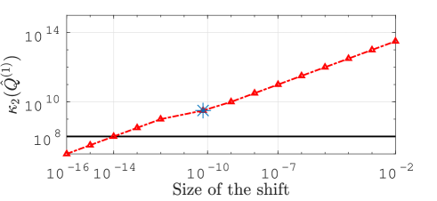
Figure 3: $\kappa_{2}(\hat{Q}^{(1)})$ for test matrix with $\kappa_{2}(X)=10^{15}$, $m=1000$, $n=50$, varying the shift of shiftedCholeskyQR.

6.2 Orthogonality and residual

Next we examine the numerical stability of shiftedCholeskyQR3 (shown in the figures as sCholQR3) and compare it with other popular QR decomposition algorithms, namely, Householder QR, classical and modified Gram-Schmidt (CGS and MGS; we also run them twice, CGS2 and MGS2). We first take $B=I$ and vary $\kappa_{2}(X)$, $m$ and $n$ and investigate the dependence of the orthogonality and residual on them. We set $X$ as in (161). We examine the orthogonality and residual measured by the Frobenius norm under various conditions in Figures 4 through 6. Figure 4 shows the orthogonality $\|\hat{Q}^{T}\hat{Q}-I\|_{F}$ and residual $\|\hat{Q}\hat{R}-X\|_{F}$, where we take $m=300$, $n=10$ and $\kappa_{2}(X)$ was varied from $10^{8}$ to $10^{15}$. In Figure 5, $\kappa_{2}(X)=10^{12}$, $n=50$ and $m$ was varied from 1000 to 10000. In Figure 6, $\kappa_{2}(X)=10^{12}$, $m=1000$ and $n$ was varied from 10 to 500.

We see in Figure 4 that with shiftedCholeskyQR, the orthogonality and the residual are independent of $\kappa_{2}(X)$ and are of $O({\bf u})$, as long as $\kappa_{2}(X)$ is at most $O({\bf u}^{-{1}})$. This is in good agreement with Theorem 4.1. Figures 5 and 6 indicate that the orthogonality and residual increase only mildly with $m$ and $n$. Although they are inevitably overestimates, these also reflect our results (71) and (72). Compared with Householder QR, we observe that shiftedCholeskyQR3 usually produces slightly better orthogonality and residual. With MGS, the deviation from orthogonality increases proportionally to $\kappa_{2}(X)$. As is well known, Gram-Schmidt type algorithms perform well when repeated twice, and we can verify this here. As mentioned in Section 4, an advantage of shiftedCholeskyQR3 is that it is rich in BLAS-3 operations and easily parallelized (it ran more than ten times faster than Gram-Schmidt algorithms in the experiments here). Overall, we see that shiftedCholeskyQR3 is an efficient and reliable method for matrices with condition number at most $O({\bf u}^{-1})$.

Next, we again take $B\neq I$ and test Algorithm 5, comparing it with the stability of other popular QR decomposition algorithms, namely, MGS, CGS2 and MGS2. We varied $\kappa_{2}(B)$, $m$ and $n$ and investigated the orthogonality $\|\hat{Q}^{T}B\hat{Q}-I\|_{F}$ and residual $\|\hat{Q}\hat{R}-X\|_{F}$. Figure 7 shows the results for the case $m=500$, $n=20$, $\kappa_{2}(B)=10^{10}$ and $\kappa_{2}(B)$ was varied from $10^{1}$ to $10^{10}$. Figure 8 takes $m=300$, $n=50$, $\kappa_{2}(X)=10^{10}$ and $\kappa_{2}(B)$ was varied from $10^{8}$ to $10^{15}$. In Figure 9 we took $\kappa_{2}(X)=10^{8}$, $\kappa_{2}(B)=10^{10}$, $n=50$ and $m$ was varied from 500 to 2000. Figure 10 takes $\kappa_{2}(X)=10^{8}$, $\kappa_{2}(B)=10^{10}$, $m=1000$ and $n$ was varied from 50 to 500.

From Figure 7 we see that the orthogonality and residual of shiftedCholeskyQR3 are independent of $\kappa_{2}(X)$ and are of $O({\bf u})$, as long as $\frac{\|X\|_{2}\sqrt{\|B\|_{2}}}{\sqrt{\sigma_{n}(X^{\top}BX)}}\lesssim O({\bf u}^{-{1}})$, reflecting Theorem 5.7. Figure 8 shows that the orthogonality increase rather mildly with $\kappa_{2}(B)$, indicating the dependence on $\kappa_{2}(B)$ suggested by 149 is perhaps improvable; we leave this for future work. Figures 9 and 10 illustrate the orthogonality and residual increase with $m$ and $n$, again mildly. These are also in agreement with (149) and (150) in Theorem 5.7; again, its $m,n$-dependence may be improvable. Compared with CGS2 and MGS2, the orthogonality and residual of CGS2 and MGS2 and that of shiftedCholeskyQR3 are of the same magnitude. Again, shiftedCholeskyQR3 has the advantage of being parallelization-friendly. All our experiments corroborate that shiftedCholeskyQR3 is a reliable method whether $B=I$ or $B\neq I$, for matrices with $\frac{\|X\|_{2}\sqrt{\|B\|_{2}}}{\sqrt{\sigma_{n}(X^{\top}BX)}}<O({\bf u}^{-{1}})$.

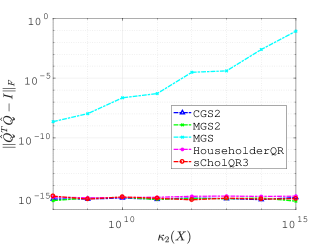
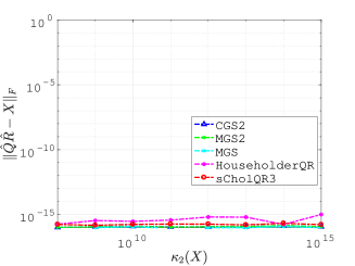
Figure 4: Orthogonality $\|\hat{Q}^{\top}\hat{Q}-I\|_{F}$ and residual $\|\hat{Q}\hat{R}-X\|_{F}$ for test matrices with $m=300$, $n=10$, varying $\kappa_{2}(X)$.

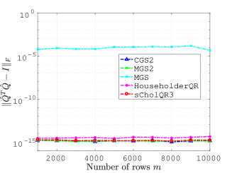
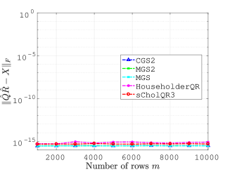
Figure 5: Orthogonality $\|\hat{Q}^{\top}\hat{Q}-I\|_{F}$ and residual $\|\hat{Q}\hat{R}-X\|_{F}$ for test matrices with $\kappa_{2}(X)=10^{12}$, $n=50$, varying $m$.

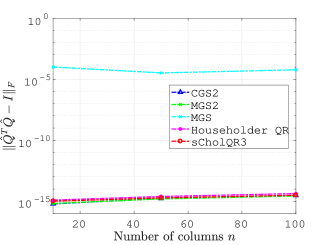
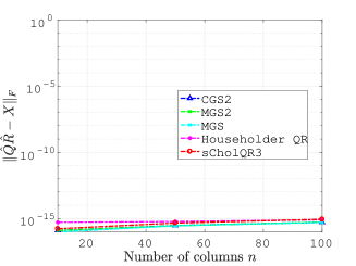
Figure 6: Orthogonality $\|\hat{Q}^{\top}\hat{Q}-I\|_{F}$ and residual $\|\hat{Q}\hat{R}-X\|_{F}$ for test matrices with $\kappa_{2}(X)=10^{12}$, $m=1000$, varying $n$.

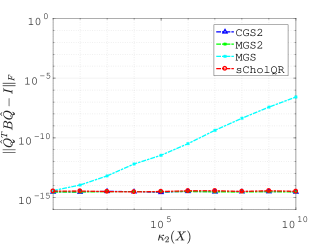
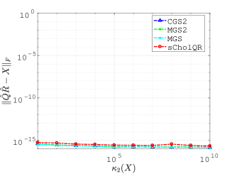
Figure 7: Orthogonality $\|\hat{Q}^{\top}B\hat{Q}-I\|_{F}$ and Residual $\|\hat{Q}\hat{R}-X\|_{F}$ for test matrices with $m=500$, $n=20$, $\kappa_{2}(B)=10^{10}$, varying $\kappa_{2}(X)$.

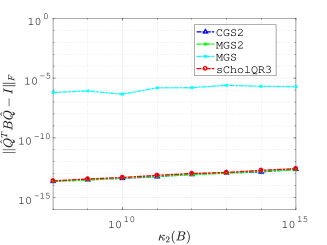
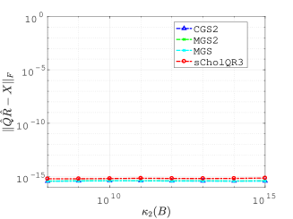
Figure 8: Orthogonality $\|\hat{Q}^{\top}B\hat{Q}-I\|_{F}$ and Residual $\|\hat{Q}\hat{R}-X\|_{F}$ for test matrices with $m=300$, $n=50$, $\kappa_{2}(X)=10^{10}$, varying $\kappa_{2}(B)$.

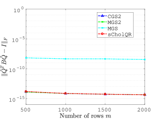
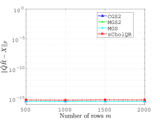
Figure 9: Orthogonality $\|\hat{Q}^{\top}B\hat{Q}-I\|_{F}$ and Residual $\|\hat{Q}\hat{R}-X\|_{F}$ for test matrices with $\kappa(X)=10^{8}$, $\kappa_{2}(B)=10^{10}$, $n=50$, varying $m$.

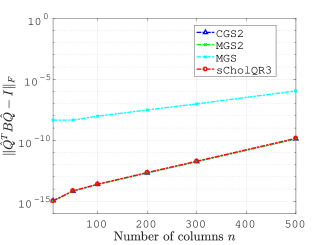
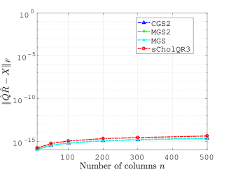
Figure 10: Orthogonality $\|\hat{Q}^{\top}B\hat{Q}-I\|_{F}$ and Residual $\|\hat{Q}\hat{R}-X\|_{F}$ for test matrices with $\kappa_{2}(X)=10^{8}$, $\kappa_{2}(B)=10^{10}$, $m=1000$, varying $n$.

7 Runtime Performance

We next evaluate the runtime performance of shiftedCholeskyQR3 in multi-core CPU environments for both the standard and the oblique case involving a sparse symmetric, positive definite matrix.

7.1 Standard inner product

We used a compute node of the Laurel 2 supercomputer system installed at the Academic Center for Computing and Media Studies, Kyoto University, whose specifications are listed in Table 4. Here we focus on the standard $B=I$ case, to facilitate comparison with available algorithms. Test matrices are generated as in the previous experiments, using (161). Here, random orthogonal matrices are obtained by applying the LAPACK Householder QR routines (dgeqrf and dorgqr) to a random matrix. The code is written in Fortran90 and uses LAPACK and BLAS routines.

Table 5 presents the computational time of several methods, where the QR factorization of matrices whose condition number is $10^{11}$ is computed. Here, we compare shiftedCholeskyQR3 (dgemm and dsyrk versions), Householder QR, and CGS2 (including its blocked version). It is worth noting that dgeqr is a novel LAPACK routine that appropriately uses the TSQR algorithm. The block width in Block CGS2 was empirically tuned. Table 5 clearly shows that shiftedCholeskyQR3 (both dgemm and dsyrk versions) outperforms other methods for all cases. Among methods besides shiftedCholeskyQR3, dgeqr is fastest, probably due to employing TSQR, but shiftedCholeskyQR3 (dsyrk) is more than $1.7$ times faster in every case. These results also indicate that, even if four iterations is required for ill-conditioned problems, iterated CholeskyQR (shown in Algorithm 2) would still be faster than other methods.

It is of interest to compare shiftedCholeskyQR3 with mixedCholQR [18] from the viewpoint of computational time, but implementing and highly tuning double-double gemm or syrk routines (whose input matrices are in double precision) is generally difficult and requires significant effort. We thus estimate the computational cost of mixedCholQR routine; we only discuss the case where gemm is used, but almost the same discussion is applicable when we use syrk. Table 6 presents the results of the benchmark for dgemm, which computes $X^{\top}X$, where $X$ is an $m\times n$ matrix. From this table, we can assume that $700$ GFLOPS is a rough upper bound of the achieved performance. According to the paper on mixed precision CholeskyQR [18], the number of double precision operations required in ddgemm (a double-double precision gemm routine) is $8$ times (Cray-style) or $12.5$ times (IEEE-style) that required in dgemm. Therefore, assuming that double precision operations in ddgemm are performed at $700$ GFLOPS, we can estimate the time (sec.) of ddgemm as $\frac{8\cdot 2}{7}\cdot mn^{2}\cdot 10^{-11}$ (Cray-style) or $\frac{12.5\cdot 2}{7}\cdot mn^{2}\cdot 10^{-11}$ (IEEE-style).

Based on the above estimation and the breakdown of timing results of shiftedCholeskyQR3, we compare shiftedCholeskyQR3 and mixed precision CholeskyQR in Table 7. Here, we ignore the increasing cost for ddpotrf because it is small relative to the total time. From the table, we can expect that shiftedCholeskyQR3 is faster than mixed precision CholeskyQR in this computational environment. Considering this estimation and the fact that a well-tuned ddgemm is currently rarely available, shiftedCholeskyQR3 seems to be more practical than mixed precision CholeskyQR.

Finally we briefly mention the performance of shiftedCholeskyQR3 on large-scale distributed parallel systems. Based on our previous performance evaluation of CholeskyQR2 on the K computer (for details, see [4]), we give a rough estimation of the computational time of shiftedCholeskyQR3 in Table 8, where we estimate the computational time of shiftedCholeskyQR3 as $1.5$ times that of CholeskyQR2, simply based on the number of iterations. From this table, shiftedCholeskyQR3 is expected to be still significantly faster than Householder QR methods (both TSQR and ScaLAPACK routines) in large-scale parallel computation for matrices $\kappa_{2}(X)<{\bf u}^{-1}$.

Table 4: Specifications of the Laurel 2 system.

Item	Specification
CPU	Intel Xeon E5-2695 v4 (Broadwell, 2.1 GHz, 18 cores)
Number of CPUs / node	2
Memory size / node	128 GB
Peak FLOPS / node	1.21 TFLOPS (in double precision)
Compiler	Intel ifort ver. 17.0.6
Compile options	-mcmodel=medium, -shared-intel, -qopenmp
	-O3, -ipo, -xHost
BLAS, LAPACK	Intel MKL ver. 2017.0.6 (-mkl=parallel)

Table 5: Computational time on Laurel 2: $\kappa_{2}(X)=10^{11}$, $m=100,000$ and the number of threads is $36$.

	Time (sec.)
Method	$n=32$	$n=64$	$n=128$	$n=256$
sCholQR3 (dgemm ver.)	$2.62\times 10^{-3}$	$9.16\times 10^{-3}$	$3.32\times 10^{-2}$	$1.16\times 10^{-1}$
sCholQR3 (dsyrk ver.)	$2.39\times 10^{-3}$	$7.44\times 10^{-3}$	$2.45\times 10^{-2}$	$8.20\times 10^{-2}$
dgeqrf $+$ dorgqr	$6.31\times 10^{-2}$	$8.94\times 10^{-2}$	$1.19\times 10^{-1}$	$1.96\times 10^{-1}$
dgeqr $+$ dgemqr	$4.39\times 10^{-3}$	$1.30\times 10^{-2}$	$4.39\times 10^{-2}$	$1.68\times 10^{-1}$
CGS2	$9.60\times 10^{-3}$	$2.31\times 10^{-2}$	$1.40\times 10^{-1}$	$1.24$
Block CGS2	$9.62\times 10^{-3}$	$2.49\times 10^{-2}$	$7.88\times 10^{-2}$	$2.05\times 10^{-1}$

Table 6: Achieved performance of dgemm: $m=100,000$ and the number of threads is $36$.

$n$	$32$	$64$	$128$	$256$	$512$	$1,024$	$4,096$	$16,384$
GFLOPS	$476$	$559$	$539$	$589$	$600$	$624$	$654$	$628$

Table 7: Comparison of shiftedCholeskyQR3 with Mixed Precision CholeskyQR based on the performance estimation for ddgemm: $m=100,000$ and $n=64$.

	shiftedCholeskyQR3		Mixed Precision CholeskyQR
				Cray-style	IEEE-style
	Routine	Time (sec.)	Routine	Time (sec.)	Time (sec.)
sCholQR	dgemm	$1.90\times 10^{-3}$	–	–	–
	dpotrf	$3.00\times 10^{-5}$	–	–	–
	dtrsm	$1.11\times 10^{-3}$	–	–	–
CholQR	dgemm	$1.68\times 10^{-3}$	ddgemm	$\geq 9.36\times 10^{-3}$	$\geq 1.46\times 10^{-2}$
	dpotrf	$2.91\times 10^{-5}$	ddpotrf	$\geq 2.91\times 10^{-5}$	$\geq 2.91\times 10^{-5}$
	dtrsm	$1.31\times 10^{-3}$	dtrsm	$1.31\times 10^{-3}$	$1.31\times 10^{-3}$
	dtrmm	$3.10\times 10^{-5}$	–	–	–
CholQR	dgemm	$1.81\times 10^{-3}$	dgemm	$1.81\times 10^{-3}$	$1.81\times 10^{-3}$
	dpotrf	$3.79\times 10^{-5}$	dpotrf	$3.79\times 10^{-5}$	$3.79\times 10^{-5}$
	dtrsm	$1.24\times 10^{-3}$	dtrsm	$1.24\times 10^{-3}$	$1.24\times 10^{-3}$
	dtrmm	$2.91\times 10^{-5}$	dtrmm	$2.91\times 10^{-5}$	$2.91\times 10^{-5}$
Misc.		$1.36\times 10^{-4}$		$\geq 0$	$\geq 0$
Total		$9.34\times 10^{-3}$		$\geq 1.38\times 10^{-2}$	$\geq 1.91\times 10^{-2}$

Table 8: Estimation of the computational time of shiftedCholeskyQR3 on the K computer: the number of nodes ($=$ MPI processes) is $16,384$.

		Time (sec.)
		Measured			Estimated
$m$	$n$	TSQR	pdgeqrf $+$ pdorgqr	CholQR2	sCholQR3
4,194,304	16	$1.64\times 10^{-3}$	$1.04\times 10^{-2}$	$8.02\times 10^{-4}$	$1.20\times 10^{-3}$
	64	$7.42\times 10^{-3}$	$4.14\times 10^{-2}$	$2.52\times 10^{-3}$	$3.79\times 10^{-3}$
	256	$2.32\times 10^{-1}$	$1.84\times 10^{-1}$	$3.05\times 10^{-2}$	$4.57\times 10^{-2}$
16,777,216	16	$1.84\times 10^{-3}$	$1.13\times 10^{-2}$	$9.06\times 10^{-4}$	$1.36\times 10^{-3}$
	64	$8.82\times 10^{-3}$	$5.65\times 10^{-2}$	$3.13\times 10^{-3}$	$4.70\times 10^{-3}$
	256	$2.40\times 10^{-1}$	$3.92\times 10^{-1}$	$3.38\times 10^{-2}$	$5.07\times 10^{-2}$

7.2 Oblique inner product

In the case of the inner product defined by a positive definite matrix $B$, we focus on large-sparse $B$, as arises commonly in applications. Owing to the sparsity of $B$, orthogonalizing $X$ such that $X^{T}BX=I$ depends heavily on the performance of sparse matrix-vector multiplication (SpMV). Both CGS2 and shiftedCholeskyQR3 would therefore achieve only a fraction of the machine’s peak performance compared with the case when $B$ is dense, where performance would be dictated by dgemm. Optimizing the performance of shiftedCholeskyQR3 for a sparse $B$ involves extracting performance from the computation of the inner product $X^{T}BX$, which in turn depends on

• sparse matrix multiple-vector multiplication kernels [8], and

• the choice of whether $X^{T}BX$ is computed by forming $Y:=BX$ explicitly followed by computing $X^{T}Y$ or in blocks.

By blocking we refer to forming the matrix $Y_{j}:=BX(:,jk:(j+1)k)$ for some block size $k\in[1,n]$ and $j\in(1,n/k)$ in succession, and subsequently calculating the matrix $X^{T}Y_{j}$. The choice of strategy is highly sensitive to both the sparsity structure of $B$, and the cache hierarchy of the architecture on which we execute. For an unbounded cache size, computing $Y$ explicitly will be the fastest strategy since the subsequent operation $Y^{T}X$ has excellent computational intensity. Realistically however, for a small L1 cache or indeed a large $B$, forming $Y$ will cause the entries of $X$ to be evicted from cache, leading to unnecessary cache misses and a slower performance. For a more detailed discussion and performance analysis of the different strategies, we refer the reader to [9, sec. 6.4]; in this section we present the overall speed-up obtained over CGS2 implementations.

Our experiments for a sparse $B$ were carried out on a shared memory system with Intel Xeon E5-2670 (Sandy Bridge) symmetric multiprocessors. There are 2 processors with 8 cores per processor, each with 2 hyperthreads that share a large 20 MB L3 cache. Each core also has access to 32 KB of L1 cache and 256 KB of L2 cache and runs at 2.6 GHz. They support the AVX instruction set with 256-bit wide SIMD registers, resulting in 10.4 GFlop/s of double precision performance per core or 83.2 GFlop/s per processor and a dgemm performance of 59 GFlop/sec. The implementation was parallelized using OpenMP, and compiled using Intel C++ Compiler version 14.0 with -O3 optimization level, with autovectorization turned on for both CPU. Tests are run by scheduling all threads on a single processor with 16 threads with OpenMP ‘compact’ thread affinity, which is set using KMP_SET_AFFINITY.

We use as test problems symmetric positive definite matrices from the University of Florida [1] collection, as listed in Table 9. The matrices are stored and operated upon $B$ using the Compressed Sparse Row (CSR) format and we avoid changing the format to favour performance although the results in [8] strongly suggest that this is beneficial. The reason for this is that oblique QR factorization is usually part of a “larger” program, for example, a sparse generalized eigensolver [9, chap. 4], and hence the storage format needs may be governed by other operations in the parent algorithm, for example, a sparse direct solution, and such software may not exist for the new format. Changing the sparse matrix format to accelerate the factorization may also slow down other parts of the calling program that are not optimized to work with a different format.

Table 9: Test matrices used for benchmarking chol_borth.

Name	Application	Size	Nonzeros	Nonzeros/row
apache2	finite difference	715,176	2,766,523	3.86
bairport	finite element	67,537	774,378	11.46
bone010	model reduction	986,703	47,851,783	48.50
G3_circuit	circuit simulation	1,585,478	7,660,826	4.83
Geo_1438	finite element	1,437,960	60,236,322	41.89
parabolic_fem	CFD	525,825	2,100,225	3.99
serena	finite element	1,391,349	64,131,971	46.09
shipsec8	finite element	114,919	3,303,553	28.74
watercube	finite element	68,598	1,439,940	20.99

We present the performance of shiftedCholeskyQR3 on CPU by varying $n$, i.e., the size of $X$ and compare the results with those from CGS2 in Figure 11. On the CPU, shiftedCholeskyQR3 was faster than CGS2 by a minimum of 3.7 times for $n=16$ and a maximum of 40 times for $n=256$ vectors. The large speedup obtained is only a reflection of the reliance of CGS2 on matrix-vector products, which in the case of sparse matrices, has a particularly poor CPU utilization.

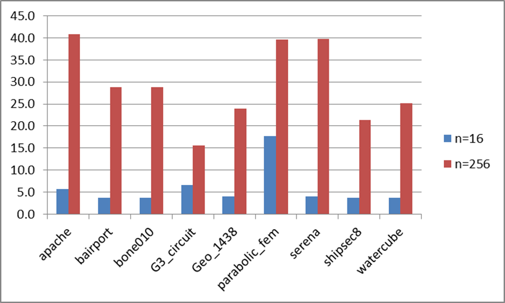
Figure 11: Performance speed-ups of shiftedCholeskyQR3 over CGS2 for sparse problems for varying sizes of $X$.

8 Conclusion and discussion

Our algorithm shiftedCholeskyQR3 combines speed, stability, and versatility (applicable to $B\neq I$). We believe it offers an attractive alternative in high-performance computing to the conventional Householder-based QR factorziation algorithms when $B=I$, and can be the clear algorithm of choice when $B\neq I$.

shiftedCholeskyQR3 as presented could benefit from further tuning, and this work suggests a few future directions. First, the choice of shift $s$ introduced in this paper is conservative, and severely so when $m,n$ are large. Our experiments suggest that a much smaller shift, such as $s=O({\bf u}\|A\|_{2})$, is usually sufficient to avoid breakdown in $\mbox{chol}(A+sI)$, and as illustrated in Figure 3, a smaller shift results in improved conditioning, and hence smaller number of shiftedCholeskyQR iterations. Introduction of a shift strategy that is both stable and efficient is an important remaining task.

Our performance results hold promise for the competitiveness of shiftedCholeskyQR3, and further work will focus on comparing it with other state-of-the-art implementations for QR factorziations such as TSQR in an HPC setting. In the case where $B\neq I$ for a sparse $B$, the performance benefits over CGS2 are remarkable and our algorithm is the clear choice for applications.

Finally, for rank-deficient matrices, shiftedCholeskyQR3 is inapplicable, because $AR$ is rank-deficient for any $R$. This issue is not present in Householder-type methods, and a workaround for shiftedCholeskyQR3 is much desired.

Appendix A A sharper bound on the residual of CholeskyQR2

In [16], the residual of CholeskyQR2 is bounded by $\|\hat{Z}\hat{U}-X\|_{F}\leq 5n^{2}\sqrt{n}{\bf u}\|X\|_{2}$. In this appendix, we derive a sharper bound $5n^{2}{\bf u}\|X\|_{2}$.

In the CholeskyQR2 algorithm in floating-point arithmetic, the QR decomposition $X=ZU$ is computed as follows.

(162) $$\hat{A}=fl(X^{\top}X),\quad\hat{R}=fl({\rm chol}(\hat{A})),\quad\hat{Y}=fl(X\hat{R}^{-1}),$$

(163) $$\hat{C}=fl(\hat{Y}^{\top}\hat{Y}),\quad\hat{S}=fl({\rm chol}(\hat{C})),\quad\hat{Z}=fl(\hat{Y}\hat{S}^{-1}),\quad\hat{U}=fl(\hat{S}\hat{R}).$$

Let us denote the residuals in the first and the second step by $\Delta X$ and $\Delta Y$, respectively, and the forward error in the computation of $\hat{U}$ by $\Delta U$. Then,

(164) $$X+\Delta X = \hat{Y}\hat{R},$$

(165) $$\hat{Y}+\Delta\hat{Y} = \hat{Z}\hat{S},$$

(166) $$\hat{U} = \hat{S}\hat{R}+\Delta U.$$

Using these quantities, the residual of CholeskyQR2 can be evaluated as

(167) $$\|\hat{Z}\hat{U}-X\|_{F} = \|\hat{Z}(\hat{S}\hat{R}+\Delta U)-\hat{Y}\hat{R}+\Delta X\|_{F}$$

$$= \|\Delta\hat{Y}\hat{R}+\hat{Z}\Delta U+\Delta X\|_{F}$$

$$\leq \|\Delta\hat{Y}\|_{F}\|\hat{R}\|_{2}+\|\hat{Z}\|_{2}\|\Delta U\|_{F}+\|\Delta X\|_{F}.$$

In [16] the residual was bounded row-wise, then summed to bound $\|\hat{Z}\hat{U}-X\|_{F}$. The analysis below improves the bound by a factor $\sqrt{n}$ by directly bounding the matrix norm and using the refined analysis employed in Section 3. Now we bound each term in (167). In [16], $\|\hat{R}\|_{2}$ and $\|\Delta U\|_{F}$ (which is denoted as $\|E_{5}\|_{F}$ in [16]) are evaluated as

(168) $$\|\hat{R}\|_{2} \leq 1.1\|X\|_{2},$$

(169) $$\|\Delta U\|_{F} \leq 1.2n^{2}{\bf u}\|X\|_{2}.$$

$\|\hat{Z}\|_{2}$ can be bounded as in Eq. (80) of this paper. To bound $\|\Delta X\|_{F}$, we recall that the $i$th row of $\hat{Y}$, which we denote by $\hat{\bf y}_{i}^{\top}$, is computed from the $i$th row of $X$, which we denote by ${\bf x}_{i}^{\top}$, by triangular solution and therefore it holds that

(170) $$\hat{\bf y}_{i}^{\top}={\bf x}_{i}^{\top}(\hat{R}+\Delta\hat{R}_{i})^{-1}\quad(i=1,2,\ldots,m),$$

where $\Delta\hat{R}_{i}$ is the backward error of the triangular solution. According to [16], $\|\Delta\hat{R}_{i}\|_{2}$ is bounded as

(171) $$\|\Delta\hat{R}_{i}\|_{2}\leq 1.2n\sqrt{n}{\bf u}\|X\|_{2}.$$

Hence, by denoting the $i$th row of $\Delta X$ by $\Delta{\bf x}_{i}^{\top}$ and noting the relationship $\Delta{\bf x}_{i}^{\top}=-\hat{\bf y}_{i}^{\top}\Delta\hat{R}_{i}$, we obtain

(172) $$\|\Delta X\|_{F}=\sqrt{\sum_{i=1}^{m}\|\hat{\bf y}_{i}^{\top}\Delta\hat{R}_{i}\|^{2}}=\sqrt{\sum_{i=1}^{m}\|\hat{\bf y}_{i}^{\top}\|^{2}}\max_{1\leq i\leq m}\|\Delta\hat{R}_{i}\|_{2}\leq\|\hat{Y}\|_{F}\cdot 1.2n\sqrt{n}{\bf u}\|X\|_{2}.$$

Since the singular values of $\hat{Y}$ are bounded by $\frac{\sqrt{69}}{8}$ (see the proof of Corollary 3.2 in [16]), $\|\hat{Y}\|_{F}\leq\sqrt{n}\|\hat{Y}\|_{2}\leq\frac{\sqrt{69}}{8}\sqrt{n}$. Inserting this into (172), we have

(173) $$\|\Delta X\|_{F}\leq 1.3n^{2}{\bf u}\|X\|_{2}.$$

A bound on $\|\Delta Y\|_{F}$ can be obtained by replacing $X$ and $\hat{Y}$ in (172) with $\hat{Y}$ and $\hat{Z}$, respectively, and noting that $\|\hat{Y}\|_{2}\leq\frac{\sqrt{69}}{8}$ and $\|\hat{Z}\|_{F}\leq\sqrt{n}\sqrt{1+6(mn{\bf u}+n(n+1){\bf u})}\leq 1.1\sqrt{n}$ (see Theorem 3.3 in [16]). The result is

(174) $$\|\Delta\hat{Y}\|_{F}\leq 1.4n^{2}{\bf u}.$$

Putting all these together and inserting into (167), we finally have

(175) $$\|\hat{Z}\hat{U}-X\|_{F} \leq 1.4n^{2}{\bf u}\cdot 1.1\|X\|_{2}+\frac{\sqrt{76}}{8}\cdot 1.2n^{2}{\bf u}\|X\|_{2}+1.3n^{2}{\bf u}\|X\|_{2}$$

$$\leq 5n^{2}{\bf u}\|X\|_{2}.$$

References

- [1] T. A. Davis and Y. Hu, The University of Florida Sparse Matrix Collection, ACM Trans. Math. Softw., 38 (2011), pp. 1:1–1:25, https://doi.org/10.1145/2049662.2049663, http://doi.acm.org/10.1145/2049662.2049663.
- [2] J. Demmel, On floating point errors in Cholesky, Tech. Report 14, LAPACK Working Note, 1989.
- [3] J. Demmel, L. Grigori, and M. Hoemmen, Implementing communication-optimal parallel and sequential QR factorizations, arXiv:0809.2407, (2008).
- [4] T. Fukaya, Y. Nakatsukasa, Y. Yanagisawa, and Y. Yamamoto, CholeskyQR2: a simple and communication-avoiding algorithm for computing a tall-skinny QR factorization on a large-scale parallel system, in Proceedings of the 5th Workshop on Latest Advances in Scalable Algorithms for Large-Scale Systems, IEEE Press, 2014, pp. 31–38.
- [5] L. Giraud, J. Langou, M. Rozložník, and J. Eshof, Rounding error analysis of the classical gram-schmidt orthogonalization process, Numer. Math., 101 (2005), pp. 87–100.
- [6] G. H. Golub, V. Loan, and C. F., Matrix Computations, The Johns Hopkins University Press, 4th ed., 2013.
- [7] N. J. Higham, Accuracy and Stability of Numerical Algorithms, SIAM, Philadelphia, PA, USA, second ed., 2002.
- [8] R. Kannan, Efficient sparse matrix multiple-vector multiplication using a bitmapped format, in 20th IEEE International Conference on High Performance Computing (HiPC’13), December 2013, pp. 286–294, https://doi.org/10.1109/HiPC.2013.6799135.
- [9] R. Kannan, Numerical Linear Algebra problems in Structural Analysis, PhD thesis, School of Mathematics, The University of Manchester, 2014.
- [10] B. R. Lowery and J. Langou, Stability analysis of QR factorization in an oblique inner product, arXiv:1401.5171, (2014).
- [11] Multiprecision Computing Toolbox. Advanpix, Tokyo. http://www.advanpix.com.
- [12] M. Rozložník, M. Tŭma, A. Smoktunowicz, and J. Kopal, Numerical stability of orthogonalization methods with a non-standard inner product, BIT, (2012), pp. 1–24.
- [13] S. M. Rump and T. Ogita, Super-fast validated solution of linear systems, J. Comput. Appl. Math., 199 (2007), pp. 199–206.
- [14] A. Stathopoulos and K. Wu, A block orthogonalization procedure with constant synchronization requirements, SIAM J. Sci. Comp, 23 (2002), pp. 2165–2182.
- [15] L. N. Trefethen and D. Bau, Numerical Linear Algebra, SIAM, Philadelphia, 1997.
- [16] Y. Yamamoto, Y. Nakatsukasa, Y. Yanagisawa, and T. Fukaya, Roundoff error analysis of the CholeskyQR2 algorihm, Electron. Trans. Numer. Anal, 44 (2015), pp. 306–326.
- [17] Y. Yamamoto, Y. Nakatsukasa, Y. Yanagisawa, and T. Fukaya, Roundoff error analysis of the CholeskyQR2 algorithm in an oblique inner product, JSIAM Letters, 8 (2016), pp. 5–8.
- [18] I. Yamazaki, S. Tomov, and J. Dongarra, Mixed-precision Cholesky QR factorization and its case studies on Multicore CPU with Multiple GPUs, SIAM J. Sci. Comp, 37 (2015), pp. C307–C330.
- [19] Y. Yanagisawa, T. Ogita, and S. Oishi, A modified algorithm for accurate inverse Cholesky factorization, Nonlinear Theory and Its Applications, IEICE, 5 (2014), pp. 35–46.