A Monocular Vision System for Playing Soccer
in Low Color Information Environments

Abstract

Humanoid soccer robots perceive their environment exclusively through cameras. This paper presents a monocular vision system that was originally developed for use in the RoboCup Humanoid League, but is expected to be transferable to other soccer leagues. Recent changes in the Humanoid League rules resulted in a soccer environment with less color coding than in previous years, which makes perception of the game situation more challenging. The proposed vision system addresses these challenges by using brightness and texture for the detection of the required field features and objects. Our system is robust to changes in lighting conditions, and is designed for real-time use on a humanoid soccer robot. This paper describes the main components of the detection algorithms in use, and presents experimental results from the soccer field, using ROS and the igus^® Humanoid Open Platform as a testbed. The proposed vision system was used successfully at RoboCup 2015.

I Introduction

RoboCupSoccer is an ongoing effort to develop humanoid soccer robots, with the vision of them being able to win against the FIFA world champion team by 2050. Essential to this effort is the ability of the robots to perceive the game situation in real-time under realistic conditions. Each year, the RoboCup soccer leagues update their rules, to force participating teams to develop more advanced features for their robots, and to make the competitions more similar to real soccer games [1]. For the 2015 RoboCup, numerous changes were made in the Humanoid league rules that affect visual perception, including in particular the reduction of color coding on objects on the field. The ball is now only specified to be at least 50% white, and the goal posts are now white instead of yellow. Moreover, the field lines—a major feature for localization on the field—are now painted onto artificial grass, and are as a result no longer white. Due to these changes, the simple color segmentation and blob detection approaches that were quite popular in the past [2] [3] have become unsuitable. This paper presents a monocular vision system that addresses the new challenges by relying more on relative brightness and texture. It was tested at RoboCup 2015 and found to perform well under the new rules.

II Related Work

Visual perception is a much researched topic within the RoboCup community, and many approaches have been developed in the past, albeit now for older versions of the rules.

Strasdat et al. [4], for example, developed a probabilistic method for robot localization relying on many unreliable detections of field features and field lines. Schulz and Behnke [5] demonstrated that the tracking of the robot pose is possible by using field lines only.

Many attempts have been made to reduce the reliance on color classification. For example, Schulz et al. [6] learned to detect the ball by classifying regions of interest with a neural network, based on color contrast and brightness features. Similarly, Metzler et al. [7] learned the detection of Nao robots based on color histograms in regions of interest.

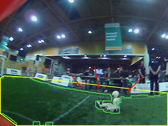
(a) Convex hull of the green regions in the image (yellow), and the unwanted area (red arrows).

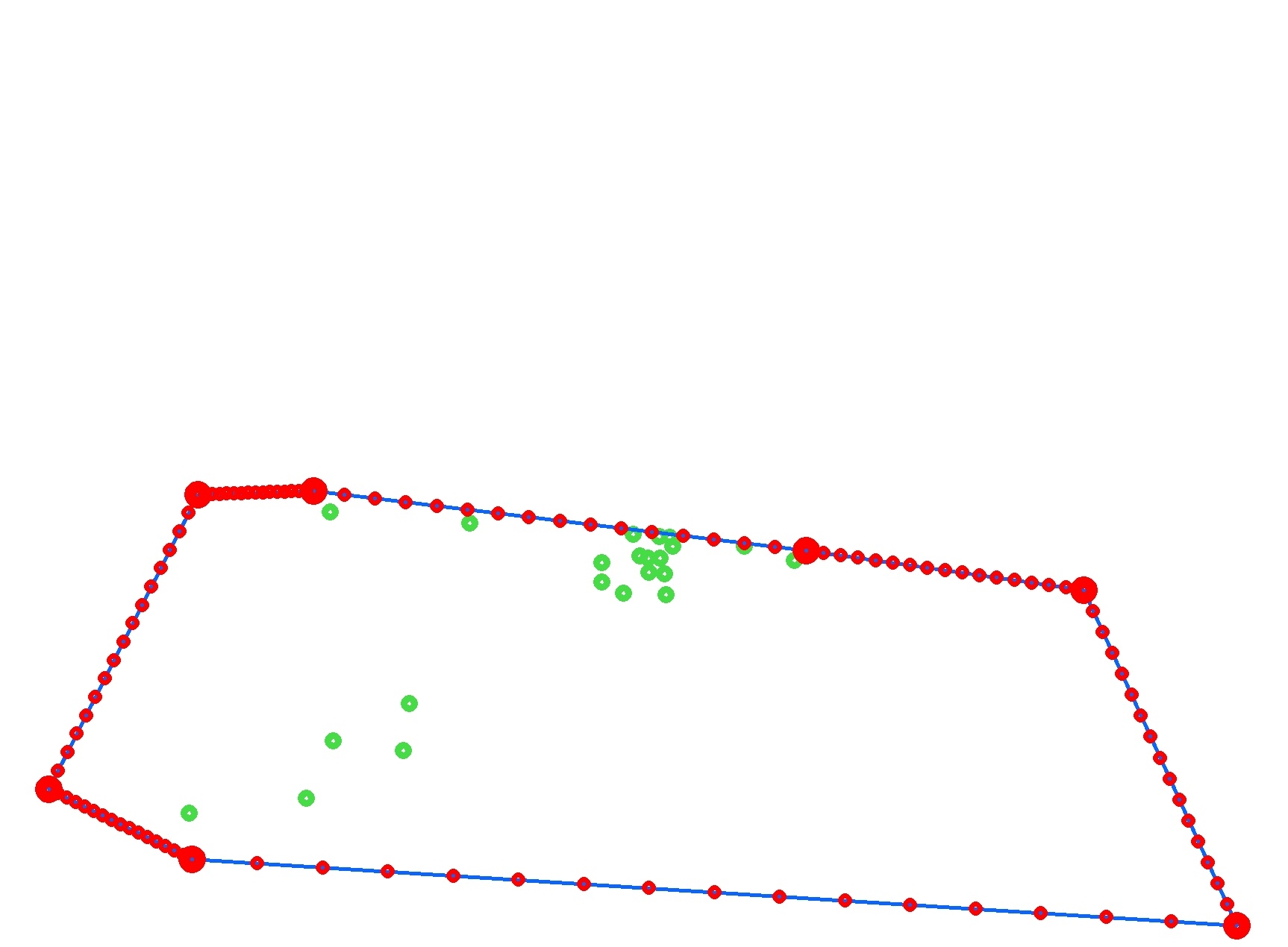
(b) Boundary points of the undistorted convex hull. Green points are vertices of the raw extracted regions.

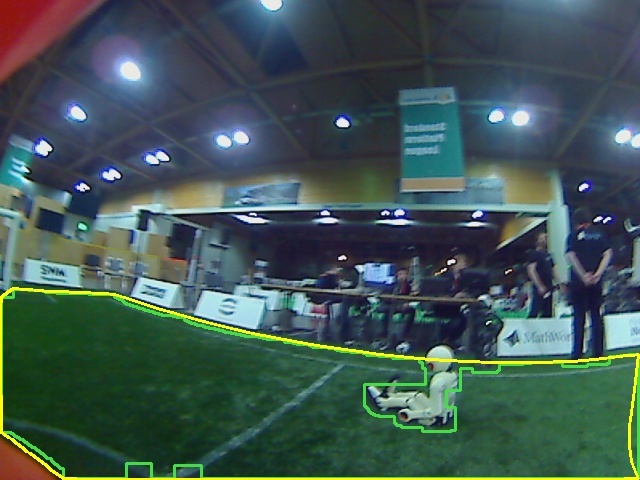
(c) Final detected field area.

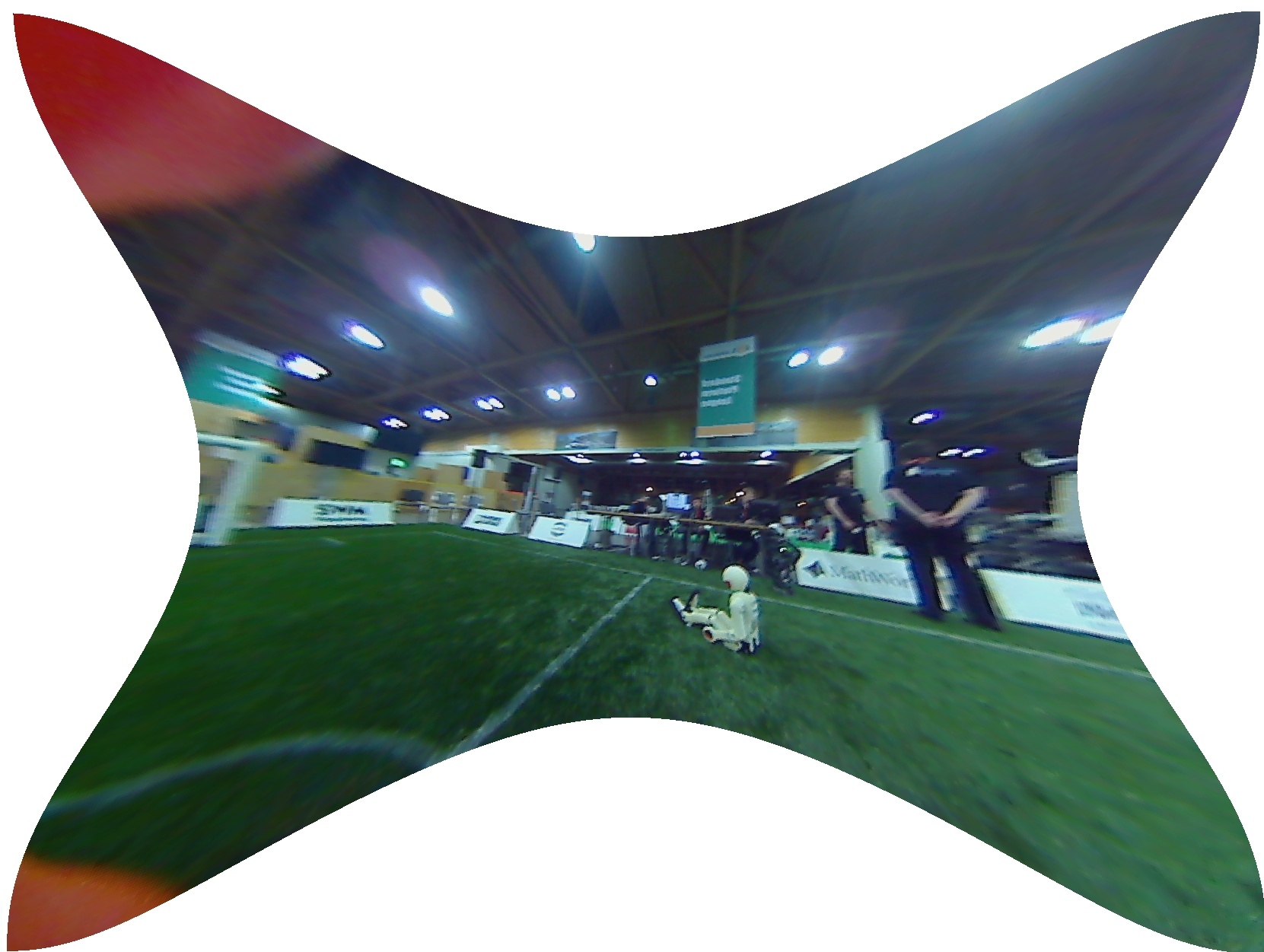
(d) An undistorted captured image.

Figure 1: Stages of field boundary detection.

More recent examples include the work of Houliston et al. [8], who introduced an adaptive lookup table in order to deal with changes in image illumination. Schwarz et al. [9] proposed a calibration-free vision system in the standard platform league (SPL), based on heuristics such as that the field is the maxima of the weighted histograms of each channel in the image. Härtl et al. [10] presented work on color classification based on color similarity. To address the recent changes in goal color in the SPL, Cano et al. [11] proposed a method for detecting white goals based on pixel intensities using the Y channel of the YUV color space. In order to cope with variations in illumination, Reinhardt [12] proposed different heuristics that can be applied to color histograms. The middle size league (MSL) has used white goals for a number of years, but most approaches used in the MSL are not applicable to the humanoid league due to omnivision and active sensors such as Kinects being allowed.

The contributions of this paper include the introduction of several novel algorithms and techniques for performing soccer-related vision detections, and the development of a soccer vision system that can run in real-time and work under various lighting conditions, and in a low color information environment.

III System Overview

In our vision system, the image is captured in the RGB color format, and converted to the HSV (Hue, Saturation and Value) color space using OpenCV conversion routines [13]. For color classification, we use the HSV color space due to its intuitive nature, in particular its ability to separate brightness and chromatic information [14]. To ensure the short term consistency of the colors in the captured images, and to prevent unwanted abrupt image composition changes due to the camera itself, a fixed set of camera parameters, including for example brightness and exposure, are set in the camera device. In some cases, the camera may disconnect and reconnect from the USB bus, such as possibly when the robot falls. For this situation, the camera image acquisition thread is designed in such a way that it can automatically detect a disconnect event and reconnect to the camera device.

The vision process nominally acquires camera images at $30\text{\,}\mathrm{Hz}$. Each captured image is labeled with a timestamp, along with the local robot position and orientation at that time. Feature detection routines are applied to each image, in the order field boundary, ball, lines, circle, goal posts, and finally obstacle. Due to the unwanted overhead of transferring images across process boundaries, all image acquisition and processing routines are implemented in a single ROS node, referred to as the vision module. The vision module publishes its detections and outputs to suitable ROS topics, which can then be used by other nodes.

IV Camera Calibration

In the igus^® Humanoid Open Platform, we use a wide-angle lens to allow more of the environment to be seen at once. This introduces significant distortion, however, which must be compensated when projecting image coordinates into egocentric world coordinates. The OpenCV [13] chessboard calibration procedure is used to determine intrinsic camera parameters that characterize the distortion. The following pinhole camera distortion model, including both radial and tangential distortion components, is used:

$$a =\frac{x}{z},\quad b=\frac{y}{z},\quad r^{2}=a^{2}+b^{2},$$ (1)

$$\hat{x} =a\Bigl{(}\!\tfrac{1+k_{1}r^{2}+k_{2}r^{4}+k_{3}r^{6}}{1+k_{4}r^{2}+k_{5}r^{4}+k_{6}r^{6}}\!\Bigr{)}+2p_{1}ab+p_{2}(r^{2}+2a^{2}),$$ (2)

$$\hat{y} =b\mspace{2.0mu}\Bigl{(}\!\tfrac{1+k_{1}r^{2}+k_{2}r^{4}+k_{3}r^{6}}{1+k_{4}r^{2}+k_{5}r^{4}+k_{6}r^{6}}\!\Bigr{)}+2p_{2}ab+p_{1}(r^{2}+2b^{2}),$$ (3)

$$u =c_{x}+f_{x}\hat{x},\quad v=c_{y}+f_{y}\hat{y},$$ (4)

where $(c_{x},c_{y})$ is the principal point, and $f_{x}$ and $f_{y}$ are the focal lengths, all in pixel units. $k_{1}$ to $k_{6}$ are the radial distortion coefficients, and $p_{1}$ and $p_{2}$ are the tangential distortion coefficients. The input $(x,y,z)$ is a world vector in the camera frame, and the output $(u,v)$ is the corresponding distorted image pixel position. For simplicity, higher-order coefficients and thin prism distortions are not included in the model. Due to limitations of the undistortion functionality in OpenCV, producing poor results especially near the corners, a more accurate and efficient undistortion method was implemented based on the Newton-Raphson method. This method is used to populate a pair of lookup tables that allow $O(1)$ distortion and undistortion operations at runtime. The effect of undistortion is shown in Fig. 1(d).

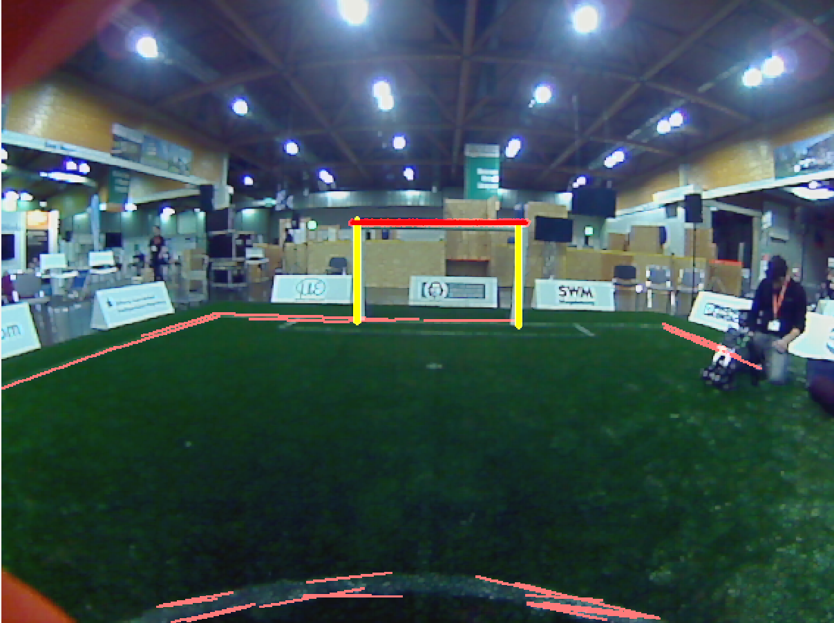
(a) The output of the probabilistic Hough line detection on the extracted edges (thin red lines).

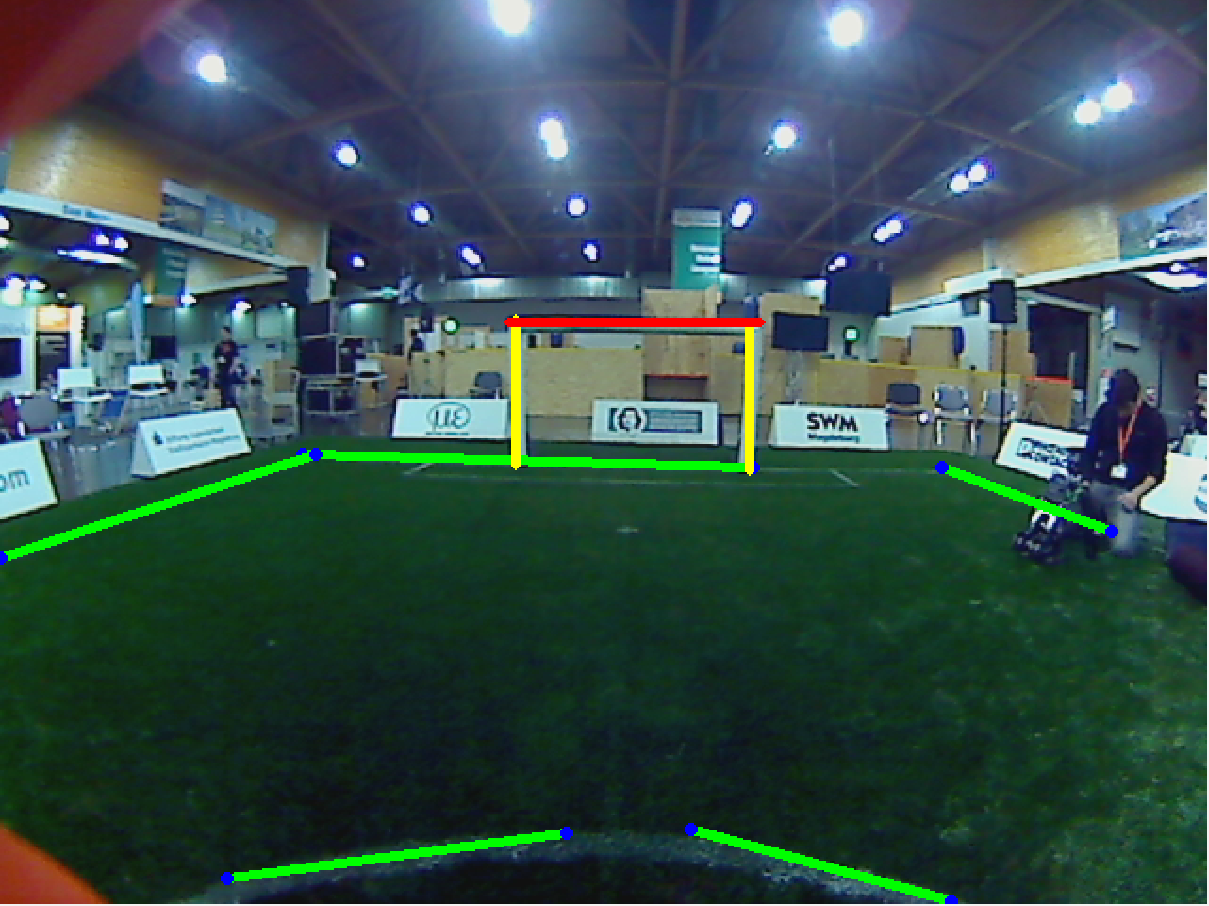
(b) The final field line (green lines) and goal post (yellow lines) detections, marked in the captured image.

Figure 5: Line detections on a soccer field.

The distortion model allows projection to the camera frame, but further extrinsic parameters are required to allow projection to egocentric world coordinates. More specifically, at each point in time the transformation from the egocentric world frame to the camera frame must be known, which is both time- and robot-specific. We use the ROS-native tf2 library [15] for this purpose, which amalgamates joint position and robot kinematics information to produce the required time-varying transforms. Although we have a relatively exact kinematic model of the robot, some variation still occurs in the real hardware, resulting in potentially large projection errors for distant objects. To account for this, we calibrate the kinematics on each robot using a hill-climbing approach that tunes translation and rotation offsets between the torso, which contains the IMU, and the camera. These offsets are crucial for good performance of the pixel-to-egocentric coordinate projection algorithm. The effect of the kinematic calibration is demonstrated in Fig. 2. For reference, the corresponding raw captured image is shown in Fig. 5(b). Note that the calibration procedure is interactive in the sense that the user can select a number of points in the captured image and the corresponding true field locations. This is used as the input to the hill-climbing method, which seeks to minimize the reprojection error of the selected points. This completes the calibration of the camera for the purposes of the vision module.

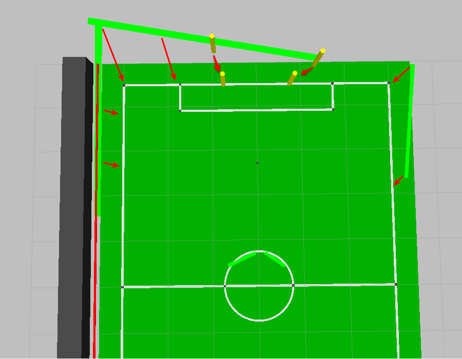
(a) Projected line and goal post detections prior to kinematic calibration, with projection errors marked.

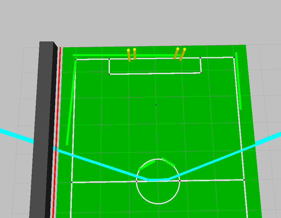
(b) Projected line and goal post detections after kinematic calibration, with the field of view marked.

Figure 2: Effect of the kinematic calibration of the camera.

V Feature Detection Algorithms

V-A Field Detection

The soccer field used in RoboCup competitions is green, so field detection can be based on color segmentation in the HSV color space. Using a user-selected green color range, a binarized image is constructed, and all connected components that appear below the estimated horizon are found. Connected regions that have an area greater than some chosen threshold are taken into consideration for the extraction of a field boundary. If too many separate green regions exist, a set maximum number of regions are considered, prioritized by size and distance from the bottom of the image. Although it is a common approach to find a convex hull of all green areas directly in the image [11] [2], more care needs to be taken in our case due to the significant image distortion. Fig. 1(a) shows how the convex hull may include parts of the image that are not the field. To exclude these unwanted areas, the vertices of the connected regions are first undistorted before calculating the convex hull, shown in Fig. 1(b). The convex hull points and intermediate points on each edge are then distorted back into the raw captured image, and the resulting polygon is taken as the field boundary. An example of the final detected field polygon is shown in Fig. 1(c).

V-B Ball Detection

In previous years, most RoboCup teams used simple color segmentation and blob detection based approaches to find the orange ball. Now that the ball is mostly white, however, and generally with a pattern, such simple approaches no longer work effectively, especially since the lines and goal posts are also white. Our approach is divided into two stages. In the first stage, ball candidates are generated based on color segmentation, color histograms, shape, and size. White connected components in the image are found, and the Ramer-Douglas-Peucker algorithm [16] is applied to reduce the number of polygon vertices in the resulting regions. This is advantageous for quicker subsequent detection of circle shapes. The detected white regions are searched for at least one third full circle shapes within the expected radius ranges using a technique very similar to Algorithm 3. Color histograms of the detected circles are calculated for each of the three HSV channels, and compared to expected ball color histograms using the Bhattacharyya distance [13]. Circles with a suitably similar color distribution to expected are considered to be ball candidates.

Figure 3: Extending one positive sample (leftmost) to ten, by applying rotations and mirroring operations.

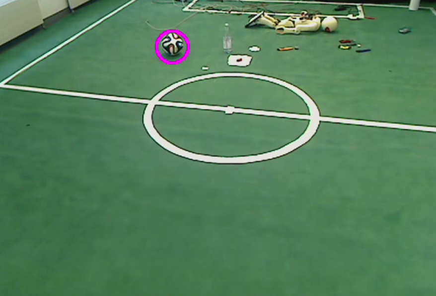
(a) Ball detection in an undistorted image, with other white objects.

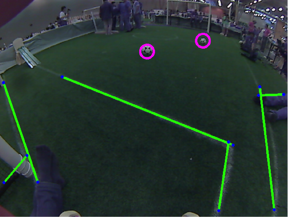
(b) Multiple balls detected on a soccer field, with image distortion.

Figure 4: Ball detections under various conditions.

Algorithm 1 Merge similar line segments.

0:  A set of line segments $S$

0:  A set of line segments $N$ where $\lvert N\rvert\leq\lvert S\rvert$

1:  $N\leftarrow S$

2:  repeat

3:     $M\leftarrow N$

4:     $m\leftarrow\lvert M\rvert$

5:     $N\leftarrow\emptyset$

6:     while $M\neq\emptyset$ do

7:        $X\leftarrow$ Any element of $M$

8:        $M\leftarrow M\setminus\{X\}$

9:        $\hat{m}\leftarrow\lvert M\rvert$

10:        for $Y\in M$ do

11:           if $MinDistance(X,Y)<$0.25\text{\,}\mathrm{m}$$ and $AngleDif\!f(X,Y)<15$^∘ then

12:              $N\leftarrow N\cup\{Merge(X,Y)\}$

13:              $M\leftarrow M\setminus\{Y\}$

14:              break

15:           end if

16:        end for

17:        if $\lvert M\rvert=\hat{m}$ then

18:           $N\leftarrow N\cup\{X\}$

19:        end if

20:     end while

21:  until $\lvert N\rvert=m$

22:  return  $N$

Algorithm 2 $Merge(X,Y)$: Merge two line segments.

0:  Two line segments $X$ and $Y$

0:  Merged line segment $Q$

1:  $\theta\leftarrow 0$

2:  $X_{m}=Midpoint(X)$

3:  $Y_{m}=Midpoint(Y)$

4:  $r\leftarrow\lVert X\rVert/(\lVert X\rVert+\lVert Y\rVert)$

5:  $P\leftarrow rX_{m}+(1-r)Y_{m}$

6:  if $\lVert X\rVert\geq\lVert Y\rVert$ then

7:     $\theta\leftarrow Slope(X)$

8:  else

9:     $\theta\leftarrow Slope(Y)$

10:  end if

11:  $Z\leftarrow$ The line through point $P$ of slope $\theta$

12:  $S\leftarrow$ Orthogonal projections of the endpoints of $X$ and        $Y$ onto $Z$

13:  $Q\leftarrow$ The largest line segment defined by points in $S$

14:  return  $Q$

In the second stage of processing, a dense histogram of oriented gradients (HOG) descriptor [17] is applied in the form of a cascade classifier, with use of the AdaBoost technique. Using this cascade classifier, we reject those candidates that do not have the required set of HOG features. The AdaBoost technique is used because it provides a powerful bound on the generalization performance [18]. In contrast to what is suggested in [17] however, which was targeted at pedestrian detection, we do not use a multi-scale sliding window technique. Instead, to save computational time, we only apply the HOG descriptor to the regions suggested by the ball candidates. The aim of using the HOG descriptor is to find a description of the ball that is largely invariant to changes in illumination and lighting conditions. In contrast to other common feature descriptors, such as SIFT [19], HOG features are easy to visualize [20], and have for example been found to be more reliable than SIFT in pedestrian detection [17]. The HOG descriptor is not rotation invariant however, so to detect the ball from all angles, and to minimize the user’s effort in collecting training examples, each positive image is rotated by ±10^∘ and ±20^∘, selectively mirrored, with the resulting images being presented as new positive samples. Greater rotations are not considered to allow the cascade classifier to learn the shadow under the ball. So in summary, each positive sample that the user provides is extended to a total of 10 positive samples, as shown in Fig. 3. With a set of about 400 positive and 700 negative samples that are gathered directly from the robot camera and with 20 weak classifiers, training takes approximately 10 hours.

As demonstrated in Fig. 4, the described approach can detect balls with very few false positives, even in environments cluttered with white and with varying lighting conditions. In our experiments, we found that this approach can detect the FIFA size 4 ball up to four meters away. An interesting result is that our approach can find the ball in undistorted and distorted images with the same classifier. A full set of generalized Haar wavelet features [21] was tested on the same data set, and although the result was comparable, the training time was about 10 times slower than for the HOG descriptor. A Local Binary Patterns (LBP) feature classifier [22] was implemented in another comparative test, but the ball detection results were poor.

TABLE I: Helper functions used in the algorithms.

$MinDistance(X,Y)$	Returns the minimum distance between two line segments $X$ and $Y$
$AngleDif\!f(X,Y)$	Returns the angle between two line segments in degrees
$Merge(X,Y)$	See Algorithm 2
$Midpoint(X)$	Returns the midpoint of a line segment
$Slope(X)$	Returns the slope of a line segment
$MaxPtDistance(S)$	Returns the maximum distance between any pair of points in the set $S$
$GetBisector(X)$	Returns the perpendicular bisector line of the given line segment
$HasIntersection(X,Y)$	Returns whether two line segments intersect at a point
$GetIntersection(X,Y)$	Returns the intersection point of two line segments
$DistanceToLine(P,X)$	Returns the Euclidean distance between point $P$ and line segment $X$
$Mean(S)$	Returns the mean of the points in the set $S$

V-C Field Line Detection

Due to the introduction of artificial grass in the RoboCup humanoid league, the lines are no longer clearly visible and identifiable on the field. In past years, many teams based their line detection approaches on the segmentation of the color white. This is no longer a robust approach due to the increased number of white objects on the field, and due to the visual variability of the lines. Our approach is to detect spatial changes in brightness in the image using a canny edge detector [23] on the V channel of the HSV color space. The V channel encodes brightness information, and the result of the canny edge detector on this input is quite robust to changes in lighting conditions, so there is no need to tune parameters for changing lighting conditions. A probabilistic Hough line detector [24] is used to extract line segments of a certain minimum size from the detected edges. This helps to reject edges from white objects in the image that are not lines. The output line segments are filtered in the next stage to avoid false positive line detections where possible. A thresholding technique is used to try to ensure that the detected lines cover white pixels in the image, have green pixels on either side, and are close on both sides to edges returned by the edge detector. The last of these checks is motivated by the expectation that white lines, in an ideal scenario, will produce a pair of high responses in the edge detector, one on each border of the line. Ten equally spaced points are chosen on each line segment under review, and two normals to the line are constructed at each of these points, of approximate $5\text{\,}\mathrm{cm}$ length in each of the two directions. The pixels in the captured image underneath these normals are checked for white color and green color, and the output of the canny edge detector is checked for high response. The number of instances where these three checks succeed are independently totaled, and if all three counts—$V_{W}$, $V_{G}$ and $V_{E}$ respectively—exceed the configured thresholds, the line segment is accepted, otherwise the line segment is rejected.

In the final stage, similar line segments are merged with each other, as appropriate, to produce fewer and bigger lines, as well as cover those line segments that might be partially occluded by another robot. Prior to merging, we project each line segment to the egocentric world coordinates. The merging algorithm is detailed in Algorithm 1, which in turn uses Algorithm 2 to perform the individual merge operations. A list of the simple helper functions that are used in the algorithms in this paper is presented in Table I. Note that the constant thresholds used in Algorithm 1, are indicating the maximum allowed difference in angle and distance between two lines to be merged, and the numeric values are suitable for the current humanoid league field dimensions.

The final result is a set of line segments that relates to the lines and center circle on the field. Line segments that are under a certain threshold in length undergo a simple circle detection routine, detailed in Algorithm 3, to find the location of the center circle. In our experiments, we found that this approach can detect circle and line segments up to $4.5\text{\,}\mathrm{m}$ away.

We generate a probability estimation for each line detection, so that a localization algorithm for example can assign higher weights to detections of higher probability. For a detected line $X$ of length $L$, and check counts $V_{G}$ and $V_{E}$, the probability $P(X)$ of the detection is calculated as

$$P(L,V_{G},V_{E})=\begin{cases}\frac{V_{G}}{V_{GM}}\cdot\frac{V_{E}}{V_{EM}}\cdot\frac{L-1}{3}&\text{if $1<L<3$},\\[2.0pt] \frac{V_{G}}{V_{GM}}&\text{if $L\geq 3$},\\[2.0pt] 0&\text{if $L\leq 1$},\end{cases}$$ (5)

where $V_{GM}$ is the maximum possible value of $V_{G}$, and $V_{EM}$ is the maximum possible value of $V_{E}$. For a detected circle $C$, consisting of line segments $X_{i}$ for $i=1\ldots n$, with corresponding check counts $V_{Gi}$ and $V_{Ei}$, the probability $P(C)$ of the detection is calculated as

$$P(C)=\frac{\>\sum\limits_{i=1}^{n}{V_{G}}_{i}\>}{nV_{GM}}\cdot\frac{\>\sum\limits_{i=1}^{n}{V_{E}}_{i}\>}{nV_{EM}}\cdot\frac{MaxPtDistance(P)}{0.75},$$ (6)

where $P$ is the set of estimated circle centre points, as calculated by Algorithm 3.

Algorithm 3 Detect circle from line segments.

0:  A set of line segments $S$

0:  A boolean flag whether a circle is detected

0:  The centre $C\in\mathbb{R}^{2}$ of the detected circle

1:  $P\leftarrow\emptyset$

2:  for all Line segments $X,Y\in S$ such that $X\neq Y$ do

3:     $X_{B}\leftarrow$ $GetBisector(X)$

4:     $Y_{B}\leftarrow$ $GetBisector(Y)$

5:     if $HasIntersection(X_{B},Y_{B})$ then

6:        $C\leftarrow GetIntersection(X_{B},Y_{B})$

7:        if $DistanceToLine(C,X)\approx 0.75$ and $DistanceToLine(C,Y)\approx 0.75$ then

8:           $P\leftarrow P\cup\{C\}$

9:        end if

10:     end if

11:  end for

12:  if $\lvert P\rvert\geq 5$ and $MaxPtDistance(P)<0.75$ then

13:     return  $\textbf{true}{},\,Mean(P)$

14:  end if

15:  return  $\textbf{false}{},\,(0,0)$

*: Note that the number $0.75$ in this algorithm is related to the expected circle radius in metres.

V-D Goal Detection

In our vision module, detection of the white goal posts is divided into two stages. In the first stage, the image is binarized using color segmentation of the color white, defined as a particular region of the HSV color space by the user. A sample output is shown in Fig. 6(a). Horizontal and vertical lines are then extracted from the binarized image using probabilistic Hough line detection [24]. Using a similar approach as for field line detection, the detected vertical and horizontal line segments are merged together to produce fewer, bigger lines. The main idea behind merging is to have one line segment on each goal post, instead of two on each side. Moreover, by merging line segments we can overcome only partially observable goal posts, and motion-blurred images in which the background may blend into some part of the goal post. The result of the merging is shown in Fig. 6(b). In the second stage of goal post detection, each of the vertical line segments that do not meet the following criteria are rejected.

• The length of the line segment must be within a certain range, dependent on the distance from the robot to the projected bottom point of the line.

• The bottom of the line must be within the field.

• The top of the line must be above the estimated horizon.

• On a kid-size field, if the goal post candidate is more than $2\text{\,}\mathrm{m}$ from the robot there must be one horizontal line segment close to the candidate.

To reject the vertical line segments that might belong to a standing white robot, we check the homogeneity of the texture of each of the merged vertical candidates. To do this, we calculate 10 equally spaced points on the line, and search locally around each of these points for large changes in the H channel of the HSV color space. If many changes in the H channel are observed, the candidate is rejected. Experiments have shown that this approach can detect goal posts up to $5\text{\,}\mathrm{m}$ away.

As for field lines, we assign a probability $P(G)$ to detected goal posts, using the equation

$$P(G)=\begin{cases}\tfrac{3}{4}&\text{if $n=1$},\\ 1-\tfrac{1}{6}\bigl{\lvert}D-\lVert X_{1}-X_{2}\rVert\bigr{\rvert}&\text{if $n=2$},\\ 1-\frac{n}{5}&\text{if $3\leq n\leq 4$},\\ 0&\text{if $n\geq 5$},\\ \end{cases}$$ (7)

where $n$ is the number of the detected goal posts, $D$ is the known goal width, and $X_{1},\ldots,X_{n}$ are the egocentric world vectors to the $n$ detected goal posts.

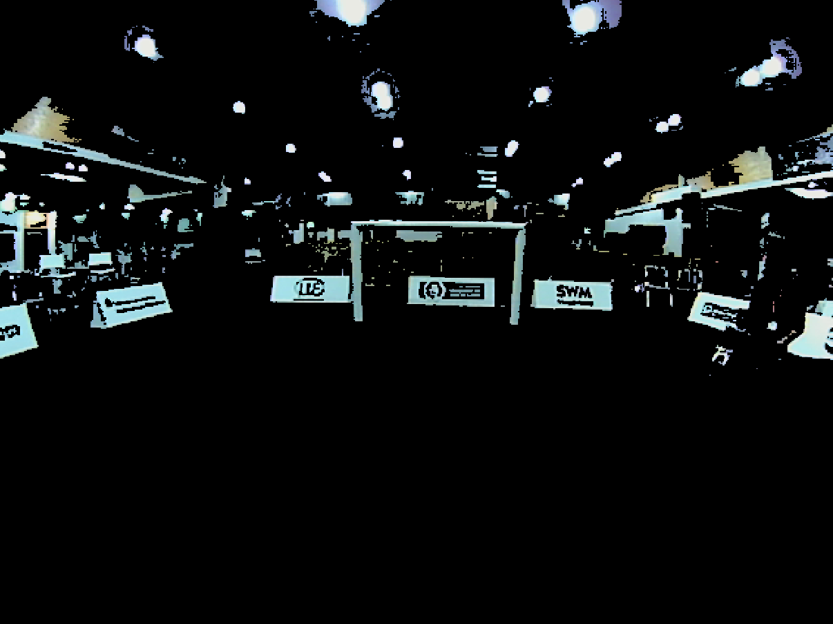
(a) White color segmented image in which pixels that are not considered to be white have been painted black.

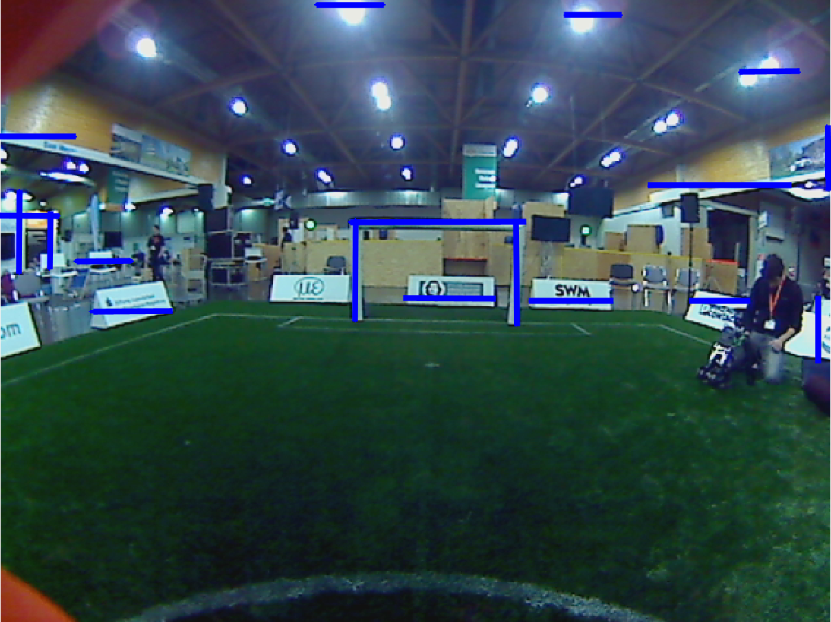
(b) Result after merging all extracted horizontal and vertical white line segments (annotated in blue).

Figure 6: Goal detection on a soccer field.

V-E Obstacle Detection

The rules of the RoboCup humanoid league state that all robots should have mostly black feet. As such, obstacle detection is based on color segmentation of the black color range that is defined by the user. We search for black connected components within the field boundary, and if a detected component is large enough and within a certain predefined distance interval from the robot, the lowest point of the component is returned as the egocentric world coordinates of an obstacle. To prevent the detection of own body parts as obstacles, an image mask is implemented that is dependent on the position of the head. This allows the regions of the image that are expected to contain parts of the own body to be ignored. Using this approach, we are able to detect robots at distances of up to $2\text{\,}\mathrm{m}$.

VI Experimental Results

We used the igus^® Humanoid Open Platform [25] in our experiments. This robot is about $90\text{\,}\mathrm{cm}$ tall and can be used in both the teen-size and kid-size leagues. The robot has a computer with a dual-core AMD E-450 $1.65\text{\,}\mathrm{G}\mathrm{H}\mathrm{z}$ processor and 2GB of memory. This robot is equipped with two 720p Logitech C905 USB cameras. Each camera is fitted with a wide-angle lens that has an infrared cut-off filter, yielding a diagonal field of view of approximately 150^∘. We use the Video4Linux2 library to capture images in RGB format at a resolution of $640\times 480$. So far, we have only evaluated the vision system on one camera at a time. During RoboCup 2015, the computation time of the vision system was measured on the robot. Using only one thread, an average cycle time of $25\text{\,}\mathrm{ms}$ was achieved, with a minimum of $15\text{\,}\mathrm{ms}$, and maximum of $38\text{\,}\mathrm{ms}$, so the proposed vision system can easily run on a single CPU core at $30\text{\,}\mathrm{Hz}$. Of all the components of the vision system, the ball detection is the most time consuming, and the robot detection is the least.

We assessed the performance of the proposed vision system both qualitatively and quantitatively, using an approach similar to that used by Schwarz et al. [9]. As inputs, we used recorded data from the RoboCup German Open 2015, which included captured image data from various different field locations and lighting conditions. The recorded data contained image data, kinematic information and dead-reckoning walking data. Many captured images were affected by motion blur due to walking and head panning motions. The data was evaluated frame by frame by the authors to assess the performance of the vision system in real soccer situations. Table II defines a set of detection criteria for the evaluation of the recorded bags. The success rate of the detections was calculated given the criteria, and the number of false positives was recorded. The results are shown in Table III. Despite the fact that Schwarz et al. tested their vision algorithms in a more color-coded SPL environment [9], we achieve comparable results, and in fact achieve better results when it comes to circle, ball and robot detections. In another comparison of the obtained results, we found that our method outperforms that of Härtl et al. [10] in terms of both line and circle detections, even though their results were obtained in the previous year’s more color-coded RoboCup environment.

In a second experiment, we tested our vision system under various different lighting conditions, including normal, very poor, ambient and natural lighting conditions, without tuning any parameters. The results are shown in Fig. 7. Consistent detections can be seen in all scenarios. We claim that the achieved result is sufficient for successful soccer game play in the new low color information RoboCup environment.

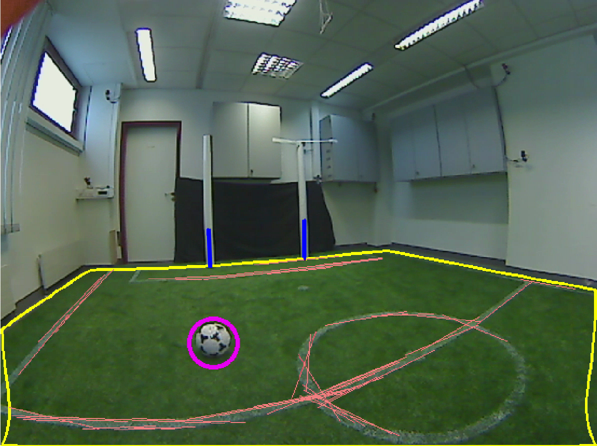
(a) Normal lighting conditions.

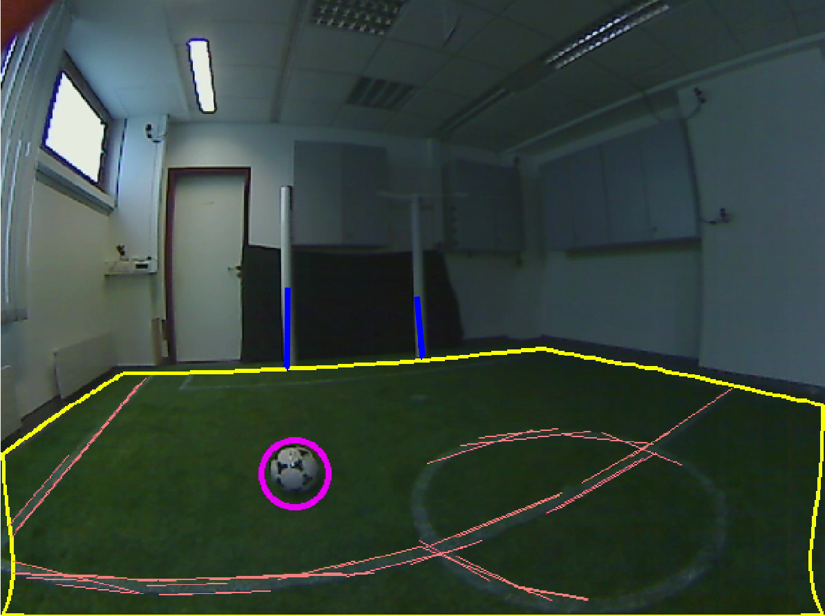
(b) Poor lighting conditions.

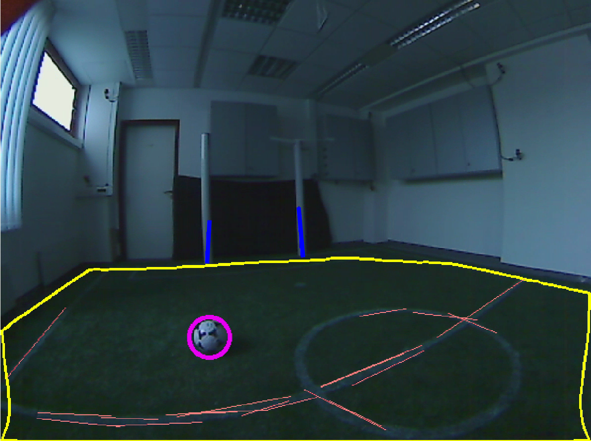
(c) Natural lighting.

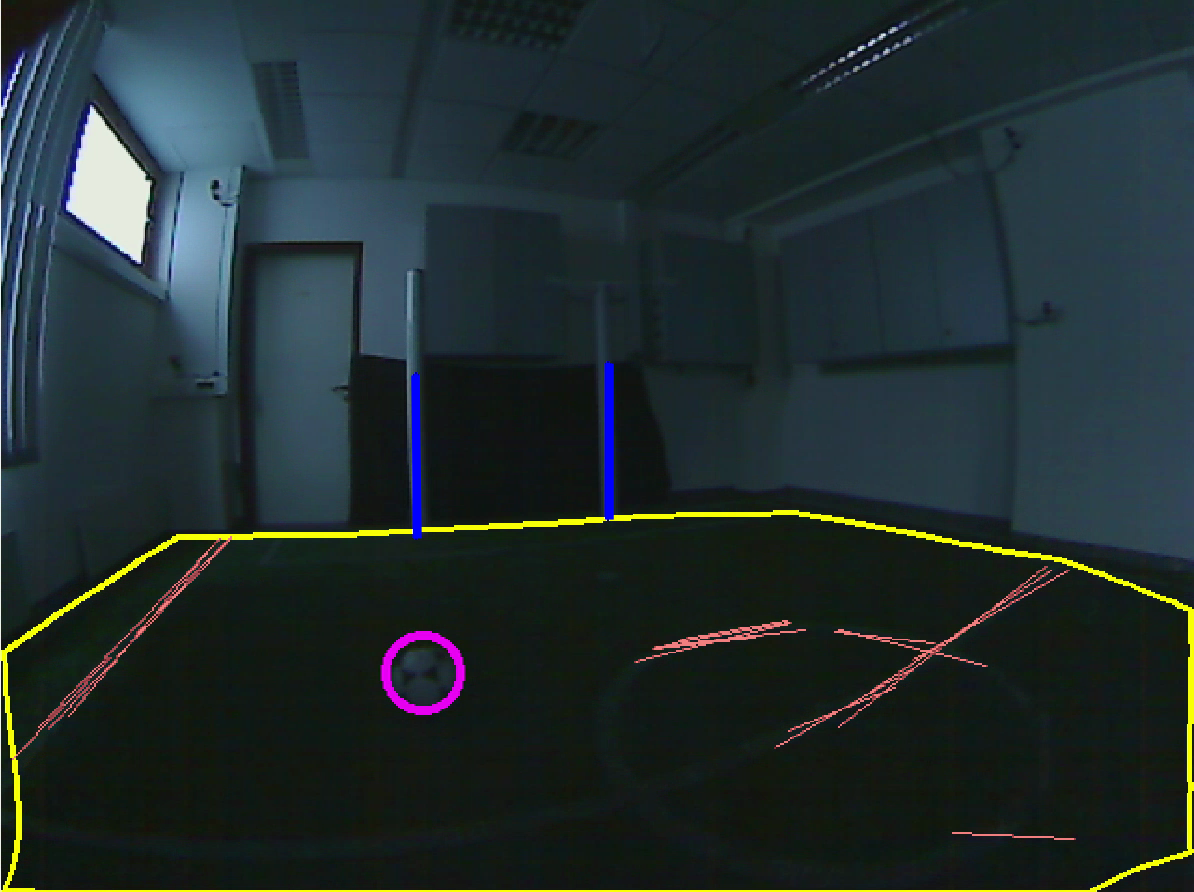
(d) No ambient lighting.

Figure 7: Experimental results under various lighting conditions without any changes in the algorithm parameters.

TABLE II: Evaluation criteria used for feature detections.

Feature	Criteria for expected observability
Field boundary	The field should be visible in the image.
Ball	At least one third of the ball should be visible.
	The ball should be completely within the field boundary at $\leq\,$$4\text{\,}\mathrm{m}$ from the robot.
Field lines	All points of the field line segment should be at most $4.5\text{\,}\mathrm{m}$ from the robot.
	The line segment should be at least $1\text{\,}\mathrm{m}$ in length.
Centre circle	At least one third of the circle should be visible.
Goal posts	The goal post should be $\leq\,$$5\text{\,}\mathrm{m}$ from the robot.
	The base of the goal post should be visible.
	The goal post should have a minimum margin of $30\text{\,}\mathrm{p}\mathrm{x}$ from the edges of the image.
Other robots	The feet of the robot should be completely black and visible.

TABLE III: Detection results for each type of feature.

Feature	Success rate	False positives	Frames
Field boundary	93%	0	1482
Ball	81%	11	457
Field lines	57%	17	187
Centre circle	63%	7	138
Goal posts	48%	3	140
Other robots	71%	0	239

VII Conclusion and Future Work

In this paper, we presented a monocular vision system for humanoid soccer robots that addresses the challenges posed by the new rules of the RoboCup Humanoid League. In order to tackle the challenging task of finding objects in a low color information environment, we proposed a learning approach for ball detection. For detecting goals, field lines, the center circle, and other robots we, proposed effective algorithms with low computational cost. Our methods have been evaluated on data from a RoboCup competition and in lab experiments. The results indicate good detection performance and robustness to changes in lighting conditions.

In the future, we want to increase the maximum distance of ball detection, and utilize stereo vision for better distance estimation. Porting some of the system to run on a GPU is additional future work, along with developing a learning approach for more general robot detection, as the feet of other robots may not always be visible in the image.

References

- [1] R. Gerndt, D. Seifert, J. H. Baltes, S. Sadeghnejad, and S. Behnke, “Humanoid robots in soccer: Robots versus humans in RoboCup 2050,” IEEE Robotics and Automation Magazine, vol. 22, no. 3, pp. 147–154, 2015.
- [2] T. Laue, T. J. De Haas, A. Burchardt, C. Graf, T. Röfer, A. Härtl, and A. Rieskamp, “Efficient and reliable sensor models for humanoid soccer robot self-localization,” in Proceedings of the Fourth Workshop on Humanoid Soccer Robots, 2009, pp. 22–29.
- [3] H. Farazi, M. Hosseini, V. Mohammadi, F. Jafari, D. Rahmati, and E. Bamdad, “Baset Teen-Size 2014 Team Description Paper,” 2014.
- [4] H. Strasdat, M. Bennewitz, and S. Behnke, “Multi-cue localization for soccer playing humanoid robots,” in RoboCup 2006: Robot Soccer World Cup X, ser. Lecture Notes in Computer Science, vol. 4434. Springer, 2007, pp. 245–257.
- [5] H. Schulz and S. Behnke, “Utilizing the structure of field lines for efficient soccer robot localization,” Advanced Robotics, vol. 26, no. 14, pp. 1603–1621, 2012.
- [6] H. Schulz, H. Strasdat, and S. Behnke, “A ball is not just orange: Using color and luminance to classify regions of interest,” in Proceedings of The Second Workshop on Humanoid Soccer Robots, Humanoids Conference, 2007.
- [7] S. Metzler, M. Nieuwenhuisen, and S. Behnke, “Learning visual obstacle detection using color histogram features,” in Proceedings of the 15th RoboCup International Symposium, 2011.
- [8] T. Houliston, M. Metcalfe, and S. K. Chalup, “A fast method for adapting lookup tables applied to changes in lighting colour,” 2015.
- [9] I. Schwarz, M. Hofmann, O. Urbann, and S. Tasse, “A robust and calibration-free vision system for humanoid soccer robots,” 2015.
- [10] A. Härtl, U. Visser, and T. Röfer, “Robust and efficient object recognition for a humanoid soccer robot,” in RoboCup 2013: Robot World Cup XVII. Springer, 2014, pp. 396–407.
- [11] P. Cano, Y. Tsutsumi, C. Villegas, and J. Ruiz-Del-Solar, “Robust detection of white goals,” in RoboCup Symposium, 2015.
- [12] T. Reinhardt, “Kalibrierungsfreie Bildverarbeitungsalgorithmen zur Echtzeitfähigen Objekterkennung im Roboterfußball,” Ph.D. dissertation, 2011.
- [13] G. Bradski, Dr. Dobb’s Journal of Software Tools, 2000.
- [14] P. M. Caleiro, A. J. Neves, and A. J. Pinho, “Color-spaces and color segmentation for real-time object recognition in robotic applications,” Electrónica e Telecomunicações, vol. 4, no. 8, pp. 940–945, 2007.
- [15] T. Foote, “tf: The transform library,” in Technologies for Practical Robot Applications (TePRA), 2013 IEEE International Conference on, ser. Open-Source Software workshop, April 2013, pp. 1–6.
- [16] U. Ramer, “An iterative procedure for the polygonal approximation of plane curves,” Computer graphics and image processing, vol. 1, no. 3, pp. 244–256, 1972.
- [17] N. Dalal and B. Triggs, “Object detection using histograms of oriented gradients,” in Pascal VOC Workshop, ECCV, 2006.
- [18] R. E. Schapire, Y. Freund, P. Bartlett, and W. S. Lee, “Boosting the margin: A new explanation for the effectiveness of voting methods,” Annals of statistics, pp. 1651–1686, 1998.
- [19] D. G. Lowe, “Object recognition from local scale-invariant features,” in The proceedings of the seventh IEEE international conference on Computer Vision, 1999, vol. 2, 1999, pp. 1150–1157.
- [20] C. Vondrick, A. Khosla, T. Malisiewicz, and A. Torralba, “HOGgles: Visualizing Object Detection Features,” ICCV, 2013.
- [21] R. Lienhart and J. Maydt, “An extended set of haar-like features for rapid object detection,” in International Conference on Image Processing, vol. 1, 2002, pp. I–900.
- [22] S. Liao, X. Zhu, Z. Lei, L. Zhang, and S. Z. Li, “Learning multi-scale block local binary patterns for face recognition,” in Advances in Biometrics. Springer, 2007, pp. 828–837.
- [23] J. Canny, “A computational approach to edge detection,” Pattern Analysis and Machine Intelligence, IEEE Transactions on, no. 6, pp. 679–698, 1986.
- [24] J. Matas, C. Galambos, and J. Kittler, “Robust detection of lines using the progressive probabilistic Hough transform,” Computer Vision and Image Understanding, vol. 78, no. 1, pp. 119–137, 2000.
- [25] P. Allgeuer, H. Farazi, M. Schreiber, and S. Behnke, “Child-sized 3D printed igus humanoid open platform,” in Proceedings of 15th IEEE-RAS Int. Conference on Humanoid Robots (Humanoids), 2015.