Plummeting and blinking eigenvalues of the Robin Laplacian in a cuspidal domain

Abstract.

We consider the Robin Laplacian in the domains $\Omega$ and $\Omega^{\varepsilon}$, $\varepsilon>0$, with sharp and blunted cusps, respectively. Assuming that the Robin coefficient $a$ is large enough, the spectrum of the problem in $\Omega$ is known to be residual and to cover the whole complex plane, but on the contrary, the spectrum in the Lipschitz domain $\Omega^{\varepsilon}$ is discrete. However, our results reveal the strange behavior of the discrete spectrum as the blunting parameter $\varepsilon$ tends to 0: we construct asymptotic forms of the eigenvalues and detect families of ”hardly movable” and ”plummeting” ones. The first type of the eigenvalues do not leave a small neighborhood of a point for any small $\varepsilon>0$ while the second ones move at a high rate $O(|\ln\varepsilon|)$ downwards along the real axis ${\mathbb{R}}$ to $-\infty$. At the same time, any point $\lambda\in{\mathbb{R}}$ is a ”blinking eigenvalue”, i.e., it belongs to the spectrum of the problem in $\Omega^{\varepsilon}$ almost periodically in the $|\ln\varepsilon|$-scale. Besides standard spectral theory, we use the techniques of dimension reduction and self-adjoint extensions to obtain these results.

1. Introduction.

1.1. Formulation of the problems.

We consider a family of spectral problems for the Laplace operator with the Robin condition

(1.1) $$-\Delta u^{\varepsilon}(x) = \lambda^{\varepsilon}u^{\varepsilon}(x),\ \ x\in\Omega^{\varepsilon},$$

(1.2) $$\partial_{\nu}u^{\varepsilon}(x) = au^{\varepsilon}(x),\ \ \ x\in\partial\Omega^{\varepsilon},$$

in the domain (Fig. 1.1,b)

(1.3) $$\Omega^{\varepsilon}=\Omega\smallsetminus\overline{\Pi^{\varepsilon}}\subset{\mathbb{R}}^{n}\ ,\ \ n\geq 2,$$

where $\varepsilon\in(0,\varepsilon_{0}]$ is a small parameter, $a\in{\mathbb{R}}$ a constant, $\lambda^{\varepsilon}$ the spectral parameter, $\partial_{\nu}$ is the outward normal derivative,

(1.4) $$\Pi^{d}=\{x=(y,z)\in{\mathbb{R}}^{n-1}\times{\mathbb{R}}\,:\,z=x_{n}\in(0,d),\eta=z^{-2}y\in\omega\}\ ,\ \ d>0,$$

$\omega$ is a domain in ${\mathbb{R}}^{n-1}$ with Lipschitz boundary and compact closure $\overline{\omega}=\omega\cup\partial\omega$, and $\Omega$ is assumed to coincide with the cusp $\Pi^{d}$ in a neighborhood of the coordinate origin ${\mathcal{O}}$ (Fig. 1.1,a). The domain $\Omega$ is Lipschitz everywhere, except at the point ${\mathcal{O}}$.

For $\varepsilon>0$ the domain (1.3) is Lipschitz and the spectrum of the problem (1.1)–(1.2) is discrete, consisting of the monotone increasing unbounded sequence of eigenvalues

(1.5) $$\lambda_{1}^{\varepsilon}<\lambda_{2}^{\varepsilon}\leq\lambda_{3}^{\varepsilon}\leq\ldots\leq\lambda_{m}^{\varepsilon}\leq\ldots\to+\infty.$$

As studied for example in [1], it is possible to define a limit problem ($\varepsilon=0$) in the cuspidal domain $\Omega=\Omega^{0}$,

(1.6) $$-\Delta u(x) = \lambda u(x),\ x\in\Omega\ \ ,\ \ \ \partial_{\nu}u(x)=au(x),\ x\in\partial\Omega,$$

Moreover, it is known that if the constant coefficient in (1.2) is non-positive, this problem has dicrete spectrum. When $a$ is positive, it was proven in [2] that the discrete spectrum constitutes the whole spectrum $\sigma$ of (1.6) only in the case $a<a_{\dagger}$, while $\sigma$ becomes the residual spectrum and covers the whole complex plane ${\mathbb{C}}$ in the case

(1.7) $$a\geq a_{\dagger}=\Big{(}n-\frac{3}{2}\Big{)}^{2}\frac{|\omega|}{|\partial\omega|},$$

where $|\omega|=\mbox{mes}_{n-1}\omega$ is the volume of the cross-section and $|\partial\omega|=\mbox{mes}_{n-2}\partial\omega$ is the area of its boundary.

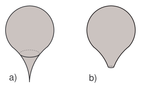
Figure 1.1. Problem domain with a cusp (a) and domain with a blunted csup (b)

1.2. State of art.

When the parameter $a$ is positive, it is not clear how to present a reasonnable weak formulation of the limit problem ($\varepsilon=0$) in the cusp. The Robin Laplacian has been studied in arbitrary domains in different ways. Using a variational approach, a possible start is to consider the quadratic form

$$u\mapsto\|\nabla u;L^{2}(\Omega)\|^{2}-\|a^{1/2}u,L^{2}(\partial\Omega)\|^{2},$$

defined on its natural domain, as shown in [3, Section 3] and [4]. In these works, measures on the boundary are considered, including our case $a>0$. For a domain with a cusp, the resulting operator is not necessarily self-adjoint. If the cusp is, roughly, less sharp than quadratic, then the form is bounded from below, and the spectrum is discrete (see [5, 6, 2] and, e.g., [7] for a recent study of the corresponding eigenvalue sequence itself). But, as it was shown in [6, 2], the nature of the problem operator may become completely different, as it may lose its semi-boundedness, if the cusp is sharper than quadratic, see also [4, Section 5]. For the critical case of a quadratic cusp (1.4) considered here, the spectrum is discrete if and only if $a<a_{\dagger}$, since the spectrum becomes residual and fills in the whole complex plane when $a\geq a_{\dagger}$, see [2].

Let us review the Steklov problem related to (1.1)–(1.2). In the paper [8] it was shown that the spectrum (subset of ${\mathbb{R}}_{+}$) of the Steklov problem in a domain with a peak type boundary singularity is either discrete or may contain a continuous component depending on the sharpness of the peak. Related to this, the linear water wave problem, which contains the Steklov condition on a part of the boundary, was considered in [9] in domains with rotational cusps: a formulation of the problem as a Fredholm operator of index zero was given with the help of appropriate radiation conditions, and it was proven that the continuous spectrum is non-empty and consist of the ray $[\lambda_{\dagger},+\infty)\subset{\mathbb{R}}$ with a certain cut-off point $\lambda_{\dagger}\geq 0$.

The reference [10] contains a study of the Laplace equation

(1.8) $$-\Delta u^{\varepsilon}(x)=0,\ \ x\in\Omega^{\varepsilon},$$

with the spectral Steklov and Dirichlet boundary condition

$$\partial_{\nu}u^{\varepsilon}(x) = \lambda^{\varepsilon}u^{\varepsilon}(x)\ ,\ \ x\in\partial\Omega^{\varepsilon}\smallsetminus\overline{\omega^{\varepsilon}},$$

(1.9) $$u^{\varepsilon}(x) = 0\ ,\ \ x\in\omega^{\varepsilon},$$

where $\omega^{\varepsilon}=\{x\in\Pi^{d}\,:\,x=\varepsilon\}$ is the end of the blunted cusp. The spectrum of this problem is discrete and similar to (1.5). According to [8], the spectrum of the limit Steklov problem ($\varepsilon=0$) in the cuspidal domain $\Omega$ is continuous and equals $[\lambda_{\dagger},+\infty)$ with the cut-off value $\lambda_{\dagger}=a_{\dagger}$, (1.7), while it was discovered in [10] that the eigenvalues $\lambda_{m}^{\varepsilon}>\lambda_{\dagger}$ of the Steklov-Dirichlet in $\Omega^{\varepsilon}$ behave ”strangely” as $\varepsilon\to+0$, namely they ”glide” within the semi-axis $(\lambda_{\dagger},+\infty)$ at a high rate $O(|\ln\varepsilon|)$, which however slows down near $\lambda_{\dagger}$ so as to make $\lambda_{m}^{\varepsilon}$ ”parachute” smoothly on $\lambda_{\dagger}$. Moreover, each point $\lambda>\lambda_{\dagger}$ constitutes a ”blinking” eigenvalue of the problem (1.8), (1.9), namely, for every $\lambda>\lambda_{\dagger}$ there exists a positive sequence $\{\varepsilon_{k}(\lambda)\}_{k=1}^{\infty}$ tending to 0 such that $\lambda$ becomes a true eigenvalue for the problem (1.8), (1.9) in the domain $\Omega^{\varepsilon}$ for some $\varepsilon$ close to $\varepsilon_{k}(\lambda)$, for any $k$. This phenomenon can be used to construct a singular Weyl sequence at $\lambda$ for the Steklov problem operator in $\Omega$, which provides a novel mechanism to form the continuous spectrum from a family of discrete spectra.

1.3. Outline of the paper.

The asymptotic expansions of the solutions of the problem (1.6) near the tip ${\mathcal{O}}$ were derived in detail in [2] and will be reproduced in Sections 2.1–2.3, and although they are the same as in the case of the Steklov problem in [10], the rest of the material is quite different. In Section 2.4 we determine all self-adjoint extensions of the Robin- Laplacian, which is originally defined in the small domain (2.19). However, none of the extensions is lower semi-bounded (for general results on non-semi-bounded sesquilinear, see [11, 12]), which somehow reflects the fact that the spectrum of the problem (1.6) covers the whole complex plane ${\mathbb{C}}$, see [2]. Some of these extensions $A_{\theta_{\bullet}^{\varepsilon}}$ have a peculiar property, namely their eigenfunctions leave a relatively small discrepancy in the Robin condition at the end of the blunted cusp, see Section 4.1, and thus can be regarded as good candidates to model the singularly perturbed problem (1.1), (1.2), cf. the argumentation in [13]. This plan will be realized in Sections 4.2–4.4, where it is shown that a small neighborhood of any point of the spectrum of the extension $A_{\theta_{\bullet}^{\varepsilon}}$ contains an eigenvalue of the problem (1.1), (1.2) in $\Omega^{\varepsilon}$.

An important property is that the extension parameter $\theta_{\bullet}^{\varepsilon}$ in (4.3) is a periodic function in the logarithmic scale $|\ln\varepsilon|$, hence, the spectrum $\sigma(A_{\theta_{\bullet}^{\varepsilon}})$ gains the same property. Among the eigenvalues of $\sigma(A_{\theta_{\bullet}^{\varepsilon}})$ there exist the so called stable eigenvalues, which are hardly movable and are generated by ”trapped modes”, i.e., solutions of the problem (1.6) in the Sobolev space $H^{1}(\Omega)$. However, according to Theorem 3.3 there certainly exist also eigenvalues of $\sigma(A_{\theta_{\bullet}^{\varepsilon}})$ which are generated by ”diffraction” solutions (3.5) of the problem (1.6), move downwards at a high speed along the real axis according to the formulas (3.18) and (4.4), and therefore are called ”plummeting”. In other words, the spectrum $\sigma(A_{\theta_{\bullet}^{\varepsilon}})$ is indeed periodic in $|\ln\varepsilon|$, although as a set only, because some points of it move purposefully to a fixed direction as $\varepsilon\to+0$. Such a situation may occur only in a situation, when the model operator is not lower semi-bounded. This does not happen in the case of the Steklov problem, which is investigated in [10] and characterized by the phenomenon of ”gliding” eigenvalues (see the end of Section 1.2).

2. Theorem on asymptotics in the cuspidal domain.

2.1. Formal asymptotics.

We aim to present the asymptotics of solutions of the problem

(2.1) $$-\Delta u-\lambda u(x) = f(x),\ x\in\Omega,$$

(2.2) $$\partial_{\nu}u-au(x) = 0,\ x\in\partial\Omega,$$

where $a$ satisfies (1.7), and first of all we will describe a formal procedure under the assumptions that the boundary $\partial\omega$ is smooth and the right-hand side $f$ vanishes near the cuspidal tip ${\mathcal{O}}$.

Since the diameter $O(\zeta^{2})$ of the cross-section

$$\omega^{\zeta}=\{(y,z)\in\Pi^{d}\,:\,z=\zeta\}\ ,\ \ 0<\zeta\ll d\ ,$$

is much less than its distance $\zeta$ to the tip ${\mathcal{O}}$, it is logical to accept the standard asymptotic ansatz in thin domains, see e.g. [14, Ch. 14],

(2.3) $$u(x)=w(z)+W(\eta,z)+\ldots,$$

where the dots stand for inessential higher order terms, $\eta=z^{-2}y$ is the ”rapid” variable used in (1.4), and the power-law functions

(2.4) $$w(z)=z^{\mu}w_{0}\ ,\ \ W(\eta,z)=z^{\mu+2}W_{0}(\eta),$$

where $W_{0}\in H^{1}(\omega)$, are to be determined. We insert the ansatz (2.3) into the differential equation (2.1), extract terms of order $z^{\mu-2}$ as $z\to+0$, and thus obtain the relation

(2.5) $$-\Delta_{\eta}W(\eta,z)=z^{4}\partial_{z}^{2}w(z)\ ,\ \ \eta\in\omega.$$

The normal derivative on the lateral side $\Gamma^{d}=\{x\,:\,\eta\in\partial\omega,\ z\in(0,d)\}$ of the cusp $\Pi^{d}$ equals

$$\partial_{\nu}=\big{(}1+4z^{2}|\eta\cdot\nu^{\prime}(\eta)|^{2}\big{)}^{-1/2}\big{(}z^{-2}\nu^{\prime}(\eta)\cdot\nabla_{\eta}-2z\eta\cdot\nu^{\prime}(\eta)\partial_{z}+2(\eta\cdot\nu^{\prime}(\eta))(\eta\cdot\nabla_{\eta})\big{)},$$

where $\nu^{\prime}(\eta)$ is the unit normal vector on the boundary of the domain $\omega\subset{\mathbb{R}}^{n-1}$ and the central dot stands for the scalar product in the Euclidean spaces. Hence, by considering the order $z^{\mu}$ in the boundary condition (2.2), we derive the relation

(2.6) $$\nu^{\prime}(\eta)\cdot\nabla_{\eta}W(\eta,z)=2\eta\cdot\nu^{\prime}(z)z^{3}\partial_{z}w(z)+az^{2}w(z)\ ,\ \ \eta\in\partial\omega.$$

Using the formula

$$\int\limits_{\partial\omega}\eta\cdot\nu^{\prime}(\eta)ds_{\eta}=\int\limits_{\omega}\nabla_{\eta}\cdot\eta\,d\eta=(n-1)|\omega|$$

we see that the compatibility condition in the Neumann problem (2.5), (2.6) reads as

$$0 = \int\limits_{\omega}\partial_{z}^{2}w(z)d\eta+\int\limits_{\partial\omega}\big{(}2\eta\cdot\nu^{\prime}(\eta)z^{3}\partial_{z}w(z)+az^{2}w(z)\big{)}ds_{\eta}$$

$$= |\omega|\partial_{z}^{2}w(z)+2(n-1)|\omega|z^{3}\partial_{z}w(z)+az^{2}|\partial\omega|w(z)$$

and turns into the ordinary differential equation of Euler type

(2.7) $$-\frac{d}{dz}\Big{(}z^{2(n-1)}\frac{dw}{dz}(z)\Big{)}=Az^{2(n-2)}w(z)\ ,\ \ z>0,$$

where

$$A=a\frac{|\partial\omega|}{|\omega|}.$$

The general solution of the equation (2.7) is of the form

(2.8) $$w(z)=b_{+}w^{+}(z)+b_{-}w^{-}(z)\ ,\ \ b_{\pm}\in{\mathbb{C}},$$

where we have in the case $a>a_{\dagger}$, (1.7),

(2.9) $$w^{\pm}(z)=w_{0}z^{\pm i\mu_{0}-n+3/2}\ \ \mbox{with}\ \mu_{0}=\sqrt{A-\Big{(}n-\frac{3}{2}\Big{)}^{2}}>0\ ,$$

and in the case $a=a_{\dagger}$, $A=(n-3/2)^{2}$

(2.10) $$w^{\pm}(z)=w_{0}z^{-n+3/2}\big{(}\ln z\mp i\big{)}.$$

The normalization factor $w_{0}$ and the peculiar form of (2.10) will be clarified later on.

Since the compatibility condition in the problem (2.5)–(2.6) is fulfilled, there exists a solution $W$ defined up to an additive constant with respect to $\eta$. To make the solution unique, we impose the orthogonality condition

(2.11) $$\int\limits_{\omega}W(\eta,z)d\eta=0.$$

2.2. Weak formulation of the problem.

We introduce the weighted Sobolev space $V_{\beta}^{1}(\Omega)$ as the completion of the linear space $C_{c}^{\infty}(\overline{\Omega}\smallsetminus{\mathcal{O}})$ (infinitely differentiable functions vanishing in a neighborhood of the point ${\mathcal{O}}$) with respect to the norm

(2.12) $$\|u;V_{\beta}^{1}(\Omega)\|=\big{(}\|r^{\beta}\nabla u;L^{2}(\Omega)\|^{2}+\|r^{\beta-1}u;L^{2}(\Omega)\|^{2}\big{)}^{1/2}$$

where $r={\rm dist}\,(x,{\mathcal{O}})$ and $\beta\in{\mathbb{R}}$ is a weight index. The weighted Lebesgue space $V_{\beta}^{0}(\Omega)$ is endowed with the norm $\|r^{\beta}u;L^{2}(\Omega)\|$.

Remark 2.1.

The norm (2.12) is the same as the classical Kondratiev norm [15], but the reason for the use of this norm in [2] as well as in the present paper is not the conventional one, since the shape of the domain $\Omega$ near the singularity point ${\mathcal{O}}$ is not conical nor angular as in Kondratiev’s works. This can be seen for example in the asymptotic ansatz for solutions: $W_{0}$ being in $H^{1}(\omega)$, the sum $w(z)+W(z^{-2}y,z)$, see (2.4), belongs to $V_{\beta}^{1}(\Pi^{d})$, if and only if

$$\beta>-{\rm Re}\,\mu-n+3/2$$

even in the case $w=0$. However, if $w=0$ and $W_{0}(\eta)$ is independent of the fast variable $\eta=z^{-2}y$, the condition for the space $V_{\beta}^{1}(\Pi^{d})$ to include $W$ becomes much less restrictive:

$$\beta>-{\rm Re}\,\mu-n-1/2.\hfill\hskip 56.9055pt\boxtimes$$

According to [2], the weak formulation of the problem (2.1)-(2.2) for the unknown $u\in V_{\beta}^{1}(\Omega)$ reads as the integral identity

(2.13) $$(\nabla u,\nabla v)_{\Omega}-\lambda(u,v)_{\Omega}-a(u,v)_{\Omega}=f(v)\ \ \ \forall\,v\in V_{-\beta}^{1}(\Omega),$$

where $f\in V_{-\beta}^{1}(\Omega)^{*}$ is an (anti)linear functional on $V_{-\beta}^{1}(\Omega)$, in particular

(2.14) $$f(v)=(f,v)_{\Omega}\ \ \ \mbox{with}\ f\in V_{\beta+1}^{0}(\Omega).$$

Here $(\cdot,\cdot)_{\Omega}$ is the natural scalar product in $L^{2}(\Omega)$, extended by density to the duality between the spaces $V_{\beta}^{0}(\Omega)$ and $V_{-\beta}^{0}(\Omega)$. According to definition (2.12) and the weighted trace inequality [2, Lemma 2.2]

$$\|r^{\beta}u;L^{2}(\partial\Omega)\|\leq c\|u;V_{\beta}^{1}(\Omega)\|,$$

all expressions in the integral identity (2.13) are properly defined so that it determines a continuous mapping

$$V_{\beta}^{1}(\Omega)\ni u\mapsto{\mathcal{T}}_{\beta}(\lambda)u=f\in V_{-\beta}^{1}(\Omega)^{*}.$$

We observe that for every $\beta$, ${\mathcal{T}}_{-\beta}(\lambda)$ is the adjoint operator of ${\mathcal{T}}_{\beta}(\lambda)$. In Section 3 we use the arguments of [2] to describe the properties of ${\mathcal{T}}_{\pm\beta}(\lambda)$ in the particular case $\beta=1$.

2.3. Theorem on asymptotics.

We consider the problem (2.1)–(2.2) with the right-hand side

(2.15) $$f\in L^{2}(\Omega)\subset V_{-1}^{1}(\Omega)^{*}\ \$$

(i.e. $\beta=-1$ in (2.14)) and its solution $u\in V_{1}^{1}(\Omega)\subset L^{2}(\Omega).$

The following assertion was verified in [2].

Theorem 2.2.

If (1.7) and (2.15) hold true, the above mentioned solution has the asymptotic form

(2.16) $$u(x)=\chi(x)\big{(}w(z)+W(z^{-2}y,z)\big{)}+\widetilde{u}(x),$$

where $\chi$ is a smooth cut-off function which is equal to $1$ in $\Pi^{d/2}$ and $0$ in $\Omega^{d}$, see (1.4) and (1.3). The term $w$ in (2.16) is the linear combination (2.8) with some coefficients $b_{\pm}$ and terms (2.9) or (2.10), and $W\in H^{1}(\Omega)$ is the solution of the problem (2.5), (2.6), (2.11). The coefficients $b_{\pm}$ and the remainder $\widetilde{u}\in V_{-1}^{1}(\Omega)$ satisfy the estimate

(2.17) $$\big{(}|b_{+}|^{2}+|b_{-}|^{2}+\|\widetilde{u};V_{-1}^{1}(\Omega)\|^{2}\big{)}^{1/2}\leq c\big{(}\|f;L^{2}(\Omega)\|+\|u;V_{1}^{1}(\Omega)\|\big{)},$$

here the factor $c>0$ is independent of $f$ and $u$.

Remark 2.3.

According to formulas (2.9), (2.10) and Remark 2.1, the detached asymptotic term on the right of (2.16) belongs to the space $V_{\gamma}^{1}(\Omega)$ with any $\gamma>0$, but it is not contained in $V_{-1}^{1}(\Omega)$. Furthermore, as for second derivatives we have $\nabla^{2}w\in V_{\gamma+1}^{0}(\Pi^{d})$ and $\nabla^{2}W\in V_{\gamma+2}^{0}(\Pi^{d})$, but in general $\nabla^{2}W\notin V_{\gamma+1}^{0}(\Pi^{d})$. As it was verified in [2], for the solution $u$ there holds $\nabla^{2}u\in V_{1+2}^{1}(\Omega)$ and $\nabla^{2}\widetilde{u}\in V_{-1+2}^{1}(\Omega)$. We emphasize that the term $W$, generated by (2.9), (2.8) and (2.6) is defined up to the addendum

$$b_{+}^{0}z^{+i\mu-n+7/2}+b_{-}^{0}z^{-i\mu-n+7/2}$$

which is independent of $\eta$ and belongs to $V_{1}^{1}(\Omega)$ and can therefore be omitted in the asymptotic representation (2.16); this was the very reason for imposing the orthogonality condition (2.11).

All these peculiarities again underline the difference of the conical [15] and cuspidal [2] irregularities of boundaries.

By ${\bf V}_{\pm 1}^{1}(\Omega)$ we denote the weighted space with detached asymptotics (see [16, Ch. 6], [17, Sect. 3] and others), which consists of functions of the form (2.16) and endow it with the norm on the left of (2.17); the Hilbertian structure of this norm can also be identified with the direct product

(2.18) $${\mathbb{C}}^{2}\times V_{-1}^{1}(\Omega)\ni(b_{\pm},\widetilde{u}),$$

although these will not be used later on.

2.4. Symmetric and self-adjoint operators.

As in [9] we associate to the problem (2.1)–(2.2) the symmetric operator ${\mathcal{A}}$ in $L^{2}(\Omega)$, which has the differential expression $-\Delta$ and the domain

(2.19) $${\mathcal{D}}({\mathcal{A}})=\{u\in V_{-1}^{1}(\Omega)\,:\,\Delta u\in L^{2}(\Omega),\ \partial_{n}u=au\ \mbox{on}\ \partial\Omega\smallsetminus{\mathcal{O}}\}.$$

Notice that the inclusions in (2.19) assure that $u\in H^{2}(\overline{\Omega}\smallsetminus{\mathcal{O}})$ and therefore the trace of $\partial_{n}u$ is properly defined on $\partial\Omega\smallsetminus{\mathcal{O}}$. By Theorem 2.2, see also [2, Prop. 3.11], the adjoint operator ${\mathcal{A}}^{*}$ has the same differential expression but a larger domain

$${\mathcal{D}}({\mathcal{A}}^{*})=\{u\in V_{1}^{1}(\Omega)\,:\,\Delta u\in L^{2}(\Omega),\ \partial_{n}u=au\ \mbox{on}\ \partial\Omega\smallsetminus{\mathcal{O}}\}.$$

In view of Theorem 2.2 on asymptotics, the dimension of the quotient space ${\mathcal{D}}({\mathcal{A}}^{*})/{\mathcal{D}}({\mathcal{A}})$ equals 2.

In order to describe the self-adjoint extensions of the operator ${\mathcal{A}}$ we reproduce a calculation from [2, §3.4]. Let $\zeta>0$. Applying the Green formula in the domain $\Omega^{\zeta}$ for $u^{1}$, $u^{2}\in{\mathcal{D}}({\mathcal{A}}^{*})$ and sending $\zeta$ to $+0$, we get

(2.20) $$({\mathcal{A}}^{*}u^{1},u^{2})_{\Xi}-(u^{1},{\mathcal{A}}^{*}u^{2})_{\Xi}$$

$$= \lim\limits_{\zeta\to+0}\int\limits_{\omega^{\zeta}}\big{(}\overline{u^{2}(y,z)}\partial_{z}u^{1}(y,z)-u^{1}(y,z)\overline{\partial_{z}u^{2}(y,z)}\big{)}\Big{|}_{z=\zeta}dy.$$

Substituting $V_{\beta}^{1}(\Omega)\ni u^{j}\mapsto\widetilde{u}^{j}\in V_{-\beta}^{1}(\Omega)$ at least for one of the indices $j=1,2$ makes the limit on the right of (2.20) equal to zero. Hence, we can replace $u^{j}$ by $w^{j}+W^{j}$ in the representation formula (2.16). Furthermore, since $W^{j}$ has the additional factor $z^{2}$, cf. (2.4), we can neglect the second term in this sum and write

$$({\mathcal{A}}^{*}u^{1},u^{2})_{\Xi}-(u^{1},{\mathcal{A}}^{*}u^{2})_{\Xi}$$

$$= \lim\limits_{\zeta\to+0}\zeta^{2(n-1)}\int\limits_{\omega}\big{(}\overline{w^{2}(\zeta)}\partial_{z}w^{1}(\zeta)-w^{1}(\zeta)\overline{\partial_{z}w^{2}(\zeta)}\big{)}d\eta.$$

Finally, we fix the normalization factor in (2.9) and (2.10),

$$w_{0}=\left\{\begin{array}[]{ll}\sqrt{2\mu_{0}|\omega|}&\mbox{for}\ a>a_{\dagger},\\ \sqrt{2|\omega|}&\mbox{for}\ a=a_{\dagger},\end{array}\right.$$

and obtain

(2.21) $$({\mathcal{A}}^{*}u^{1},u^{2})_{\Xi}-(u^{1},{\mathcal{A}}^{*}u^{2})_{\Xi}=i\big{(}\overline{b_{+}^{2}}b_{+}^{1}-\overline{b_{-}^{2}}b_{-}^{1}\big{)},$$

where $b_{\pm}^{j}$ are the coefficients of the linear combination $w_{j}$, see (2.8). Repeating a traditional argument in [18] we observe that if $u^{1}$ and $u^{2}$ belong to the domain of a self-adjoint operator, then the left-hand side of (2.21) vanishes and thus the coefficients must be related as $b_{-}^{j}=e^{i\theta}b_{+}^{j}$ for some $\theta\in[0,2\pi)$.

Theorem 2.4.

The restriction ${\mathcal{A}}_{\theta}$, where $\theta\in[0,2\pi)$, of the operator ${\mathcal{A}}^{*}$ to the subspace

(2.22) $$\big{\{}u\in{\mathcal{D}}({\mathcal{A}}^{*})\,:\,b_{+}=e^{i\theta}b_{-}\big{\}}$$

is a self-adjoint extension of the operator ${\mathcal{A}}$. Moreover, the domain of any self-adjoint extension of ${\mathcal{A}}$ equals (2.22) for some parameter $\theta\in[0,2\pi)$.

3. Spectra of self-adjoint extensions.

3.1. Operator kernels.

We fix the parameter $\lambda$, assume (1.7), and compare $\lambda$ and compare the Fredholm operators ${\mathcal{T}}_{+1}(\lambda)$ and ${\mathcal{T}}_{-1}(\lambda)$, which are adjoint to each other and therefore

(3.1) $${\rm dim\,ker}\,{\mathcal{T}}_{\pm 1}(\lambda)={\rm dim\,coker}\,{\mathcal{T}}_{\mp 1}(\lambda)\ \ \Rightarrow\ \ {\rm Ind}\,{\mathcal{T}}_{+1}(\lambda)=-{\rm Ind}\,{\mathcal{T}}_{-1}(\lambda).$$

Clearly, $V_{-1}^{1}(\Omega)\subset V_{+1}^{1}(\Omega)$ and

(3.2) $${\rm ker}\,{\mathcal{T}}_{-1}(\lambda)\subset{\rm ker}\,{\mathcal{T}}_{+1}(\lambda).$$

Furthermore, Theorem 2.2 on asymptotics shows that

(3.3) $${\rm Ind}\,{\mathcal{T}}_{+1}(\lambda)=2+{\rm Ind}\,{\mathcal{T}}_{-1}(\lambda)$$

where 2 is nothing but the number of the detached terms in formula (2.16), see (2.8) with free constants $b_{\pm}$. From (3.1) and (3.3) we deduce that Ind ${\mathcal{T}}_{\pm}(\lambda)=\pm 1$, and taking (3.2) into account yields

$${\rm ker}\,{\mathcal{T}}_{+1}(\lambda)={\rm ker}\,{\mathcal{T}}_{-1}(\lambda)\oplus{\mathcal{Z}},\ \ \ {\rm dim}\,{\mathcal{Z}}=1.$$

Any non-zero function $Z\in{\mathcal{Z}}={\rm ker}\,{\mathcal{T}}_{+1}(\lambda)\ominus{\rm ker}\,{\mathcal{T}}_{-1}(\lambda)$, i.e. a solution of the homogeneous problem (2.1)–(2.2) belonging to $V_{1}^{1}(\Omega)$, has the representation (2.16) with the linear combination (2.8); the generalized Green formula (2.21) with $u^{1}=u^{2}=Z$ yields the equality

(3.4) $$0=i|b_{+}|^{2}-i|b_{-}|^{2}.$$

If $b_{\pm}=0$, we arrive at the contradiction

$$Z\in V_{-1}^{1}(\Omega)\ \ \Rightarrow\ \ Z\in{\rm ker}\,{\mathcal{T}}_{-1}(\lambda).$$

Thus, none of the coefficients vanishes and in view of (3.4) we can choose a particular solution

(3.5) $$Z_{\lambda}(x) = \chi(x)\big{(}w_{-}(z)+W_{-}(z^{-2}y,z)+e^{i\Theta(\lambda)}\big{(}w_{+}(z)+W_{+}(z^{-2}y,z)\big{)}$$

$$+ \widetilde{Z}_{\lambda}(x).$$

where $\Theta(\lambda)\in[0,2\pi)$ and $\widetilde{Z}_{\lambda}\in V_{-1}^{1}(\Omega)$.

Remark 3.1.

The singular functions (2.9) and (2.10) can be interpreted as ”waves” travelling along the axis of the cusp, cf. [9] for a physical argument in a similar geometric situation. Although such an interpretation is not directly needed in our paper, it is convenient to use the corresponding physical terminology, namely to call solutions in ker ${\mathcal{T}}_{-1}(\lambda)$ ”trapped modes” and to consider $e^{i\Theta(\lambda)}$ as the ”scattering coefficient” in the ”diffraction” solution (3.5).   $\boxtimes$

All functions $u\in{\rm ker}\,{\mathcal{T}}_{1}(\lambda)\subset V_{1}^{1}(\Omega)\subset L^{2}(\Omega)$ belong to the domain (2.20) of ${\mathcal{A}}^{*}$, because the inclusion $\Delta u=-\lambda u\in L^{2}(\Omega)$ really occurs. Hence, a trapped mode is an eigenvector corresponding to its eigenvalue $\lambda$ for every self-adjoint operator ${\mathcal{A}}_{\theta}$ of Theorem 2.4. Furthermore, it can readily be seen that in the case $\theta=\Theta(\lambda)$ there appears a second eigenvector (3.5) of ${\mathcal{A}}_{\theta}$.

3.2. Examples of trapped modes.

Following the ideas of [19] and [8] we assume that the domain $\Omega$ is mirror symmetric with respect to the plane $\{x_{1}=0\}$, i.e.,

(3.6) $$\Omega=\{x\,:\,(-x_{1},x_{2},\ldots,x_{n})\in\Omega\}$$

and restrict the problem (2.1)–(2.2) with $f=0$ to the half $\Omega_{+}=\{x\in\Omega\,:\,x_{1}>0\}$ of the domain (3.6),

(3.7) $$-\Delta u_{+}(x) = \lambda_{+}u_{+}(x),\ x\in\Omega_{+}\ ,$$

(3.8) $$\partial_{\nu}u_{+}(x) = au_{+}(x),\ x\in(\partial\Omega)_{+}=\partial\Omega_{+}\setminus\overline{\Sigma},$$

where we impose the artificial Dirichlet condition

(3.9) $$u_{+}(x)=0\ \ ,\ \ \ x\in\Sigma,$$

on the middle plane $\Sigma=\{x\in\Omega\,:\,x_{1}=0\}$.

Lemma 3.2.

Assume that the function $u_{+}\in H_{\rm loc}^{1}(\overline{\Omega_{+}}\smallsetminus{\mathcal{O}})$ satisfies the inclusion $\nabla u_{+}\in L^{2}(\Omega_{+})$ and the Dirichlet condition (3.9). Then, the following weighted inequality is valid:

(3.10) $$\|r^{-2}u_{+};L^{2}(\Omega_{+})\|+\|r^{-1}u_{+};L^{2}((\partial\Omega)_{+})\|\leq c\|\nabla u_{+};L^{2}(\Omega_{+})\|.$$

Proof. It suffices to verify (3.10) in the cusp $\Pi_{+}^{d}=\{x\in\Pi^{d}\,:\,x_{1}>0\}$ and on the surface $\Gamma_{+}^{d}=\{x\in\Gamma^{d}\,:\,x_{1}>0\}$. To this end, we write lower-dimensional inequalities in the half-section $\omega_{+}^{\zeta}=\{y\in\omega^{\zeta}\,:\,y_{1}>0\}$,

$$\zeta^{-4}\int\limits_{\omega_{+}^{\zeta}}|u_{+}(y,\zeta)|^{2}dy\leq c\int\limits_{\omega_{+}^{\zeta}}\big{|}\nabla_{y}u_{+}(y,\zeta)\big{|}^{2}dy$$

(3.11) $$\zeta^{-2}\int\limits_{\partial\omega_{+}^{\zeta}}|u_{+}(y,\zeta)|^{2}ds_{y}\leq c\int\limits_{\omega_{+}^{\zeta}}\big{|}\nabla_{y}u_{+}(y,\zeta)\big{|}^{2}dy$$

coming from the Dirichlet condition (3.9) and the coordinate dilatation $y\mapsto\eta=\zeta^{-2}y$. The proof is completed by integrating (3.11) in $\zeta\in(0,d)$ and taking into account that $ds_{x}=\big{(}1+4z^{2}|\eta\cdot\nu^{\prime}(\eta)|^{2}\big{)}^{1/2}ds_{y}dz$.   $\boxtimes$

The variational formulation of the problem (3.8)–(3.9),

(3.12) $$(\nabla_{x}u_{+},\nabla_{x}v_{+})_{\Omega_{+}}-a(u_{+},v_{+})_{(\partial\Omega)_{+}}=\lambda(u_{+},v_{+})_{\Omega_{+}}\ \ \forall\,v_{+}\in H_{0}^{1}(\Omega_{+};\Sigma)$$

is posed in the Sobolev space $H_{0}^{1}(\Omega_{+};\Sigma)\subset H^{1}(\Omega)$ of functions vanishing on $\Sigma$. Since the weight $r^{-1}$ in the second norm of (3.10) is large when $x\to{\mathcal{O}}$, the embedding $H^{1}_{0}(\Omega_{+},\Sigma)\subset L^{2}(\Omega_{+})$ is compact, and therefore the whole left-hand side of (3.12) is lower semi-bounded. We deduce that the spectrum of the variational problem (3.12) or the differential problem (3.8)–(3.9) is discrete and consists of the monotone unbounded sequence of normal eigenvalues

(3.13) $$\lambda_{+}^{1}<\lambda_{+}^{2}\leq\lambda_{+}^{3}\leq\ldots\leq\lambda_{+}^{m}\leq\ldots\to+\infty.$$

The corresponding eigenfunctions $u_{+}^{m}\in H_{0}^{1}(\Omega_{+},\Sigma)$, $m=1,2,,\ldots$, have smooth, odd extensions over the Dirichlet surface $\Sigma$ to $\Omega$. The extensions belong to $H^{1}(\Omega)$ and thus become eigenfunctions of the original problem (1.6), due to the symmetry of the domain (3.6). Using (3.10) we conclude that the extended eigenfunctions $u^{m}$ belong to $V_{-2}^{0}(\omega)$ and therefore to $V_{-1}^{1}(\Omega)$, by Theorem 2.6 of [2]. In this way the eigenvalues (3.13) are embedded into the residual spectrum of the operator ${\mathcal{A}}$. They also belong to the point spectrum of any self-adjoint extension ${\mathcal{A}}_{\theta}$ of Theorem 2.4.

It would be possible to show, using a general result of [20, 21], that the eigenfunctions of the problem (1.6) belonging to $V_{-1}^{1}(\omega)$ decay exponentially as $O(e^{-\delta/r})$ for some $\delta>0$, although this argument would require lengthy additional computations contained in [22, Ch. 10] and [2, Sect.1.5]. However, Theorem 2.6 of [2], the proof of which is much simpler, directly implies that a solution $u$ of (1.6) belongs to $\in V_{-\beta}^{1}(\Omega)$ for all $\beta\in{\mathbb{R}}_{+}$, i.e., it gets a super-power decay rate, which will be sufficient for our purposes.

3.3. A peculiar property of the scattering coefficient.

Let us consider the solution $Z_{\lambda+\delta}$ of (1.6), when $\lambda$ is replaced by the perturbation $\lambda+\delta$, where $\delta$ is a small parameter with an arbitrary sign. We accept the simplest asymptotic ansätze with respect to small $\delta$ for this solution and its scattering coefficient:

(3.14) $$Z_{\lambda+\delta}(x) = Z_{\lambda}(x)+\delta Z_{\lambda}^{\prime}(x)+\widehat{Z}_{\lambda+\delta}(x),$$

$$\Theta(\lambda+\delta) = \Theta(\lambda)+\delta\Theta^{\prime}(\lambda)+\widehat{\Theta}(\lambda+\delta).$$

Both $Z_{\lambda+\delta}$ and $\Theta(\lambda+\delta)$ depend smoothly on $\delta$, so that we only need to compute the correction terms, while the estimates of the remainders are evident due to the general perturbation theory, cf. [23].

We derive the following problem for the function $Z_{\lambda}^{\prime}$ by inserting (3.14) to (1.6) with $\lambda\mapsto\lambda+\delta$ and extracting terms of order $O(\delta)$:

$$-\Delta Z_{\lambda}^{\prime}(x)-\lambda Z_{\lambda}^{\prime}(x) = Z_{\lambda}(x)\ \ ,\ \ x\in\Omega,$$

(3.15) $$\partial_{\nu}Z_{\lambda}^{\prime}(x) = aZ_{\lambda}^{\prime}(x)\ \ ,\ \ x\in\partial\Omega\smallsetminus{\mathcal{O}}.$$

Using the formulas (3.5) with $\lambda$ and $\lambda\mapsto\lambda+\delta$, and the Taylor formula

$$e^{i\Theta(\lambda+\delta)}=e^{i\Theta(\lambda)}\big{(}1+i\delta\Theta^{\prime}(\lambda)+O(\delta^{2})\big{)},$$

we derive the representation

(3.16) $$Z_{\lambda}^{\prime}(x)=i\Theta^{\prime}(\lambda)e^{i\Theta(\lambda)}\chi(x)\big{(}w_{+}(z)+W_{\dagger}(z^{-2}y,z)\big{)}+\widetilde{Z}_{\lambda}^{\prime}(x)$$

where $\widetilde{Z}_{\lambda}^{\prime}\in V_{-1}^{1}(\Omega)$ and the incoming wave $w_{-}$ does not appear. The problem (3.15) has a solution of the form (3.16). Indeed, since the solution (3.5) is originally defined up to a trapped mode in ker ${\mathcal{T}}_{-1}(\lambda)$, the orthogonality conditions

(3.17) $$(Z_{\lambda},v)_{\Omega}=0\ \ \ \forall\,v\in{\rm ker}\,{\mathcal{T}}_{-1}(\lambda)$$

can be satisfied, and because of the Fredholm property of ${\mathcal{T}}_{\pm 1}(\lambda)$, they guarantee the existence of a solution of the problem (3.15) belonging to $V_{1}^{1}(\Omega)$; the solution is defined up to an addentum in ker ${\mathcal{T}}_{1}(\lambda)$, in particular, up to the term $c_{\lambda}Z_{\lambda}$. By Theorem 2.2, this general solution has the representation (2.16) with $w=b_{+}(\lambda)w_{+}+b_{-}(\lambda)w_{-}$, see (2.8). Setting $c_{\lambda}=-b_{-}(\lambda)$ gives (3.16) and the orthogonality conditions (3.17).

We now insert the functions $Z_{\lambda}^{\prime}$ and $Z_{\lambda}$ into Green’s formula in $\Omega^{\zeta}$ and take the limit $\zeta\to+0$ as in (2.20) and (2.21). The inhomogeneous equation in (3.15) implies

$$\|Z_{\lambda};L^{2}(\Omega)\|^{2}=\lim\limits_{\zeta\to+0}\|Z_{\lambda};L^{2}(\Omega^{\zeta})\|^{2}$$

$$= -\lim\limits_{\zeta\to+0}\int\limits_{\omega^{\zeta}}\big{(}\overline{Z_{\lambda}(y,\zeta)}\partial_{z}Z_{\lambda}^{\prime}(y,\zeta)-Z_{\lambda}^{\prime}(y,\zeta)\partial_{z}\overline{Z_{\lambda}(y,\zeta)}\big{)}dy$$

$$= i\big{(}-1\cdot 0+\overline{e^{i\Theta(\lambda)}}i\Theta^{\prime}e^{i\Theta(\lambda)}\big{)}=-\Theta^{\prime}.$$

Let us formulate the result.

Theorem 3.3.

There holds the formula

(3.18) $$\partial_{\lambda}\Theta(\lambda)=-\|Z_{\lambda};L^{2}(\Omega)\|^{2}<0,$$

where $Z_{\lambda}$ is the solution (3.5) of the problem (1.6), with (1.7), subject to the subject to the orthogonality conditions (3.17).

The relation (3.18) means that the growth of the spectral parameter $\lambda$ in (3.16) makes the scattering coefficient $e^{i\Theta(\lambda)}$ run along the unit circle $\{z\in{\mathbb{C}}\,:\,|z|=1\}$ counter-clockwise. Unfortunately, our calculation does not allow to control the running speed, because the solution $Z_{\lambda}$ is normalized by the unit coefficient of the incoming wave $w_{+}$, while the norm $\|Z_{\lambda};L^{2}(\Omega)\|$ depends on the function $Z_{\lambda}$ in the whole domain.

4. Asymptotics of eigenvalues in the domain with a blunted cusp.

4.1. Formal procedure.

We consider a solution of the limit problem (1.6), with (1.7), of the form (2.16) and use the coefficients $b_{\pm}$ in (2.8) to satisfy the boundary condition (1.2) at the end $\omega^{\varepsilon}$ of the blunted cusp (1.3). We denote here by dots terms which are inessential for our present asymptotic analysis and postpone their estimates to the next sections.

In the case $a>a_{\dagger}$ we apply formulas (2.9), (2.6) and obtain

(4.1) $$\partial_{\nu}u(y,\varepsilon)+au(y,\varepsilon) = w_{0}\Big{(}+i\mu_{0}-n+\frac{3}{2}+\varepsilon a\Big{)}b_{+}\varepsilon^{+i\mu_{0}-n+1/2}$$

$$+ w_{0}\Big{(}-i\mu_{0}-n+\frac{3}{2}+\varepsilon a\Big{)}b_{-}\varepsilon^{-i\mu_{0}-n+1/2}+\ldots.$$

Hence, the main asymptotic term in (4.1) vanishes provided

(4.2) $$b_{+}=B(\varepsilon)b_{-}\ \ ,\ \ B(\varepsilon)=\frac{-i\mu_{0}+\varepsilon a-n+3/2}{+i\mu_{0}+\varepsilon a-n+3/2}\varepsilon^{-2i\mu_{0}}.$$

The coefficient $B(\varepsilon)$ is unimodular and thus

(4.3) $$B(\varepsilon)=e^{iT(\varepsilon)}\ \ ,\ \ T(\varepsilon)=T_{0}(\varepsilon)-2\mu_{0}\ln\varepsilon,$$

where $T_{0}(\varepsilon)$ is a smooth function of $\varepsilon$ and $\mu_{0}$ is as in (2.9) (notice that $\mu_{0}=0$ for $a=a_{\dagger}$). Comparing (4.2), (4.3) with (2.22), we see that the self-adjoint extension ${\mathcal{A}}_{\theta_{\bullet}^{\varepsilon}}$ of Theorem 2.4, with the parameter

(4.4) $$\theta_{\bullet}^{\varepsilon}=T(\varepsilon)=T_{0}(\varepsilon)-2\mu_{0}\ln\varepsilon\ \ \ (\mbox{mod}\ 2\pi)$$

is the first candidate to model the problem (1.1)–(1.2).

In the case $a=a_{\dagger}$ we use formula (2.10) and arrive at the relation

(4.5) $$\partial_{z}u(y,\varepsilon)+au(y,\varepsilon) = w_{0}\Big{(}\Big{(}-n+\frac{3}{2}+\varepsilon a\Big{)}(\ln\varepsilon-i)+1\Big{)}\varepsilon^{-n+1/2}b_{+}$$

$$+ w_{0}\Big{(}\Big{(}-n+\frac{3}{2}+\varepsilon a\Big{)}(\ln\varepsilon+i)+1\Big{)}\varepsilon^{-n+1/2}b_{-}+\ldots.$$

Deleting the main asymptotic term in (4.5) gives the relation

$$b_{-}=B_{\dagger}(\varepsilon)b_{+}\ \ ,\ \ B_{\dagger}(\varepsilon)=\frac{+i+\ln\varepsilon-2(2n-3-\varepsilon a)^{-1}}{-i+\ln\varepsilon-2(2n-3-\varepsilon a)^{-1}}=:e^{iT_{\dagger}(\varepsilon)}.$$

The corresponding parameter

(4.6) $$\theta_{\bullet}^{\varepsilon}=T_{\dagger}(\varepsilon)$$

of the appropriate self-adjoint extension ${\mathcal{A}}_{\theta_{\bullet}^{\varepsilon}}$ for modelling the problem (1.1)–(1.2) behaves in a very different way as $\varepsilon\to+0$ in comparison with the function (4.4), which is ”almost linear” in $\ln\varepsilon$, namely we have

$$B_{\dagger}(\varepsilon)=1+O(|\ln\varepsilon|^{-1})\ \ ,\ \ T_{\dagger}=O(|\ln\varepsilon|^{-1})\ \ \ \mbox{as}\ \varepsilon\to+0.$$

4.2. Operator formulation of the problem.

We consider the integral identity [24]

(4.7) $$(\nabla u^{\varepsilon},\nabla v^{\varepsilon})_{\Omega^{\varepsilon}}-a(u^{\varepsilon},v^{\varepsilon})_{\Omega^{\varepsilon}}=\lambda^{\varepsilon}(u^{\varepsilon},v^{\varepsilon})_{\Omega^{\varepsilon}}\ \ \forall\,v^{\varepsilon}\in H^{1}(\Omega^{\varepsilon})$$

for the problem (1.1)–(1.2); notice that $\Omega^{\varepsilon}$ is a Lipschitz domain.

The following inequality, where $c$ is independent of $u^{\varepsilon}\in H^{1}(\Omega^{\varepsilon})$, can be verified along the same lines as Proposition in [8]:

$$\|r^{-1}u^{\varepsilon};L^{2}(\Omega^{\varepsilon})\|\leq c\|u^{\varepsilon};H^{1}(\Omega^{\varepsilon})\|.$$

Thus, the standard norm of $H^{1}(\Omega^{\varepsilon})$ is equivalent with the weighted norm $\|\cdot;V_{0}^{1}(\Omega^{\varepsilon})\|$, uniformly in $\varepsilon$, see (2.12).

We need some estimates in order to write an abstract formulation of (4.7).

Lemma 4.1.

The trace inequalities

(4.8) $$\|u^{\varepsilon};L^{2}(\partial\Omega^{\varepsilon}\smallsetminus\omega^{\varepsilon})\|^{2} \leq c\big{(}\delta\|\nabla u^{\varepsilon};L^{2}(\Omega^{\varepsilon})\|^{2}+(1+\delta^{-1})\|r^{-1}u^{\varepsilon};L^{2}(\Omega^{\varepsilon})\|^{2}\big{)},$$

(4.9) $$\|u^{\varepsilon};L^{2}(\omega^{\varepsilon})\| \leq c\sqrt{\varepsilon}\|u^{\varepsilon};V_{0}^{1}(\Omega^{\varepsilon})\|$$

hold true with constants $c$ depending on neither $u^{\varepsilon}\in H^{1}(\Omega^{\varepsilon})$ nor $\varepsilon\in(0,\varepsilon_{0})$.

Proof. The inequality (4.9) is verified in [10], Lemma 5.1. Concerning (4.8), it is enough to check the statement for smooth real-valued functions and by replacing $\Omega^{\varepsilon}\mapsto\Pi^{d}\smallsetminus\Pi^{\varepsilon}$ and $\partial\Omega^{\varepsilon}\mapsto\Gamma^{d}\smallsetminus\Gamma^{\varepsilon}$. To this end we make the coordinate compression $\eta\mapsto y=z^{2}\eta$, cf. (1.4), in the standard trace inequality

$$\|U;L^{2}(\partial\omega)\|^{2}\leq c_{\omega}\|U;H^{1}(\omega)\|\,\|U;L^{2}(\omega)\|$$

and obtain

(4.10) $$\|u^{\varepsilon};L^{2}(\partial\omega^{z})\|^{2}$$

$$\leq c_{\omega}z^{-2}\big{(}z^{2}\|\nabla_{y}u^{\varepsilon};L^{2}(\omega^{z})\|^{2}+\|u^{\varepsilon};L^{2}(\omega^{z})\|^{2}\big{)}^{1/2}\|u^{\varepsilon};L^{2}(\omega^{z})\|$$

$$\leq c_{\omega}\big{(}z\|\nabla_{y}u^{\varepsilon};L^{2}(\omega^{z})\|+z^{-1}\|u^{\varepsilon};L^{2}(\omega^{z})\|\big{)}z^{-1}\|u^{\varepsilon};L^{2}(\omega^{z})\|$$

$$\leq C_{\omega}\Big{(}\delta\|\nabla_{y}u^{\varepsilon};L^{2}(\omega^{z})\|^{2}+\Big{(}1+\frac{1}{\delta}\Big{)}\|r^{-1}u^{\varepsilon};L^{2}(\omega^{z})\|^{2}\Big{)}$$

Here we replaced $z$ with $d$ in front of $\nabla_{y}u^{\varepsilon}$, inserted $z^{-1}$ as $r^{-1}$ inside the Lebesgue norms of $u^{\varepsilon}$, and applied the Cauchy inequality $2ab\leq\delta a^{2}+\delta^{-1}b^{2}$. Finally, (4.8) follows by integrating in $z\in(\varepsilon,d)$ the inequality obtained in (4.10).   $\boxtimes$

We introduce in the Hilbert space ${\mathcal{H}}^{\varepsilon}=H^{1}(\Omega^{\varepsilon})$ the new scalar product

(4.11) $$\langle u^{\varepsilon},v^{\varepsilon}\rangle_{\varepsilon}=(\nabla u^{\varepsilon},\nabla v^{\varepsilon})_{\Omega_{\varepsilon}}-a(u^{\varepsilon},v^{\varepsilon})_{\partial\Omega_{\varepsilon}}+\ell\varepsilon^{-2}(u^{\varepsilon},v^{\varepsilon})_{\Omega_{\varepsilon}};$$

the properties of a scalar product follow for a large enough $\ell>0$ from Lemma 4.1 and the obvious relation $r>\varepsilon$ in $\Omega^{\varepsilon}$. Moreover, we can and do fix $\ell$ such that

(4.12) $$\|u^{\varepsilon};{\mathcal{H}}^{\varepsilon}\|^{2}=\langle u^{\varepsilon},u^{\varepsilon}\rangle_{\varepsilon}\geq\varepsilon^{-2}\|u^{\varepsilon};L^{2}(\Omega^{\varepsilon})\|^{2}.$$

We define the operator ${\mathcal{K}}^{\varepsilon}$ in ${\mathcal{H}}^{\varepsilon}$ by the identity

(4.13) $$\langle{\mathcal{K}}^{\varepsilon}u^{\varepsilon},v^{\varepsilon}\rangle_{\varepsilon}=(u^{\varepsilon},v^{\varepsilon})_{\Omega^{\varepsilon}}\ \ \forall\,u^{\varepsilon},v^{\varepsilon}\in{\mathcal{H}}^{\varepsilon},$$

so that ${\mathcal{K}}^{\varepsilon}$ becomes positive, continuous and symmetric, hence, self-adjoint. Moreover, it is compact, and by [25, Thm. 10.1.5.], its essential spectrum coincides with $\{\mu=0\}$, and according to (4.11) and (4.13), problem (4.7) is equivalent with the abstract equation

$${\mathcal{K}}^{\varepsilon}u^{\varepsilon}={\sf k}^{\varepsilon}u^{\varepsilon}\ \ \ \mbox{in}\ {\mathcal{H}}^{\varepsilon}$$

with the new spectral parameter

(4.14) $${\sf k}^{\varepsilon}=(\ell\varepsilon^{-2}+\lambda^{\varepsilon})^{-1}$$

The discrete spectrum of ${\mathcal{K}}^{\varepsilon}$,

(4.15) $${\sf k}_{1}^{\varepsilon}\geq{\sf k}_{2}^{\varepsilon}\geq\ldots\geq{\sf k}_{m}^{\varepsilon}\geq\ldots\to+0,$$

is related to the eigenvalue sequence (1.5) via formula (4.14).

The next assertion is known as the lemma on ”near eigenvalues”, [26], and it follows from the spectral decomposition of a resolvent, see [25, Ch. 6].

Lemma 4.2.

Let $u_{\bullet}^{\varepsilon}\in H^{1}(\Omega^{\varepsilon})$, $u_{\bullet}^{\varepsilon}\not=0$, and ${\sf k}_{\bullet}^{\varepsilon}\in{\mathbb{R}}$ satisfy

(4.16) $$\|{\mathcal{K}}^{\varepsilon}u_{\bullet}^{\varepsilon}-{\sf k}_{\bullet}^{\varepsilon}u_{\bullet}^{\varepsilon};{\mathcal{H}}^{\varepsilon}\|=\delta_{\bullet}^{\varepsilon}\|u_{\bullet}^{\varepsilon};{\mathcal{H}}^{\varepsilon}\|\ ,\ \ \delta_{\bullet}^{\varepsilon}\in[0,k_{\bullet}^{\varepsilon}).$$

Then, there exists an eigenvalue ${\sf k}^{\varepsilon}_{m}$ belonging to the sequence (4.15) such that

$$|{\sf k}_{\bullet}^{\varepsilon}-{\sf k}_{m}^{\varepsilon}|\leq\delta_{\bullet}^{\varepsilon}.$$

4.3. Error estimates for the approximation of the spectrum in $\Omega^{\varepsilon}$.

We fix a spectral parameter $\lambda\in{\mathbb{R}}$, assume (1.7) and consider the solution (3.5) of the problem (1.6) with the scattering coefficient $e^{i\Theta(\lambda)}$, and find a positive sequence $\{\varepsilon_{k}\}_{k\in{\mathbb{N}}}$ tending to 0 such that

(4.17) $$\Theta(\lambda)=T_{0}(\varepsilon_{k})-2\mu_{0}\ln\varepsilon_{k}\ \ \ (\mbox{mod}2\pi).$$

Then, $u_{\bullet}^{\varepsilon_{k}}=Z_{\lambda}$ is an eigenfunction corresponding to the eigenvalue $\lambda$ of the self-adjoint extension ${\mathcal{A}}_{\theta_{\bullet}^{\varepsilon_{k}}}$ of Theorem 2.4. Notice that the exponent $\Theta(\lambda)$ depends continuously on the parameter $\lambda$ (to see this recall that the space ${\bf V}_{\pm}^{1}(\Omega)\supset{\mathcal{D}}({\mathcal{A}}^{*})$ can be identified with the direct product (2.18) and apply general results on non-selfdajoint linear operators in [27, Ch. 1], [23, Ch. 4]), and therefore

$$\|Z_{\lambda};{\bf V}_{\pm 1}^{1}(\Omega)\|\leq C_{Z}\ \ ,\ \ \|Z_{\lambda};L^{2}(\Omega)\|\geq c_{Z}>0$$

uniformly with respect to $\lambda$ in a compact set. Hence, in view of (4.12), we have

(4.18) $$\|u_{\bullet}^{\varepsilon_{k}};{\mathcal{H}}^{\varepsilon}\|^{2}\geq\varepsilon_{k}^{-2}\|u_{\bullet}^{\varepsilon_{k}};L^{2}(\Omega^{\varepsilon})\|^{2}\geq\frac{1}{2}c_{Z}^{2}\varepsilon_{k}^{-2}$$

because

$$\|u_{\bullet}^{\varepsilon_{k}};L^{2}(\Pi^{\varepsilon})\|^{2}\leq c\varepsilon_{k}^{2(1-\gamma)}\|z^{\gamma-1}u_{\bullet}^{\varepsilon_{k}};L^{2}(\Pi^{\varepsilon})\|^{2}$$

$$\leq c\|\varepsilon_{k}^{2(1-\gamma)}u_{\bullet}^{\varepsilon_{k}};V_{\gamma}^{1}(\Omega)\|^{2}\leq c\varepsilon_{k}^{2(1-\gamma)}\|Z_{\lambda};{\bf V}_{\pm 1}^{1}(\Omega)\|$$

where $\gamma\in(0,1)$ and ${\mathcal{D}}({\mathcal{A}}_{\theta_{\bullet}^{\varepsilon_{k}}})\subset{\mathcal{D}}({\mathcal{A}}^{*})\subset V_{\gamma}^{1}(\Omega)$, cf. Remark 2.1.

We are going to prove that the problem (1.1)–(1.2) with $a>a_{\dagger}$ in the domain $\Omega^{\varepsilon_{k}}$ has an eigenvalue $\lambda^{\varepsilon_{k}}$ in the vicinity of $\lambda$. In what follows we write $\varepsilon$ instead of $\varepsilon_{k}$. The threshold case $a=a_{\dagger}$ as well as other eigenvalues with stable asymptotics will be considered in Section 4.4.

According to (4.14) we set

(4.19) $${\sf k}_{\bullet}^{\varepsilon}=(\ell\varepsilon^{-2}+\lambda)^{-1}.$$

To compute the factor $\delta_{\bullet}^{\varepsilon}$ in (4.16), we use the definition of the norm of a Hilbert space, (4.11) and (4.13), and write

(4.20) $$\|{\mathcal{K}}^{\varepsilon}u_{\bullet}^{\varepsilon}-{\sf k}_{\bullet}^{\varepsilon}u_{\bullet}^{\varepsilon};{\mathcal{H}}^{\varepsilon}\|=\sup\big{|}\langle{\mathcal{K}}^{\varepsilon}u_{\bullet}^{\varepsilon}-{\sf k}_{\bullet}^{\varepsilon}u_{\bullet}^{\varepsilon},v^{\varepsilon}\rangle_{\varepsilon}\big{|}$$

$$= \varepsilon^{2}(\ell+\varepsilon^{2}\lambda)^{-1}\sup|(\ell\varepsilon^{-2}+\lambda)(u_{\bullet}^{\varepsilon},v^{\varepsilon})_{\Omega^{\varepsilon}}-(\nabla u_{\bullet}^{\varepsilon},\nabla v^{\varepsilon})_{\Omega^{\varepsilon}}$$

$$+ a(u_{\bullet}^{\varepsilon},v^{\varepsilon})_{\partial\Omega^{\varepsilon}}-\ell\varepsilon^{-2}(u_{\bullet}^{\varepsilon},v^{\varepsilon})_{\Omega^{\varepsilon}}\big{|}$$

$$= \varepsilon^{2}(\ell+\varepsilon^{2}\lambda)^{-1}\sup\big{|}(\Delta u_{\bullet}^{\varepsilon}+\lambda u_{\bullet}^{\varepsilon},v^{\varepsilon})_{\Omega^{\varepsilon}}+(\partial_{n}u_{\bullet}^{\varepsilon}-au_{\bullet}^{\varepsilon},v^{\varepsilon})_{\partial\Omega^{\varepsilon}}\big{|}.$$

Here, the supremum is taken over the unit ball $\{v^{\varepsilon}\in{\mathcal{H}}^{\varepsilon}\,:\,\|v^{\varepsilon};{\mathcal{H}}^{\varepsilon}\|\leq 1\}$ and the Green formula was applied. Furthermore, on the last line the scalar product in $L^{2}(\Omega^{\varepsilon})$ is null, and also

$$(\partial_{n}u_{\bullet}^{\varepsilon}-au_{\bullet}^{\varepsilon},v^{\varepsilon})_{\partial\Omega^{\varepsilon}\smallsetminus\omega^{\varepsilon}}=0.$$

So we are left with only

(4.21) $$I_{\bullet}^{\varepsilon}(v^{\varepsilon})=-\int\limits_{\omega^{\varepsilon}}\overline{v^{\varepsilon}(y,\varepsilon)}\big{(}\partial_{z}u_{\bullet}^{\varepsilon}(y,\varepsilon)+au_{\bullet}^{\varepsilon}(y,\varepsilon)\big{)}dy.$$

According to our preparatory calculation (4.1) of the parameter $\theta_{\bullet}^{\varepsilon}$ in (4.4), the main asymptotic term $w_{-}+e^{i\Theta(\lambda)}w_{+}$ disappears in the integrand in (4.21) so that the integral itself reduces to the sum

$$I_{W}^{\varepsilon}(v^{\varepsilon})+\widetilde{I}^{\varepsilon}(v^{\varepsilon}) = -\int\limits_{\omega^{\varepsilon}}\overline{v^{\varepsilon}(y,\varepsilon)}\Big{(}\frac{d}{dz}+a\Big{)}W(z^{-2}y,z)\Big{|}_{z=\varepsilon}dy$$

$$- \int\limits_{\omega^{\varepsilon}}\overline{v^{\varepsilon}(y,\varepsilon)}\big{(}\partial_{z}\widetilde{u}_{\bullet}^{\varepsilon}(y,\varepsilon)+a\widetilde{u}_{\bullet}^{\varepsilon}(y,\varepsilon)\big{)}dy.$$

Recalling the form (2.4) of the correction terms $W_{-}(z^{-2}y,z)+e^{i\Theta(\lambda)}W_{+}(z^{-2}y,z)$ we get

$$\frac{d}{dz}W(z^{-2}y,z) = -\frac{2}{z^{3}}y\cdot\nabla_{\eta}W(z^{-2}y,z)+\frac{\partial W}{\partial z}\left(z^{-2}y,z\right)$$

$$= -2z^{\mu-1}y\cdot\nabla_{\eta}W_{0}(z^{-2}y)+z^{\mu+1}W_{0}(z^{-2}y)$$

For $y\in\omega^{\varepsilon}$ there holds $|y|\leq c\varepsilon^{2}$, therefore,

$$\Big{|}\Big{(}\frac{d}{dz}+a\Big{)}W(z^{-2}y,z)\Big{|}_{z=\varepsilon}\Big{|}\leq c\varepsilon^{1-n+3/2}(|W_{0}\big{(}\frac{y}{\varepsilon^{2}}\big{)}|+|\nabla_{\eta}W_{0}\big{(}\frac{y}{\varepsilon^{2}}\big{)}|)$$

Integrating over $y\in\omega^{\varepsilon}$ yields

$$\Big{\|}\Big{(}\frac{d}{dz}+a\Big{)}W(z^{-2}y,z)\Big{|}_{z=\varepsilon};L^{2}(\omega_{\varepsilon})\Big{\|}\leq c\varepsilon^{1-n+\frac{3}{2}}\varepsilon^{n-1}\|W_{0};H^{1}(\omega)\|=\varepsilon^{3/2}\|W_{0};H^{1}(\omega)\|$$

The inequality (4.9) implies

$$|I_{W}^{\varepsilon}(v^{\varepsilon})|\leq c\varepsilon^{1/2}\varepsilon^{3/2}=c\varepsilon^{2}.$$

Since $\widetilde{u}_{\bullet}\in V_{-1}^{1}(\Omega)$, we again apply (4.9) to obtain

(4.22) $$\Big{|}\int\limits_{\omega^{\varepsilon}}\overline{v^{\varepsilon}(y,\varepsilon)}\widetilde{u}_{\bullet}^{\varepsilon}(y,\varepsilon)dy\Big{|}\leq\|v^{\varepsilon};L^{2}(\omega^{\varepsilon})\|\,\|\widetilde{u}_{\bullet}^{\varepsilon};L^{2}(\omega^{\varepsilon})\|$$

$$\leq c\varepsilon^{1/2}\|v^{\varepsilon};{\mathcal{H}}^{\varepsilon}\|\varepsilon\|r^{-1}\widetilde{u}_{\bullet}^{\varepsilon};L^{2}(\omega^{\varepsilon})\|$$

$$\leq c\varepsilon^{2}\|r^{-1}\widetilde{u}_{\bullet}^{\varepsilon};V_{0}^{1}(\Omega^{\varepsilon})\|\leq c\varepsilon^{2}\|\widetilde{u}_{\bullet}^{\varepsilon};V_{-1}^{1}(\Omega^{\varepsilon})\|.$$

However, the estimation of the integral with $\partial_{z}\widetilde{u}_{\bullet}^{\varepsilon}$ is much more involved. Indeed, a direct application of the weighted trace inequality in Lemma 4.1 does not help, because [2, Lem. 3.2] proves that the second derivatives $\nabla^{2}\widetilde{u}_{\bullet}^{\varepsilon}$ belong to $V_{1}^{0}(\Omega)$, not to $V_{0}^{0}(\Omega)$ as in the Kondratiev theory, cf. also Remark 2.3. However, the situation can be improved in the case of the trivial right-hand side $f=0$. Indeed, in our case the function $u_{\bullet}^{\varepsilon}$ satisfies the homogeneous problem (1.1)–(1.2) so that the one can use the procedure in [2, Sec. 2] to construct several higher-order asymptotic terms

(4.23) $$W^{(k)}(z^{-2}y,z)=z^{2k-n+i\mu_{0}+3/2}W_{0+}^{(k)}(z^{-2}y)+z^{2k-n-i\mu_{0}+3/2}W_{0-}^{(k)}(z^{-2}y)$$

(notice that $W^{(0)}$ coincides with $W$) and to obtain a remainder $\widetilde{u}_{\bullet}^{\varepsilon(k)}$ with any desired power-law decay rate as $z\to+0$. In particular, $\partial_{z}\widetilde{u}_{\bullet}^{\varepsilon(1)}\in V_{-1}^{1}(\Omega)$. The additional term $W^{(1)}$ can be processed similarly to the calculation (1.6), while the integral

$$\int\limits_{\omega^{\varepsilon}}\overline{v^{\varepsilon}(y,\varepsilon)}\partial_{z}\widetilde{u}_{\bullet}^{\varepsilon(1)}(y,\varepsilon)dy$$

can be estimated in the same way as in (4.22). Summing up, we conclude that the order of the norm (4.20) with respect to $\varepsilon$ is determined by the main correction term (4.23) at $k=0$. Thus, collecting the estimates derived so far and comparing (4.16) with (4.18) we conclude that

(4.24) $$\delta_{\bullet}^{\varepsilon}\leq c\varepsilon^{5}(\ell+\varepsilon^{2}\lambda)^{-1}.$$

Theorem 4.3.

Assume $a>a_{\dagger}$. Let $\lambda\in{\mathbb{R}}$ be fixed, and let the sequence $\{\varepsilon_{k}\}_{k\in{\mathbb{N}}}$ satisfiy (4.17). Then, there exist $\varepsilon_{\bullet}>0$ and $c_{\bullet}>0$ such that for $\varepsilon_{k}\leq\varepsilon_{\bullet}$ the problem (1.1)–(1.2) with $\varepsilon=\varepsilon_{k}$ has an eigenvalue $\lambda_{m(\varepsilon_{k})}^{\varepsilon_{k}}$, (1.5), satisfying the estimate

$$\big{|}\lambda_{m(\varepsilon_{k})}^{\varepsilon_{k}}-\lambda\big{|}\leq c_{\bullet}\varepsilon_{k}.$$

Proof. According to Lemma 4.2 and formula (4.24) we find an eigenvalue ${\sf k}_{m(\varepsilon_{k})}^{\varepsilon_{k}}$ of the operator ${\mathcal{K}}^{\varepsilon_{k}}$, see (4.15) and (4.13), such that

$$\big{|}{\sf k}_{m(\varepsilon_{k})}^{\varepsilon_{k}}-{\sf k}_{\bullet}^{\varepsilon}\big{|}\leq c\varepsilon^{5}(\ell+\varepsilon^{2}\lambda)^{-1}.$$

Taking into account (4.14) and (4.19) we can write

(4.25) $$\big{|}\lambda_{m(\varepsilon_{k})}^{\varepsilon_{k}}-\lambda\big{|} \leq c\varepsilon_{k}^{5}(\ell+\varepsilon_{k}^{2}\lambda)^{-1}(\ell\varepsilon_{k}^{-2}+\lambda)\big{(}\ell\varepsilon_{k}^{-2}+\lambda_{m(\varepsilon_{k})}^{\varepsilon_{k}}\big{)}$$

$$= c\varepsilon_{k}^{3}\big{(}\ell\varepsilon_{k}^{-2}+\lambda_{m(\varepsilon_{k})}^{\varepsilon_{k}}\big{)}.$$

Fixing a small enough $\varepsilon_{\bullet}\leq 1$, namely $c\varepsilon_{\bullet}^{3}\leq 1/2$, we obtain from (4.25) that

$$\lambda_{m(\varepsilon_{k})}^{\varepsilon_{k}}\leq\lambda+c\varepsilon_{k}\big{(}\ell+\varepsilon_{k}^{2}\lambda_{m(\varepsilon_{k})}^{\varepsilon_{k}}\big{)}\ \ \Rightarrow\ \ \lambda_{m(\varepsilon_{k})}^{\varepsilon_{k}}\leq 2\lambda+\ell\leq 2|\lambda|+\ell.\ \ \boxtimes$$

4.4. Threshold case and ”stable” eigenvalues.

At $a=a_{\dagger}$ the spectral parameter $\lambda\in{\mathbb{R}}$ still gives rise to the exponent $\Theta(\lambda)$ of the scattering coefficient in (3.5), but now the sequence $\{\varepsilon_{k}\}_{k\in{\mathbb{N}}}$ will be defined by

(4.26) $$\Theta(\lambda)=T_{\dagger}(\varepsilon).$$

The waves (2.10) include the logarithmic factor $\ln z$, and the logarithm only causes only self-evident technical differences in the calculations and arguments in Section 4.3. Hence, we just reformulate Theorem 4.3 as follows.

Theorem 4.4.

Assume $a=a_{\dagger}$. Let $\lambda\in{\mathbb{R}}$ be fixed, and let the sequence $\{\varepsilon_{k}\}_{k\in{\mathbb{N}}}$ satisfiy (4.26). Then, there exist $\varepsilon_{\bullet}>0$ and $c_{\bullet}>0$ such that for $\varepsilon_{k}\leq\varepsilon_{\bullet}$ the problem (1.1)–(1.2) with $\varepsilon=\varepsilon_{k}$ has an eigenvalue $\lambda_{m_{\dagger}(\varepsilon_{k})}^{\varepsilon_{k}}$, (1.5), satisfying the estimate

$$\big{|}\lambda_{m_{\dagger}(\varepsilon_{k})}^{\varepsilon_{k}}-\lambda\big{|}\leq c_{\bullet}\varepsilon_{k}(1+|\ln\varepsilon_{k}|).$$

If $u^{tr}\in V_{-1}^{1}(\Omega)$ is a trapped mode for the problem (1.6) with some $\lambda\in{\mathbb{R}}$ (Remark 3.1 and Section 3.2), then this point $\lambda$ is an eigenvalue of every self-adjoint extension ${\mathcal{A}}_{\theta}$, $\theta\in[0,2\pi)$, see Theorem 2.4. Moreover, since $u^{tr}\in V_{-\beta}^{1}(\Omega)$ for all weight indices $\beta$, repeating the calculations and arguments in the previous section leads to the following assertion, which includes the threshold case too, because a trapped mode has the same fast decay properties both in the case $a=a_{\dagger}$ and $a>a_{\dagger}$.

Theorem 4.5.

Assume that $\lambda\in{\mathbb{R}}$ is an embedded eigenvalue of the problem (1.6), $a\geq a_{\dagger}$, related with the trapped mode $u^{tr}\in V_{-\beta}^{1}(\Omega)$. Then, for any $N\in{\mathbb{R}}_{+}$ there exist $\varepsilon_{N}>0$ and $c_{N}>0$ such that, for all $\varepsilon\in(0,\varepsilon_{N})$, the problem (1.1)–(1.2) has an eigenvalue $\lambda_{m(\varepsilon)}^{\varepsilon}$, (1.5), satisfying the estimate

$$\big{|}\lambda_{m(\varepsilon)}^{\varepsilon}-\lambda\big{|}\leq c_{N}\varepsilon^{N}.$$

5. Conclusions and possible generalizations.

5.1. Asymptotic behavior of eigenvalues above threshold.

According to Theorem 4.5, any trapped mode $u^{tr}\in V_{-1}^{1}(\Omega)$ of the problem (1.6) with $\lambda=\lambda^{tr}$ gives rise to a family $\{\lambda_{m(\varepsilon)}^{\varepsilon}\}_{\varepsilon\in(0,\varepsilon_{N})}$ of eigenvalues of the problems (1.1)–(1.2) in $\Omega^{\varepsilon}$ staying in the $c_{N}\varepsilon^{N}$-neighborhood of the point $\lambda^{tr}$. We call the eigenvalue $\lambda_{m(\varepsilon)}^{\varepsilon}$ as a stable one in spite of the fact that the number $m(\varepsilon)$ of these eigenvalues in the sequence (1.5) changes infinitely many times, when $\varepsilon\to+0$ (see the explanation in the next paragraph).

We have detected eigenvalues in the spectra of the problems (1.1)–(1.2) having completely different behavior as $\varepsilon\to+0$. Indeed, let $\lambda\in{\mathbb{R}}$ be fixed. Theorem 4.3 shows that in a neighborhood of $\lambda$ periodically, with the period

$$\pi^{-1}m_{0}$$

in the logarithmic scale $|\ln\varepsilon|$, there appears an eigenvalue of the problem (1.1)–(1.2) in the domain $\Omega^{\varepsilon}$, which grows because the length of the broken piece $\Pi^{\varepsilon}$ diminishes. This eigenvalue crosses a neighborhood of $\lambda$ at a high speed $O(|\ln\varepsilon|)$ (in particular, $\lambda$ becomes an eigenvalue of the problem (1.1)–(1.2)); notice that this is the very reason for the rapid changes of the number $m(\varepsilon)$ of the stable eigenvalues mentioned above. In other words, any point of the real axis above the threshold becomes a ”blinking eigenvalue”, as $\varepsilon\to+0$.

We may change the point of view and watch over eigenvalues the eigenfunctions of which are of the form (3.5) with the exponent

(5.1) $$\Theta(\lambda)=T_{0}(\varepsilon)-2\mu_{0}\ln\varepsilon=2\mu_{0}|\ln\varepsilon|+T_{0}(0)+O(\varepsilon)$$

of the scattering coefficient. The function (5.1) is monotone growing when $|\ln\varepsilon|\to+\infty$. Hence, the scattering coefficient $e^{i\Theta(\lambda)}$ moves counter-clockwise, when $\varepsilon\to+0$. By Theorem 3.3, such movement of the coefficient corresponds to the monotone descend of the spectral parameter down along the real axis.

5.2. Other boundary conditions.

We have imposed in Section 1 the same Robin condition (1.2) both on the blunted surface of the peak $\Pi^{d}\smallsetminus\overline{\Pi^{\varepsilon}}$ and on the massive part $\partial\Omega^{\varepsilon}\smallsetminus\overline{\omega^{\varepsilon}}$ of the boundary. Replacing (1.2) by

(5.2) $$\partial u^{\varepsilon}(x) = au^{\varepsilon}(x),\ \ x\in\partial\Omega^{\varepsilon}\smallsetminus\overline{\omega^{\varepsilon}},$$

(5.3) $$\partial u^{\varepsilon}(x) = 0,\ \ x\in\omega^{\varepsilon}$$

does not cause any changes to the calculations and justification. Replacing the Neumann condition (5.3) by the Dirichlet one,

(5.4) $$u^{\varepsilon}(x) = 0,\ \ x\in\omega^{\varepsilon},$$

the properties of the problem (1.1), (5.2), (5.4) still remain very similar, although our calculation of the extension parameters (4.4) and (4.6) requires a minor (simplifying) modification.

5.3. Other shapes.

All the results on the problems (1.1), (1.2) and (1.1), (5.2), (5.3) or (5.4) remain unchanged, if the straight end $\omega^{\varepsilon}=\{x\in\Pi^{d}\,:\,z=\varepsilon\}$ of the domain (1.3) is made into a curved one, i.e.

$$\Omega^{\varepsilon}=\{x=(y,z):z>\varepsilon+\varepsilon^{2}H(\varepsilon^{-2}y)\}$$

where $H$ is a Lipschitz function in $\overline{\omega}$.

One may also divide the lateral boundary of $\Gamma^{d}$ of the cusp $\Pi^{d}$ into two non-empty and non-intersecting parts $\Gamma_{k}^{d}=\{x\,:\,z\in(0,d),\ z^{-2}y\in\gamma_{k}\}$, where both sets $\gamma_{k}$, $k=1,2$, are open submanifolds of $\partial\omega$ and $\partial\omega=\overline{\gamma_{1}}\cup\overline{\gamma_{2}}$. If one keeps the Robin condition on $\Gamma_{1}^{d}$ and imposes the Neumann condition on $\Gamma_{2}^{d}$, the above-discovered properties of the spectrum are still retained by the modified problem. However, in the case of the Dirichlet condition on $\Gamma_{2}^{d}$ the spectrum of the problem on $\Omega^{\varepsilon}$ is discrete and therefore its eigenvalues are hardly movable. In general, changes of the boundary conditions outside a neighborhood of the tip ${\mathcal{O}}$ do not affect the above described properties of the spectrum.

References

• [1] Daners, D., Robin boundary value problems on arbitrary domains, Trans. Amer. Math. Soc., 352(9) (2000), 4207–4236.
• [2] Nazarov, S.A., Taskinen J., Spectral anomalies of the Robin Laplacian in non-Lipschitz domains. J. Math. Sci. Univ. Tokyo. 20 (2013), 27–90.
• [3] Arendt, W., Warma, M., The Laplacian with Robin boundary conditions on arbitrary domains, Potential Anal., 19(4) (2003), 341–363.
• [4] Daners, D., Principal eigenvalues for generalised indefinite Robin problems. Potential Anal., 38(4) (2013), 1047–1069.
• [5] Mazʹya, V.G., Poborchi, S.V., Differentiable functions on bad domains. World Scientific Publishing, River Edge, NJ, (1997).
• [6] Nazarov S.A., Taskinen J., On the spectrum of the Robin problem in a domain with a peak. Funkt. Anal. i Prilozhen. 45,1 (2011), 93–96 (English transl. Funct. Anal. Appl. 45,1 (2011), 77–79).
• [7] Kovarik, H., Pankrashkin, K., Robin eigenvalues on domains with peaks, arXiv preprint arXiv:1803.09295 (2018).
• [8] Nazarov, S.A., Taskinen, J., On the spectrum of the Steklov problem in a domain with a peak. Vestnik St. Petersburg Univ. Math. 41 (2008), no. 1, 45–52.
• [9] Nazarov, S.A., Taskinen, J., Radiation conditions at the top of a rotational cusp in the theory of water-waves. Math.Model.Numer.Anal. 45,4 (2011), 947–979.
• [10] Nazarov, S.A., Taskinen J., ”Blinking” eigenvalues of the Steklov problem generate the continuous spectrum in a cuspidal domain. Submitted.
• [11] de Snoo, H., Fleige, A., Hassi, S., Winkler, H., Non-semi-bounded closed symmetric forms associated with a generalized Friedrichs extension. Proc. Roy. Soc. Edinburgh Sect. A 144 (2014), no. 4, 731–745.
• [12] McIntosh, A.G.R., Hermitian bilinear forms which are not semibounded. Bull. Am. Math. Soc. 76 (1970), 732–737.
• [13] Kamotskii I.V., Nazarov S.A., Spectral problems in singularly perturbed domains and self-adjoint extensions of differential operators. Trudy St.-Petersburg Mat. Obshch. 6 (1998), 151–212. (English transl. Translations Am. Math. Soc. Ser. 2 199 (2000), 127–181.)
• [14] Maz’ya, V.G., Nazarov, S.A., Plamenevskii, B.A., Asymptotische Theorie elliptischer Randwertaufgaben in singulär gestörten Gebieten. 1. Akademie-Verlag, Berlin (1991). (English transl.: Maz’ya V.G., Nazarov S.A., Plamenevskij B.A., Asymptotic theory of elliptic boundary value problems in singularly perturbed domains. Vol. 1. Birkhäuser Verlag, Basel(2000)).
• [15] Kondratiev, V.A., Boundary value problems for elliptic problems in domains with conical or corner points. Trudy Moskov. Matem. Obshch. 16 (1967), 209–292. (English transl. Trans. Moscow Math. Soc. 16 (1967), 227–313.)
• [16] Nazarov, S.A., Plamenevsky, B.A., Elliptic problems in domains with piecewise smooth boundaries. Walter de Gruyter, Berlin, New York (1994).
• [17] Nazarov. S.A., The polynomial property of self-adjoint elliptic boundary-value problems and the algebraic description of their attributes, Uspehi Mat. Nauk. 54, 5 (1999), 77-142. (English transl.: Russ. Math. Surveys. 54, 5. (1999), 947-1014).
• [18] Rofe-Beketov, F.S., Self-adjoint extensions of differential operators in the space of vector functions. Dokl. Akad. Nauk SSSR, 184 (1969), 1034–-1037 (English transl. Soviet Math. Dokl., 10 (1969), 188-–192).
• [19] Evans, D., Levitin, M., Vasil’ev, D., Existence theorems for trapped modes. J. Fluid Mech 261 (1994), 21-–31.
• [20] Maz’ja V.G., Plamenevskii B.A., Estimates in $L_{p}$ and Hölder classes and the Miranda-Agmon maximum principle for solutions of elliptic boundary value problems in domains with singular points on the boundary. Math. Nachr. 81 (1978), 25–82. (Engl. Transl. in: Amer. Math. Soc. Transl. (Ser. 2) 123 (1984), 1–56 )
• [21] Kozlov, V., Mazʹya, V., Differential equations with operator coefficients with applications to boundary value problems for partial differential equations. Springer Monographs in Mathematics. Springer-Verlag, Berlin (1999).
• [22] Kozlov V.A., Maz’ya V.G., Rossmann J., Elliptic boundary value problems in domains with point singularities. Amer. Math. Soc., Providence (1997).
• [23] Kato, T., Perturbation theory of linear operators, 2nd corrected ed., Springer-Verlag, Berlin (1995).
• [24] Ladyzhenskaya, O.A., Boundary value problems of mathematical physics. Springer-Verlag , New York (1985).
• [25] Birman, M.S., . Solomyak, M.Z., Spectral theory of selfadjoint operators in Hilbert space. Leningrad Univ., Leningrad (1980). (English transl. Math. Appl. (Soviet Ser.), D. Reidel Publishing Co., Dordrecht (1987)).
• [26] Vi$\check{\rm s}$ik, M.I., Ljusternik, L.A., Regular degeneration and boundary layer for linear differential equations with small parameter. Am. Math. Soc. Transl. 20 (2) (1962), 239-–364.
• [27] Gohberg, I.M., Krein, M.G., Introduction to the theory of linear nonselfadjoint operators, Am. Math. Soc. Providence, RI (1969).