Unifying averaged dynamics of the Fokker-Planck equation for Paul traps

Abstract

Collective dynamics of a collisional plasma in a Paul trap is governed by the Fokker-Planck equation, which is usually assumed to lead to a unique asymptotic time-periodic solution irrespective of the initial plasma distribution. This uniqueness is, however, hard to prove in general due to analytical difficulties. For the case of small damping and diffusion coefficients, we apply averaging theory to a special solution to this problem, and show that the averaged dynamics can be represented by a remarkably simple 2D phase portrait, which is independent of the applied rf field amplitude. In particular, in the 2D phase portrait, we have two regions of initial conditions. From one region, all solutions are unbounded. From the other region, all solutions go to a stable fixed point, which represents a unique time-periodic solution of the plasma distribution function, and the boundary between these two is a parabola.

I Introduction

Periodically driven systems provide a widely used framework for the study of many phenomena in plasma physics Turner ; Shah2008 ; Paul and statistical mechanics Corte ; Golding ; Shah2017 ; Rahav . Some of these systems could be externally driven by electromagnetic fields or other time-periodic forces Shah2008 ; Turner ; Gelfreich and others could have some internal parts attached to a spring Shah2017 ; Neishtadt . Systems which are externally driven do not obey conservation of energy and could thus experience an unbounded growth of energy Gelfreich , which has also been experimentally observed to some extent in a quadrupole ion traps, also called Paul traps Ryjkov ; Monroe . A Paul trap is a simple device used to trap charged particles through use of time-periodic electric forces Paul ; Saxena ; Abraham . Earnshaw’s theorem says that an electrostatic potential cannot have a local minimum/maximum in 3D space and hence, cannot be used to confine charged particles on its own. One way to confine charged particles is to use time-periodic electric fields as is done in Paul traps Paul , which can be shown to form a local extremum in effective trapping potential in 3D space by use of averaging theory for small values of the trapping parameters Paul ; Shah2008 . As compared to other particle traps, a Paul trap is easier to construct and miniaturize, but the collective charged particle dynamics in a Paul trap is quite complex, particularly with regard to the phenomenon of rf heating. Essentially, what is observed in Paul traps is that the ion temperature is usually much higher than that of the background gas and it is this phenomenon which is known as rf heating. This is believed to be caused due to the external periodic driving, but a complete and convincing explanation of this effect is not yet available.

In a Paul trap, the externally applied potential is given by Paul

$$\Phi\left(x,y,z,t\right)=\frac{U_{0}+V_{0}\cos\left(\omega t\right)}{r_{0}^{2}+2z_{0}^{2}}\left(x^{2}+y^{2}-2z^{2}\right)$$ (1)

where $U_{0}$ is the DC potential, $V_{0}$ is the AC potential with frequency $\omega$ and, $r_{0}$ and $z_{0}$ are the trap dimensions. The expression for $\Phi$ given above satisfies the Laplace equation in free space, $\nabla^{2}\Phi=0$. Interestingly, the corresponding electric field components in the three directions $\left(x,y,z\right)$ get decoupled from each other, and hence we could, in principle, analyze particle dynamics in each direction and then combine them to form a complete 3D picture. Of course, there are small nonlinear effects in practical traps which require taking into account interaction between particle motion in different directions, but they can be ignored in the first approximation.

The single particle equation in the $x$-direction for a Paul trap can be written as

$$\ddot{x}=-f\left(t\right)x,$$ (2)

where

$$f\left(t\right)=p-q\cos\left(\omega t\right),$$ (3)

which is the well known Mathieu equation McLachlan , and the parameters $p,q$ are obtained from Eq. (1). Collective dynamics of charged particles can be modeled by the Vlasov (or Liouville) equation in the absence of collisions, which holds true for a very dilute plasma Nicholson

$$\frac{\partial P}{\partial t}+v\frac{\partial P}{\partial x}+\frac{eE\left(x,t\right)}{m}\frac{\partial P}{\partial v}=0$$ (4)

where $P\left(x,v,t\right)$ is the plasma distribution function, $e$ is the ion charge, $m$ is the ion mass and $E\left(x,t\right)$ is the electric field. Ideally, the Vlasov equation should be solved along with the Maxwell’s equations to take care of self-consistency. However, if the externally applied field is much stronger than the induced field, the latter can be ignored Shah2009 . The Vlasov equation has been solved earlier for the case of a spatially linear time-periodic electric field and it has been found that the solutions are typically aperiodic in time, but can also be periodic for certain specific initial conditions Shah2008 ; Banerjee . This leaves open the question as to which of these infinitely many distributions obtained by solving the Vlasov equation actually gets manifested in an experimental setting. This question cannot be answered from the Vlasov perspective and one has to consider the effects of inter-particle collisions.

Inter-particle interactions of the collisional system are usually modeled using the Fokker-Planck equation given by Risken ; Shah2010 ; Dutta ; Chandra ,

$$\frac{\partial P}{\partial t}+v\frac{\partial P}{\partial x}+\frac{eE\left(x,t\right)}{m}\frac{\partial P}{\partial v}=\gamma\frac{\partial vP}{\partial v}+D\frac{\partial^{2}P}{\partial v^{2}}$$ (5)

where $\gamma>0$ is the damping coefficient and $D>0$ is the diffusion coefficient. For the case of a Paul trap, $eE\big{/}m=-f\left(t\right)x$. The above equation reduces to the Vlasov equation when $\gamma=0=D$. Certain solutions of this Fokker-Planck equation for spatially non-uniform time-periodic electric fields have earlier been found to asymptotically become time-periodic Shah2010 ; Dutta . But what is currently not known is whether there are multiple time-periodic solutions that the system can reach asymptotically, or is there only one unique time-periodic solution. This question is hard to answer in general due to analytical difficulties, but when the damping and diffusion coefficients are small, averaging theory can be applied in principle. In this paper, we analytically solve the Fokker-Planck equation using averaging techniques for the case of the spatially linear time-periodic electric field of a Paul trap and show that for a set of initial conditions, the plasma distribution reaches a unique time-periodic solution asymptotically. The averaged equation also admits other (unstable) solutions and behaviors, which we will present below.

In Sec. II, we present the particular form of the solution of the Fokker-Planck equation that we consider in this work and Sec. III contains the corresponding solutions of the collision-less case. In Sec. IV, we present the averaging method used for solving the Fokker-Planck equation for a collisional plasma and the resulting slow-flow dynamics is described in Sec. V. Finally, we end the paper with discussion and conclusion in Sec. VI.

II Form of the solution

For the electric field expression of a Paul trap, as was shown in Shah2010 , Eq. (5) admits solutions of the form

$$P\left(x,v,t\right) =g\left(t\right)\exp\left[-A\left(t\right)v^{2}-B\left(t\right)xv-C\left(t\right)x^{2}\right]$$ (6)

where $g\left(t\right)$, $A\left(t\right)$, $B\left(t\right)$ and $C\left(t\right)$ are unknown functions of time, to be determined. Substituting Eq. (6) in Eq. (5), and equating coefficients of various powers of $x$ and $v$, we obtain

$$\dot{A} =2\epsilon A-B-4\epsilon A^{2}$$

$$\dot{B} =\epsilon B-2C+2f\left(t\right)A-4\epsilon AB$$

$$\dot{C} =f\left(t\right)B-\epsilon B^{2}$$ (7)

where the dot represents a derivative with respect to time, the functions $A,B,C$ have been scaled by a factor of $D\big{/}\gamma$ in order to eliminate $D$ from the equation, and $\gamma$ is henceforth denoted as $\epsilon$, with the understanding that $0<\epsilon\ll 1$. In order to maintain normalization of the plasma distribution $P\left(x,v,t\right)$ for all time, we must have $g=\sqrt{4AC-B^{2}}$. In this paper, we take $p=0$ and $q>0$. It is important to note here that any solutions of Eq. (7), in principle, provide a solution to the Fokker-Planck equation, Eq. (5). It is hard to solve these equations in general, and the averaging procedure faces analytical difficulties. However, if we make truncated series approximations for the underlying functions for the case of $\epsilon=0$, we can in principle carry out averaging. Although the calculations are tedious, in this paper we show that a remarkably simple 2D averaged phase portrait is obtained independent of the forcing parameter $q$. And by this route, a universal averaged dynamics of the Fokker-Planck equation for small damping and diffusion coefficient is obtained. This universal form is sufficiently transparent that a complete characterization of all solutions, for all $q$, is obtained. In particular, in the 2D phase portrait, we have two regions of initial conditions. From one region, all solutions are unbounded. From the other region, all solutions go to a unique stable fixed point. The boundary between these two regions is a separatrix, in the shape of a parabola.

For $\epsilon=0$, Eq. (7) loosely resembles the parametrically forced linear Mathieu’s differential equation. It can be shown (e.g., through numerically evaluated Floquet multipliers) that the $\epsilon=0$ system is stable for $0<q<1.816$ (approximately). We first obtain the solutions for the $\epsilon=0$ system, and use them with the method of averaging to study the solutions for $\epsilon>0$. We convert the system equations into the Lagrange standard form, and carry out time-averaging of the order $\epsilon$ terms to obtain the autonomous slow-flow equations. Later, we study the slow-flow equations along with direct numerical solutions of the original system. Instead of simultaneously studying variables $A$, $B$, and $C$, we combine the three equations into a single equation, eliminating $B$ and $C$, and study the resulting single equation,

$$\dddot{A}+4f\dot{A}+2\dot{f}A\qquad\qquad\qquad\qquad\qquad\qquad$$ (8)

$$+\epsilon\left(12\ddot{A}A+14\dot{A}^{2}-3\ddot{A}-4fA+8fA^{2}\right)+{\cal O}\left(\epsilon^{2}\right) =0.$$

Henceforth, we study only Eq. (8) and use the method of averaging, asymptotically valid for sufficiently small $\epsilon$. To begin with, we present the solutions of Eq. (8) for the collisionless case, $\epsilon=0$.

III Solution of the collisionless system, $\mathbf{\epsilon=0}$

The $\epsilon=0$ system is

$$\dddot{A}+4f\dot{A}+2\dot{f}A=0.$$ (9)

The divergence of Eq. (7) is $3\epsilon(1-4A)$, which is zero for $\epsilon=0$. This means that the product of the Floquet multipliers of the unperturbed system must be unity. One of the multipliers is $+1$ and the other two are complex conjugates, each of unit magnitude. The unit Floquet multiplier indicates that there exists a solution that has the same periodicity ($\pi$) as the forcing function ($f\left(t\right)=-q\cos(2t)$, taking $\omega=2$). The other two solutions can be aperiodic (when the complex Floquet multipliers’ arguments are irrational fractions of $\pi$) Shah2008 ; Banerjee . Hence, we need to construct three independent solutions, $\phi_{i}$, and the general solution of Eq. (9) can be written as

$$A=a_{1}\phi_{1}+a_{2}\phi_{2}+a_{3}\phi_{3},$$ (10)

where $a_{i}$ are arbitrary constants. It can be shown that the $\phi_{i}$ can be written using a trigonometric series Shah2008 (also see Abraham ; McLachlan ),

$$\phi_{1} = \sum_{k=-N}^{k=N}B_{k}\cos(2kt),$$ (11)

$$\phi_{2} = \sum_{m=-N}^{m=N}C_{m}\cos\left(\left(\beta+2m\right)t\right),$$ (12)

$$\phi_{3} = \sum_{n=-N}^{n=N}D_{n}\sin\left(\left(\beta+2n\right)t\right).$$ (13)

where the coefficients $B_{k}$, $C_{m}$, $D_{n}$ and the frequency, $\beta$, are functions of $q$ and $N$. $N=\infty$ is needed for an exact solution, but convergence is rapid and a moderate value of $N$ is good enough for practical purposes McLachlan .

To determine $\beta$, we do the following. We first substitute $\phi_{2}$ given by Eq. (12) in Eq. (9). The resulting expressions are then simplified, and the coefficient of each harmonic, i.e. coefficients of $\cos\left(\left(\beta+2m\right)t\right)$ with $m=-N\ldots N$, are set to zero. The obtained $2N+1$ equations are written in matrix form, $Mx=0$, where $M_{ij}$ denotes the coefficient of $C_{j}$ in the $i^{{\rm th}}$ equation, $i$ and $j$ vary from $-N$ to $N$, and $x$ here denotes the unknowns $C_{m}$. For a non-trivial solution the determinant of $M$, which depends on $q$ and the as yet unknown $\beta$, must be zero. For known $q$ we can solve numerically for $\beta$. For that pair of $q$ and $\beta$, $M$ has a zero eigenvalue; and the corresponding eigenvector gives the coefficients $C_{m}$, up to a scalar multiple. We choose $C_{0}=1$ for definiteness. We repeat the procedure for $\phi_{3}$. The equation for determining $\beta$ for a given $q$ is identical (as it needs to be; because these continuous functions determine the Floquet multipliers, which need to be complex conjugates).

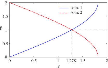
Figure 1: The two solutions obtained for $0<\beta<2$ for different values of $q\in\left(0,1.816\right)$. We use the solid curve in our analysis.

Proceeding as described above, we vary $q$ between 0 to 1.816. For each $q$, we obtain multiple roots. The non-uniqueness in $\beta$ can be understood by examining Eqs. (11) through (13), with $N=\infty$. In such a case, clearly any $\beta$ can be replaced by $\pm\beta+2k$ for any integer $k$. For this reason, we restrict attention to $0<\beta<2$. Even this restricted case has two solutions for any $q$. These two solutions for different $q$ are shown in Fig. 1. The solution curves cross at $q\approx 1.278$, when $\beta=1$. We use the $\beta$ corresponding to the solid line in the figure for definiteness. It turns out that the coefficients $C_{m}=D_{n}$. Finally, $\phi_{1}$ is determined by inserting $\beta=0$ for all $q$. It is found that the sines give an identically zero solution; and the cosines give the third and final linearly independent nontrivial solution. The coefficients $B_{k}$ are found without ambiguity, again with $B_{0}=1$. In the next section, we consider the collisional case, $0<\epsilon\ll 1$, and analyze the equations using the method of averaging.

IV Averaging of the collisional equations, $\mathbf{0<\epsilon\ll 1}$

We adopt the method of averaging to study Eq. (8) for $0<\epsilon\ll 1$. In order to carry out averaging, the equations need to be represented in the Lagrange standard form Verhulst , which is

$$\dot{h}=\epsilon g({h},t)+{\cal O}\left(\epsilon^{2}\right).$$ (14)

In the above, $h$ is a vector of unknowns, and the $t$-dependence of $g$ is typically oscillatory although not necessarily perfectly periodic. Note that the right-hand side is ${\cal O}\left(\epsilon\right)$. The slow flow equations are

$$\dot{h}_{{\rm av}}=\epsilon\bar{g}$$

where

$$\bar{g}=\lim_{T\to\infty}\frac{1}{T}\int_{0}^{T}g({h_{{\rm av}}},t)dt,$$

where in the right hand side, $h_{{\rm av}}$ is treated as a constant while integrating with respect to time. The averaged dynamics of $h_{{\rm av}}$ approximates the original $h$ over time scales of ${\cal O}\left(1\big{/}\epsilon\right)$. The averaging can be done over one period only, if $g$ is periodic in $t$; and over several discrete periods, term-wise, if $g$ is the sum of individual periodic terms with incommensurate periods; and over a long time with a limit, as indicated, in the general case. To solve Eq. (8), we drop terms of $\mathcal{O}\left(\epsilon^{2}\right)$ and higher and begin with Eq. (10), but with the $a_{i}$ now being treated as time-varying coordinates,

$$A\left(t\right)=a_{1}\left(t\right)\phi_{1}\left(t\right)+a_{2}\left(t\right)\phi_{2}\left(t\right)+a_{3}\left(t\right)\phi_{3}\left(t\right).$$ (15)

Differentiating the above once with respect to time, we obtain

$$\dot{A}=\dot{a}_{1}\phi_{1}+\dot{a}_{2}\phi_{2}+\dot{a}_{3}\phi_{3}+a_{1}\dot{\phi}_{1}+a_{2}\dot{\phi}_{2}+a_{3}\dot{\phi}_{3}.$$ (16)

Here, noting that we have three $a_{i}$ in place of one original unknown $A$, we must adopt two constraint equations. The choice of these constraint equations is classical and routine, and is given by

$$\dot{a}_{1}\phi_{1}+\dot{a}_{2}\phi_{2}+\dot{a}_{3}\phi_{3} =0$$

$$\dot{a}_{1}\dot{\phi}_{1}+\dot{a}_{2}\dot{\phi}_{2}+\dot{a}_{3}\dot{\phi}_{3} =0$$ (17)

which results in the following equations for the first and second derivatives of $A$,

$$\dot{A} =a_{1}\dot{\phi}_{1}+a_{2}\dot{\phi}_{2}+a_{3}\dot{\phi}_{3}$$

$$\ddot{A} =a_{1}\ddot{\phi}_{1}+a_{2}\ddot{\phi}_{2}+a_{3}\ddot{\phi}_{3}$$

Note that since $\phi_{i}$ is a solution of the $\epsilon=0$ system, it satisfies

$$a_{i}\left(\dddot{\phi}_{i}+4f\dot{\phi}_{i}+2\dot{f}\phi_{i}\right)=0,$$

identically for each $i$, and for any value of $a_{i}$, irrespective of whether $a_{i}$ is time varying or not.

We next substitute Eq. (15) in Eq. (8), and use Eq. (17), to obtain

$$\dot{a}_{1}\ddot{\phi}_{1}+\dot{a}_{2}\ddot{\phi}_{2}+\dot{a}_{3}\ddot{\phi}_{3}=-\epsilon w$$ (18)

where

$$w = -\Big{\{}12\left(a_{1}\ddot{\phi}_{1}+a_{2}\ddot{\phi}_{2}+a_{3}\ddot{\phi}_{3}\right)\left(a_{1}\phi_{1}+a_{2}\phi_{2}+a_{3}\phi_{3}\right)$$ (19)

$$+14\dot{f}\left(a_{1}\dot{\phi}_{1}+a_{2}\dot{\phi}_{2}+a_{3}\dot{\phi}_{3}\right)^{2}$$

$$-3\left(a_{1}\ddot{\phi}_{1}+a_{2}\ddot{\phi}_{2}+a_{3}\ddot{\phi}_{3}\right)-4f\left(a_{1}\phi_{1}+a_{2}\phi_{2}+a_{3}\right)$$

$$+8f\left(a_{1}\phi_{1}+a_{2}\phi_{2}+a_{3}\phi_{3}\right)^{2}\phi_{3}\Big{\}}.$$

Combining Eqs.  (17) and (18), we obtain

$$\begin{bmatrix}\phi_{1}&\phi_{2}&\phi_{3}\\ \dot{\phi}_{1}&\dot{\phi}_{2}&\dot{\phi}_{3}\\ \ddot{\phi}_{1}&\ddot{\phi}_{2}&\ddot{\phi}_{3}\end{bmatrix}\begin{Bmatrix}\dot{a}_{1}\\ \dot{a}_{2}\\ \dot{a}_{3}\end{Bmatrix}=\begin{Bmatrix}0\\ 0\\ -\epsilon w\end{Bmatrix},$$ (20)

which can be written as

$$\begin{Bmatrix}\dot{a}_{1}\\ \dot{a}_{2}\\ \dot{a}_{3}\end{Bmatrix}=-\frac{\epsilon}{\Delta}\begin{Bmatrix}\left(\phi_{2}\dot{\phi}_{3}-\phi_{3}\dot{\phi}_{2}\right)w\\ \left(\phi_{3}\dot{\phi}_{1}-\phi_{1}\dot{\phi}_{3}\right)w\\ \left(\phi_{1}\dot{\phi}_{2}-\phi_{2}\dot{\phi}_{1}\right)w\end{Bmatrix},$$ (21)

where $\Delta$ denotes the determinant of the coefficient matrix on the left hand side of Eq. (20). Conveniently, although this determinant depends on $q$, it is time-invariant for this problem, and can be calculated at $t=0$ using the computed $\phi_{i}(t)$ and their derivatives. Equation (21) is in the Lagrange standard form, and can be averaged. Fortunately and interestingly, some big simplifications are possible.

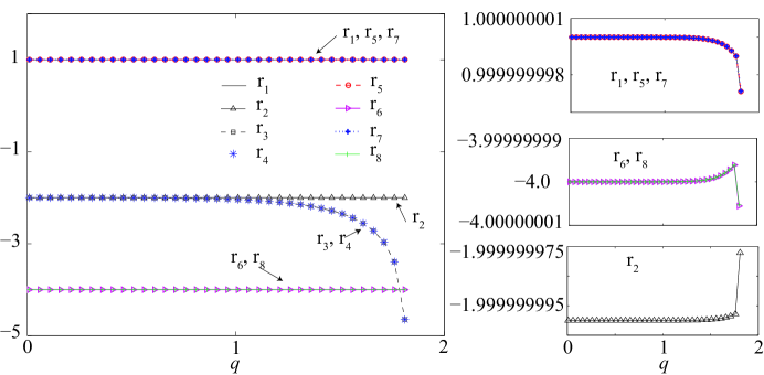
Figure 2: The numerically evaluated coefficients $r_{i}(q)$ of Eq. (22) fo various values of $q\in\left(0,1.816\right)$. Here, we have used $N=8$. As can be clearly seen in the graph, $r_{1},r_{5},r_{7}\approx 1$, $r_{2}\approx-2$, $r_{6},r_{8}\approx-4$ and $r_{3}=r_{4}\in\left(-5,-2\right)$. This finally gives the simplified slow-flow equations given by Eq. (23). The subplot on the right support our conclusion that, except for $r_{3}$ and $r_{4}$, the other coefficients are in fact integers and larger $N$ lowers the deviation from integer values.

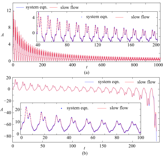
Figure 3: Comparison of the solutions obtained by direct numerical integration of Eq. (8) and numerical integration of the slow-flow equations, Eq. (23). Parameters used: $\beta=1\big{/}2$, $q=0.6899$ and $\epsilon=0.001$. The upper graph (a) depicts an asymptotically stable trajectory and the lower graph (b) an unstable one.

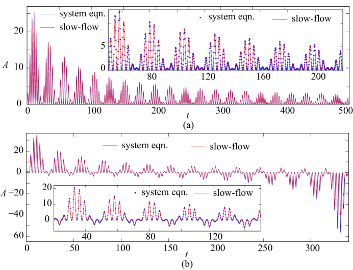
Figure 4: Comparison of the solutions obtained by direct numerical integration of Eq. (8) and numerical integration of the slow-flow equations, Eq. (23). Parameters used: $\beta=\sqrt{3}$, $q=1.775$ and $\epsilon=0.001$. The upper graph (a) depicts an asymptotically stable trajectory and the lower graph (b) an unstable one.

There are many terms in Eq. (21), and each of those terms is a product of a few functions, and each function is expanded in a series. However, using various symmetry arguments and trigonometric identities and simplifications, we can theoretically show that many of the terms above must have average values equal to zero. This is a tedious step, and details are omitted. After such simplification, a fairly large number of terms still remain, and they can be averaged either numerically, or using symbolic algebra (MAPLE), with numerical values of the coefficients $B_{k}$, $C_{m}$ and $D_{n}$ along with $\beta$, determined separately for each $q$.

After such simplification and averaging, including therein division by $\Delta$, which is constant with respect to time but depends on $q$, the remaining non-zero averages yield a final slow flow of the form

$$\dot{a}_{1} = \epsilon\left\{r_{1}(q)\,a_{{1}}+r_{2}(q)\,{a_{{1}}}^{2}+r_{3}(q)\,{a_{{2}}}^{2}+r_{4}(q)\,{a_{{3}}}^{2}\right\},$$

$$\dot{a}_{2} = \epsilon\left\{r_{5}(q)\,a_{{2}}+r_{6}(q)\,a_{{1}}a_{{2}}\right\},$$

$$\dot{a}_{3} = \epsilon\left\{r_{7}(q)\,a_{{3}}+r_{8}(q)\,a_{{1}}a_{{3}}\right\},$$ (22)

where we see that several possible quadratic terms have dropped out. Interestingly, most of the $r_{i}(q)$ in the above equation apparently have integer values if $N$ is large enough, independent of $q$ (or $\beta$)! The integer nature of these coefficients is hidden by the complex expressions involved, but the numerical evidence seems beyond the realm of coincidence. In Fig. 2, several of the coefficients are seen to be extremely close to integer values. We henceforth take these averaged coefficients as integers. There remains only one non-integer averaged coefficient, henceforth denoted by $\mu(q)$, which takes values between $2$ and $5$ approximately, and which appears twice in the slow flow, as $r_{3}(q)$ and $r_{4}(q)$. The final slow flow has a simple form:

$$\dot{a}_{1} = \epsilon\left(a_{{1}}-2{a_{{1}}}^{2}-\mu(q)\,{a_{{3}}}^{2}-\mu(q)\,{a_{{2}}}^{2}\right)$$

$$\dot{a}_{2} = \epsilon\left(a_{{2}}-4a_{{1}}a_{{2}}\right)$$

$$\dot{a}_{3} = \epsilon\left(a_{{3}}-4a_{{1}}a_{{3}}\right).$$ (23)

We now validate the averaging calculation by comparing two solutions: (i) direct numerical integration of the original, Eq. (8); and (ii) numerical integration of the slow-flow equations given by Eq. (23), followed by inserting the $a_{i}$ in Eq. (15). Figure 3 shows the solutions thus obtained for $q=0.6899$, $\beta=1\big{/}2$, $\epsilon=0.001$, $N=5$, and $\mu(0.6899)=2.008$. The upper subplot shows a bounded solution; and the lower subplot, with different initial conditions, shows an unbounded solution. Both solutions are actually plotted using two curves, one from the original equations and one from the slow flow. A zoomed view of a portion is also shown to display the excellent match between the two solutions, for small $\epsilon$. Figure 4 shows a similar match for $\beta=\sqrt{3}$ with $q=1.775$, $\epsilon=0.001$, $N=5$, and $\mu(1.775)=3.595$. The match, again, is excellent. Note that the waveforms are different in Figs. 3 and 4 because of differences in the $\phi_{i}$, although the slow flow in terms of coordinates $a_{i}$ is almost the same. Having established that the slow flow equations given by Eq. (23) do indeed capture the dynamics of the original system very well, we now proceed to study the slow flow equations themselves in the next section. They allow further simplification.

V Dynamics of the slow flow equations

Writing $\tau=\epsilon t$ (a slow time), we can remove $\epsilon$ from explicit consideration. We multiply the equation for $\dot{a}_{2}$ in Eq. (23) by $a_{2}$ and that for $\dot{a}_{3}$ by $a_{3}$, and add them to obtain

$$\frac{d}{d\tau}\left(\frac{a_{2}^{2}}{2}+\frac{a_{3}^{2}}{2}\right) = \left(a_{2}^{2}+a_{3}^{2}\right)\left(1-4a_{1}\right).$$ (24)

Writing $Z=\mu\left(q\right)\left(a_{2}^{2}+a_{3}^{2}\right)$, where $Z\geq 0$, we find that Eq. (23) collapse to a two dimensional parameter-free form,

$$\dot{a}_{1} = -Z+a_{1}\left(1-2a_{1}\right),$$ (25)

$$\dot{Z} = 2Z\left(1-4a_{1}\right),$$ (26)

where the overdots denote derivatives with respect to $\tau=\epsilon t$. Eqs. (25) and (26) have a single, simple, averaged form that characterizes the dynamics of the original Eq. (7) for small $\epsilon$. The actual value of $\mu$, and hence $q$, has no effect on the qualitative dynamics. The averaged slow flow equation, after this simple transformation, is the same for all $q$ values.

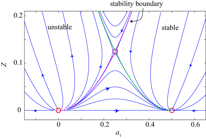
Figure 5: Unified phase portrait of Eqs. (25) and (26) in the reduced $a_{1}$-$Z$ plane with $Z\geq 0$. The fixed points (red circles) are: (i) (0,0), unstable, (0.5,0) stable, and (iii) (0.25,0.125), saddle. The dashed curve in magenta, $Z=2a_{1}^{2}$, denotes the stability boundary.

Fixed points of Eqs. (25) and (26) are easy to find. There are three of them: (i) $\left(a_{1},Z\right)=(0,0)$, unstable node, (ii) ${\displaystyle\left(0.5,0\right)}$, stable node, and (iii) ${\displaystyle\left(0.25,0.125\right)}$, saddle. Figure 5 shows the phase portrait for Eqs. (25) and (26) and for $Z\geq 0$. The circles therein denote the fixed points. The blue lines denote numerically integrated solutions. The dashed lines denote two invariant manifolds. These invariant manifolds are parabolas. To obtain one of them, assume $Z=ka_{1}^{2}$. For this parabola to be an invariant manifold, all points on it must have $\dot{Z}$ and $\dot{a}_{1}$ in the proportion $2ka_{1}$. It is easy to check that this condition is satisfied for $k=2$. The other invariant manifold, a shifted parabola, is similarly found. In the phase portrait of Fig. 5, the dashed curve in magenta, $Z=2a_{1}^{2}$, is the stability boundary. Solutions that originate on right of the boundary are stable, while those on the left are unbounded. All stable solutions settle on $a_{1}=0.5$, and $Z=0$ or $a_{2}=a_{3}=0$. As $A=\sum_{i}a_{i}\phi_{i}$ (recall Eq. (15)), this means that solutions of the original system, Eq. (7), either grow without bound, or settle to $\pi$-periodic oscillations (corresponding to a purely $\phi_{1}$ solution). This conclusion holds for all $0<q<1.816$.

VI Discussion and conclusions

In this paper, we have analyzed the Fokker-Planck equation for a plasma in a Paul trap and found that the averaged equations satisfy the dynamical behavior shown in Fig. 5 irrespective of the value of the parameter $q\in\left(0,1.816\right)$. This is a significant result since it is usually possible to analyze the plasma distribution function only for small values of the system parameters Dutta ; Shah2008 . Out of all the possible averaged solutions corresponding to different initial values of $a_{1}$ and $Z$ in Fig. 5, determining which ones are physically meaningful requires considerable further analysis since the functions $A,B$ and $C$ have to be analyzed for all $q$, different initial conditions in a three-dimensional space and as a function of time. However, the important point to note here is that, in any case, the form of the solution we have chosen in Eq. (6) admits only one unique stable time-periodic solution. Hence, irrespective of their initial values and/or parameter $q$, the actual time-varying functions $A,B$ and $C$ can asymptotically either reach the unique stable time-periodic solution or diverge to infinity. This result holds true for all values of $q\in\left(0,1.816\right)$. We have checked that for the stable time-periodic solution at $a_{1}=0.5$ and $Z=0$ as shown in Fig. 5, the corresponding initial conditions satisfy $A>0$, $C>0$ and $4AC-B^{2}>0$, which shows the existence of a normalizable initial distribution corresponding to this solution. This implies that the initial distribution in a small neighborhood around this time-periodic solution will also be normalizable and asymptotically reach this same stable solution.

One may ask what happens to the solutions if we chose a form different from that given in Eq. (6). The question is not easy to answer, because any such assumed form leads to new equations, and new constraints which must be checked. The area is certainly promising for future research. However, for the case of a spatially linear electric field, the resulting solutions are likely to be qualitatively similar to that obtained in this paper. Namely, a set of initial conditions will perhaps converge to the same stable time-periodic solution given in this paper and another set of initial conditions will lead to divergent solutions.

A more important question is, what happens if the trapping field itself is nonlinear? In such cases, the entire approach will require rethinking. The lack of an underlying linear system will make superposition impossible; the possibility of amplitude-dependent solution frequencies will make resonances more complex and numerous; and the dynamics of even a single ion will involve significant challenges. In such a situation, the dynamics of a cloud of ions may well exhibit new and complex phenomena quite different from the remarkably simple unifying dynamics that has been discovered in this paper ShahPhD .

- (1) M. M. Turner, “Pressure Heating of Electrons in Capacitively Coupled rf Discharges”, Phys. Rev. Lett. 75, 1312 (1995)
- (2) W. Paul, “Electromagnetic traps for charged and neutral particles”, Rev. Mod. Phys. 62, 531 (1990)
- (3) K. Shah and H. S. Ramachandran, “Analytic, nonlinearly exact solutions of an rf confined plasma”, Phys. Plasmas 15, 062303 (2008)
- (4) L. Corte, P. M. Chaikin, J. P. Gollub and D. J. Pine, “Random organization in periodically driven systems”, Nature Physics 4, 420–424 (2008)
- (5) V. N. Smelyanskiy, M. I. Dykman and B. Golding, “Time oscillations of escape rates in periodically driven systems”, Phys. Rev. Lett. 82, 3193 (1999)
- (6) K. Shah, D. Turaev, V. Gelfreich and V. Rom-Kedar, “Equilibration of energy in slow-fast systems”, Proc. Natl. Acad. Sci. USA 114, E10514 (2017)
- (7) S. Rahav, I. Gilary, and S. Fishman, “Effective Hamiltonians for periodically driven systems”, Phys. Rev. A 68, 013820 (2003)
- (8) V. Gelfreich, V. Rom-Kedar and D. Turaev, “Fermi acceleration and adiabatic invariants for non-autonomous billiards”, Chaos 22, 033116 (2012)
- (9) A. I. Neishtadt and Y. G. Sinai, “Adiabatic piston as a dynamical system”, J. Stat. Phys. 116, 815 (2004)
- (10) V. L. Ryjkov, X. Z. Zhao and H. A. Schuessler, “Simulations of the rf heating rates in a linear quadrupole ion trap”, Phys. Rev. A 71, 033414 (2005)
- (11) L. Deslauriers, S. Olmschenk, D. Stick, W. K. Hensinger, J. Sterk and C. Monroe, “Scaling and Suppression of Anomalous Heating in Ion Traps”, Phys. Rev. Lett. 97, 103007 (2006)
- (12) V. Saxena and K. Shah, “Time evolution of Tsallis distribution in Paul trap”, IEEE Trans. Plasma Science 45, 918 (2017)
- (13) G. T. Abraham, A. Chatterjee and A. G. Menon, “Escape velocity and resonant ion dynamics in Paul trap mass spectrometers”, Int. J. Mass Spect. 231, 1 (2004)
- (14) N. W. McLachlan, Theory and Applications of Mathieu Functions (Oxford University Press, Oxford, 1947)
- (15) D. R. Nicholson, Introduction to Plasma Theory (Wiley, New York, 1983)
- (16) K. Shah and H. S. Ramachandran, “Space charge effects in rf traps: Ponderomotive concept and stroboscopic analysis”, Phys. Plasmas 16, 062307 (2009)
- (17) S. Banerjee and K. Shah, “Vlasov dynamics of periodically driven systems”, Phys. Plasmas 25, 042302 (2018)
- (18) H. Risken, The Fokker–Planck Equation: Methods of Solutions and Applications (Springer, Berlin, 1989)
- (19) S. Chandrasekhar, “Stochastic problems in physics and astronomy”, Rev. Mod. Phys. 15, 1 (1943)
- (20) S. B. Dutta and M. Barma, “Asymptotic distributions of periodically driven stochastic systems”, Phys. Rev. E 67, 061111 (2003)
- (21) K. Shah, “Asymptotic solution of Fokker–Planck equation for plasma in Paul traps”, Phys. Plasmas 17, 054501 (2010)
- (22) F. Verhulst, Nonlinear differential equations and dynamical systems (Springer, Berlin, 2006)
- (23) K. Shah, “Plasma dynamics in paul traps”, Ph.D dissertation, Dept. Elect. Eng., Indian Institue Technology Madras, India, Mar. 2010