Abstract

Submillimeter emission lines of carbon monoxide (CO) in Titan’s atmosphere provide excellent probes of atmospheric temperature due to the molecule’s long chemical lifetime and stable, well constrained volume mixing ratio. Here we present the analysis of 4 datasets obtained with the Atacama Large Millimeter/Submillimeter Array (ALMA) in 2012, 2013, 2014, and 2015 that contain strong CO rotational transitions. Utilizing ALMA’s high spatial resolution in the 2012, 2014, and 2015 observations, we extract spectra from 3 separate regions on Titan’s disk using datasets with beam sizes ranging from $0.35\times 0.28^{\prime\prime}$ to $0.39\times 0.34^{\prime\prime}$. Temperature profiles retrieved by the NEMESIS radiative transfer code are compared to Cassini Composite Infrared Spectrometer (CIRS) and radio occultation science results from similar latitude regions. Disk-averaged temperature profiles stay relatively constant from year to year, while small seasonal variations in atmospheric temperature are present from 2012–2015 in the stratosphere and mesosphere ($\sim$100-500 km) of spatially resolved regions. We measure the stratopause (320 km) to increase in temperature by 5 K in northern latitudes from 2012–2015, while temperatures rise throughout the stratosphere at lower latitudes. We observe generally cooler temperatures in the lower stratosphere ($\sim$100 km) than those obtained through Cassini radio occultation measurements, with the notable exception of warming in the northern latitudes and the absence of previous instabilities; both of these results are indicators that Titan’s lower atmosphere responds to seasonal effects, particularly at higher latitudes. While retrieved temperature profiles cover a range of latitudes in these observations, deviations from CIRS nadir maps and radio occultation measurements convolved with the ALMA beam-footprint are not found to be statistically significant, and discrepancies are often found to be less than 5 K throughout the atmosphere. ALMA’s excellent sensitivity in the lower stratosphere (60–300 km) provides a highly complementary dataset to contemporary CIRS and radio science observations, including altitude regions where both of those measurement sets contain large uncertainties. The demonstrated utility of CO emission lines in the submillimeter as a tracer of Titan’s atmospheric temperature lays the groundwork for future studies of other molecular species – particularly those that exhibit strong polar abundance enhancements or are pressure-broadened in the lower atmosphere, as temperature profiles are found to consistently vary with latitude in all three years by up to 15 K.

1 Introduction

Titan’s atmospheric temperature, strongly influenced by solar heating, photochemistry, cloud and haze formation, and Hadley-type circulation, has been shown to have large spatial and temporal variations in the lower and middle atmosphere ($\leq$600 km). Many measurements of Titan’s atmospheric temperature and dynamics have been made in the previous decades from ground- and space-based facilities, including the Submillimeter Array, Voyager 1, and Cassini orbiter observations, through radio occultations, ultraviolet, infrared, near-IR, heterodyne, and submillimeter spectroscopy (see reviews in [19], and [21]). The Cassini spacecraft, in particular, has provided unprecedented measurements of atmospheric temperature in Titan’s troposphere and stratosphere through modeling CH₄ vibrational-rotational emission in the IR and in situ measurements by the Huygens Atmospheric Structure Instrument (HASI) [20, 18, 48, 16, 1, 42, 43, 2, 44, 49, 14]. Additionally, temperatures in the lower atmosphere have been obtained through Cassini radio occultations, where spacecraft signals are refracted by Titan’s atmosphere during transmission to Earth [39, 40]. These datasets have constrained temperatures to $\leq$1 K over many close flybys of Titan starting in 2004. Throughout Cassini’s extended tour of the Saturnian system, close to half of a full seasonal cycle (29.5 years) has been observed on Titan; however, Cassini’s finale in 2017 will greatly limit further studies of Titan’s atmosphere with such exceptional resolution and cadence.

In addition to commonly used atmospheric temperature diagnostics such as thermal emission and modeling CH₄ bands in the IR – whose abundance is well constrained in Titan’s atmosphere by Cassini and in situ measurements by the Huygens probe [33] – CO may also be used as a probe for atmospheric temperature. Previous observations of Titan in the IR and submillimeter regimes from ground- and space-based facilities on Earth have provided many constraints on CO abundance throughout the atmosphere by utilizing a priori temperature measurements from Cassini and Voyager 1 observations [23, 28, 22, 36, 13, 24, 15, 45, 37]. The volume mixing ratio of CO, found to be approximately 50 ppm, appears to be extremely stable throughout Titan’s atmosphere as found by observations and photochemical models due to its long photochemical lifetime, estimated to be upwards of 75 Myr [50, 23, 28, 26, 29]. [41] recently retrieved disk-averaged temperature profiles by modeling CO emission lines present in flux calibration images of Titan obtained with the Atacama Large Millimeter/Submillimeter Array (ALMA) during 2012 and 2014, and determined a constant CO volume mixing ratio of 49.6 ppm.

Here we present the first spatially resolved temperature measurements of Titan obtained using ground-based radio observations. We analyze data from four short ($\sim$3 minute) ALMA flux calibration observations of Titan to obtain disk-averaged measurements in atmospheric temperature from 2012–2015, and independent temperature measurements of three distinct latitude regions ($\sim 48^{\circ}$ N, $20^{\circ}$ N, and $15^{\circ}$ S) in 2012, 2014, and 2015. We compare temperature profiles covering altitudes in Titan’s lower stratosphere through mesosphere (50–500 km) to those obtained by Cassini Composite Infrared Spectrometer (CIRS) nadir mapping observations and through radio occultations. Through the future combination of ALMA and Cassini datasets, this technique may be used to monitor Titan’s atmospheric temperature and dynamics into northern summer, completing the seasonal cycle observed by Cassini beginning in northern winter in 2004.

2 Observations

We obtained public data of Titan from the ALMA science archive. Titan is often used as a flux calibrator for ALMA science targets, allowing us to utilize frequent (almost daily for $\sim$7 months of the year) observations over the duration of ALMA’s lifespan for this study. Though many additional datasets containing short integration times on Titan exist in the ALMA science archive, we employed only those observations with beam sizes roughly one third of Titan’s angular diameter – $\sim$1^′′ including the moon’s solid body and atmosphere. During early cycles, the spatial resolution was often >$0.20^{\prime\prime}$ due to fewer available antennae in the array. High spatial resolution data from 2013 are particularly limited, as the ALMA array was undergoing construction and commissioning during this period, resulting in few useful observations. Observational parameters are given in Table LABEL:tab:obs for the datasets used in this study.

We completed data reduction in a fashion similar to previous ALMA studies of Titan [11, 12, 41, 30, 35]. We processed data using modified versions of the scripts provided by the Joint ALMA Observatory, which often flag out strong lines in Titan’s atmosphere (such as CO). We re-ran these scripts in the NRAO’s CASA software package 4.7.0 to correctly include CO lines, and executed standard protocols such as flagging terrestrial lines and shadowed data, bandpass and gain calibration. Imaging was completed using the CASA clean task. Deconvolution of the ALMA point-spread function was performed by using the Högbom algorithm, with natural visibility weighting and an flux threshold of twice the expected RMS noise (typically on order 15 mJy). The image pixel sizes were set to 0.03${}^{\prime\prime}\times$0.03^′′. Image spectral coordinates were Doppler-shifted to Titan’s rest frame using Topocentric radial velocities from JPL Horizons ephemerides.

We obtained disk-averaged measurements for each year from 2012–2015 by extracting flux over Titan’s solid disk (2575 km), plus its extended atmosphere (1200 km) and an additional 2-$\sigma_{PSF}$, where $\sigma_{PSF}$ is the standard deviation of ALMA’s point-spread function, or the FWHM (major axis) of the Gaussian restoring beam. ALMA configurations in 2012, 2014, and 2015 permitted beam sizes that are smaller than Titan’s angular diameter, allowing us to extract independent flux measurements of multiple, spatially resolved regions on Titan’s disk. We chose to model spectra from 3 regions (hereafter referred to as ‘North’, ‘Center’, and ‘South’) chosen to be as independent as possible (with minimal beam overlap), while the mean latitudes of extraction regions are within $5^{\circ}$ from year to year. These regions are shown in Fig. 1. As such, flux density measurements from these “beam-footprints” are representative of a few latitude decades.

We obtained initial flux density estimates by using the Butler-JPL-Horizons 2012 Titan flux model in the CASA reduction scripts, which is expected to be accurate to within 5$\%$ (see ALMA Memo $\#$594). This model is based on previous ground-based submillimeter observations of Titan, and includes: strong emission lines from trace species in Titan’s atmosphere – namely CO, HCN, and their respective isotopologues; collisionally-induced absorption of N₂-N₂ and N₂-CH₄; emission from Titan’s surface [23, 22].

3 Spectral Modeling and Results

We converted ALMA spectra to spectral radiance units (nW/cm²/sr/cm^-1) as described by [45] before performing radiative transfer modeling using the Non-Linear Optimal Estimator for Multivariate Spectral Analysis (NEMESIS) software package in line-by-line mode [25]. We obtained spectral line parameters from the HITRAN 2012 and CDMS databases [38, 31] as in [41, 30]. We calculated collisionally-induced absorption parameters for N₂, CH₄, and H₂ pairs from the works of Borysow and Frommhold [*]borysow_86a,borysow_86b, borysow_86c, borysow_87, Borysow [*]borysow_91, and Borysow and Tang [*]borysow_93. We then initialized models of Titan’s atmosphere using N₂ and CH₄ vertical profiles from [34] and [45], with a constant CO abundance of 49.6 ppm as found by [41], which is in agreement with previous CO measurements [16, 43, 24, 15, 45, 37]. Assuming the CO abundance profile is constant due to its long photochemical lifetime allows us to fit spectra by only varying vertical temperature profiles, as emission lines of CO are significantly pressure-broadened in Titan’s atmosphere and thus enable temperature retrievals from a wide range of altitudes. Temperature retrievals obtained using CO abundances in excess of ±$20\%$ of the nominal value (49.6 ppm) resulted in poor spectral fits or large variations in temperature, as in [41]. Using a non-uniform CO abundance profile with small variations (<5 ppm), such as that found by [29], has little effect on spectral fits and retrieved temperature profiles.

We first model disk-averaged spectra to obtain initial temperature profiles for each dataset listed in Table LABEL:tab:obs. As emission from Titan’s extended atmosphere results in significant limb brightening, we generated spectral models using 37–44 field-of-view averaging points (available online from [Dataset] [46]), as detailed in Appendix A of [45]. As a starting point for our disk-averaged retrievals, we constructed a priori temperature profiles using data constrained by measurements from Cassini CIRS and the Huygens probe [18, 20], as in previous ALMA studies of Titan [11, 12, 41, 30]. Additionally, we also use contemporary disk-averaged CIRS nadir data (similar to [3]), which provide high sensitivity measurements between 0.1–10 mbar. These datasets are detailed in Table LABEL:tab:cassini. Upper atmospheric temperatures (>600 km) were held as isothermal at 160 K.

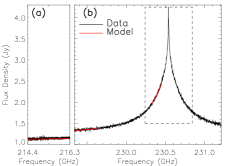
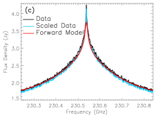
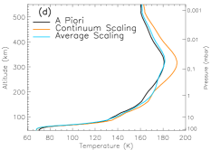
Figure 2: (a, b) ALMA spectra (black) from adjacent continuum (a) and CO (2-1) line (b) spectral windows from ALMA dataset 2012.1.00317.S (Table LABEL:tab:obs). Synthetic spectra (red) show regions modeled to determine uniform offsets between data and models. The boxed region denotes the spectral range chosen to model for temperature retrievals. (c) Close up of boxed region in (b). ALMA data (black) is compared to data scaled by a constant factor (0.974; teal) obtained by averaging offsets of regions shown in (a, b). NEMESIS synthetic spectrum is shown before temperature retrieval (red). (d) Temperature retrievals for data scaled by the continuum scaling factor (0.990; orange) from (a), and average factor (0.974; teal) as shown in (c). The a priori temperature profile is plotted in black.

Initial fits of continuum regions in adjacent spectral windows were greatly improved by utilizing temperature profiles of Titan’s lower atmosphere obtained by Cassini radio occultation science ([40]; Table LABEL:tab:cassini). While these observations are not contemporary with those by ALMA, temperatures near Titan’s tropopause (40–60 km, where the radio continuum is formed) are not expected to change on seasonal timescales, but do vary with latitude [17, 40]. We then multiplied our spectra by a small scaling factor (<5$\%$ of the spectral radiance) due to discrepancies between our model and that of Butler-JPL-Horizons 2012. These discrepancies may be due to: slight latitudinal troposphere temperature variations (on the order 5 K) between the models; minor uncertainties in line broadening or collisionally-induced absorption parameters; and variations in CO abundance on the order of 10$\%$. A constant scaling factor was determined for each spectrum by averaging offsets between measurements of data and model continuum, CO line wings, and line core regions, to distinguish between minute flux calibration issues during the ALMA pipeline and effects caused by temperature variations in Titan’s atmosphere. Synthetic spectra generated to determine scaling factors for the 2015 CO (2–1) line, along with a comparison of the CO line forward model, unscaled, and scaled data are shown in Fig. 2 (panels a, b, and c). The effects of these scaling factors on the retrieved temperature profiles are shown in Fig. 2d.

We retrieve vertical temperature profiles by allowing NEMESIS to vary temperature measurements continuously throughout the atmosphere, with 5 K errors set on the a priori temperature profile; combined with a correlation length of 1.5 scale heights, these errors enable NEMESIS to adjust temperature profiles enough to obtain excellent spectral fits, but reduce ill-conditioning (artificial vertical structure; [25]). We assume that small scale vertical structure is a result of NEMESIS fitting noise in the spectrum, and is not a result of atmospheric dynamics (e.g. gravity waves) – these correlation length and a priori errors are large enough to properly constrain the spectral fit, but provide sufficient smoothing to prevent unrealistic vertical oscillations.

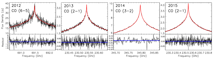
Figure 3: ALMA spectra (black) and synthetic spectra generated by the NEMESIS radiative transfer code (red) for disk-averaged measurements of flux from 2012–2015 datasets. Bottom panels show the residual flux after subtracting the model from the observed spectrum.

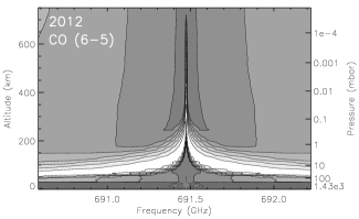
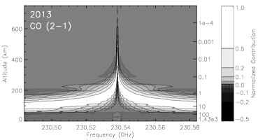
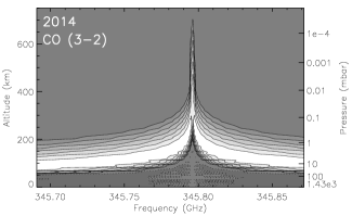
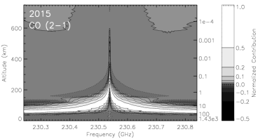
Figure 4: Contours of normalized functional derivatives [25] of spectral radiance per wavenumber with respect to temperature for each disk-averaged spectrum in Fig. 3. Contour levels are 0, ±0.0046, ±0.01, ±0.0215, ±0.046, ±0.1, ±0.215, and ±0.46, as in [30]; levels express CO emission sensitivity to temperature at various pressure and altitude values.

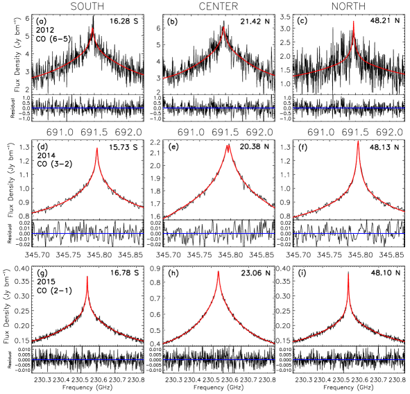
Figure 5: ALMA spectra (black) and synthetic spectra generated by the NEMESIS radiative transfer code (red) for spatially resolved datasets from 2012 (a–c), 2014 (d–f), and 2015 (g–i). Mean latitudes for beam-footprint regions are shown, which correspond to regions in Fig. 1. Bottom panels show the residual flux as in Fig. 3.

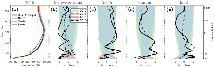
Figure 6: (a) Retrieved temperature profiles for 2012 disk-averaged (black line) and spatial spectra (blue, green, and red) fit by the NEMESIS radiative transfer code shown in Fig. 3 and 5, respectively. The 1-$\sigma$ error envelope of the disk-averaged retrieval is shown in gray. Temperature profiles are plotted where the CO retrievals are most sensitive, as shown in Fig. 4. (b) Comparison of temperature difference in disk-averaged profiles from 2013 (dash dot), 2014 (solid), and 2015 (dashed) with respect to 2012 from panel a. Error envelopes for 2012, 2013, 2014, and 2015 datasets are shown (green, purple, red, and blue, respectively). (c–e) Variations in spatial profiles for 2014 and 2015 data compared to the 2012 profiles from panel a; 2012, 2014, and 2015 error envelopes are shown.

The resulting disk-averaged synthetic spectra are shown in Fig. 3. Though our model atmosphere extends from 0–1200 km, we found the temperature sensitivity of our observations to be greatest between $\sim 10^{2}-10^{-3}$ mbar (approximately 50–530 km), as shown by contribution functions in Fig. 4. We proceeded to use disk-averaged measurements as a priori temperature profiles to model spatially resolved spectra, enabling spatial temperature profiles to be retrieved without the use of corresponding Cassini data in the stratosphere through mesosphere. For the 2014 and 2015 datasets, Cassini radio science and HASI data were convolved with the ALMA restoring beam (in the locations specified in Fig. 1) to produce interpolated temperature profiles for use as a priori values in Titan’s troposphere. This resulted in better fits to the continuum and ensured that flux density scaling factors were within the errors of the Butler-JPL-Horizons 2012 model for CO lines. Spatial spectral models are shown in Fig. 5. Finally, the retrieved 2012 disk-averaged and spatial temperature profiles are shown in Fig. 6a, with variations in 2013–2015 disk-averaged profiles shown in 6b. Deviations from 2012 spatial temperature profiles for 2014 and 2015 data are shown in Fig. 6c–e. All retrieved temperature profiles are available to download online ([Dataset] [47]).

4 Discussion

4.1 Cassini Comparisons

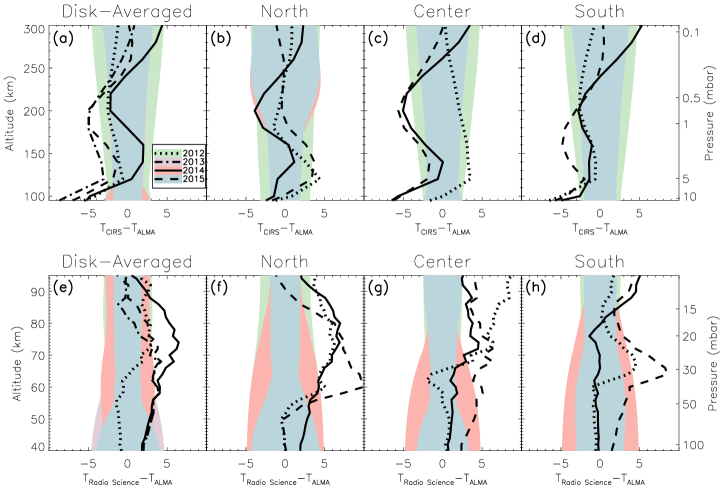
Figure 7: (a–d) Difference between CIRS nadir maps and ALMA retrievals for disk-averaged (panel a) and spatially resolved profiles (panels b–d) from 2012 (dotted lines), 2013, (dash dot), 2014 (solid), and 2015 (dashed) datasets. 1-$\sigma$ error envelopes are shown in color as in Fig. 6. CIRS nadir data were convolved with ALMA beam-footprints (Fig. 1) and are sensitive between 0.1–10 mbar ($\sim$100-300 km). (e–h) Deviations of ALMA retrievals from Cassini radio occultation science ([40]) and HASI data ([20]) interpolated at ALMA beam-footprint locations. Radio science data are accurate to within 1 K up to $\sim$10 mbar (100 km).

To validate our model of Titan’s atmosphere and the retrieved temperature profiles presented in Fig. 6, it is useful to compare these temperature measurements to those made by Cassini in similar latitude regions. Interpolating the HASI [20] and Cassini radio occultation science measurements from the T27, T31, T46, and T57 flybys [40] at the latitudes of the ALMA restoring beam (see Fig. 1) provides well constrained temperatures from 7 distinct latitude regions on Titan’s disk for altitudes 0–100 km. Though these data contain temperature measurements of Titan’s stratosphere, they are not close enough in time to warrant detailed comparisons, as stratospheric temperatures change on much shorter timescales than those in the troposphere [17, 19]. Thus, for stratospheric temperature comparisons, we elected to extract similar data from CIRS nadir maps taken during the T84, T98, T100, and T112 flybys of Titan. These maps – produced by modeling thermal infrared spectra within the P and Q branches of the $\nu_{4}$ CH₄ band (1251–1311 cm^-1), as described in detail in [1] – provide exceptional latitude coverage ($2.5^{\circ}$ resolution) over Titan’s disk during its transition into northern summer. Specific flybys were chosen to maximize latitudinal coverage from temporally comparable measurements. These flybys are listed in Table LABEL:tab:cassini, with the corresponding data available online ([Dataset] [4]). We compare these two datasets to retrieved disk-averaged and spatially resolved temperature profiles in Fig. 7.

Temperature profiles obtained from ALMA retrievals are generally in good agreement with both disk-averaged Cassini/CIRS measurements (Fig. 7a) and those from similar latitudinal regions (Fig. 7b–d). Discrepancies between CIRS and ALMA measurements in the stratosphere (100–300 km) are mostly less than 5 K. Uncertainties in our ALMA temperature retrievals range between ±2–5 K in this altitude range, while CIRS measurements are accurate to <1 K [1]. We find slightly warmer (average 1–2 K, maximum 5 K) disk-averaged stratospheric temperatures than CIRS for each year near 1 mbar (200 km), except 2014. Northern and central spatial temperature measurements for 2012 (Fig. 7b–c solid lines) are generally cooler than CIRS by up to $\sim$4 K, while southern temperatures (Fig. 7d) are comparably warmer. These variations largely lie within the retrieved temperature profile errors (Fig. 7, dark gray regions) until below 5 mbar, where CIRS profiles generally are less sensitive and relax back to a priori values. This sharp cutoff is present in all disk-averaged profiles and spatial 2014 and 2015 variations as well, resulting in 5–10 K warmer ALMA retrievals near 10 mbar. Northern and central temperature profiles from 2014 are warmer than CIRS measurements by up to 4 K between 0.5–1 mbar. Spatial retrievals of 2015 data yield the largest disparities, particularly for the southern and central regions, which were both warmer than CIRS by up to 5 K near 1 mbar.

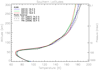
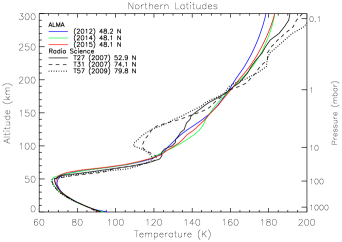
Figure 8: Comparison of spatial ALMA retrievals from 2012 (blue lines), 2014 (green), and 2015 (red) to radio occulation results ([40], Table LABEL:tab:cassini) at southern (left) and northern (right) latitudes (black lines). Radio science measurements were not convolved with ALMA beam-footprints to show seasonal variations in the lower atmosphere from 2007–2015, particularly above 100 km.

We obtain temperature profiles that are cooler than interpolated radio occultation measurements by up to 10 K for all disk-averaged and spatially resolved measurements between 50–100 km (Fig. 7e–h). At lower altitudes, ALMA retrievals are no longer sensitive to temperature (Fig. 4), and thus adhere to the a priori profile. Above 100 km, temperatures retrieved through radio occultations have uncertainties on the order 1–10 K [40], and we defer to CIRS nadir measurements which have lower errors and are from more recent Cassini observations. To illustrate the potential discrepancies between our presented ALMA retrievals and interpolated radio occultation data from 2007–2009 as a result of seasonal changes, particularly above the tropopause, we compare our retrieved temperature profiles to those published by [40] up to 300 km in Fig. 8. From 0–300 km, southern profiles generally agree with those obtained by radio occultations despite considerable latitudinal and temporal differences. However, in northern latitudes, we do not observe previous instabilities as observed by Cassini, potentially caused by cloud formation or enhanced photochemical production during northern winter [40, 19].

Most CIRS temperature variations above and below 1 mbar are within the range of ALMA retrieval errors, as are those for the radio occultation data below 30 mbar ($\sim$65 km); however, larger disparities arise for the 2014 and 2015 datasets in both the disk-averaged and spatially resolved cases than for 2012 and 2013 measurements in both regimes. This is most likely due to the vast improvement of ALMA data between 2012 and 2015 observations due to the expanded interferometer (see ‘$\#$ of Antennae’ in Table LABEL:tab:obs), resulting in increased coverage of the u-v plane and higher S/N spectra (see Fig. 3). This makes minor flux calibration issues, solved by applying a small multiplicative scaling factor (discussed in Section 3), result in greater variations between retrieved temperature profiles and Cassini measurements (see Fig. 2). Many uniform scaling factors applied to the spectral radiance (of order $\sim 5\%$) resulted in temperature retrievals with much larger deviations from Cassini data, often yielding cold (<65 K) tropopause and hot (>200 K) stratospheric temperatures. Generally, these factors are larger for high spatial resolution spectra due to the large temperature gradients that exist at high latitudes [40, 14] and are not accounted for in the flux calibration model. These systematic errors provide a motivation for improving the ALMA flux calibration model of Titan to incorporate the effects of latitudinal and seasonal variations in tropospheric and stratospheric temperatures, respectively, which can produce large uncertainties in pressure-broadened lines in Titan’s atmosphere (such as CO and HCN). For disk-averaged spectra, however, continuum measurements are close enough to our model spectra (within $\sim 2\%$) to provide a reliable calibration source for other ALMA science targets; Titan continuum windows are often used to set the flux density for science objects and spectral regions containing CO, HCN, and other strong lines on Titan itself.

Despite the aforementioned uncertainties, we find that applying a two-sample Kolmogorov-Smirnov (KS) test to the temperature profiles presented here with respect to those from Cassini/CIRS and radio occultation science reveals a high degree of correlation, and that variations – particularly those $\leq$5 K, often within the retrieved errors – are not statistically significant. These statistics are detailed in Table LABEL:tab:chisq, with the KS test statistic (D), and corresponding significance level ($\alpha$), shown for all retrieved profiles compared to Cassini/CIRS and interpolated radio occultation profiles at altitudes <100 km. Though variations in retrieved ALMA and radio science measurements do not seem statistically significant (i.e. $\alpha$>0.10), general KS significance levels are lower than for CIRS comparisons, and lower stratospheric ($\geq$60 km) temperature deviations are often larger than the retrieved error for ALMA observations (Fig. 7e–h).

4.2 Spatial and Temporal Variations

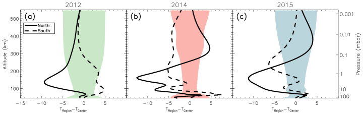
Figure 9: Year by year comparisons of differences between North (solid lines) and South (dashed) temperature profiles with temperatures extracted from Center regions. 1-$\sigma$ error envelopes for Center profiles are shown in color.

We observe little variation in disk-averaged temperature profiles from 2012–2015, as shown in Fig. 6b. These measurements agree with previous disk-averaged temperature profiles obtained with ALMA [41] and with CIRS nadir measurements (Fig. 7a), which both show small dispersion between retrieved disk-averaged temperatures. Temporal and spatial variations become apparent, however, when comparing individual regions on Titan’s disk. Variations by region are shown in Fig. 6c–e, and yearly comparisons of north and south regions to central profiles are shown in Fig. 9.

Northern regions show general warming over all three years throughout the stratosphere (particularly from 100–300 km), as the northern hemisphere receives higher insolation during the transition into northern summer. Stratopause ($\sim$310–330 km) temperatures for both 2014 and 2015 are warmer than measured in 2012 by about 5 K (Fig. 6c), in good agreement with [14]. The northern stratosphere from $\sim$80–250 km generally remains cooler than the central latitudes by 10 K (Fig. 9), consistent with CIRS limb and nadir observations throughout the Cassini mission [49, 14]. The stratopause, however, becomes warmer than central and southern profiles by 5 and 10 K, respectively, during 2014 and 2015.

Southern temperatures rise in the stratosphere from 2012–2015 by up to 5 K, particularly between 1–10 mbar, and throughout the strato- and mesosphere from 2014–2015 by a similar amount. This is explained by increased downwelling of Titan’s large Hadley-type circulation cell, which may warm the upper stratosphere and mesosphere (>300 km) of the winter pole substantially. This has been observed in both Cassini observations [44, 49] and general circulation models (GCM) of Titan [32, 27]. Southern profiles remain warmer than those at high northern latitudes throughout 2012–2015 in the lower stratosphere by 5–15 K, and cooler than the central profiles in 2014–2015 by $\sim$5 K. These results are explained by the viewing geometry of Titan as seen by ALMA, as the southern latitudes we observe are relatively low. Temperature profiles in the south will not be truly indicative of the winter pole, where the stratosphere should be quite cold [14]; indeed, deviations from the center – which is less effected by seasonal variations and reduced insolation – are much less pronounced in the south than the north. The central region follows a similar trend to the north in the lower stratosphere, though reduced in magnitude. The upper atmosphere cools in 2014 and rises again in 2015 similar to southern profiles, yet these changes are well within the retrieved errors.

We observe general cooling of the lower stratosphere ($\leq$100 km) in all three regions over 2012–2015 within the retrieved errors, with the exception of the south from 2012–2014 and the center from 2012–2015; here we observe heating above the tropopause by up to 5 K in the south and cooling by the same amount in the center (Fig. 6d–e). While seasonal changes at these altitudes are dampened compared to the stratosphere, we observe consistent latitudinal variations (Fig. 9) below 100 km as observed in Cassini radio occultation measurements [40]. Southern profiles are consistently warmer than central measurements by up to 8 K, particularly near 60 km. Northern profiles tend to match central temperatures (within the errors) at these altitudes. Considerable variability does exist, however, between northern profiles for all three years near 10 mbar (100 km), where seasonal effects may begin to manifest in atmospheric temperatures over smaller timescales. We observe the largest temporal temperature variation of all profiles presented here, 7 K, from 2012–2014 at $\sim$ 120 km (Fig. 6c), despite remaining colder than central and southern temperatures by 10–15 K (Fig. 9). However, this increase in temperature subsides from 2014–2015. While these variations are not as significant as those observed by Cassini at higher latitudes [14], this region is of particular interest for future ALMA studies. Submillimeter CO emission is particularly sensitive to temperatures at these altitudes (Fig. 4), providing insight into temperature variations below the CIRS sensitivity range and where radio science uncertainties become large. Further, these altitudes are high enough to not be significantly impacted by uncertainties in flux calibration scaling factors or models of the continuum (formed near the tropopause), which often manifest as large variations in the stratopause and tropopause (Fig. 2c).

Temperatures in the mesosphere (altitudes $\geq$ 350 km) cool in central and southern regions from 2012–2014 by up to 5 K, and rise in the north by similar amounts. However, from 2014 to 2015, these variations are often reduced substantially or reversed, as in the center and south. As the radiative dampening time of Titan’s upper atmosphere is less than a year, mesospheric temperatures become highly variable [2, 44, 19], though these results are consistent with an adiabatic cooling of the summer pole by 5 K in GCM studies [32]. This provides further motivation for increased observation of Titan with ALMA in the coming years – preferably in intervals of less than 1 year – with high spatial resolution.

While general spatial trends tend to agree with those found in GCMs and Cassini measurements, it should be noted that our temperature estimates comprise a weighted average of latitudes (see Fig. 1), and thus complex latitudinal variations in temperature structure are accordingly dampened. However, the spatial variations present in measurements shown here are still substantial across Titan during each year – up to 15 K from northern to southern latitudes (Fig. 9). This reveals the importance of utilizing correct temperature profiles in future modeling efforts of spatially resolved ALMA datasets, particularly for retrievals of chemical abundance at high latitudes. Though ALMA observations of Titan will not have the same degree of temporal cadence and high latitude resolution as Cassini, ALMA’s increasing spatial resolution (to <20 mas) in the coming years will allow us to produce maps of Titan’s atmospheric temperature and chemical abundance, similar to those obtained with Cassini/CIRS measurements.

5 Conclusions

Retrieved temperature profiles from CO emission lines in spatially resolved ALMA datasets of Titan provide an avenue to observe distinct temporal and latitudinal variations between $\sim$50–500 km, despite the constraints present in ALMA flux calibration observations due to viewing geometry and spatial resolution. These measurements are particularly sensitive between 60–300 km, providing a highly complementary dataset to Cassini observations in the IR and through radio occultations. We observe a warming of Titan’s stratopause ($\sim$320 km) in northern latitudes by up to 5 K from 2012–2015, and an increase in temperature in the lower stratosphere by an equal amount in low southern latitudes – both indicators of increased insolation in the northern summer and of increased downwelling in the winter hemisphere due to Titan’s global circulation cell. We observe a surprising increase in temperature of the lower stratosphere in northern latitudes from 2012–2014, and generally warmer temperatures in the north and colder temperatures in the south than those measured by radio occultations at $\geq$80 km. While temporal variations are often within the retrieved errors, limited by the short integration times of flux calibration datasets and large beam sizes, larger temperature variations are present between spatial regions. Here, we observe latitudinal temperature differences up to 15 K between northern latitudes and regions near the equator.

The validation of these measurements by Cassini observations is crucial to the continuation of Titan studies with ground-based facilities. Our retrieved temperature profiles are in good agreement with contemporary Cassini/CIRS nadir maps – with deviations mostly <5 K – and previous GCM studies. We find that deviations from Cassini/CIRS observations between 100–300 km and radio science measurements below 100 km are not statistically significant (Fig. LABEL:tab:chisq) and are largely within the 1-$\sigma$ retrieval errors. While these data are representative of flux calibration observations taken before 2016, ALMA’s longest baselines (16 km) will allow for observations with beam sizes <20 mas, resulting in many (10–100) resolution elements across Titan’s disk. The high sensitivity of the completed array may allow for the detection and mapping of additional atmospheric species during dedicated observations with longer integration times. Thus, not only do these data allow us to confidently monitor Titan’s atmospheric dynamics beyond the end of the Cassini mission, they also greatly improve our ability to perform spatially resolved retrievals of chemical abundance of the many trace constituents present in Titan’s atmosphere that are observable with ALMA.

6 Acknowledgments

This research was supported by NASA’s Office of Education and the NASA Minority University Research and Education Project ASTAR/JGFP Grant $\#$NNX15AU59H.

Additional funding was provided by the NRAO Student Observing Support award $\#$SOSPA3-012.

This paper makes use of the following ALMA data: ADS/JAO.ALMA$\#$2012.1.00317.S, 2012.1.00688.S, 2011.0.00724.S, and 2012.1.00501.S. ALMA is a partnership of ESO (representing its member states), NSF (USA) and NINS (Japan), together with NRC (Canada) and NSC and ASIAA (Taiwan) and KASI (Republic of Korea), in cooperation with the Republic of Chile. The Joint ALMA Observatory is operated by ESO, AUI/NRAO and NAOJ. The National Radio Astronomy Observatory is a facility of the National Science Foundation operated under cooperative agreement by Associated Universities, Inc.

Table 1: Observational Parameters

Transition	Observation	Rest Freq.	Integration	$\#$ of	Spectral	Beam	Project
	Date	(GHz)	Time (s)	Antennae	Res. (kHz)	Sizea	ID
CO (6–5)	05 Jun 2012	691.473	236	21	976	0.35′′ $\times$ 0.28′′	2011.0.00724.S
CO (2–1)	14 Dec 2013	230.538	157	28	122	1.54′′ $\times$ 0.77′′	2012.1.00688.S
CO (3–2)	15 Jun 2014	345.796	157	36	976	0.39′′ $\times$ 0.34′′	2012.1.00501.S
CO (2–1)	27 Jun 2015	230.538	157	42	976	0.37′′ $\times$ 0.32′′	2012.1.00317.S

Notes: ^aFWHM of the Gaussian restoring beam

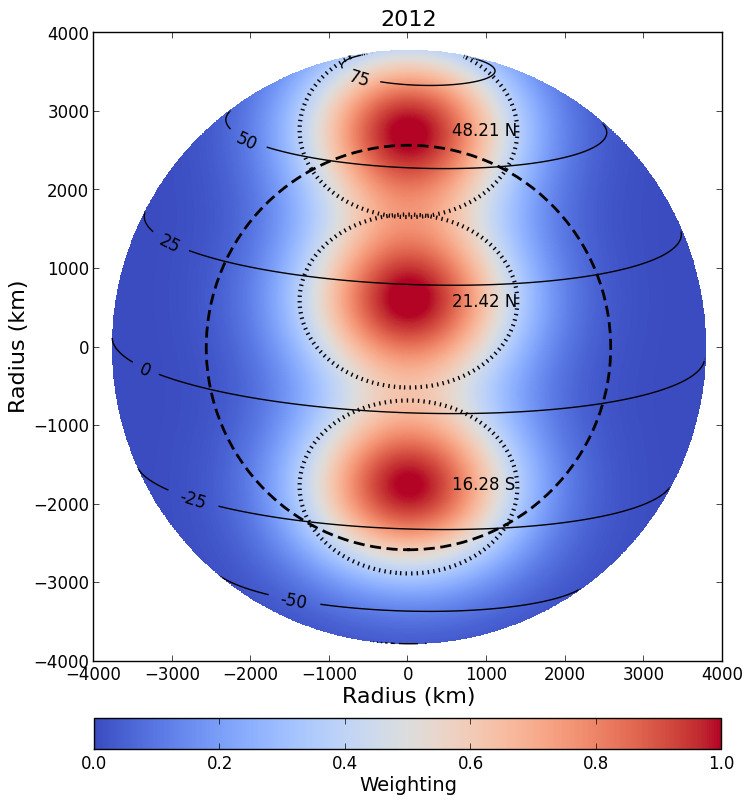
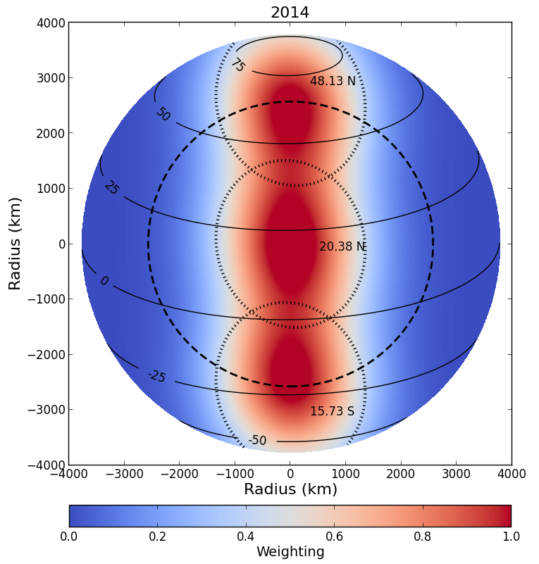
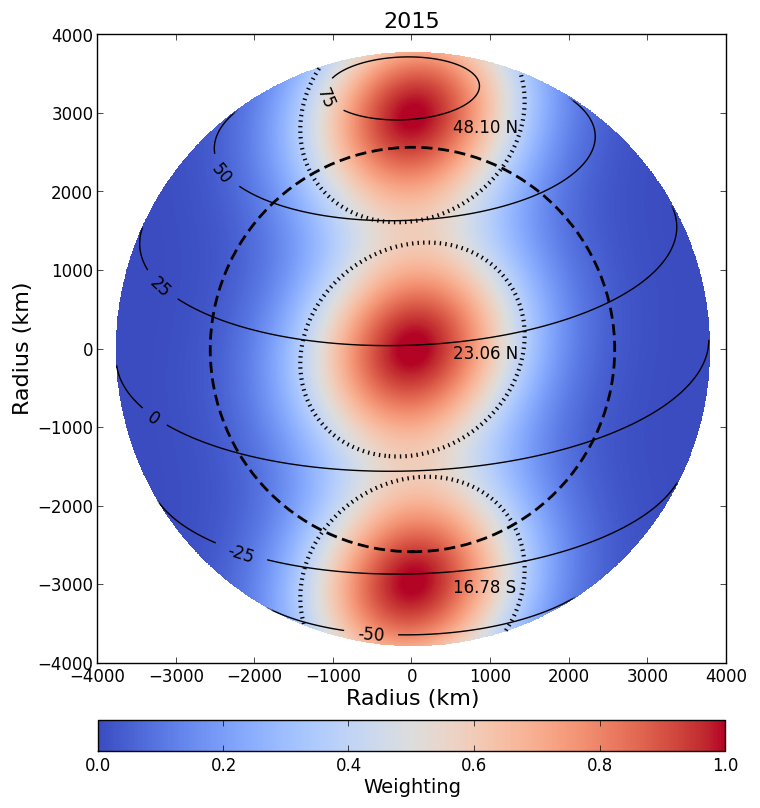
Figure 1: Representative spatial regions for ALMA 2012 (left panel), 2014 (center), and 2015 (right) images of Titan. Titan’s solid body radius is shown as a dashed circle. Solid lines trace the top-of-atmosphere (1200 km above the surface) latitudes. Color scale represents weighting given to emission angles for radiative transfer modeling. Beam-footprints are placed such that the mean latitude of each region (printed) does not change by more than $5^{\circ}$ from year to year, while also limiting the flux contribution from adjacent regions. Titan’s tilt is also accounted for, which changed by $\sim 12^{\circ}$ from 2012–2015. Weighting contributions are not coadded, as plotted here. The beam FWHM corresponding to each extracted spectrum is shown with a dotted ellipse.

Table 2: Cassini Data

Date	Titan	Latitude	Altitude	LS
	Flyby	Coveragea	Range (km)	(∘)
CIRS
06 Jun 2012	T84	80.0∘ S – 72.5∘ N	100–300	34.05
02 Feb 2014	T98	90.0∘ S – 87.5∘ N	100–300	53.16
07 Apr 2014	T100	90.0∘ S – 90.0∘ N	100–300	55.15
07 Jul 2015	T112	67.5∘ S – 72.5∘ N	100–300	69.17
Radio Occultation Science
26 Mar 2007	T27	69.0∘ S, 52.9∘ N	0–300	329.52
28 May 2007	T31	74.3∘ S, 74.1∘ N	0–300	331.78
03 Nov 2008	T46	32.4∘ S, –	0–300	350.32
22 Jun 2009	T57	79.8∘ N, –	0–300	358.29

Notes: ^aLatitude coverage for Cassini CIRS nadir measurements are continuous, with 2.5^∘ latitude bins; radio occultation science latitudes are given for ingress and egress observations (near the surface), respectively.

Table 3: Statistical Tests

Measurement	Radio Science		CIRS
	Da	$\alpha$b	D	$\alpha$
Disk-Averaged
2012	0.12	0.99	0.18	0.99
2013	0.16	0.88	0.18	0.99
2014	0.16	0.88	0.27	0.74
2015	0.16	0.88	0.18	0.99
Spatially Resolved
2012 (South)	0.08	0.99	0.12	0.99
2012 (Center)	0.24	0.41	0.09	1.00
2012 (North)	0.24	0.41	0.09	1.00
2014 (South)	0.20	0.65	0.27	0.74
2014 (Center)	0.12	0.99	0.18	0.99
2014 (North)	0.20	0.65	0.27	0.74
2015 (South)	0.16	0.88	0.18	0.99
2015 (Center)	0.20	0.65	0.18	0.99
2015 (North)	0.12	0.99	0.09	1.00

Notes: ^aKS test statistic. ^bSignificance level of KS test statistic.

References

- [1] R. K. Achterberg, B. J. Conrath, P. J. Gierasch, F. M. Flasar and C. A. Nixon “Titan’s middle-atmospheric temperatures and dynamics observed by the Cassini Composite Infrared Spectrometer” In Icarus 194, 2008, pp. 263–277
- [2] R. K. Achterberg, P. J. Gierasch, B. J. Conrath, F. M. Flasar and C. A. Nixon “Temporal variations of Titan’s middle-atmosphere temperatures from 2004 to 2009 observed by Cassini/CIRS” In Icarus 211, 2011, pp. 686–698
- [3] R. K. Achterberg, P. J. Gierasch, B. J. Conrath, F. M. Flasar, D. E. Jennings and C. A. Nixon “Post-equinox variations of Titan’s mid-stratospheric temperatures from Cassini/CIRS observations” In DPS Meeting 46, 2014
- [4] R. K. et al. Achterberg “[Dataset] CIRS Nadir Temperature Retrievals” In Mendeley Data, v1, 2017 DOI: 10.17632/f3b9zj96tm.1
- [5] A. Borysow “Modeling of collision-induced infrared absorption spectra of H2-H2 pairs in the fundamental band at temperatures from 20 to 300 K” In Icarus 92, 1991, pp. 273–279
- [6] A. Borysow and L. Frommhold “Collision-induced rototranslational absorption spectra of N2-N2 pairs for temperatures from 50 to 300 K” In ApJ 311, 1986a, pp. 1043–1057
- [7] A. Borysow and L. Frommhold “Theoretical collision-induced rototranslational absorption spectra for modeling Titan’s atmosphere: H2-N2 pairs” In ApJ 303, 1986b, pp. 495–510
- [8] A. Borysow and L. Frommhold “Theoretical collision-induced rototranslational absorption spectra for the outer planets: H2-CH4 pairs” In ApJ 304, 1986c, pp. 849–865
- [9] A. Borysow and L. Frommhold “Collision-induced rototranslational absorption spectra of CH4-CH4 pairs at temperatures from 50 to 300 K” In ApJ 318, 1987, pp. 940–943
- [10] A. Borysow and C. Tang “Far infrared CIA spectra of N2-CH4 pairs for modeling of Titan’s atmosphere” In Icarus 105, 1993, pp. 175–183
- [11] M. A. Cordiner et al. “ALMA measurements of the HNC and HC3N distributions in Titan’s atmosphere” In ApJ 795, 2014, pp. L30–L35
- [12] M. A. Cordiner et al. “Ethyl cyanide on Titan: spectroscopic detection and mapping using ALMA” In ApJ 800, 2015, pp. L14–L19
- [13] R. Courtin, B. M. Swinyard, R. Moreno, T. Fulton, E. Lellouch, M. Rengel and P. Hartogh “First results of Herschel-SPIRE observations of Titan” In AA 536, 2011, pp. L2
- [14] A. Coustenis et al. “Titan’s temporal evolution in stratospheric trace gases near the poles” In Icarus 270, 2016, pp. 409–420
- [15] C. Bergh et al. “Applications of a new set of methane line parameters to the modeling of Titan’s spectrum in the m window” In Planet. Space Sci. 61, 2012, pp. 85–98
- [16] R. Kok et al. “Oxygen compounds in Titan’s stratosphere as observed by Cassini CIRS” In Icarus 186, 2007, pp. 354–363
- [17] F. M. Flasar, R. E. Samuelson and B. J. Conrath “Titan’s atmosphere: temperature and dynamics” In Nature 292, 1981, pp. 293–298
- [18] F. M. Flasar et al. “Titan’s atmospheric temperatures, winds, and composition” In Science 308, 2005, pp. 975–978
- [19] F. M. Flasar, R. K. Achterberg and P. J. Schinder “Thermal structure of Titan’s troposphere and middle atmosphere” In Titan Cambridge, UK: Cambridge University Press, 2014, pp. 102
- [20] M. Fulchignoni et al. “In situ measurements of the physical characteristics of Titan’s environment” In Nature 438, 2005, pp. 785–791
- [21] C. A. Griffith, S. Rafkin, P. Rannou and C. P. McKay “Storms, clouds, and weather” In Titan Cambridge, UK: Cambridge University Press, 2014, pp. 190
- [22] M. Gurwell “Submillimeter observations of Titan: global measures of stratospheric temperature, CO, HCN, HC3N, and the isotopic ratios of 12C/13C and 14N/15N” In ApJ 616, 2004, pp. L7–L10
- [23] M. Gurwell and D. O. Muhleman “CO on Titan: more evidence for a well-mixed vertical profile” In Icarus 145, 2000, pp. 653–656
- [24] M. Gurwell, R. Moreno, A. Moullet and B. Butler “Titan’s stratosphere: isotopic ratios of CO and HCN” In EPSC-DPS Joint Meeting 2011, 2011
- [25] P. G. J. Irwin et al. “The NEMESIS planetary atmosphere radiative transfer and retrieval tool” In J. Quant. Spec. Radiat. Transf. 109, 2008, pp. 1136–1150
- [26] V. A. Krasnopolsky “Chemical composition of Titan’s atmosphere and ionosphere: observations and the photochemical model” In Icarus 236, 2014, pp. 83–91
- [27] S. Lebonnois, J. Burgalat, P. Rannou and B. Charnay “Titan global climate model: a new 3-dimensional version of the IPSL Titan GCM” In Icarus 218, 2012, pp. 707–722
- [28] E. Lellouch et al. “Titan’s m window: observations with the Very Large Telescope” In Icarus 162, 2003, pp. 125–142
- [29] J. C. Loison et al. “The neutral photochemistry of nitriles, amines and imines in the atmosphere of Titan” In Icarus 247, 2015, pp. 218–247
- [30] E. M. Molter et al. “ALMA observations of HCN and its isotopologues on Titan” In AJ 152, 2016, pp. 1–7
- [31] H. S. P. Müller, S. Thorwirth, D. A. Roth and G. Winnewisser “The Cologne Database for Molecular Spectroscopy, CDMS” In AA 370, 2001, pp. L49–L52
- [32] C. E. Newman, C. Lee, Y. Lian, M. I. Richardson and A. D. Toigo “Stratospheric superrotation in the TitanWRF model” In Icarus 213, 2011, pp. 636–654
- [33] H. B. Niemann et al. “The abundances of constituents of Titan’s atmosphere from the GCMS instrument on the Huygens probe” In Nature 438, 2005, pp. 779–784
- [34] H. B. Niemann et al. “Composition of Titan’s lower atmosphere and simple surface volatiles as measured by the Cassini-Huygens probe gas chromatograph mass spectrometer experiment” In JGR 115, 2010 DOI: 10.1029/2010JE003659
- [35] Maureen Y. Palmer et al. “ALMA detection and astrobiological potential of vinyl cyanide on Titan” In Sci. Adv. 3.7, 2017 DOI: 10.1126/sciadv.1700022
- [36] M. Rengel, H. Sagawa and P. Hartogh “New sub-millimeter heterodyne observations of CO and HCN in Titan’s atmosphere with the APEX Swedish Heterodyne Facility Instrument” In Adv. in Geosci. Vol. 25: Planetary Science, 2011, pp. 173–185
- [37] M. Rengel et al. “Herschel/PACS spectroscopy of trace gases of the stratosphere of Titan” In Astronomy Astrophysics 561, 2014, pp. 1–6
- [38] L. S. Rothman et al. “The HITRAN2012 molecular spectroscopic database” In J. Quant. Spec. Radiat. Transf. 130, 2013, pp. 4–50
- [39] P. J. Schinder et al. “The structure of Titan’s atmosphere from Cassini radio occultations” In Icarus 215, 2011, pp. 460–474
- [40] P. J. Schinder et al. “The structure of Titan’s atmosphere from Cassini radio occultations: occultations from the Prime and Equinox missions” In Icarus 221, 2012, pp. 1020–1031
- [41] J. Serigano, C. A. Nixon, M. A. Cordiner, P. G. J. Irwin, N. A. Teanby, S. B. Charnley and J. E. Lindberg “Isotopic ratios of carbon and oxygen in Titan’s CO using ALMA” In ApJ 821, 2016, pp. L8–L13
- [42] N. A. Teanby, P. G. J. Irwin, R. Kok and C. A. Nixon “Seasonal changes in Titan’s polar trace gas abundance observed by Cassini” In ApJ 724, 2010, pp. L84–L89
- [43] N. A. Teanby, P. G. J. Irwin, R. Kok and C. A. Nixon “Mapping Titan’s HCN in the far infra-red: implications for photochemistry” In Faraday Discuss. 147, 2010, pp. 51–64
- [44] N. A. Teanby et al. “Active upper-atmosphere chemistry and dynamics from polar circulation reversal on Titan” In Nature 491, 2012, pp. 732–735
- [45] N. A. Teanby et al. “Constraints on Titan’s middle atmosphere ammonia abundance from Herschel/SPIRE sub-millimetre spectra” In Planet. Space Sci. 75, 2013, pp. 136–147
- [46] A. E. et al. Thelen “[Dataset] ALMA Titan Emission Angles” In Mendeley Data, v1, 2017 DOI: 10.17632/m5pscpthph.1
- [47] A. E. et al. Thelen “[Dataset] ALMA Titan Temperature Retrievals” In Mendeley Data, v1, 2017 DOI: 10.17632/xk3nkvz28b.1
- [48] S. Vinatier et al. “Vertical abundance profiles of hydrocarbons in Titan’s atmosphere at 15 S and 80 N retrieved from Cassini/CIRS spectra” In Icarus 188, 2007, pp. 120–138
- [49] S. Vinatier et al. “Seasonal variations in Titan’s middle atmosphere during the northern spring derived from Cassini/CIRS observations” In Icarus 250, 2015, pp. 95–115
- [50] Y. L. Yung, M. Allen and J. P. Pinto “Photochemistry of the atmosphere of Titan: comparison between model and observations” In ApJ SS 55, 1984, pp. 465–506