Heegaard Floer invariants of contact structures on links of surface singularities

Abstract.

Let a contact 3-manifold $(Y,\xi_{0})$ be the link of a normal surface singularity equipped with its canonical contact structure $\xi_{0}$. We prove a special property of such contact 3-manifolds of “algebraic” origin: the Heegaard Floer invariant $c^{+}(\xi_{0})\in HF^{+}(-Y)$ cannot lie in the image of the $U$-action on $HF^{+}(-Y)$. It follows that Karakurt’s “height of $U$-tower” invariants are always 0 for canonical contact structures on singularity links, which contrasts the fact that the height of $U$-tower can be arbitrary for general fillable contact structures. Our proof uses the interplay between the Heegaard Floer homology and Némethi’s lattice cohomology.

1. Introduction and background

Consider a complex surface $\Sigma\subset\mathbb{C}^{N}$ with an isolated critical point at the origin. For a sufficiently small $\varepsilon>0$, the intersection $Y=\Sigma\cap S^{2N-1}_{\varepsilon}$ with the sphere $S^{2N-1}_{\varepsilon}=\{|z_{1}|^{2}+|z_{2}|^{2}+\dots+|z_{N}|^{2}=\varepsilon\}$ is a smooth 3-manifold called the link of the singularity. The complex structure on $\Sigma$ induces the canonical contact structure $\xi_{0}$ on $Y$ given by the distribution of complex tangencies; in this setting, $(Y,\xi_{0})$ is also called Milnor fillable. The contact manifold $(Y,\xi_{0})$ is independent of the choice of $\varepsilon$, up to contactomorphism. Moreover, it is shown in [CNP] that the Milnor fillable contact structure on $Y$ is unique (note that in general, a link of singularity may support a number of tight or Stein fillable contact structures). The Milnor fillable structure can be thought of as the contact structure closely related to the algebraic origin of the manifold $Y$ as link of singularity (and potentially carry information about the singularity). We would like to address

Question 1.1.

Are there any special features that distinguish the canonical contact structure from other contact structures on the link of singularity?

It is known, for example, that $\xi_{0}$ is always Stein fillable [BO] and universally tight [LO]. In this paper, we work with Ozsváth-Szabó’s Heegaard Floer homology [OS1] and Némethi’s lattice cohomology [Ne2, Ne3] to establish special properties of the Heegaard Floer contact invariant $c^{+}$ (introduced in [OS3]) of canonical contact structures. Recall that for a $3$-manifold $Y$, the Heegaard Floer homology $HF^{+}(Y)$ is an $\mathbb{F}[U]$-module (coefficients are assumed to be $\mathbb{F}=\mathbb{Z}/2$, see Remark 5.7 for $\mathbb{Z}$ coefficients). We review the context and background after stating our main result in terms of the $U$-action.

Theorem 1.2.

Let $(Y,\xi_{0})$ be a rational homology sphere link of a normal surface singularity with its canonical contact structure, and $c^{+}(\xi_{0})\in HF^{+}(-Y)$ its contact invariant. Assume that the singularity is not rational. Then $c^{+}(\xi)\notin\operatorname{Im}U$.

A singular point $p$ is normal when bounded holomorphic functions defined in its punctured neighborhood can be extended over $p$. More importantly to us, normality together with the homological assumption on $Y$ is equivalent to saying that $Y$ is the boundary of a negative-definite 4-manifold which is a plumbing of spheres such that the plumbing graph is a tree (see section 2).

Given a 3-manifold $Y$, recall that its Heegaard Floer homology, developed in [OS1] and sequels, is an $\mathbb{F}[U]$-module $HF^{+}(Y)$ that decomposes as a direct sum of components corresponding to $Spin^{c}$ structures on $Y$. When $Y$ is a rational homology sphere, $HF^{+}(Y,\mathfrak{s})=\mathcal{T}\oplus\mathrm{Torsion}$, where $\mathcal{T}$ is isomorphic to $\mathbb{F}[U,U^{-1}]/U\mathbb{F}[U]$ (with the appropriate grading) and $\mathrm{Torsion}$ is annihilated by $U^{d}$ for some large $d$. A rational homology sphere $Y$ is called an $L$-space when its Heegaard Floer homology is the simplest possible, i.e. $HF^{+}(Y,\mathfrak{s})=\mathcal{T}$ for every $\mathfrak{s}\in Spin^{c}(Y)$. In the case where $Y$ is the link of a normal surface singularity, it is known that $Y$ is an $L$-space if and only if the singularity is rational, [OS2, Ne4]. (We will not discuss algebro-geometric definition of rational singularities here; in fact the reader can take the $L$-space criterion above as a definition.)

Given a contact 3-manifold $(Y,\xi)$, its invariant $c^{+}(\xi)$ is defined as a distingushed element of the Heegaard Floer group $HF^{+}(-Y)$, [OS3]. More precisely, $c^{+}(\xi)\in HF^{+}(-Y,\mathfrak{t}_{\xi})$, where $\mathfrak{t}_{\xi}$ is the $Spin^{c}$ structure induced by $\xi$. For Stein fillable contact structures, the invariant is non-zero, in particular, $c^{+}(\xi_{0})\neq 0$ for the canonical contact structure $\xi_{0}$ on a link of any surface singularity. For an arbitrary contact 3-manifold $(Y,\xi)$, the contact invariant is annihilated by the $U$-action, i.e. $c^{+}(\xi)\in\operatorname{Ker}U$.

The $\mathbb{F}[U]$-module structure was used by Karakurt in [Ka] to define a related numerical invariant of contact structures. More precisely, Karakurt considers the height of $U$-tower over $c^{+}(\xi)$ to define

$$ht(\xi)=\max\{n:c^{+}(\xi)\in U^{n}\cdot HF^{+}(-Y)\}.$$

We have taken the liberty of changing the sign in Karakurt’s original definition; in [Ka], the invariant is defined as $\sigma(\xi)=-ht(\xi)$. Karakurt computes $ht$ for a number of contact structures obtained by Legendrian surgery, and shows that $ht$ can take arbitrary integer values from $0$ to $+\infty$. In [KO], Karakurt and Öztürk show that the height of tower is 0 for canonical contact structures on links of “almost rational” (AR) singularities, using the fact that Heegaard Floer homology is isomorphic to Némethi’s lattice cohomology [Ne2, Ne3] for 3-manifolds of this type. For rational singularities, it is easy to see that $ht=+\infty$ for every contact structure on the link: this follows from the fact that the link $Y$ of a rational singularity is an $L$-space, i.e. $HF^{+}(-Y,\mathfrak{s})=\mathcal{T}$ for every $Spin^{c}$ structure $s$ on $Y$, [OS2, Ne2]. Karakurt-Öztürk ask whether height of tower can take arbitrary integer values for canonical contact structures on links of general normal surface singularities [KO, Question 6.2]. It follows immediately from Theorem 1.2 that the answer is manifestly no:

Corollary 1.3.

Consider a normal surface singularity which is not rational and its link is a rational homology sphere. Let $\xi_{0}$ be the canonical contact structure on the link. Then $ht(\xi_{0})=0$.

When starting this work, our initial goal was to use the height of tower invariants (together with their monotonicity under Stein cobordisms [Ka]) to obstruct certain deformations of surface singularities. The above corollary means, however, that the $ht$ invariant contains very little information about the given singularity! (One could use $ht$ to show that rational singularities cannot be deformed into non-rational, but this is a well-known fact and a special case of the semicontinuity of the geometric genus, see [Elk]. The algebro-geometric proof of this fact is non-trivial, so the Heegaard Floer argument may still be of interest.)

Similarly to [KO], our proof also uses the interplay between Heegaard Floer homology and lattice cohomology of [Ne2, Ne3]. Lattice cohomology is defined in a combinatorial way, using the intersection lattice of the plumbing graph (the dual resolution graph of the singularity). Under certain rather restrictive conditions (for example, for links of AR singularities), the Heegaard Floer homology and lattice cohomology are known to be isomorphic [OS2, Ne3]. For arbitrary 3-manifolds, a spectral sequence from lattice homology to Heegaard Floer homology was found in [OSS]; this spectral sequence collapses in certain special cases, but in general, isomorphism between Heegaard Floer and lattice (co)homologies has not been established. The isomorphism between the Heegaard Floer and lattice theories in the case of AR singularities is the key tool in Karakurt’s and Karakurt-Öztürk’s proofs in [Ka, KO]. Our approach is different in that we only use an $\mathbb{F}[U]$-equivariant map from the Heegaard Floer homology to the lattice cohomology and do not require an isomorphism, thus our argument works in general. The homomorphism we use comes from [OS2] and maps $HF^{+}(-Y)$ to the $0$-dimensional part $\mathbb{H}_{0}^{+}(\Gamma)$ of lattice cohomology. (The latter is much simpler that the full lattice cohomology $\mathbb{H}^{\ast}(\Gamma)$; note that for AR-singularities, lattice cohomology vanishes in dimensions $n>0$, [LN].) Another difference between our work and [KO] is that we use general properties of graded roots without resorting to Laufer sequences specific to the AR case. Finally, although this is not stated explicitly, the proofs in [KO] only work if the minimal resolution of the singularity has exceptional divisor with normal crossings (see discussion in Section 2 and Section 5). This condition often fails, even for AR singularities; we give a proof for the general case.

It is intriguing that the proof of Theorem 1.2 works with lattice cohomology to establish a statement about Heegaard Floer invariants, even in the absence of isomorphism between the two theories. It would be very interesting to find further similar applications of lattice cohomology.

The paper is organized as follows. In Sections 2 and 3, we collect some background facts on resolutions and describe different constructions of lattice cohomology. In Section 4, we prove Theorem 1.2 under the additional assumption that there is a good resolution that carries a Stein structure; in the general case we indicate how the proof of Theorem 1.2 follows from some technical lemmas that are relegated to Section 5. Section 5 examines lattice homology in presence of blowups and completes the proof of Theorem 1.2.

Acknowledgements:

We would like to thank the referee for pointing out a mistake in the first version of the article (Section 5 was added to correct that mistake). The second author thanks Marco Golla and Oleg Viro for some useful discussions and comments.

2. Resolutions and plumbing graphs

Consider a resolution $\pi:\tilde{\Sigma}\to\Sigma$ of a normal surface singularity $(\Sigma,0)$. The inverse image in $\tilde{\Sigma}$ of a small neighborhood of $0$ in $\Sigma$ is a 4-manifold $X$ with $\partial X=Y$, where $Y$ is the link of the singularity. If the resolution is minimal (i.e. $X$ has no smooth rational curves of self-intersection $-1$), by [BO] the manifold $X_{min}$ carries a Stein structure $J$ so that $(X,J)$ is a Stein filling for the canonical contact structure $\xi_{0}$ on $Y$.

Our main tool in this paper is lattice homology, an invariant constructed from a good resolution of $(\Sigma,0)$. A resolution is good if the irreducible components of the exceptional divisor $\pi^{-1}(0)$ are smooth complex curves that intersect transversely at double points only. (In other words, $\pi^{-1}(0)$ is required to be a normal crossing divisor.) The dual resolution graph $\Gamma$ is the graph whose vertices correspond to irreducible components of the exceptional divisor and the edges record intersections of these components. Each vertex is decorated with an integer weight equal to the self-intersection of the corresponding curve. The resolution yields a 4-manifold $X(\Gamma)$ such that $\partial X(\Gamma)=Y$, where $Y$ is the link of singularity. For normal singularities, $X(\Gamma)$ is negative-definite, and $Y$ is a rational homology sphere if and only if $\Gamma$ is a tree and each vertex corresponds to a 2-sphere. (See for example [Ne3, §2.1-2.2] for details.) The manifold $X(\Gamma)$ can be obtained by plumbing disk bundles over 2-spheres (with Euler numbers given by weights of vertices) as dictated by the graph $\Gamma$, so $\Gamma$ is often called a plumbing graph. If the resolution of a normal singularity $(\Sigma,0)$ is not good, it can still be encoded by a graph $\Gamma$, but one needs to record the singularities of the components of the exceptional divisor and specify multiple intersections.

It is important to note that the minimal resolution of $(\Sigma,0)$ does not have to be good, but one can always obtain a good resolution from a minimal resolution by some blowups. (This is a standard fact, see for example [Ha, Theorem V.3.9] for a closely related result. See also [Ne1, §1] for discussion and examples; bad minimal resolutions can appear even in very simple situations.) Accordingly, a good resolution does not have to be minimal, so $X(\Gamma)$ is not Stein in general. However, $X(\Gamma)$ always carries a symplectic form $\omega_{0}$ such that $(X(\Gamma),\omega_{0})$ is a strong symplectic filling for $(Y,\xi_{0})$. Indeed, $\tilde{\Sigma}$ is Kähler since it lives in a blowup of $\mathbb{C}^{N}$, in particular, $\tilde{\Sigma}$ has a symplectic form $\omega_{0}$ compatible with the complex structure. For a good resolution, the irreducible components of the exceptional divisor $\pi^{-1}(0)$ are smooth complex curves, thus they are symplectic surfaces in $X(\Gamma)\subset\tilde{\Sigma}$ with respect to $\omega_{0}$. The contact manifold $(Y,\xi_{0})$ is the convex boundary of the plumbing $X(\Gamma)$ of these symplectic surfaces.

We work with bad minimal resolutions and their good blowups in Section 5. We need a minimal resolution to use the Stein structure, but if $\pi^{-1}(0)$ is not a normal crossing divisor, $X_{min}$ cannot be used to define the lattice homology of the link. We will need to perform some additional blowups on $X_{min}$ to obtain a complex surface $X$ which is a good resolution with plumbing graph $\Gamma$, and examine special features of the lattice homology construction in presence of $(-1)$ vertices of $\Gamma$.

3. Lattice Cohomology

In this section, we discuss the necessary background on lattice cohomology, [OS2, Ne2, Ne3]. Lattice cohomology $\mathbb{H}^{\ast}(\Gamma)$ was defined by Némethi in [Ne3] as a combinatorial theory conjecturally parallel to Heegaard Floer homology. Starting with a plumbing graph $\Gamma$ that defines a 4-manifold with boundary $X(\Gamma)$, Némethi’s construction uses cellular cohomology of certain $CW$-complexes associated to the lattice $L=H_{2}(X(\Gamma),\mathbb{Z})$ equipped with a weight function. We do not give the general definition of $\mathbb{H}^{\ast}(\Gamma)$ here as we will only work with its $0$-dimensional part $\mathbb{H}_{0}^{+}(\Gamma)$. (The reader will get a glimpse of the CW-complexes in the graded roots discussion below.) However, we will use several equivalent definitions of the 0-dimensional cohomology, those from [Ne3] and its precursors [OS2, Ne2]. We also use specific isomorphisms between these constructions, so we review this material in some detail. (Everything we need is contained in [Ne2] but some of the statements are implicit and somewhat difficult to extract from [Ne2].)

As before, let $Y$ be a rational homology sphere which is a link of normal surface singularity. Let $\Gamma$ be a negative-definite connected plumbing graph as above, defining a $4$-manifold $X=X(\Gamma)$ with boundary $\partial X=Y=Y(\Gamma)$.

Consider the lattice $L=H_{2}(X,\mathbb{Z})$; the intersection form on $L$ can be read off the graph $\Gamma$. Indeed, the vertices of $\Gamma$ give a basis for $L$; $v$ will usually denote both a vertex and its corresponding homology class. Then, the self-intersection $v\cdot v$ equals the weight decoration of the vertex $v$, and for two different vertices $v,w$ we have $v\cdot w=1$ if $v,w$ are connected by an edge in $\Gamma$, and $0$ otherwise.

Set $L^{\prime}=H^{2}(X,\mathbb{Z})$ and $H=H_{1}(Y,\mathbb{Z})$. Since $X$ has no $1$-handles, from Poincaré duality, the universal coefficient theorem and the homology exact sequence of the pair $(X,Y)$ we have

$$L^{\prime}=H^{2}(X,\mathbb{Z})\simeq H_{2}(X,Y,\mathbb{Z})\simeq\operatorname{Hom}(H_{2}(X,\mathbb{Z}),\mathbb{Z}),$$

and our assumption that $Y$ is a rational homology sphere gives a short exact sequence $0\rightarrow L\rightarrow L^{\prime}\rightarrow H\rightarrow 0$. We will use the map $\operatorname{PD}:L\rightarrow L^{\prime}$ defined by composing the Poincaré duality $H_{2}(X,\mathbb{Z})\rightarrow H^{2}(X,Y,\mathbb{Z})$ with the cohomological inclusion $H^{2}(X,Y,\mathbb{Z})\rightarrow H^{2}(X)$.

Let $\operatorname{Char}(\Gamma)\subset H^{2}(X,\mathbb{Z})$ be the set of characteristic vectors, that is,

$$\operatorname{Char}=\operatorname{Char}(\Gamma)=\{K\in L^{\prime}:\langle K,x\rangle\equiv x\cdot x\ (\textrm{mod\ }2)\ \ \forall x\in L\},$$

where $\langle K,x\rangle$ is the evaluation of $K\in L^{\prime}=H^{2}(X,\mathbb{Z})\simeq\operatorname{Hom}(H_{2}(X,\mathbb{Z}),\mathbb{Z})$ on $x\in H_{2}(X,\mathbb{Z})$ and $x\cdot x$ is the self-intersection of $x$ by the intersection form on $L=H_{2}(X,\mathbb{Z})$.

We have $\operatorname{Char}=K+2L^{\prime}$ for any fixed $K\in\operatorname{Char}$. The natural action $K\mapsto K+2\operatorname{PD}(x)$ (for any $x\in L$) of $L$ on $\operatorname{Char}$ has orbits of form $K+2\operatorname{PD}(L)$. We will denote an orbit of this form by $[K]\subset\operatorname{Char}$.

Since $X(\Gamma)$ is simply connected, $\operatorname{Char}(\Gamma)$ is isomorphic to the set of $Spin^{c}$ structures on $X$, and the identification is given by the first Chern class of the determinant line bundle associated with a given $Spin^{c}$ structure (see e.g. [GS, Proposition 2.4.16]). If $\mathfrak{s}$ is any fixed $Spin^{c}$ structure on $X$ and $\mathfrak{t}=\mathfrak{s}|_{Y}$ is its restriction to $Y$, the $Spin^{c}$ structures on $X$ which restrict to $\mathfrak{t}$ are exactly those whose first Chern classes form an orbit of form $[K]=K+2\operatorname{PD}(L)$, where $K=c_{1}(\mathfrak{s})\in\operatorname{Char}(\Gamma)$. Thus, $Spin^{c}$ structures on $Y$ can be identified with orbits of the $L$-action on $\operatorname{Char}(X)$, and we will sometimes use the notation $\mathfrak{t}=[K]\in Spin^{c}(Y)$.

For any $K\in\operatorname{Char}$, we will also consider the (in general, rational) number $K^{2}$ defined by using the intersection pairing on $H^{2}(X;\mathbb{Q})\simeq H_{2}(X,Y;\mathbb{Q})\simeq H_{2}(X,\mathbb{Q})$ (the latter isomorphism holds because $Y$ is a rational homology sphere). Rational coefficients are needed since $H^{2}(X;\mathbb{Z})\simeq H_{2}(X,Y;\mathbb{Z})$ doesn’t have a well-defined intersection pairing.

All the lattice cohomologies discussed below are taken with coefficients in $\mathbb{F}=\mathbb{Z}/2$ and have the structure of $\mathbb{F}[U]$-modules (these modules are graded but we omit the gradings since they will not be important to us). See Remark 5.7 for coefficients in $\mathbb{Z}$.

Let $\mathcal{T}_{0}^{+}$ denote the module $\mathbb{F}[U,U^{-1}]/U\cdot\mathbb{F}[U]$. We will use the notation $1=U^{0}\in\mathcal{T}_{0}^{+}$ for the corresponding generator.

3.1. Lattice cohomology via functions on Char.

This is a review of the construction due to Ozsváth and Szabó, [OS2, §1].

Define a weight function $w$ on $\operatorname{Char}$ by setting $w(K)=-(K^{2}+|\Gamma|)/8$, where $|\Gamma|$ stands for the number of vertices in the plumbing graph, i.e. the number of basis elements of $H_{2}(X,\mathbb{Z})$ provided by the exceptional divisors.

Definition 3.1.

The 0-dimensional lattice cohomology $\mathbb{H}_{0}^{+}(\Gamma)\subset\operatorname{Hom}(\operatorname{Char}(\Gamma),\mathcal{T}_{0}^{+})$ is the set of functions satisfying the following adjunction relations for characteristic vectors $K\in\operatorname{Char}(\Gamma)$ and vertices $v$ of $\Gamma$. If $n$ is an integer such that $2n=\langle K,v\rangle+v\cdot v$ (or, equivalently, $w(K)-w(K+2\operatorname{PD}(v))=n$), we require for every $\phi\in\mathbb{H}_{0}^{+}(\Gamma)\subset\operatorname{Hom}(\operatorname{Char}(\Gamma),\mathcal{T}_{0}^{+})$ that

$$U^{n}\cdot\phi(K+2\operatorname{PD}[v]) =\phi(K) \text{ if }n\geq 0,$$ (1)

$$\phi(K+2\operatorname{PD}[v]) =U^{-n}\cdot\phi(K) \text{ if }n\leq 0.$$

We introduce $U$-action on $\mathbb{H}^{+}_{0}(\Gamma)$ by setting $(U\phi)(K)=U(\phi(K))$ for every characteristic vector $K\in\operatorname{Char}(\Gamma)$, thus $\mathbb{H}^{+}_{0}(\Gamma)$ becomes an $\mathbb{F}[U]$-module.

As the compatibility condition (1) above involves relations between elements of $\operatorname{Char}(\Gamma)$ that differ by an element in $2\operatorname{PD}(L)$, the $\mathbb{F}[U]$-module $\mathbb{H}^{+}_{0}(\Gamma)$ decomposes as a direct sum according to the $Spin^{c}$ structures on $Y$:

$$\mathbb{H}^{+}_{0}(\Gamma)=\bigoplus_{\mathfrak{t}\in Spin^{c}(Y)}\mathbb{H}^{+}_{0}(\Gamma,\mathfrak{t}).$$

We will use the notation $\mathbb{H}^{+}_{0}(\Gamma,[K])$ to denote the direct summand of the above decomposition which corresponds to the $Spin^{c}$ structure $\mathfrak{t}$. Here, $[K]$ is the $L$-orbit formed by the first Chern classes of $Spin^{s}$ structures on $X$ restricting to $\mathfrak{t}$ on $Y$. One can think of elements of $\mathbb{H}^{+}_{0}(\Gamma,[K])$ as functions in $\operatorname{Hom}([K],\mathcal{T}_{0}^{+})$ satisfying the compatibility conditions (1).

3.2. Lattice cohomology via functions on homology lattice.

We now describe a slightly different construction by Némethi, introduced in [Ne2, Proposition 4.7].

Given any characteristic element $K\in\operatorname{Char}(\Gamma)$, define the weight function $\chi_{K}$ on $L$ such that for any $x\in L$ we set

$$\chi_{K}(x)=-\frac{1}{2}(\langle K,x\rangle+x\cdot x).$$ (2)

Definition 3.2.

For a fixed characteristic vector $K\in\operatorname{Char}(\Gamma)$, the lattice cohomology $\mathbb{H}\mathbb{L}_{0}^{+}(\Gamma,K)\subset\operatorname{Hom}(L,\mathcal{T}_{0}^{+})$ is the set of functions $\varphi:L\to\mathcal{T}^{+}_{0}$ satisfying the following relations for elements $x\in L$ and vertices $v$ of $\Gamma$. If $n$ is an integer such that $2n=\langle K,v\rangle+v\cdot v+2x\cdot v$, or, equivalently, if $\chi_{K}(x)-\chi_{K}(x+v)=n$ we require that

$$U^{n}\cdot\varphi(x+v) =\varphi(x) \text{ if }n\geq 0,$$ (3)

$$\varphi(x+v) =U^{-n}\cdot\varphi(x) \text{ if }n\leq 0.$$

This is also naturally an $\mathbb{F}[U]$ module by setting $(U\varphi)(x)=U(\varphi(x))$.

Lemma 3.3.

[Ne2, Proposition 4.7]

$$\mathbb{H}\mathbb{L}_{0}^{+}(\Gamma,K)\cong\mathbb{H}_{0}^{+}(\Gamma,[K]).$$

Proof.

The isomorphism is constructed as follows. Let $\iota_{K}:L\rightarrow[K]=K+2\operatorname{PD}(L)\subset\operatorname{Char}$ be the mapping defined by $\iota_{K}(x)=K+2\operatorname{PD}(x)$. Let $\iota_{K}^{*}:\mathbb{H}^{+}_{0}(\Gamma,[K])\rightarrow\mathbb{H}\mathbb{L}^{+}_{0}(\Gamma,K)$ be the induced dual map, that is, $\operatorname{Hom}(L,\mathcal{T}_{0}^{+})\ni\varphi=\iota_{K}^{*}(\phi)$ for $\phi\in\operatorname{Hom}([K],\mathcal{T}_{0}^{+})$ if $\varphi=\phi\circ\iota_{K}$. This map is well-defined as the two compatibility conditions (1) and (3) correspond to each other: setting $K^{\prime}=K+2\operatorname{PD}(x)$, we see that for a basis element $v$ of $L$ corresponding to a vertex of the plumbing graph,

$$\langle K^{\prime},v\rangle+v\cdot v=\langle K,v\rangle+v\cdot v+2x\cdot v.$$

In the language of the weight functions, this is exactly the fact $w(\iota_{K}(x+v))-w(\iota_{K}(x))=\chi_{K}(x+v)-\chi_{K}(x)$. ∎

3.3. Lattice cohomology via graded roots

Here we review Némethi’s main construction from [Ne2, § 4].

Fix $K\in\operatorname{Char}(\Gamma)$ and again consider the weight function $\chi_{K}:L\to\mathbb{Z}$ defined by equation (2) above. We consider sublevel sets of the function $\chi_{K}$ in the lattice $L$. For each $n\in\mathbb{Z}$, let $\bar{L}_{K,\leq n}$ be a finite 1-dimensional cell complex whose $0$-skeleton is the set

$$L_{K,\leq n}=\{x\in L:\chi_{K}(x)\leq n\},$$

and the $1$-cells are constructed as follows. If $x\in L$ and $v$ is the basis element of $L=H_{2}(X,\mathbb{Z})$ corresponding to a vertex of $\Gamma$, then we connect $x$ and $x+v$ by a unique 1-cell in $\bar{L}_{K,\leq n}$ whenever $x$ and $x+v$ are both in $L_{K,\leq n}$. Clearly, such cell complexes can be built as subsets of $L\otimes\mathbb{R}$, taking the 1-cells to be straight line segments connecting their endpoints. Then we have $\bar{L}_{K,\leq n}\subset\bar{L}_{K,\leq m}$ for $n<m$.

Consider the set $\pi_{0}(\bar{L}_{K,\leq n})$ of the connected components of $\bar{L}_{K,\leq n}$, and let $C_{w}$ denote the component corresponding to $w\in\pi_{0}(\bar{L}_{K,\leq n})$. If $m>n$, each $C_{w}$ is contained in a component $C_{w^{\prime}}$ for some $w^{\prime}\in\pi_{0}(\bar{L}_{K,\leq m})$, and $C_{w^{\prime}}$ may contain several distinct components of $\bar{L}_{K,\leq n}$. These inclusion relations are codified by the graded root $(R_{K},\chi_{K})$, which is a graph with an integer-valued grading function. The grading on the graph is closely related to the $U$-action on cohomology.

The vertices $\mathcal{V}(R_{K})$ of $(R_{K},\chi_{K})$ are given by the set $\cup_{n\in\mathbb{Z}}\pi_{0}(\bar{L}_{K,\leq n})$. The grading, $\mathcal{V}(R_{K})\to\mathbb{Z}$, still denoted by $\chi_{K}$, is defined by $\chi_{K}|_{\pi_{0}(\bar{L}_{K,\leq n})}=n$. Finally, all edges are obtained by connecting vertices of the form $w_{n}\in\pi_{0}(\bar{L}_{K,\leq n})$ and $w_{n+1}\in\pi_{0}(\bar{L}_{K,\leq n+1})$ such that $C_{w_{n}}\subset C_{w_{n+1}}$, where the inclusion is understood in the sense described above.

Remark 3.4.

As we mentioned, the elements of $\operatorname{Char}(\Gamma)$ fall into equivalence classes of form $[K]$ corresponding to $Spin^{c}$ structures on $Y$. It turns out that the graded roots corresponding to two characteristic elements $K,K^{\prime}$ belonging to the same orbit (that is, $K-K^{\prime}\in 2\operatorname{PD}(L)$) are the same up to a grading shift, so one can associate a well-defined graded root $(R_{\mathfrak{t}},\chi_{\mathfrak{t}})$ to a $Spin_{c}$ structure $\mathfrak{t}\in Spin^{c}(Y)$ if one fixes the grading so that $\min\chi_{\mathfrak{t}}|_{R_{\mathfrak{t}}}=0$, see [Ne2, Section 4] for details. As we do not work with absolute gradings on cohomology modules, we will not make the grading shift and will simply use the grading given by $\chi_{K}$.

Definition 3.5.

Fix a characteristic element $K\in\operatorname{Char}$, let $\chi_{K}$ be a weight function as in (2), and consider the graded root $(R_{K},\chi_{K})$ as above with the vertex set $\mathcal{V}=\mathcal{V}(R_{K})$. The associated $\mathbb{F}[U]$ module $\mathbb{H}(R,\chi)$ is defined as the set of functions $\psi:\mathcal{V}\to\mathcal{T}_{0}^{+}$ satisfying the condition

$$U\cdot\psi(v)=\psi(w)\text{ if }v,w\text{ are connected by an edge of }R\text{ and }\chi(v)<\chi(w).$$ (4)

Note that by the construction of the graded root, for $v,w$ as above we have in fact $\chi(v)+1=\chi(w)$. As before, there is obvious $U$-action on $\mathbb{H}(R,\chi)$, so that $(U\psi)(v)=U(\psi(v))$. See [Ne2, Definition 3.5] and discussion therein for details.

Lemma 3.6.

[Ne2, Proposition 4.7]

$$\mathbb{H}\mathbb{L}_{0}^{+}(\Gamma,K)\cong\mathbb{H}(R_{K},\chi_{K}).$$

Proof.

The isomorphism of [Ne2, Proposition 4.7] is constructed as follows. For an element $x\in L$ with $\chi_{K}(x)=n$, the map $\theta:L\rightarrow\mathcal{V}(R_{K})$ associates to $x$ the component of $\pi_{0}(\bar{L}_{K,\leq n})$ containing $x$.

This induces a map $\theta^{*}:\operatorname{Hom}(\mathcal{V}(R_{K}),\mathcal{T}_{0}^{+})\rightarrow\operatorname{Hom}(L,\mathcal{T}_{0}^{+})$ given by $\theta^{*}(\psi)=\varphi$ if $\varphi=\psi\circ\theta$. One can check that this is indeed a well-defined mapping from $\mathbb{H}(R_{K},\chi_{K})$ to $\mathbb{H}\mathbb{L}_{0}^{+}(\Gamma,K)$, as the compatibility conditions (3) and (4) are matching. By some more work, it is also easy to see that it is an isomorphism (for the details, see the proof of [Ne2, Proposition 4.7]). ∎

We will also need a special property of the graded root corresponding to the canonical class. Some care with notation and terminology is needed here: in [Ne2], Némethi defines the canonical class $K_{can}$ as the first Chern class of the canonical line bundle, also uniquely determined by the relations

$$\langle K_{can},v\rangle=-v\cdot v-2$$

for every basis element of $L$ corresponding to a vertex of $\Gamma$. We work instead with the anticanonical class $K_{0}=c_{1}(TX,J)$. If $\mathfrak{s}_{can}$ is the $Spin^{c}$ structure on $X$ induced by $J$, we have $K_{0}=c_{1}(\mathfrak{s}_{can})$. Note that $\mathfrak{s}_{can}$ is usually referred to as the canonical $Spin^{c}$ structure; its restriction to the 3-manifold $Y$ is the $Spin^{c}$ structure on $Y$ induced by the canonical contact structure $\xi_{0}$. We have

$$\langle c_{1}(TX,J),v\rangle=v\cdot v+2$$

by adjunction, and the relation between our class $K_{0}$ and Némethi’s canonical class $K_{can}$ is $K_{0}=-K_{can}$. We will use [Ne2, Theorem 6.1(c, d)], which Némethi proves for $K_{can}$. However, $\chi_{K_{0}}(x)=\chi_{K_{can}}(-x)$ for any $x\in L$, and this symmetry implies that any statements about the connected components of level sets with respect to these two weight functions will be the same (cf. [Ne2, section 5.1]). This enables us to state the lemma below for the class $K_{0}$.

Lemma 3.7.

[Ne2, Theorem 6.1(c, d)] Let $K_{0}=c_{1}(TX,J)\in\operatorname{Char}(\Gamma)$.

(1) Consider the sublevel set $\bar{L}_{K_{0},\leq 0}$, and let $C_{0}$ be its connected component containing $0\in L=H_{2}(X,\mathbb{Z})$. Then $C_{0}$ contains no points $x$ with $\chi_{K_{0}}(x)<0$, i.e. $\chi_{K_{0}}|_{C_{0}}$ is identically zero.

(2) The sublevel set $\bar{L}_{K_{0},\leq n}$ is connected for $n\geq 1$.

(3) The graded root $(R_{K_{0}},\chi_{K_{0}})$ has a distinguished vertex $w_{0}$ of valency one, which is the end vertex of an infinite (sub)chain consisting of vertices $w_{0},w_{1},w_{2},\dots$ such that $\chi_{K_{0}}(w_{i})=i$ and there is an edge between $w_{i}$ and $w_{i+1}$ for every $i\in\mathbb{Z}^{+}_{0}$. Moreover, for every $i>0$, the only vertex $v$ of the graded root with $\chi_{K_{0}}(v)=i$ is $v=w_{i}$.

The third part of the above lemma directly follows (using the construction of the graded root) from the first two parts which are explicitly stated in [Ne2, Theorem 6.1(c, d)]. The distinguished vertex $w_{0}$ is the connected component $C_{0}$ containing $0\in L$ in $\pi_{0}(\bar{L}_{K_{0},\leq 0})$, and the vertex $w_{i}$ for $i>0$ is the single connected component of the connected sublevel set $\bar{L}_{K_{0},\leq i}$.

We will call the infinite (sub)chain $w_{0},w_{1},w_{2},\dots$ the main trunk of the canonical graded root $(R_{K_{0}},\chi_{K_{0}})$. Note that the canonical graded root in general can have many complicated branches outside the main trunk (if the singularity is not rational, see the proof of Lemma 4.4 later), but those other branches, if present, connect to the main trunk at the level-one vertex $w_{1}$, see Figure 1.

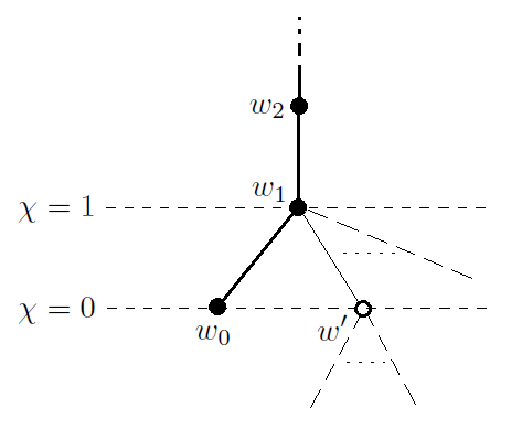
Figure 1. A sketch of a graded root with its main trunk. At least one vertex $w^{\prime}$ not on the main trunk is present on the 0-level, if the singularity is not rational.

4. The contact invariants: the Stein filling case

In this section, we prove Theorem 1.2 in the case where the minimal resolution $X_{min}$ has a good graph $\Gamma$. We build on ideas from [Ka, KO]: in these papers, Karakurt and Karakurt-Öztürk consider the case where the Heegaard Floer homology is isomorphic to $\mathbb{H}_{0}^{+}(\Gamma)$ (namely, they work with AR-graphs, for the definition see [Ne2, §8]), and study the image of the contact invariant $c^{+}(\xi)\in HF^{+}(-Y)$ in the lattice homology under this isomorphism. Even when the isomorphism no longer holds, we are able to apply a similar strategy.

First, we state a lemma for an arbitary negative-definite plumbing graph $\Gamma$ (the minimality assumption is not needed yet). Let $W(\Gamma)$ be the cobordism from $S^{3}$ to $Y=Y(\Gamma)$ given by the plumbing graph; $W(\Gamma)$ is obtained by cutting a small ball out of $X(\Gamma)$; $Spin^{c}$ structures on $W(\Gamma)$ are naturally identified with those on $X(\Gamma)$, and in turn with $\operatorname{Char}(\Gamma)$. We can think of $W(\Gamma)$ as cobordism from $-Y$ to $S^{3}$. Let $F^{+}_{W(\Gamma),\mathfrak{s}}:HF^{+}(-Y)\to HF^{+}(S^{3})$ be the map on Heegaard Floer homology induced by the $Spin^{c}$ cobordism $(W(\Gamma),\mathfrak{s})$ (see [OS4]). Following [OS2], define the map

$$T^{+}:HF^{+}(-Y)\to\mathbb{H}_{0}^{+}(\Gamma)$$

as follows: for $x\in HF^{+}(-Y)$, let $T^{+}(x):\operatorname{Char}(\Gamma)\to\mathcal{T}_{0}^{+}$ be given by

$$T^{+}(x)(K)=F^{+}_{W(\Gamma),\mathfrak{s}}(x)\in HF^{+}(S^{3})=\mathcal{T}_{0}^{+},$$

where $K$ is the element of $\operatorname{Char}$ associated with the $Spin^{c}$ structure $\mathfrak{s}$.

Lemma 4.1.

[OS2, Proposition 2.4] The map $T^{+}$ induces an $\mathbb{F}[U]$-equivariant map from $HF^{+}(-Y(\Gamma),\mathfrak{t})$ to $\operatorname{Hom}(\operatorname{Char}_{\mathfrak{t}}(\Gamma),\mathcal{T}_{0}^{+})$, whose image lies in $\mathbb{H}_{0}^{+}(\Gamma,\mathfrak{t})$.

Again, it’s important to note that the above lemma only uses basic properties of Heegaard Floer cobordism maps and requires no additional assumptions on the negative-definite graph $\Gamma$. (This map is an isomorphism for AR-graphs, see [Ne2, Theorem 8.3].)

We would like to find an explicit lattice-homological description of the element $c=T^{+}(c^{+}(\xi_{0}))\in\mathbb{H}_{0}^{+}(\Gamma)$. In the next lemma, we will do so under the additional assumption that the graph $\Gamma$ contains no $(-1)$ vertices, i.e. $X(\Gamma)$ is minimal and thus gives a Stein filling of $Y(\Gamma)$ (see Section 2). In the next section, we will expand the argument to the general case.

Lemma 4.2.

Assume that the graph $\Gamma$ contains no $(-1)$ vertices, i.e. $X(\Gamma)$ is Stein. Consider the element $c=T^{+}(c^{+}(\xi_{0}))\in\mathbb{H}_{0}^{+}(\Gamma)$. Let $K_{0}=c_{1}(TX,J)$. (1) The element $c$ is given by a function $\phi_{0}\in\mathbb{H}_{0}^{+}(\Gamma)$ such that $\phi_{0}(K_{0})=1$ in the degree $0$ part of $\mathcal{T}_{0}^{+}$ and $\phi_{0}(K)=0$ for any other characteristic class $K\neq K_{0}$. In particular, $c\in\mathbb{H}^{+}_{0}(\Gamma,[K_{0}])$.

(2) Under the isomorphism $i_{K_{0}}$ of Lemma 3.3, the function $\phi_{0}$ corresponds to the function $\varphi_{0}\in\mathbb{H}\mathbb{L}_{0}^{+}(\Gamma,K_{0})$ such that $\varphi_{0}(0)=1\in\mathcal{T}^{+}_{0}$ in degree $0$ and $\varphi_{0}(x)=0$ for any $x\neq 0$, $x\in L$.

(3) Under the isomorphism $\theta^{*}$ of Lemma 3.6, the function $\varphi_{0}$ corresponds to the function $\psi_{0}:\mathcal{V}(R_{K_{0}})\to\mathcal{T}_{0}^{+}$ such that $\psi_{0}(w_{0})$ is the generator of $\mathcal{T}_{0}^{+}$ in degree $0$, and $\psi_{0}=0$ for all other vertices of $R_{\mathfrak{t}_{can}}$. The vertex $w_{0}$ corresponds to the connected component of $0$ in the homology lattice.

Proof.

The argument is essentially the same as Karakurt’s observation in [Ka], based on the main theorem of [Pl]. Indeed, the homomorphism $c=T^{+}(c^{+}(\xi_{0}))$ is defined by

$$c(K)=F^{+}_{W(\Gamma),K}(c^{+}(\xi_{0}))\in HF^{+}(S^{3})=\mathcal{T}_{0}^{+}.$$

By [OS3], $c^{+}(\xi_{0})\in HF^{+}(Y,\mathfrak{s}_{can}|_{Y})$ , so it follows immediately that $c\in\mathbb{H}^{+}_{0}(\Gamma,[K_{0}])$ since the map $T^{+}$ respects $Spin^{c}$ structures.

By our assumption, $X(\Gamma)$ carries a Stein structure $J$ so that $(X,J)$ is a Stein filling for the canonical contact structure $\xi_{0}$ on $Y$. In this case [Pl, Theorem 4] asserts that $F^{+}_{W(\Gamma),\mathfrak{s}_{can}}(c^{+}(\xi_{0}))$ is the generator of $\mathcal{T}_{0}^{+}$ in degree $0$, and $F^{+}_{W(\Gamma),\mathfrak{s}}(c^{+}(\xi_{0}))=0$ for any other $Spin^{c}$-structure $\mathfrak{s}$ on $W(\Gamma)$. Since $c_{1}(\mathfrak{s}_{can})=c_{1}(TX,J)=K_{0}$ by our definition of the class $K_{0}$, this means that $c=\phi_{0}$.

Parts (2) and (3) of the lemma are immediate from the definitions of isomorphisms $\mathbb{H}_{0}^{+}(\Gamma,[K_{0}])\simeq\mathbb{H}\mathbb{L}_{0}^{+}(\Gamma,K_{0})\simeq\mathbb{H}(R_{K_{0}},\chi_{K_{0}})$ of Lemmas 3.3 and 3.6. ∎

Remark 4.3.

Under the hypothesis that $\Gamma$ contains no $(-1)$ vertices, the connected component $C_{0}$ of $0$ in the level set $\overline{L}_{K_{0},\leq 0}$ consists of a single point, ie $C_{0}=\{0\}$. Indeed, due to the isomorphism of Lemma 3.6, the function $\varphi_{0}$ must vanish on the entire component $C_{0}$. It is also easy to check that $C_{0}=\{0\}$ directly as follows. With the notation of Section 3.2, if $v$ is a basis element, we use the identity $\langle K_{0},v\rangle=v\cdot v+2$ to see that

$$\chi_{K_{0}}(x)-\chi_{K_{0}}(x\pm v)=\pm x\cdot v+\begin{cases}v\cdot v+1\textrm{\ or}\\ -1.\end{cases}$$

If $\Gamma$ has no $(-1)$ vertices, the inequality $v\cdot v\leq-2$ holds for any basis element $v$. Then for $x=0$, we get $\chi_{K_{0}}(0)=0$ but $\chi_{K_{0}}(\pm v)>0$ for any basis element $v$, so $0\in L$ is a single point in its connected component of the level set $\overline{L}_{K_{0},\leq 0}$.

In the next section, we examine the general case where $X(\Gamma)$ may not be Stein. We will see that Parts (1) and (2) of Lemma 4.2 no longer hold. However, it turns out that the zero set of the function $\varphi_{0}$ still matches the connected component $C_{0}$, so that Part (3) of Lemma 4.2 holds in general. See Section 5.

We now return to graded roots to establish a useful property of the function $\psi_{0}$.

Lemma 4.4.

Let $w_{0}$ be the distinguished vertex of the canonical graded root $(R_{K_{0}},\chi_{K_{0}})$ in the sense of Lemma 3.7. Consider $\psi_{0}:\mathcal{V}(R_{K_{0}})\to\mathcal{T}_{0}^{+}$ such that $\psi_{0}(w_{0})=1\in\mathcal{T}_{0}^{+}$ and $\psi_{0}(v)=0$ for all other vertices $v$ of $R_{K_{0}}$. Then $\psi_{0}\in\mathbb{H}(R_{K_{0}},\chi_{K_{0}})$, and $\psi_{0}\in\operatorname{Ker}U$. Moreover, $\psi_{0}\in\operatorname{Im}U$ if and only if the singularity is rational.

Proof.

We need to check that $\psi_{0}$ satisfies the compatibility conditions (4) which is immediate because the generator $1\in\mathcal{T}_{0}^{+}$ is annihilated by $U$ and by Lemma 3.7 part (1), there is no vertex $v$ of the graded root connected to $w_{0}$ such that $\chi(v)<\chi(w_{0})$ ($w_{0}$ is valency-one vertex of the graded root). Similarly, $\psi_{0}\in\operatorname{Ker}U$ follows from the relations (4). (Alternatively, one can use the fact that by Lemma 4.2 and Lemma 5.6, $\psi_{0}$ is the image of $c^{+}(\xi_{0})$ under the map from Heegaard Floer to lattice homology, and $c^{+}(\xi_{0})\in\operatorname{Ker}U$ in Heegaard Floer homology by [OS3].)

By [Ne2, Theorem 6.3], the singularity is rational if and only if $\mathbb{H}(R_{K_{0}},\chi_{K_{0}})=\mathcal{T}_{0}^{+}$, and this happens exactly when the graded root is a single infinite chain with the end vertex $w_{0}$, that is, the graded root consists of nothing else but the main trunk.

Therefore, if the singularity is rational, it is easy to see that $\psi_{0}\in\operatorname{Im}U$. If the singularity is not rational, the graded root $R_{K_{0}}$ has non-trivial branches, i.e., at least one vertex $v\neq w_{i}\ (i\in\mathbb{Z}^{+}_{0})$ outside its main trunk. Recall that $w_{1}$ is the (unique) vertex connected to $w_{0}$ by an edge in $R_{K_{0}}$ and $\chi_{K_{0}}(w_{1})=1$. By Lemma 3.7, all the vertices not on the main trunk must have non-positive $\chi_{K_{0}}$-value, so there exists a vertex $w^{\prime}\neq w_{0}$ such that $\chi(w^{\prime})=0$ and $w^{\prime}$ is connected to $w_{1}$, see Figure 1. Now, suppose that $\psi_{0}=U\psi$ for some $\psi\in\mathbb{H}(R_{K_{0}})$. Then $\psi(w_{1})=U\psi(w_{0})=\psi_{0}(w_{0})\neq 0$ and $\psi_{0}(w^{\prime})=U\psi(w^{\prime})=\psi(w_{1})\neq 0$, which is a contradiction because we defined $\psi_{0}(v)=0$ for all vertices $v\neq w_{0}$. ∎

Remark 4.5.

The above argument is similar to [KO, §5.8], but Karakurt-Öztürk in [KO] use Laufer sequences, an approach that only works in the special case of AR-singularities. Instead, we rely on the general graded root defined in [Ne2] for any negative definite rational homology sphere plumbed manifold.

Proof of Theorem 1.2.

The result follows immediately from Lemmas 4.4, 4.2, 4.1 in the Stein case. Similarly, in the general case the proof follows from Lemmas 4.4, 4.1, and Lemma 5.6 established in the next section. Indeed, for the canonical $Spin^{c}$ structure $\mathfrak{t}$ there is an $\mathbb{F}[U]$-equivariant map $HF^{+}(-Y(\Gamma),\mathfrak{t})\to\mathbb{H}_{0}^{+}(\Gamma,[K_{0}])\simeq\mathbb{H}\mathbb{L}_{0}^{+}(\Gamma,K_{0})\simeq\mathbb{H}(R_{K_{0}},\chi_{K_{0}})$ mapping $c^{+}(\xi_{0})$ to $\psi_{0}$. Therefore, if $\psi_{0}\notin\operatorname{Im}U$, then $c^{+}(\xi_{0})\notin\operatorname{Im}U$. ∎

5. The contact invariants in presence of blowups

In this section, we address the case where the minimal resolution $X_{min}\to\Sigma$ of the singularity $(\Sigma,0)$ does not have normal crossings. As discussed in Section 2, we can perform some additional blowups to obtain a normal crossing resolution $X=X(\Gamma)$, so that the resolution graph $\Gamma$ is good. The blowups are performed in several steps; at every step we blow up one or several points simultaneously. This gives a sequence of complex surfaces

$$X=X_{1}\to X_{2}\to X_{3}\to\dots X_{min}\to\Sigma,$$ (5)

where the maps are the corresponding blowdowns. It will be convenient, even if not strictly necessary, to assume that blowdowns are performed simultaneously whenever the surface contains several rational curves with self-intersection $-1$. (Note that in a surface with negative-definite intersection form, two distinct complex curves with self-intersection $-1$ must be disjoint.) The graph $\Gamma$ encodes the exceptional divisor of the composite map $X\to\Sigma$. If $\tilde{Z}\to Z$ is a blowup at a single point, we have $H_{2}(\tilde{Z})=H_{2}(Z)\oplus H_{2}(\overline{{\mathbb{CP}}^{2}})$, where the second summand corresponds to the exceptional divisor, and the map $H_{2}(Z)\hookrightarrow H_{2}(\tilde{Z})$ is induced by the inclusion of the punctured copy of $Z$ into $\tilde{Z}$. Thus, we have homology inclusions $H_{2}(X_{r})\hookrightarrow H_{2}(X)$ for each $r$.

We introduce notation for the components of the exceptional divisors at different stages of the blowup (5), as follows. Let $D^{1}_{1},D^{1}_{2},\dots,D^{1}_{k(1)}$ be the collection of disjoint rational curves of self-intersection $-1$ in $X_{1}$ that are blown down to obtain $X_{2}$, and let $E^{1}_{1},E^{1}_{2},\dots,E^{1}_{k(1)}$ denote the corresponding vertices of $\Gamma$. At the second step, there is a collection of disjoint exceptional curves $D^{2}_{1},D^{2}_{2},\dots,D^{2}_{k(2)}$ in $X_{2}$; these are simultaneously blown down to obtain $X_{3}$. Under the blowup $X_{1}\to X_{2}$, the strict transforms of $D^{2}_{1},D^{2}_{2},\dots,D^{2}_{k(2)}$ become components of the exceptional divisor in $X_{1}$ encoded by $\Gamma$, so they correspond to certain vertices $E^{2}_{1},E^{2}_{2},\dots,E^{2}_{k(2)}\in\Gamma$. (Under our assumption, $D^{2}_{j}$ could not be blown down in $X_{1}$, so $E^{2}_{j}\cdot E^{2}_{j}\leq-2$, and the self-intersection increases in $X_{2}$ as a result of the blowdown.) Inductively, we blow down a collection $D^{r}_{1},D^{r}_{2},\dots,D^{r}_{k(r)}$ of rational curves with self-intersection $-1$ in $X_{r}$ to obtain the surface $X_{r+1}$, until we arrive to the surface $X_{R+1}=X_{min}$ after $R$ steps. For each surface, we have a map $X\to X_{r}$ given by (5); for the divisors $D^{r}_{1},D^{r}_{2},\dots,D^{r}_{k(r)}\subset X_{r}$, their strict transforms in $X$ correspond to some components of the exceptional divisor of the map $X\to\Sigma$. This exceptional divisor is encoded by $\Gamma$; let $E^{r}_{1},E^{r}_{2},\dots,E^{r}_{k(r)}$ denote the vertices of $\Gamma$ that correspond to (the strict transforms of) $D^{r}_{1},D^{r}_{2},\dots,D^{r}_{k(r)}$.

Recall that the collection of divisors in $X$ corresponding to all vertices of the graph $\Gamma$ gives a basis of $H_{2}(X)$. Some, but not all, of these vertices appear in the sets $\{E^{r}_{1},E^{r}_{2},\dots,E^{r}_{k(r)}\}$ above. The vertices that do not appear in these sets correspond to classes that come from $H_{2}(X_{min})$.

Remark 5.1.

By construction, the smooth complex curve $D^{r}_{j}$ lies in $X_{r}$. Its preimage under the map $X\to\dots\to X_{r}$ is the total transform $\tilde{D}^{r}_{j}\subset X$; generally, this divisor is reducible. The image of the homology class of $D^{r}_{j}$ under the inclusion $H_{2}(X_{r})\hookrightarrow H_{2}(X)$ is the homology class of the total transform; we use the same notation $D^{r}_{j}$ for this class in $H_{2}(X)$. Note that when the total transform consists of several components and is not smooth, this class cannot be realized by a smooth complex curve in $X$: if $D$ were a smooth complex representative, then $D$ would non-negatively intersect all components of the total transform $\tilde{D}^{r}_{i}$, contradicting $D\cdot\tilde{D}^{r}_{i}=D\cdot D=-1$. By contrast, each class $D^{r}_{j}$ can be realized by a smooth symplectic sphere in $X$ with self-intersection $-1$, so that all these symplectic spheres (for all $r,j$) are pairwise disjoint. (Recall that the complex surface $X$ has a compatible symplectic structure $\omega_{0}$, see section 2.) Indeed, we start with the first blowup in $X_{min}$: for the map $X_{R}\to X_{min}=X_{R+1}$, the exceptional divisors $D^{R}_{1},D^{R}_{2},\dots,D^{R}_{k(R)}$ in $X_{R}$ are disjoint smooth complex (and thus symplectic) curves. Next, we blow up $X_{R}$ at one or more points to obtain $X_{R-1}$. If any of the blown-up points lie in the curves $D^{R}_{1},D^{R}_{2},\dots,D^{R}_{k(R)}$ in $X_{R}$, we can push each such divisor $D^{R}_{j}$ off these points by a $C^{\infty}$-small isotopy in $X_{R}$. Since being a symplectic surface is an $C^{\infty}$-open condition, the perturbed curves will be symplectic. These symplectic spheres are now unaffected by the blowups and thus remain smooth in $X_{R-1}$; they are obviously disjoint from the new exceptional divisors $D^{R-1}_{j}$ in $X_{R-1}$ (the curves $D^{R-1}_{j}$ are the preimages of the blown-up points under $X_{R-1}\to X_{R}$). We continue this process: before blowing up $X_{R-1}$ to get $X_{R-2}$, we perturb any of the affected spheres ($D^{R}_{j}$ or $D^{R-1}_{j}$) off the blown-up points, and so on, until we arrive at $X=X_{1}$ and a collection of disjoint symplectic spheres representing homology classes $D^{r}_{j}\in H_{2}(X)$ for all $r,j$.

Let

$$\mathcal{D}=\{D^{1}_{1},D^{1}_{2},\dots,D^{1}_{k(1)},D^{2}_{1},D^{2}_{2},\dots,D^{2}_{k(2)},\dots,D^{R}_{1},D^{R}_{2},\dots,D^{R}_{k(R)}\}\subset H_{2}(X)$$ (6)

be the set of homology classes $D^{m}_{j}$ in $X$ costructed above. Let $\mathcal{S}\subset H_{2}(X)$ be the set of sums $D_{i_{1}}+D_{i_{2}}+\dots+D_{i_{r}}$ of distinct elements from $\mathcal{D}$, where $\{D_{i_{1}},D_{i_{2}},\dots D_{i_{r}}\}$ ranges over subsets of $\mathcal{D}$. Note that $\mathcal{S}$ contains 0 (which corresponds to the empty subset). In other words,

$$\mathcal{S}=\{\sum_{n,i}\varepsilon^{n}_{i}D^{n}_{i}:D^{n}_{i}\in\mathcal{D},\varepsilon^{n}_{i}=0,1\}\subset H_{2}(X).$$ (7)

We will need to express the homology classes in $\mathcal{D}$ in terms of the basis elements $E^{n}_{i}\in H_{2}(X)$ corresponding to the vertices of $\Gamma$. It is convenient to use the notion of proximity (we tweak the usual definition of proximity of points to talk about proximity of divisors). Consider vertices $E^{a}_{i},E^{b}_{j}\in\Gamma$, with $b\geq a$. For the curve $E^{a}_{i}$ in $X=X_{1}$, we can consider its images under projection to the blowdown surfaces $X_{2},X_{3},\dots,X_{a}$. In $X_{a}$, the image is the curve $D^{a}_{i}$, it has self-intersection $(-1)$ and gets blown down at the subsequent step. Similarly, $E^{b}_{j}$ projects non-trivially to $X_{1},X_{2},\dots,X_{b}$ and becomes a point after the blowdown to $X_{b+1}$. If $D^{a}_{i}$ intersects the image of $E^{b}_{j}$ in $X_{a}$, we say that $E^{a}_{i}$ is proximate to $E^{b}_{j}$ and use notation $E^{a}_{i}\rightsquigarrow E^{b}_{j}$. Equivalently, $E^{a}_{i}\rightsquigarrow E^{b}_{j}$ if, once $E^{a}_{i}$ becomes a point in $X_{a+1}$ after the blowdown $X_{a}\to X_{a+1}$, this point lies in the image of $E^{b}_{j}$ in $X_{a+1}$. (Note that $E^{a}_{i}\rightsquigarrow E^{b}_{j}$ implies in fact that $b>a$: if $b=a$, then the projections of $E^{i}_{a}$ and $E^{b}_{j}$ to $X_{a}=X_{b}$ are the smooth complex curves $D^{a}_{i}$ and $D^{b}_{j}$ with self-intersection $(-1)$, which must be disjoint in a negative-definite manifold.)

Lemma 5.2.

The homology classes $D^{r}_{j}\in H_{2}(X)$ can be recursively expressed via the basis classes $E^{m}_{i}$ as follows:

$$D^{m}_{j}=E^{m}_{j}+\sum_{(i,n):E^{n}_{i}\rightsquigarrow E^{m}_{j}}D^{n}_{i}.$$ (8)

Proof.

The lemma follows from the familiar relation between the homology classes of the strict transform and the total transform. Indeed, blowing up $X_{m}$ to obtain $X_{m-1}$, we have

$$[\text{strict transform of }D^{m}_{j}\text{ in }X_{m-1}]=D^{m}_{j}-\sum_{i:E^{m-1}_{i}\rightsquigarrow E^{m}_{j}}D^{m-1}_{i},$$

because by definition, the proximate classes $E^{m-1}_{i}$ correspond precisely to exceptional divisors $D^{m-1}_{i}\subset X_{m-1}$ that project to points in $D^{m}_{j}$ under blowdown $X_{m-1}\to X_{m}$. Note that $D^{m}_{j}$ is a smooth complex curve in $X_{m}$, so all these points are smooth, and all the divisors enter with multiplicity 1 in the above formula for the strict transform.

Further, observe that the strict transform of $D^{m}_{j}$ in $X_{m-1}$ (taken with respect to the map $X_{m-1}\to X_{m}$) is the same as the projection of $E^{m}_{j}$ under the blowdown $X=X_{1}\to\dots\to X_{m-1}$. It follows that the vertices $E^{m-2}_{i}$ proximate to $E^{m}_{j}$ correspond exactly to those divisors $D^{m-2}_{i}$ among $D^{m-2}_{1},\dots,D^{m-2}_{k-2}$ in $X_{m-2}$ that project, under the blowdown $X_{m-2}\to X_{m-1}$, to points of this strict transform of $D^{m}_{j}$. All these points are smooth. Comparing the strict transform in $X_{m-2}$ to the total transform, we get

$$[\text{strict transform of }D^{m}_{j}\text{ in }X_{m-2}]=D^{m}_{j}-\sum_{i:E^{m-1}_{i}\rightsquigarrow E^{m}_{j}}D^{m-1}_{i}-\sum_{i:E^{m-2}_{i}\rightsquigarrow E^{m}_{j}}D^{m-2}_{i}.$$

We continue inductively, obtaining similar expressions for strict transforms of $D^{m}_{j}$ in $X_{m-3}$, etc, until we arrive at the formula for $E^{m}_{j}$, which is a strict transform of $D^{m}_{j}$ in $X=X_{1}$:

$$E^{m}_{j}=D^{m}_{j}-\sum_{(i,n):E^{n}_{i}\rightsquigarrow E^{m}_{j}}D^{n}_{i}.$$

∎

Explicit calculations (such as Example 5.3 below) can be done via handleslides on the plumbing graph, Kirby calculus-style. The graph $\Gamma$ gives a Kirby diagram for $X_{1}$ (each vertex corresponds to an unknotted component of the link). At each step of the blowdown, we look for $(-1)$-framed unknots in the diagram, handleslide them away, and blow down; the classes in $H_{2}$ corresponding to these $(-1)$ unknots in the diagram for $X_{r}$ are $D^{r}_{1},\dots,D^{r}_{k(r)}$. Proximity relation $E^{a}_{i}\rightsquigarrow E^{b}_{j}$ means that in the diagram for $X_{a}$, the $(-1)$-framed unknot representing $D^{a}_{i}$ is linked with the component that corresponds to $E^{b}_{j}$ (this component survives in $X_{a}$ because $b>a$). Accordingly, when we handleslide $D^{a}_{i}$ away from a link component, the homology class of the handle corresponding to the latter changes by adding $D^{a}_{i}$. It is not hard to see that in this context, Formula (8) is a consequence of handle addition operations and their effect on homology. Note that if we handleslide away the components corresponding to $D^{m}_{j}$ but do not blow them down, the resulting diagram represents $X$ at every step, and we explicitly see smooth representatives of the homology classes from $\mathcal{D}$ in $X$, given by all the $(-1)$ framed unknots that we slide away.

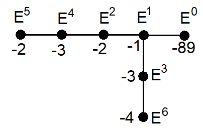
Figure 2. Plumbing graph of Example 5.3

Example 5.3.

Consider the negative definite plumbing graph of Figure 2. (This is the plumbing representation of the $(-1)$-surgery along the $(8,11)$ algebraic torus knot: the part of the graph obtained by deleting $E^{0}$ is the plumbing of $S^{3}$ arising as the embedded good resolution of the plane curve singularity $x^{8}=y^{11}$.)

In this example, at every blowdown step, we encounter one $(-1)$-divisor only, therefore, we omit the lower indices. The divisors $E^{1},E^{2},\dots,E^{6}$ can be blown down in this order consecutively. Just before $E^{1}$ is blown down, it intersects $E^{3}$ and $E^{2}$, so $E^{1}$ is proximate to $E^{3}$ and also to $E^{2}$. Next, $E^{2}$ is blown down, and just before this happens in $X_{1}$, it intersects the strict transforms of $E^{4}$ and $E^{3}$, so $E^{2}$ is proximate to $E^{4}$ and $E^{3}$. Similarly, $E^{3}$ is proximate to $E^{4}$ and $E^{6}$, $E^{4}$ is proximate to $E^{5}$ and $E^{6}$, and $E^{5}$ is proximate to $E^{6}$ only.

This means that we start with $D^{1}=E^{1}$. Then, since only $E^{1}$ is proximate to $E^{2}$, we have $D^{2}=D^{1}+E^{2}=E^{1}+E^{2}$. The divisors proximate to $E^{3}$ are $E^{2}$ and $E^{1}$, thus $D^{3}=D^{2}+D^{1}+E^{3}=2E^{1}+E^{2}+E^{3}$. Divisors $E^{3}$ and $E^{2}$ are proximate to $E^{4}$, so $D^{4}=D^{3}+D^{2}+E^{4}=3E^{1}+2E^{2}+E^{3}+E^{4}$. Only $E^{4}$ is proximate to $E^{5}$, so $D^{5}=D^{4}+E^{5}=3E^{1}+2E^{2}+E^{3}+E^{4}+E^{5}$. Divisors $E^{5},E^{4}$ and $E^{3}$ are all proximate to $E^{6}$: $D^{6}=D^{5}+D^{4}+D^{3}+E^{6}=8E^{1}+5E^{2}+3E^{3}+2E^{4}+E^{5}+E^{6}$. We will return to this example in the proof of Lemma 5.6.

We will now use the blowup formula in Heegaard Floer homology to identify the $Spin^{c}$ structures on $X$ with $F^{+}_{W(\Gamma),\mathfrak{s}}(c^{+}(\xi_{0}))\neq 0$. By contrast with Lemma 4.2, when $\Gamma$ has vertices of weight $-1$ it is no longer true that $F^{+}_{W(\Gamma),\mathfrak{s}}(c^{+}(\xi_{0}))=0$ for all $Spin^{c}$-structures $\mathfrak{s}$ other than the canonical one. Recall that $K_{0}=c_{1}(TX,J)$, and let $\mathfrak{s}_{min,can}$ denote the canonical $Spin^{c}$ structire on $X_{min}$.

Lemma 5.4.

Let $\mathfrak{s}$ be a $Spin^{c}$-structure on $X$.

(1) $F^{+}_{W,\mathfrak{s}}(c^{+}(\xi_{0}))$ is the generator of $\mathcal{T}_{0}^{+}$ in degree $0$ if $\langle c_{1}(\mathfrak{s}),D\rangle=\pm 1$ for all $D\in\mathcal{D}$, and $\mathfrak{s}|X_{min}=\mathfrak{s}_{min,can}$. Otherwise, $F^{+}_{W,\mathfrak{s}}(c^{+}(\xi_{0}))=0$.

(2) Equivalently, $F^{+}_{W,\mathfrak{s}}(c^{+}(\xi_{0}))=1\in\mathcal{T}_{0}^{+}$ if $c_{1}(\mathfrak{s})=K_{0}+2\operatorname{PD}(D)$ for some $D\in\mathcal{S}$; otherwise, $F^{+}_{W,\mathfrak{s}}(c^{+}(\xi_{0}))=0$.

Corollary 5.5.

(1) The element $c=T^{+}(c^{+}(\xi_{0}))\in\mathbb{H}_{0}^{+}(\Gamma)$ is given by the function $\phi_{0}\in\mathbb{H}_{0}^{+}(\Gamma)$ such that

$$\phi_{0}(\mathfrak{s})=\begin{cases}1\in\mathcal{T}_{0}^{+}\textrm{\ if\ }\mathfrak{s}=K_{0}+2\operatorname{PD}(D),D\in\mathcal{S},\\ 0\textrm{\ otherwise}.\end{cases}$$

(2) Under the isomorphism $i_{K_{0}}^{*}$ of Lemma 3.3, the function $\phi_{0}$ corresponds to the function $\varphi_{0}\in\mathbb{H}\mathbb{L}_{0}^{+}(\Gamma,K_{0})$ such that for $x\in L$,

$$\varphi_{0}(x)=\begin{cases}1\in\mathcal{T}_{0}^{+}\textrm{\ if\ }x\in\mathcal{S},\\ 0\textrm{\ otherwise}.\end{cases}$$

Proof of Corollary 5.5.

This follows from Lemma 5.4, by an argument completely analogous to the proof of Lemma 4.2 ∎

.

Proof of Lemma 5.4.

(1) In the minimal case, the set $\mathcal{S}$ is empty, and the statement was already given in Lemma 4.2.

In the non-minimal case, we blow down $X$ to $X_{min}$, perhaps in several steps, and argue by induction on the number of exceptional divisors in this sequence of blowdowns.

Suppose the statement holds for the complex surface $X^{\prime}$ which is a blowup of $X_{min}$, and $X$ is obtained from $X^{\prime}$ by an additional blowup with exceptional divisor $D_{0}$. Let $\mathcal{D}^{\prime}$ and $\mathcal{S}^{\prime}$ be the sets of homology classes defined for $X^{\prime}$ as in formulas (6) and (7). Note that $H_{2}(X)=H_{2}(X^{\prime})\oplus\mathbb{Z}$; identifying homology classes in $X^{\prime}$ with their images under inclusion in $X$, we have $\mathcal{D}=\mathcal{D}^{\prime}\cup\{D_{0}\}$. Let $W$, $W^{\prime}$ denote the corresponding cobordisms from $-Y^{3}$ to $S^{3}$, and let $B=[0,1]\times Y\#\overline{{\mathbb{CP}}^{2}}$ be the blowup cobordism. As a smooth manifold, $W$ can be thought of as composition of cobordism $B$ from $-Y$ to $-Y$ followed by cobordism $W^{\prime}$ from $-Y$ to $S^{3}$. Since $W=W^{\prime}\#\overline{{\mathbb{CP}}^{2}}$, a $Spin^{c}$-structure $\mathfrak{s}$ on $W$ is completely determined by its restrictions $\mathfrak{s}|_{W^{\prime}}$ and $\mathfrak{s}|_{B}$, so by the composition law [OS4, Theorem 3.4], we have

$$F^{+}_{W^{\prime},\mathfrak{s}|_{W^{\prime}}}\circ F^{+}_{B,\mathfrak{s}|B}=F^{+}_{W,\mathfrak{s}}.$$

We are interested in the canonical contact structure $\xi_{0}$ on $Y=\partial X^{\prime}=\partial X$, so we focus on $Spin^{c}$-structures with $\mathfrak{s}|_{Y}=\mathfrak{s}_{can}|_{Y}$, since $c^{+}(\xi_{0})\in HF^{+}(Y,\mathfrak{s}_{can}|_{Y})$.

The map $F^{+}_{B,\mathfrak{s}|B}$ is given by the Ozsváth–Szabó blowup formula [OS4, Theorem 3.7]. Let $D_{0}$ be the exceptional divisor of the blowup, and $\langle c_{1}(\mathfrak{s}),D_{0}\rangle=\langle c_{1}(\mathfrak{s}|B),D_{0}\rangle=\pm(2l+1)$, $l\geq 0$. Then

$$F^{+}_{B,\mathfrak{s}|B}:HF^{+}\left({-Y,\mathfrak{s}|_{Y}}\right)\to HF^{+}\left({-Y,\mathfrak{s}|_{Y}}\right)$$

is the multiplication by $U^{l(l+1)}$. By [OS3], the contact invariant lies in $\operatorname{Ker}U$, thus we get we get $F^{+}_{B,\mathfrak{s}|B}(c^{+}(\xi_{0}))=0$ if $l\neq 0$. For $l=0$, $F^{+}_{B,\mathfrak{s}|B}(c^{+}(\xi_{0}))=c^{+}(\xi_{0})$ since $F^{+}_{B,\mathfrak{s}|B}$ is the identity map.

By the induction hypothesis, $F^{+}_{W^{\prime},\mathfrak{s}|_{W^{\prime}}}(c^{+}(\xi_{0}))$ is the generator $1\in\mathcal{T}_{0}^{+}$ if $\mathfrak{s}|_{W_{min}}=\mathfrak{s}_{min,can}$ and $\langle c_{1}(\mathfrak{s}),D^{\prime}\rangle=\pm 1$ for all $D^{\prime}\in\mathcal{D}^{\prime}$; moreover, $F^{+}_{W^{\prime},\mathfrak{s}|_{W^{\prime}}}(c^{+}(\xi_{0}))$ is zero for all other $Spin^{c}$ structures. Then from the composition formula, $F^{+}_{W,\mathfrak{s}|_{W}}(c^{+}(\xi_{0}))=1\in\mathcal{T}_{0}^{+}$ if

$$\mathfrak{s}|_{W_{min}}=\mathfrak{s}_{min,can},\quad\langle c_{1}(\mathfrak{s}),D^{\prime}\rangle=\pm 1\text{ for all }D^{\prime}\in\mathcal{D}^{\prime},\text{ and }\langle c_{1}(\mathfrak{s}),D_{0}\rangle=\pm 1.$$

For all other $Spin^{c}$ structures on $X$, $F^{+}_{W,\mathfrak{s}}(c^{+}(\xi_{0}))=0$. Since $\mathcal{D}=\mathcal{D^{\prime}}\cup\{D_{0}\}$, part (1) of the lemma holds for $Spin^{c}$ structures on $X$.

(2) Observe that for a $Spin^{c}$-structure $s$ with $\mathfrak{s}|_{W_{min}}=\mathfrak{s}_{can}$ and $\langle c_{1}(\mathfrak{s}),D\rangle=\pm 1$ for all $D\in\mathcal{D}$, we have

$$c_{1}(\mathfrak{s})=c_{1}(\mathfrak{s}_{can,W_{min}})+\sum_{m,j}\pm\operatorname{PD}(D^{m}_{j}).$$

The canonical $Spin^{c}$ structure $\mathfrak{s}_{can}$ on $W$ is determined by the equalities $\mathfrak{s}|_{W_{min}}=\mathfrak{s}_{can,W_{min}}$ and $\langle c_{1}(\mathfrak{s}),D^{m}_{j}\rangle=+1$ for all $D^{m}_{j}\in\mathcal{D}$, so

$$K_{0}=c_{1}(\mathfrak{s}_{can})=c_{1}(\mathfrak{s}_{can,W_{min}})-\sum_{m,j}\operatorname{PD}(D^{m}_{j}).$$

The statement now follows from the first part of the lemma. ∎

We now show that part (3) of Lemma 4.2 holds in the general case even though parts (1) and (2) don’t. Corollary 5.5 identifies the zero set of the function $\varphi_{0}$ as the set $\mathcal{S}\subset H_{2}(X;\mathbb{Z})$ given by sums of distinct homology classes from $\mathcal{D}$. To understand the function $\psi_{0}$ corresponding to $\varphi_{0}$ in the graded root description of lattice homology, we examine connected components of the level set $\overline{L}_{K_{0},\leq 0}$ (compare with Remark 4.3).

Lemma 5.6.

(1) Let $C_{0}$ be the connected component of $0$ in the level set $\overline{L}_{K_{0},\leq 0}$. Then $\mathcal{S}$ is contained in $C_{0}$. (In fact, $\mathcal{S}=C_{0}$.)

(2) Under the isomorphism $\theta^{*}$ of Lemma 3.6, the function $\varphi_{0}$ corresponds to the function $\psi_{0}:\mathcal{V}(R_{K_{0}})\to\mathcal{T}_{0}^{+}$ such that $\psi_{0}(w_{0})$ is the generator of $\mathcal{T}_{0}^{+}$ in degree $0$, and $\psi_{0}=0$ for all other vertices of $R_{\mathfrak{t}_{can}}$. The vertex $w_{0}$ corresponds to the connected component of $0$ in the homology lattice.

Proof.

(1) We saw that the homology classes $D^{m}_{j}$ in the set $\mathcal{D}$ can be represented by pairwise disjoint symplectic spheres of self-intersection $(-1)$ in $X=X_{0}$. It follows that these classes all lie in the zero level set of $\chi_{K_{0}}$: by adjunction formula, $\langle K_{0},D^{m}_{j}\rangle=\langle c_{1}(TX,J),D^{m}_{j}\rangle=D^{m}_{j}\cdot D^{m}_{j}+2=1$, therefore,

$$\chi_{K_{0}}(D^{m}_{j})=0.$$

Clearly, $D^{m}_{j}\cdot D^{n}_{i}=0$ for any two distinct classes since they have disjoint representatives. The property of the weight function $\chi_{K_{0}}(x+y)=\chi_{K_{0}}(x)+\chi_{K_{0}}(y)-x\cdot y$ then implies that $\chi_{K_{0}}=0$ for any of the sums forming $\mathcal{S}$, thus $\mathcal{S}$ lies in the zero level set $\overline{L}_{K_{0},\leq 0}$. It will be convenient to refer to $D^{m}_{1},D^{m}_{2},\dots,D^{m}_{k(m)}$ as elements of depth $m$, $1\leq m\leq R$.

We want to show that $\mathcal{S}$ lies in the connected component $C_{0}$. Recall from section 3.2 that 1-cells in $\overline{L}_{K_{0},\leq 0}$ correspond to basis vectors in the lattice $L=H_{2}(X,\mathbb{Z})$: we can walk from $x\in L$ to $x+v\in L$ along the edge corresponding to $v$ if $v$ is a basic vector. For each element of depth 1, the homology class $D^{1}_{i}=E^{1}_{i}$ is in the basis, thus $D^{1}_{i}=0+E^{1}_{i}$ lies in $C_{0}$ because it is connected to 0 by the egde corresponding to $E^{1}_{i}$. A typical lattice point $F\in\mathcal{S}$ is a sum of some elements $D^{m}_{j}$. We will show that $F\in C_{0}$ recursively, by reducing to sums of elements of lower depth. The key idea is Formula (8), which recursively expresses classes $D^{m}_{j}$ in terms of the basis elements $E^{1}_{1},\dots,E^{R}_{k(R)}$. Notice that in the above formula, each instance of $n$ on the right hand side is strictly less than $m$, thus $D^{m}_{j}=E^{m}_{j}+\text{sum of elements of lower depth}$.

First, we illustrate the recursive procedure for the lattice from Example 5.3. In fact, we construct the paths from 0 starting with elements of lower depth and building up to higher depth; the recursion will work backwards, reducing the depth. To begin, observe that $D^{1}\in C_{0}$ as above. Next, $D^{2}=D^{1}+E^{2}$ is one step away from $D^{1}$ along the edge $E^{2}$, so $D^{2}\in C_{0}$. Further, $D^{1}+D^{2}=D^{2}+E^{1}$ is connected to $D^{2}$ by the edge $E^{1}$, so $D^{1}+D^{2}\in C_{0}$. Next, we see that $D^{3}=D^{1}+D^{2}+E^{3}$ is connected to the vertex $D^{1}+D^{2}\in C_{0}$ by the edge $E^{3}$, so $D^{3}\in C_{0}$. Then, we establish that $D^{1}+D^{3}=D^{3}+E^{1}\in C_{0}$, and then $D^{2}+D^{3}=D^{3}+D^{1}+E^{1}\in C_{0}$, and then $D^{1}+D^{2}+D^{3}=D^{2}+D^{3}+E^{1}\in C_{0}$. Now we see that $D^{4}=D^{2}+D^{3}+E^{4}\in C_{0}$ because we already know that $D^{2}+D^{3}\in C_{0}$. We can write out the full path from 0 to $D^{4}$:

$$D^{4}=\underbrace{\underbrace{\underbrace{E^{1}}_{D^{1}}+E^{2}}_{D^{2}}+\underbrace{E^{1}}_{D^{1}}+E^{3}}_{D^{3}}+\underbrace{\underbrace{E^{1}}_{D^{1}}+E^{2}}_{D^{2}}+E^{4}.$$

In this form, $D^{4}=\sum_{j=1}^{k}E^{i(j)}$ (with possibly repeating indices $i(j)$) is the sum of basis elements, showing steps along the corresponding edges. The initial partial sums $P^{m}=\sum_{j=1}^{m}E^{i(j)}$ we obtain after each step correspond to the vertices of the lattice $L$ that our path goes through, starting from 0. The underbraces show that each such vertex is a sum of some distinct elements $D^{j}$. All of these sums lie in $\mathcal{S}$ which is contained the level set $\overline{L}_{K_{0},\leq 0}$, thus we see that all the lattice points on the path lie in $\overline{L}_{K_{0},\leq 0}$, showing that the entire path lies in the connected component of 0.

We continue in this fashion, consecutively building paths to elements $D^{4}+D^{1}$, $D^{4}+D^{2}$, $D^{4}+D^{2}+D^{1}$, $D^{4}+D^{3}$, $D^{4}+D^{3}+D^{1}$ etc, until we reach all elements in $\mathcal{S}$. Here is the recursively constructed full path showing that $D^{6}$ is in the connected component of $0$:

$$\underbrace{\underbrace{\underbrace{\underbrace{\underbrace{E^{1}}_{D^{1}}+E^{2}}_{D^{2}}+\underbrace{E^{1}}_{D^{1}}+E^{3}}_{D^{3}}+\underbrace{\underbrace{E^{1}}_{D^{1}}+E^{2}}_{D^{2}}+E^{4}}_{D^{4}}+E^{5}}_{D^{5}}+\underbrace{\underbrace{\underbrace{\underbrace{E^{1}}_{D^{1}}+E^{2}}_{D^{2}}+\underbrace{E^{1}}_{D^{1}}+E^{3}}_{D^{3}}+\underbrace{\underbrace{E^{1}}_{D^{1}}+E^{2}}_{D^{2}}+E^{4}}_{D^{4}}+$$

$$+\underbrace{\underbrace{\underbrace{E^{1}}_{D^{1}}+E^{2}}_{D^{2}}+\underbrace{E^{1}}_{D^{1}}+E^{3}}_{D^{3}}+E^{6}=D^{6}.$$

We now return to the proof of Lemma 5.6 and proceed with the formal recursion. To every lattice point $F\in\mathcal{S}$ we can assign an $R$-tuple of integers

$$t(F):=(s_{R},\dots,s_{2},s_{1}),$$

where $s_{r}$ is the number of summands in $F$ that are elements of depth $r$. Namely, if $F=\sum_{a,i}\varepsilon^{a}_{i}D^{a}_{i}$, $\varepsilon^{a}_{i}\in\{0,1\},D^{a}_{i}\in\mathcal{D}$, we set $s_{r}:=\sum_{i=1}^{k(r)}\varepsilon^{r}_{i}$, $1\leq r\leq R$.

We define a partial ordering on $\mathcal{S}$ as follows. For $F_{1},F_{2}\in\mathcal{S}$ we say that $F_{1}\prec F_{2}$ if $t(F_{1})<t(F_{2})$ with respect to the lexicographical ordering, looking for the first differing number from the left (the largest index $r$ where there is no equality). In other words, $F_{1}\prec F_{2}$ if $F_{1}$ has fewer elements of depth $r$ than $F_{2}$, and $F_{1}$ and $F_{2}$ have the same number of elements of depth $r+1,r+2,\dots,R$.

Take any element $F\in\mathcal{S}$. Let $u$ be the smallest upper index among the summands of $F$, and write $F$ in the form $F=\overline{F}+D^{u}_{i}$, where all summands in $\overline{F}$ have upper index at least $u$ ($\overline{F}$ might be an empty sum). Looking at Formula (8), we get $D^{u}_{i}=\overline{D}+E^{u}_{i}$, where all summands $\overline{D}\in\mathcal{F}_{u-1}$ have upper index less than $u$. Again, $\overline{D}$ might be an empty sum.

It follows that $\overline{F}$ and $\overline{D}$ cannot share any summands, so the sum $\widetilde{F}=\overline{F}+\overline{D}$ lies in $\mathcal{S}$. Moreover, due to our choice of the index $u$, we have $\widetilde{F}\prec F$. Because $F=\widetilde{F}+E^{u}_{i}$, this shows that any nontrivial element of $\mathcal{S}$ can be written as a sum of a lexicographically lower element and a basis element. To illustrate, we would decompose the element $F=D^{4}+D^{3}$ in the above example as $F=\widetilde{F}+E^{3}$, where $\widetilde{F}=D^{4}+D^{2}+D^{1}$ is lexicographically lower than $F$; similarly, $D^{4}+D^{2}+D^{1}=D^{4}+D^{2}+E^{1}$, with $D^{4}+D^{2}\prec D^{4}+D^{2}+D^{1}$.

The relation $F=\widetilde{F}+E^{u}_{i}$ implies that $F$ is connected to $\widetilde{F}$ by the edge $E^{u}_{i}$. Therefore, if $\widetilde{F}$ is in the connected component $C_{0}$, then so is $F$. Since the empty sum equals 0 and obviously lies in $C_{0}$, the above recursion shows that every element of $\mathcal{S}$ is in $C_{0}$.

It is worth noting that the above decomposition $F=\widetilde{F}+E^{u}_{i}$ provides a recursive way to write any sum from $\mathcal{S}$ as a series of basis elements, indicating the path starting at zero and ending at the given lattice point, as shown in the example above.

We have shown that $\mathcal{S}\subset C_{0}$. Corollary 5.5 identifies $\mathcal{S}$ with the zero set of $\varphi_{0}$. The proof of Lemma 3.6 implies that that the zero set of the function $\varphi_{0}$ is the union of several connected components of $\overline{L}_{K_{0},\leq 0}$ (in particular, $\varphi_{0}$ must vanish on entire connected components). It follows that $\mathcal{S}=C_{0}$.

(2) The second statement of the lemma follows from the first statement, Corollary 5.5, and Lemma 3.6. (Compare with Part (3) of Lemma 4.2.) ∎

Remark 5.7.

In this paper we worked with coefficients in $\mathbb{F}=\mathbb{Z}/2$ for simplicity, however our results hold for integer coefficients as well. When working with $\mathbb{Z}$ coefficients, the contact invariant $c^{+}(\xi)$ is only defined up to sign. The results of [Pl, Ghi] then assert that $F^{+}_{W(\Gamma),\mathfrak{s}_{can}}(c^{+}(\xi))$ is a generator $\pm 1\in\mathcal{T}_{0}^{+}$, where $\mathcal{T}_{0}^{+}$ now stands for $\mathbb{Z}[U,U^{-1}]/U\cdot\mathbb{Z}[U]$. A further issue is that cobordism maps are only defined up to sign in [OS4], although [OS2, §2.1] explains how to define the map $T^{+}$ up to one overall sign (which can also be fixed). The isomorphisms between various constructions of lattice cohomology work with $\mathbb{Z}$ coefficients, and the distinguished elements $\phi_{0}$, $\varphi_{0}$, and $\psi_{0}$ of Lemma 4.2 and its analogs in Section 5 correspond to one another. Thus, we see that the element $c^{+}(\xi_{0})\in HF^{+}(-Y(\Gamma),\mathfrak{t})/\pm 1$ is mapped to $(\pm\psi_{0})$ under the map $HF^{+}(-Y(\Gamma),\mathfrak{t})/\pm 1\to\mathbb{H}(R_{K_{0}},\chi_{K_{0}})/\pm 1$, and our proof goes through as before.

References

- [BO] F. Bogomolov and B. de Oliveira, Stein small deformations of strictly pseudoconvex surfaces, Birational algebraic geometry (Baltimore, MD, 1996), 25–41, Contemp. Math., 207, AMS, Providence, RI, 1997.
- [CNP] C. Caubel, A. Némethi, P. Popescu-Pampu, Milnor open books and Milnor fillable contact 3-manifolds, Topology 45 (2006), no. 3, 673–689.
- [Elk] R. Elkik, Singularités rationelles et Déformations, Inv. Math. 47 (1978), 139–147.
- [Ghi] P. Ghiggini, Ozsváth–Szabó invariants and fillability of contact structures, Math. Zeit. 253 (2006), no. 1, 159–175.
- [GS] R. Gompf, A. Stipsicz, 4-manifolds and Kirby calculus, AMS, Providence, RI, 1999.
- [Ha] R. Hartshorne, Algebraic Geometry, Springer, 1977.
- [Ka] C. Karakurt, Contact structures on plumbed 3-manifolds, Kyoto J. Math. 54 (2014), no. 2, 271–294.
- [KO] C. Karakurt, F. Öztürk, Contact Structures on AR-singularity links, arXiv:1702.06371.
- [LO] Y. Lekili, B. Ozbagci, Milnor fillable contact structures are universally tight, Math. Res. Lett. 17 (2010), no. 6, 1055–1063.
- [Ne1] A. Némethi, Five lectures on normal surface singularities, in: Bolyai Society Mathematical Studies 8, Low Dimensional Topology, 269–351, 1999.
- [Ne2] A. Némethi, On the Oszváth–Szabó invariant of negative definite plumbed 3-manifolds, Geom. Topol. 9 (2005), 991–1042.
- [Ne3] A. Némethi, Lattice cohomology of normal surface singularities, Publ. RIMS. Kyoto Univ., 44 (2008), 507–543.
- [Ne4] A. Némethi, Links of rational singularities, L-spaces and LO fundamental groups, Invent. Math., 210 (2017), no. 1, 69–83.
- [LN] T. László, A. Némethi, Reduction theorem for lattice cohomology, Int. Math. Res. Not. 11 (2015), 2938–2985.
- [OS1] P. Ozsváth and Z. Szabó, Holomorphic disks and topological invariants for closed 3-manifolds, Ann. of Math. (2) 159 (2004), no. 3, 1027–1158.
- [OS2] P. Ozsváth, Z. Szabó, On the Floer homology of plumbed three-manifolds, Geom. Topol. 7 (2003), 185–224.
- [OS3] P. Ozsváth, Z. Szabó, Heegaard Floer homologies and contact structures, Duke Math. J. 129 (2005), no. 1, 39–61.
- [OS4] P. Ozsváth, Z. Szabó, Holomorphic triangles and invariants for smooth four-manifolds, Adv. Math. 202 (2006) no. 2, 326–400.
- [OSS] P. Ozsváth, A. Stipsicz, Z. Szabó, A spectral sequence on lattice homology, Quantum Topol. 5 (2014), 487–521.
- [Pl] O. Plamenevskaya, Contact structures with distinct Heegaard Floer invariants, Math. Res. Lett. 11 (2004), no. 4, 547–561.