OGLE-2017-BLG-0039: Microlensing Event with Light from the Lens Identified from Mass Measurement

Abstract

We present the analysis of the caustic-crossing binary microlensing event OGLE-2017-BLG-0039. Thanks to the very long duration of the event, with an event time scale $t_{\rm E}\sim 130$ days, the microlens parallax is precisely measured despite its small value of $\pi_{\rm E}\sim 0.06$. The analysis of the well-resolved caustic crossings during both the source star’s entrance and exit of the caustic yields the angular Einstein radius $\theta_{\rm E}\sim 0.6$ mas. The measured $\pi_{\rm E}$ and $\theta_{\rm E}$ indicate that the lens is a binary composed of two stars with masses $\sim 1.0~{}M_{\odot}$ and $\sim 0.15~{}M_{\odot}$, and it is located at a distance of $\sim 6$ kpc. From the color and brightness of the lens estimated from the determined lens mass and distance, it is expected that $\sim 2/3$ of the $I$-band blended flux comes from the lens. Therefore, the event is a rare case of a bright lens event for which high-resolution follow-up observations can confirm the nature of the lens.

1. Introduction

It is believed that most microlensing events detected toward the Galactic bulge field are produced by stars (Han & Gould, 2003). For stellar lens events, the observed light comes from the lens as well as from the source star. However, lenses, in most cases, are much fainter than the source stars being monitored, and thus it is difficult to detect the light from the lens. In some rare cases for which the lenses are bright, the light from the lens can be detected. However, even in such cases, it is still difficult to attribute the excess flux to the lens because the flux may come from nearby stars blended in the image of the source or possibly from the companion to the source if the source is a binary.

Figure 1.— Light curve of OGLE-2017-BLG-0039. The curve superposed on data points represents the best-fit binary lens model (close binary solution with $u_{0}>0$). The lower panel shows the residual from the model.

There have been several methods proposed to identify light from lenses. The most explicit method is resolving the lens from the source or other blended stars from high-resolution follow-up observations. For typical lensing events, the relative lens-source proper motions is $\mu\sim 5$ mas yr^-1. This means that one has to wait $\sim 10$ – 20 years for direct lens imaging until the lens is separated enough from the source even using the currently available instrument with the highest resolution (Han & Chang, 2003). As a result, the method has been applied to only 3 lensing events: MACHO-LMC-5 (Alcock et al., 2001), MACHO-95-BLG-37 (Kozłowski et al., 2007), and OGLE-2005-BLG-169 (Batista et al., 2015; Bennett et al., 2015).

A bright lens can also be identified from astrometric observations of lensing events. When a source star is gravitationally lensed, the centroid of the source star image is displaced from the position of the unlensed source star (Høg et al., 1995; Miyamoto & Yoshii, 1995; Paczyński, 1998; Boden et al., 1998). Due to the relative lens-source motion, the position of the image centroid traces out an elliptical trajectory where the size and shape of the trajectory are determined by the angular Einstein radius and the impact parameter of the lens-source approach (Walker, 1995; Jeong et al., 1999). If an event is produced by a bright lens, the astrometric shift is affected by the light from the lens and one can identify the bright lens from the deviation (Han & Jeong, 1999). Lensing-induced astrometric shifts produced by very nearby stars have been measured, e.g., Stein 2051 B (Sahu et al., 2017) and Proxima Centauri (Zurlo et al., 2018). For general lensing events, however, it is currently difficult to measure image motions due to the required high accuracy of an order 10 $\mu$as.

In some limited cases, a bright lens can also be identified from the analysis of the lensing light curve obtained from photometric observations. This photometric identification is possible for events where the mass $M$ and distance $D_{\rm L}$ to the lens are determined. With the determined $M$ and $D_{\rm L}$, one can predict the color and brightness of the lens. If the color and brightness are close to those of the blend, then, it is likely that the flux from the lens comprises an important portion of the total blended flux. Due to the bright nature of the lens, the lens will be visible in high-resolution images, which are obtained from space-based or ground-based adaptive optic (AO) observations, as an additional light that is blended with the source image (Bennett et al., 2007). Then, one can identify the lens by comparing the excess flux with the prediction from lensing modeling. Bright lenses have been identified by space-based follow-up observations using Hubble Space Telescope for the first two planetary microlensing events OGLE-2003-BLG-235 (Bond et al., 2004) and OGLE-2005-BLG-071 (Udalski et al., 2005) by Bennett et al. (2006) and Dong et al. (2009), respectively. For OGLE-2006-BLG-109 (Gaudi et al., 2008; Bennett et al., 2010) and OGLE-2012-BLG-0026 (Han et al., 2013), for which multiple microlensing planetary systems were found, the light from the lenses were confirmed by Keck AO follow-up observations conducted by Bennett et al. (2010) and Beaulieu et al. (2016), respectively.

For various reasons, long time-scale binary-lens events are ideal targets in applying the photometric method of bright lens identification. First, the chance to determine the lens mass and distance is high for these events. For the determinations of $M$ and $D_{\rm L}$, it is required to measure both the microlens parallax $\pi_{\rm E}$ and the angular Einstein radius $\theta_{\rm E}$, which are related to $M$ and $D_{\rm L}$ by

$$M={\theta_{\rm E}\over\kappa\pi_{\rm E}}$$ (1)

and

$$D_{\rm L}={{\rm au}\over\pi_{\rm E}\theta_{\rm E}+\pi_{\rm S}}$$ (2)

respectively (Gould, 2000). Here $\kappa=4G/(c^{2}{\rm au})$, $\pi_{\rm S}={\rm au}/D_{\rm S}$ is the parallax of the source star, and $D_{\rm S}$ denotes the distance to the source. We note that $\pi_{\rm S}$ is known for events detected toward the Galactic bulge direction because source stars are located in the bulge and thus $D_{\rm S}$ is known. The angular Einstein radius is measured from the deviation in lensing light curves affected by finite-source effects. For single-lens events, finite-source effects can be detected only for very rare events in which the lens passes over the surface of the source star, e.g., Choi et al. (2012), and thus the chance to measure $\theta_{\rm E}$ is low. For binary-lens events, in contrast, the chance to measure $\theta_{\rm E}$ is high because these events usually accompany caustic-crossing features in lensing light curves from which one can measure $\theta_{\rm E}$. The chance to measure $\pi_{\rm E}$ is also high for these events due to their long time scales. As an event time scale approaches or exceeds the orbital period of Earth, i.e., 1 yr, the relative lens-source motion deviates from rectilinear due to the acceleration of the observer’s motion caused by the Earth’s orbital motion. The deviation in the relative lens-source motion results in lensing light curve deviations from which one can measure the microlens parallax (Gould, 1992). Being able to measure both $\theta_{\rm E}$ and $\pi_{\rm E}$, the chance to measure the physical lens parameters of $M$ and $D_{\rm L}$ is high for long time-scale binary-lens events. Second, the chance for these events to be produced by bright lenses is higher. This is because the event time scale is proportional to the square root of the lens mass, i.e., $t_{\rm E}\propto\sqrt{M}$, and thus the lens mass tends to be heavier and brighter than general events with $t_{\rm E}\sim(O)10$ days. As the lens becomes brighter, the fraction of the lens flux in the total blended flux increases, making it easier to identify the bright lens.

In this work, we present the analysis of the binary-lens event OGLE-2017-BLG-0039. The event has a very long time scale with well-resolved caustic-crossing features in the light curve. Being able to determine the lens mass and distance by simultaneously measuring both $\pi_{\rm E}$ and $\theta_{\rm E}$, we check the lens origin of the blended light.

2. Observations

The microlensing event OGLE-2017-BLG-0039 occurred on a star located toward the Galactic bulge field. The coordinates of the source star are $({\rm RA},{\rm DEC})_{\rm J2000}=$ (18:01:47.95, -27:20:34.7), which corresponds to the galactic coordinates $(l,b)=(3.18^{\circ},-2.27^{\circ})$. The apparent baseline brightness before lensing magnification was $I_{\rm base}\sim 19.1$.

The lensing-induced brightening of the source star was found and alerted by the Early Warning System of the Optical Gravitational Lensing Experiment (OGLE; Udalski et al., 2015) survey on 2017 February 14 (${\rm HJD}^{\prime}={\rm HJD}-2450000\sim 7798$). The OGLE survey was conducted using the 1.3 m Warsaw Telescope located at the Las Campanas Observatory in Chile. The event was in the OGLE BLG511.23 field, toward which observations were carried out 3 – 10 times per night. Images were taken primarily in $I$ band and $V$-band images were occasionally obtained for the color measurement of the source star. Photometry of the images is extracted using the OGLE difference-imaging pipeline (Udalski, 2003).

The event was also in the fields that were observed by the Microlensing Observations in Astrophysics (MOA: Bond et al., 2001) and the Korea Microlensing Telescope Network (KMTNet: Kim et al., 2016) surveys. MOA observations were conducted in a customized $R$ band using the 1.8 m telescope of the Mt. John University Observatory in New Zealand. The event was dubbed MOA-2017-BLG-080 in the list of MOA transient events. About 10 images were taken each night from the MOA survey. KMTNet observations of the event were conducted using three identical 1.6 m telescopes that are globally distributed at the Cerro Tololo Interamerican Observatory, Chile (KMTC), the South African Astronomical Observatory, South Africa (KMTS), and the Siding Spring Observatory, in Australia (KMTA). Most KMTNet data were taken in $I$ band, and some $V$-band images were acquired for the source color measurement. The event is in the KMTNet BLG03 field for which observations were conducted at a cadence of 2 per hour. Most of the BLG03 field is additionally covered by the BLG43 field with a slight offset in order to cover the gaps between CCD chips as well as to increase the rate of observation. The event happens to be just outside the BLG43 field, and thus no data is obtained from the BLG43 field. Photometry of the MOA and KMTNet data was conducted using the software packages customized by the individual groups based on the difference imaging method: Bond et al. (2001) and Albrow (2017) for the MOA and KMTNet surveys, respectively.

Figure 1 shows the light curve of OGLE-2017-BLG-0039. It shows that the lensing magnification was in progress from the second half of the 2016 season and lasted throughout the 2017 season. The event could not be observed during roughly three-month period when the Sun passed the bulge field. The event was found in the early 2017 season when the source was brightened by $\sim 0.7$ mag. On 2017 March 12, the source became brighter by $\sim 2$ mag within $\lesssim 0.5$ day. Such a sudden brightening occurs when a source passes over the caustic formed by a binary lens. The binary-lens interpretation became more plausible as the light curve exhibited a “U”-shape feature after the caustic-crossing spike. Because caustics of a binary lens form closed curves, caustic-crossings occur in pairs. On 2017 March 21 (${\rm HJD}^{\prime}\sim 7833$), V. Bozza circulated a model based on the binary-lens interpretation and predicted that another caustic crossing would occur on ${\rm HJD}^{\prime}\sim 7842$. The second caustic crossing occurred at about the anticipated time. Bozza circulated another model based on additional data after the second caustic crossing. After completing the caustic crossings, the event gradually returned to its baseline.

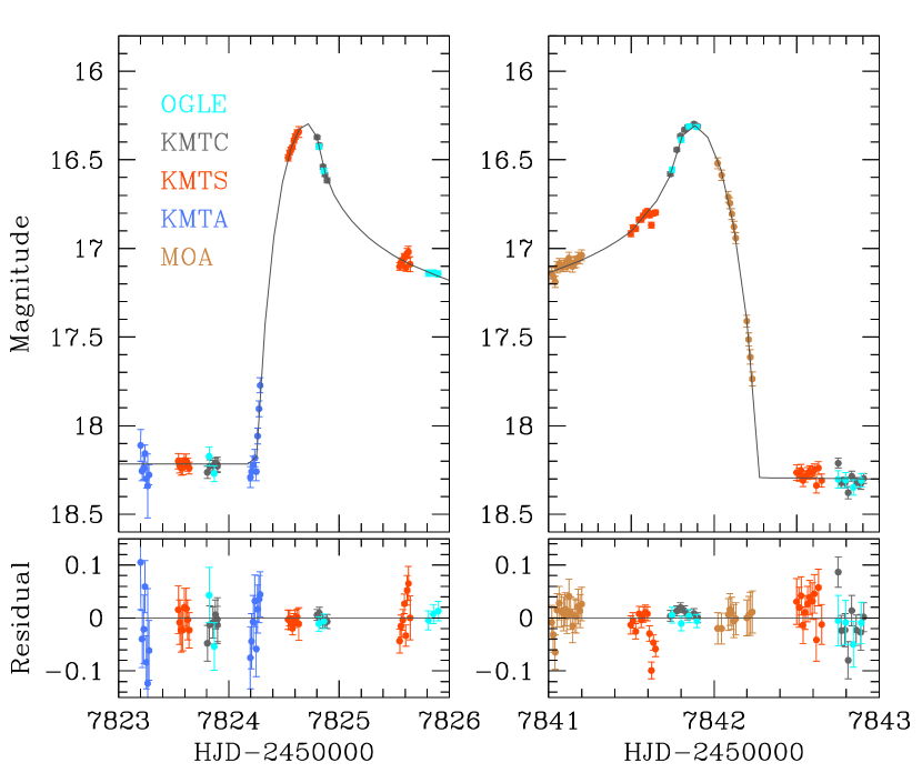
Figure 2.— Zoom of lensing light curve around the caustic crossing regions. The left and right panels show the light curve when the source entered and exited the caustic, respectively. The bottom panels show the residual from the best-fit model.

Table 1Data used in the analysis

Data set		Coverage (HJD′)	$N_{\rm data}$
OGLE		5376 – 8236	5751
KMTNet	KMTA	7444 – 8220	2237
	KMTC	7439 – 8216	2842
	KMTS	7441 – 8216	3739
MOA		7800 – 7860	268

Two factors make the event scientifically important. The first factor is that the duration of the event is very long. The lensing-induced magnification of the source flux started in the 2016 season and lasted throughout the 2017 season. Due to the long duration of the event, the chance to measure the microlens parallax is high. The second factor is that both of the caustic crossings when the source entered and exited the caustic were densely and continuously covered from the combined observations using the globally distributed telescopes. In Figure 2, we present the zoom of the light curve during the caustic entrance (left panels) and exit (right panels). Analysis of the caustic-crossing parts of the light curve enables one to measure the angular Einstein radius. Being able to measure both $\pi_{\rm E}$ and $\theta_{\rm E}$, then, one can uniquely determine the mass and distance to the lens. This also enables one to check the lens origin of the blended flux.

In Table 1, we list details about the data used in the analysis. The coverage column indicates the time range, and $N_{\rm data}$ represents the number of data points in the individual data sets. For the OGLE data set, we use 9 years of data from 2010 to 2018 for the secure measurement of the baseline magnitude. Although the event was observed by the KMTNet survey since its commencement in 2015, the system was under development during the 2015 season. We, therefore, use KMTNet data that have been acquired since 2016 season after the system was stabilized. For the MOA data, photometric uncertainties of the data near the baseline are considerable, but the data densely covered the caustic exit. We, therefore, use partial MOA data around caustic-crossing features obtained during $7800\lesssim{\rm HJD}^{\prime}\lesssim 7860$.

3. Analysis

Considering the caustic-crossing features, we model the observed light curve based on the binary-lens interpretation. We start modeling under the assumption that the relative lens-source motion is rectilinear although it is expected that the motion would be non-rectilinear due to the long duration of the event. Under this assumption, a lensing light curve is described by 7 principal parameters. Four of these parameters describe the lens-source approach including the time of the closest source approach to a reference position of the lens, $t_{0}$, the source-reference separation at that time, $u_{0}$ (impact parameter), the event time scale, $t_{\rm E}$, and the angle between the source trajectory and the binary axis, $\alpha$ (source trajectory angle). For the reference position of the lens, we use the center of mass of the binary lens system. Another two parameters describe the binary lens including the projected binary separation normalized to $\theta_{\rm E}$, $s$, and the mass ratio between the binary lens components, $q$. The last parameter is the normalized source radius $\rho$, which is defined as the ratio of the angular source radius $\theta_{*}$ to the angular Einstein radius, i.e., $\rho=\theta_{*}/\theta_{\rm E}$.

In the preliminary modeling, we conduct a grid search for the binary-lens parameters $s$ and $q$ while other parameters are searched for using a downhill approach. For the downhill approach, we use the Markov Chain Monte Carlo (MCMC) method. From this preliminary search, we find two candidate solutions with $(s,q)_{\rm close}\sim(0.84,0.13)$ and $(s,q)_{\rm wide}\sim(1.61,0.20)$. We designate the individual solutions as “close” and “wide” based on the fact that the projected binary separation is less ($s<1$) and greater ($s>1$) than the angular Einstein radius, respectively.

Although the solutions found from the preliminary modeling describe the overall light curve, they leave subtle long-term residuals from the models. It is known that long-term deviations are caused by two major higher-order effects. The first one is the microlens-parallax effect that is caused by the orbital motion of Earth (Gould, 1992). The other one is caused by the orbital motion of the lens, lens-orbital effects (Dominik, 1998; Ioka et al., 1999). We, therefore, check whether the fit improves with the consideration of these higher-order effects.

Table 2Comparison of models

Model		$\chi^{2}$
		Close	Wide
Static		16081.8	15634.0
Orbit		15476.8	15565.7
Parallax	($u_{0}>0$)	15886.7	15565.6
–	($u_{0}<0$)	15862.8	15575.4
Orbit+Parallax	($u_{0}>0$)	15355.8	15479.2
–	($u_{0}<0$)	15362.2	15463.4

Consideration of the microlens-parallax effect requires one to include two additional lensing parameters of $\pi_{{\rm E},N}$ and $\pi_{{\rm E},E}$. They represent the north and east components of the microlens-parallax vector, $\mbox{\boldmath$\pi$}_{\rm E}$, projected onto the sky along the north and east equatorial coordinates, respectively. The magnitude of the microlens-parallax vector is $\pi_{\rm E}=(\pi_{{\rm E},N}^{2}+\pi_{{\rm E},E}^{2})^{1/2}$ and it is directed toward the same direction as that of the relative lens-source proper motion vector $\mu$, i.e., $\mbox{\boldmath$\pi$}_{\rm E}=\pi_{\rm E}(\mbox{\boldmath$\mu$}/\mu)$. Consideration of the lens-orbital effect also requires additional parameters. Under the approximation that the change of the lens position is small, the effect is described by two parameters of $ds/dt$ and $d\alpha/dt$, which represent the rates of change in the projected binary separation and the source trajectory angle, respectively.

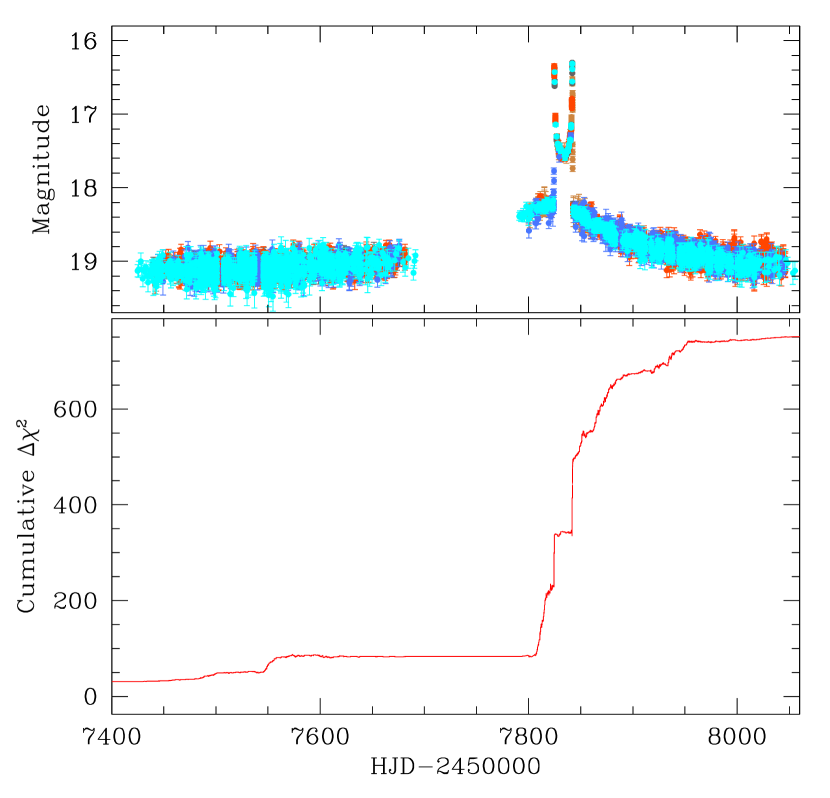
Figure 3.— Cumulative distribution of $\Delta\chi^{2}$ between the models with and without the consideration of the microlens-parallax and lens-orbital effects. The light curve in the upper panel is presented to show the region of fit improvement.

In Table 2, we list the results of the additional modeling considering the higher-order effects. We compare the goodness of the fit for the individual models in terms of $\chi^{2}$ values. The “static” model denotes the solution obtained under the assumption of the rectilinear relative lens-source motion. In the “orbit” and “parallax” models, we separately consider the microlens-parallax and the lens-orbital effects, respectively. In the “orbit+parallax” model, we simultaneously consider both higher-order effects. For microlensing solutions obtained considering microlens-parallax effects, it is known that there may exist a pair of degenerate solutions with $u_{0}>0$ and $u_{0}<0$ due to the mirror symmetry of the source trajectories with respect to the binary axis between the two degenerate solutions: ecliptic degeneracy (Smith et al., 2003; Skowron et al., 2011). We, therefore, check the ecliptic degeneracy whenever parallax effects are considered in modeling. The lensing parameters of the pair of solutions caused by the ecliptic degeneracy are roughly in the relation $(u_{0},\alpha,\pi_{{\rm E},N},d\alpha/dt)\leftrightarrow-(u_{0},\alpha,\pi_{{\rm E},N},d\alpha/dt)$.

From the comparison of $\chi^{2}$ values between the close and wide binary solutions, it is found that the close solution is preferred over the wide solution by $\Delta\chi^{2}\sim 123$. This is statistically significant enough to resolve the degeneracy between the two solutions.

We find that consideration of the higher-order effects significantly improves the fit. It is found that the higher-order effects improve the fit by $\Delta\chi^{2}\sim 726$ for the close-binary solution, which provides the best-fit solution. For the pair of solutions resulting from the ecliptic degeneracy, it is found that the degeneracy is moderately severe with $\Delta\chi^{2}\sim 6.4$, and the $u_{0}>0$ solution is preferred over the $u_{0}<0$ solution. In order to better show the region of fit improvement by the higher-order effects, in Figure 3, we present the cumulative distribution of $\Delta\chi^{2}$, where $\Delta\chi^{2}$ represents the difference in $\chi^{2}$ between the static and orbit+parallax ($u_{0}>0$) models. It shows that the fit improvement occurs throughout the event.

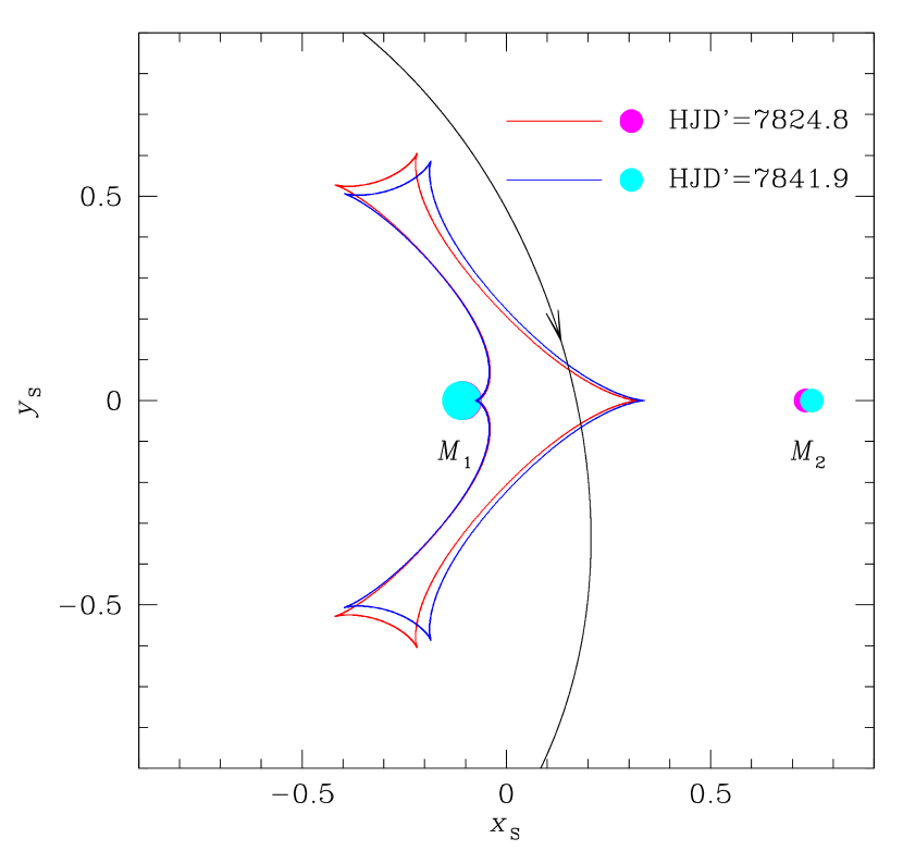
Figure 4.— Configuration of the lens system. The curve with an arrow represents the source trajectory. The closed curve composed of 6 folds represent the caustic. The small filled dots marked by $M_{1}$ and $M_{2}$ represent the positions of the binary-lens components. All lengths are scaled to the angular Einstein radius corresponding to the total mass of the lens. Due to the orbital motion of the lens, the positions of the lens components and the caustic shape vary in time. We mark the positions at HJD^′=7824.8 and 7841.9, which correspond to the times of source star’s caustic entrance and exit, respectively.

In Table 3, we list the lensing parameters determined from modeling. Although the close/wide degeneracy is clearly resolved, we present the parameters of the wide-binary solution for readers who may want to reproduce the result. In Figure 4, we also present the lens-system configuration in which the source trajectory (curve with an arrow) with respect to the binary lens components (marked by $M_{1}$ and $M_{2}$) and the caustic (cuspy closed figure) is shown. According to the best-fit model (close $u_{0}>0$ solution), it is found that the lensing event was produced by a binary with $(s,q)\sim(0.85,0.15)$. Due to the proximity of the binary separation to the angular Einstein radius, the caustics form a single closed curve composed of 6 folds. Due to the relatively low mass ratio, $q\sim 0.15$, the caustic is tilted toward heavier-mass lens component, i.e., $M_{1}$, with a protruding cusp pointing toward the lower-mass lens component, $M_{2}$. The source passed through the protruding cusp region of the caustic, producing the two observed spikes when it entered and exited the caustic. The source trajectory is curved by the higher-order effects, especially by the lens-orbital effect. The change rate of the source trajectory angle is $|d\alpha/dt|\sim 1.22~{}{\rm rad}~{}{\rm yr}^{-1}\sim 70^{\circ}~{}{\rm yr}^{-1}$.

Table 3Lensing parameters

Parameter	Close		Wide
	$u_{0}>0$	$u_{0}<0$	$u_{0}>0$	$u_{0}<0$
$\chi^{2}$	15355.8	15362.2	15479.2	15463.4
$t_{0}$ (HJD′)	7829.104 $\pm$ 0.157	7829.248 $\pm$ 0.050	7834.893 $\pm$ 0.018	7834.209 $\pm$ 0.206
$u_{0}$	0.167 $\pm$ 0.003	-0.161 $\pm$ 0.001	0.026 $\pm$ 0.001	-0.007 $\pm$ 0.006
$t_{\rm E}$ (days)	130.53 $\pm$ 1.00	133.57 $\pm$ 0.53	152.10 $\pm$ 0.178	150.34 $\pm$ 0.44
$s$	0.845 $\pm$ 0.005	0.834 $\pm$ 0.001	1.667 $\pm$ 0.001	1.646 $\pm$ 0.007
$q$	0.147 $\pm$ 0.003	0.149 $\pm$ 0.001	0.232 $\pm$ 0.001	0.223 $\pm$ 0.004
$\alpha$ (rad)	1.344 $\pm$ 0.004	-1.348 $\pm$ 0.004	-1.339 $\pm$ 0.002	1.341 $\pm$ 0.003
$\rho$ ($10^{-3}$)	1.75 $\pm$ 0.01	1.72 $\pm$ 0.01	1.70 $\pm$ 0.01	1.73 $\pm$ 0.01
$\pi_{{\rm E},N}$	-0.049 $\pm$ 0.008	0.050 $\pm$ 0.008	-0.004 $\pm$ 0.003	0.013 $\pm$ 0.007
$\pi_{{\rm E},E}$	0.038 $\pm$ 0.004	0.037 $\pm$ 0.003	0.049 $\pm$ 0.002	0.038 $\pm$ 0.004
$ds/dt$ (yr-1)	0.383 $\pm$ 0.013	0.372 $\pm$ 0.009	0.369 $\pm$ 0.014	0.370 $\pm$ 0.044
$d\alpha/dt$ (rad yr-1)	1.220 $\pm$ 0.021	-1.233 $\pm$ 0.003	-0.026 $\pm$ 0.002	0.006 $\pm$ 0.013

We note that the microlens-parallax parameters are well determined despite their small values. Figure 5 shows the distribution of points in the MCMC chain on the $\pi_{{\rm E},N}$ – $\pi_{{\rm E},E}$ parameter plane. It shows that despite the small magnitude $\pi_{\rm E}=(\pi_{{\rm E},N}^{2}+\pi_{{\rm E},E}^{2})^{1/2}\sim 0.06$, the microlens parallax is precisely measured to be clearly distinguished from a zero-parallax model. This became possible mainly due to the long time scale of the event, which is measured to be $t_{\rm E}\sim 130$ days.

4. Physical Lens Parameters

4.1. Angular Einstein Radius

In addition to the microlens parallax, one needs to measure the angular Einstein radius for the unique determinations of the lens mass and distance. The angular Einstein radius is measured from the normalized source radius by

$$\theta_{\rm E}={\theta_{*}\over\rho}.$$ (3)

The normalized radius is precisely determined from modeling. Then, one needs to measure $\theta_{*}$ to determine $\theta_{\rm E}$.

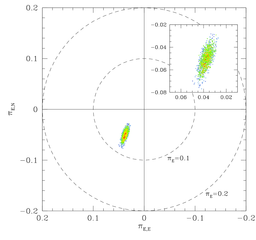
Figure 5.— $\Delta\chi^{2}$ map of MCMC points in the $\pi_{{\rm E},N}$ – $\pi_{{\rm E},E}$ parameter plane for the best-fit solution (“orbit+parallax” solution with $u_{0}>0$). The color coding represents the points of MCMC chain within 1$\sigma$ (red), 2$\sigma$ (yellow), 3$\sigma$ (green), 4$\sigma$ (cyan), and 5$\sigma$ (blue). The inset shows the zoom of the MCMC-point distribution.

We measure the angular source radius from the de-reddened color $(V-I)_{0}$ and magnitude $I_{0}$. In Figure 6, we mark the position of the source in the color-magnitude diagram (CMD) constructed based on the pyDIA photometry of the KMTC data set. To obtain $(V-I)_{0}$ and $I_{0}$, we calibrate the instrumental color and magnitude using the centroid of red giant clump (RGC), for which its de-reddened color and magnitude $(V-I,I)_{0,{\rm RGC}}=(1.06,14.29)$ (Bensby et al., 2011; Nataf et al., 2013) are known, as a reference (Yoo et al., 2004). The locations of the source and RGC centroid in the instrumental CMD are $(V-I,I)_{\rm S}=(1.17,17.25)$ and $(V-I,I)_{\rm RGC}=(1.59,13.76)$, respectively. Then, the de-reddened color and magnitude of the source are estimated from the offsets in color $\Delta(V-I)=(V-I)_{\rm S}-(V-I)_{\rm RGC}$ and magnitude $\Delta I=I_{\rm S}-I_{\rm RGC}$ with respect to the RGC centroid by $(V-I,I)_{0,{\rm S}}=[(V-I)_{0,{\rm RGC}}+\Delta(V-I),I_{0,{\rm RGC}}+\Delta I]=(0.65\pm 0.02,17.78\pm 0.01)$. The estimated de-reddened color and magnitude indicates that the source is likely to be a metal-poor turnoff star. The measured $V-I$ color is converted into $V-K$ color using the color-color relation of Bessell & Brett (1988) and the angular source radius is estimated using the relation between $V-K$ and the surface brightness of Kervella et al. (2004). The measured angular source radius is $\theta_{*}=1.04\pm 0.08~{}\mu$as.

In Table 4, we list the measured angular Einstein radius. We also present the relative lens-source proper motions in the geocentric, $\mu_{\rm geo}$, and heliocentric frames, $\mu_{\rm helio}$. The geocentric proper motion vector is determined from the measured angular Einstein radius, event time scale, and microlens parallax vector $\mbox{\boldmath$\pi$}_{\rm E}=(\pi_{{\rm E},N},\pi_{{\rm E},E})$ by

$$\mbox{\boldmath$\mu$}_{\rm geo}={\theta_{\rm E}\over t_{\rm E}}{\mbox{\boldmath$\pi$}_{\rm E}\over\pi_{\rm E}}.$$ (4)

The heliocentric proper motion is computed by

$$\mbox{\boldmath$\mu$}_{\rm helio}=\mbox{\boldmath$\mu$}_{\rm geo}+{\bf v}_{\oplus,\perp}{\pi_{\rm rel}\over{\rm au}},$$ (5)

where ${\bf v}_{\oplus,\perp}$ represents the velocity of the Earth motion projected on the sky at $t_{0}$ and $\pi_{\rm rel}=\pi_{\rm L}-\pi_{\rm S}={\rm au}(D_{\rm L}^{-1}-D_{\rm S}^{-1})$ is the relative lens-source parallax (Gould, 2004; Dong et al., 2009). The angle $\phi$ represents the orientation angle of $\mbox{\boldmath$\mu$}_{\rm helio}$ as measured from the north. It is found that the measured Einstein radius $\theta_{\rm E}\sim 0.6$ mas is close to that of a typical lensing event. However, the measured relative lens-source proper motion, $\mu_{\rm geo}\sim 1.7~{}{\rm mas}~{}{\rm yr}^{-1}$, is substantially slower than a typical value of $\sim 5~{}{\rm mas}~{}{\rm yr}^{-1}$. This indicates that the long time scale of the event is mainly caused by the slow relative lens-source motion. From simulation of Galactic lensing events, Han et al. (2018) pointed out that majority of long time-scale events are caused by slow relative lens-source proper motions arising due to the chance alignment of the lens and source motions. In this sense, OGLE-2017-BLG-0039 is a typical long time-scale event.

Figure 6.— Location of the source and blend with respect to the centroid of the red giant clump (RGC) in the instrumental color-magnitude diagram. Also marked is the position of the lens expected from the determined mass and distance.

4.2. Mass and Distance

We estimate the mass and distance to the lens using Equations (1) and (2) and list them in Table 5. Also listed are the projected separation $a_{\perp}=sD_{\rm L}\theta_{\rm E}$ and the projected kinetic-to-potential energy ratio $({\rm KE}/{\rm PE})_{\perp}$. The projected kinetic-to-potential energy ratio is computed based on the projected binary separation $a_{\perp}$, lens mass $M=M_{1}+M_{2}$, and the lensing parameters $s$, $ds/dt$, and $d\alpha/dt$ by

$$\left({{\rm KE}\over{\rm PE}}\right)_{\perp}={(a_{\perp}/{\rm au})^{3}\over 8\pi^{2}(M/M_{\odot})}\left[\left({1\over s}{ds/dt\over{\rm yr}^{-1}}\right)^{2}+\left({d\alpha/dt\over{\rm yr}^{-1}}\right)^{2}\right].$$ (6)

The ratio should be less than unity for the lens system to be a gravitationally bound system. It is found that the measured ratios for both the $u_{0}>0$ and $u_{0}<0$ solutions satisfy this condition. Furthermore, the estimated kinetic-to-potential energy ratio is within the expected range $0.2\lesssim({\rm KE/PE})_{\perp}\lesssim 0.5$ for binaries with moderate orbital eccentricity that are not viewed at unusual angles, e.g., a wide binary in an edge-on orbit.

Table 4Angular Einstein radius and the relative lens-source proper motion

Parameter	Value
$\theta_{\rm E}$ (mas)	0.59 $\pm$ 0.04
$\mu_{\rm geo}$ (mas yr-1)	1.67 $\pm$ 0.12
$\mu_{\rm helio}$ (mas yr-1)	1.64 $\pm$ 0.12
$\phi$	142∘ (35∘)

According to the best-fit solution, the estimated masses of the primary, $M_{1}\sim 1.0~{}M_{\odot}$, and the companion, $M_{2}\sim 0.15~{}M_{\odot}$, of the lens correspond to the masses of an early G-type and a late M-type dwarfs, respectively. The estimated distance to the lens is $D_{\rm L}\sim 6.0$ kpc.

4.3. Flux from the Lens

The estimated mass of the primary lens, $M_{1}\sim 1.0~{}M_{\odot}$, is substantially heavier than those of the most common lens population of M dwarfs. If the lens is a star, then, its flux will contribute to the blended flux.

In Figure 6, we mark the position of the primary lens, which dominates the flux from the binary lens, in the instrumental CMD expected from the determined lens mass and distance. Here we assume that the primary lens is a main-sequence star and the ranges of the color and magnitude are estimated based on the uncertainty of the estimated lens mass. Because the estimated distance to the lens, $D_{\rm L}\sim 6$ kpc, indicates that the lens is likely to be located behind most obscuring dust in the disk, the lens experiences extinction and reddening similar to those of the source star. Under this assumption, we estimate the lens position in the CMD by

$$(V-I,I)_{\rm L}=(V-I,I)_{0,{\rm L}}+[(V-I,I)_{\rm RGC}-(V-I,I)_{0,{\rm RGC}}],$$ (7)

where $(V-I,I)_{\rm RGC}=(1.59,13.76)$ represent the apparent color and magnitude of the RGC centroid in the instrumental CMD and $(V-I,I)_{0,{\rm RGC}}=(1.06,14.29)$ represent the de-reddened values. The color $(V-I)_{0,{\rm L}}\sim 0.68$ represents the intrinsic color corresponding to the estimated lens mass (Allen, 1976). The de-reddened lens magnitude is estimated by

$$I_{0,{\rm L}}=[M_{V}-(V-I)_{0,{\rm L}}]+5\ \log(D_{\rm L}/{\rm pc})-5,$$ (8)

where $M_{V}\sim 4.7$ is the absolute $V$-band magnitude of a main-sequence star with a mass corresponding to the lens mass (Allen, 1976). The estimated color and magnitude of the lens in the instrumental CMD are $(V-I,I)_{\rm L}=(1.21_{-0.06}^{+0.07},17.37_{-0.73}^{+0.54})$. Also marked in the CMD is the location of the blend (square dot) which has color and brightness of $(V-I,I)_{b}=(1.44,16.93)$. It is found that the position of the lens in the CMD is close to that of the blend.

Table 5Physical lens parameters.

Parameter	$u_{0}>0$	$u_{0}<0$
$M_{1}$ ($M_{\odot}$)	1.03 $\pm$ 0.15	1.03 $\pm$ 0.15
$M_{2}$ ($M_{\odot}$)	0.15 $\pm$ 0.02	0.15 $\pm$ 0.02
$D_{\rm L}$ (kpc)	5.99 $\pm$ 0.77	5.94 $\pm$ 0.76
$a_{\perp}$ (au)	3.00 $\pm$ 0.39	2.99 $\pm$ 0.38
$({\rm KE}/{\rm PE})_{\perp}$	0.49 $\pm$ 0.02	0.49 $\pm$ 0.02

The proximity of the lens position to that of the blend in the CMD indicates that the flux from the lens comprises a significant fraction of the blended flux. From the comparison of the $I$-band magnitudes of the lens and blend, it is found that the lens is $\Delta I\sim 0.44$ magnitude fainter than the total blended flux. Because the flux from the lens contributes to the blended flux, this means that the lens comprises $\sim 2/3$ of the $I$-band blended flux, although this fraction is somewhat uncertain due to the uncertainty of the lens brightness. The lens is bluer than the blend by $\Delta(V-I)\sim 0.23$. This indicates the possibility that there may exist another blended star that is redder than the lens. An alternative explanation of the slight differences in color and brightness between the lens and blend is that the lens is a “turnoff star” rather than a main-sequence star. Since a turnoff star has evolved off the main sequence, it is slightly redder and brighter than a main sequence star with a same mass.

In order to check the two possible explanations for the slight differences in the color and brightness between the lens and blend, we measure the “astrometric offset” between the source and baseline object using the OGLE images. If there exists another blend, the position of the baseline object, which corresponds to the centroid of the combined image of the blend and source, would be slightly different from the position when the source is magnified, and thus there would be an astrometric offset. If the “turnoff star” explanation is correct, on the other hand, there would be no measurable astrometric offset. From this measurement, we find that the image centroid when the source was magnified is shifted from the baseline object by $\sim 0.26\pm 0.07$ pixels, which corresponds to $\sim 65\pm 17$ mas. This supports the explanation that there is another blend.

5. Conclusion

We analyzed the binary-lensing event OGLE-2017-BLG-0039. The long duration of the event enabled us to precisely measure the microlens parallax despite the small value. In addition, the analysis of the well resolved caustic crossings during both source star’s entrance and exit of the caustic allowed us to measure the angular Einstein radius. From the combination of $\pi_{\rm E}$ and $\theta_{\rm E}$, we measured the mass and distance to the lens and found that the lens was a binary composed of an early G and late M dwarfs located at a distance $\sim 6$ kpc. From the location of the lens in the color-magnitude diagram, it was found that the flux from the lens comprised $\sim 2/3$ of the blended light. Therefore, the event was a rare case of a bright lens event for which follow-up spectroscopic observations could confirm the nature of the lens.

References

- Albrow (2017) Albrow, M. 2017, MichaelDAlbrow/pyDIA: Initial Release on Github, doi:10.5281/zenodo.268049
- Alcock et al. (2001) Alcock, C., Allsman, R. A., Alves, D. R., et al. 2001, Nature, 414, 617
- Allen (1976) Allen, C. W. 1976, Allen’s Astrophysical Quantities, Fourth Edition, eds. A. N. Cox (Springer: New York)
- Batista et al. (2015) Batista, V., Beaulieu, J.-P., Bennett, D. P., et al. 2015, ApJ, 808, 170
- Beaulieu et al. (2016) Beaulieu, J.-P., Bennett, D. P., Batista, V., et al. 2016, ApJ, 824, 83
- Bessell & Brett (1988) Bessell, M. S., & Brett, J. M. 1988, PASP, 100, 1134
- Boden et al. (1998) Boden, A. F., Shao, M., & Van Buren, D. 1998, ApJ, 502, 538
- Bond et al. (2004) Bond, I. A., Udalski, A., Jaroszyński, M., et al. 2004, ApJ, 606, L155
- Bennett et al. (2006) Bennett, D. P., Anderson, J., Bond, I. A., Udalski, A., & Gould, A. 2006, ApJ, 647, L171
- Bennett et al. (2007) Bennett, D. P., Anderson, J., & Gaudi, B. S. 2007, ApJ, 660, 781
- Bennett et al. (2015) Bennett, D. P., Bhattacharya, A., Anderson, J., et al. 2015, ApJ, 808, 169
- Bennett et al. (2010) Bennett, D. P., Rhie, S. H., Nikolaev, S., et al. 2010, ApJ, 713, 837
- Bensby et al. (2011) Bensby, T., Adén, D., Meéndez, J., et al. 2011, PASP, 533, 13
- Bond et al. (2001) Bond, I. A., Abe, F., Dodd, R. J., et al. 2001, MNRAS, 327, 868
- Choi et al. (2012) Choi, J.-Y., Shin, I.-G., Park, S.-Y., et al. 2012, ApJ, A751, 41
- Chung et al. (2017) Chung, S.-J., Zhu, W., Udalski, A., et al. 2017, ApJ, 838, 154
- Dominik (1998) Dominik, M. 1998, A&A, 329, 36
- Dong et al. (2009) Dong, S., Gould, A., Udalski, A., et al. 2009, ApJ, 695, 970
- Gaudi et al. (2008) Gaudi, B. S., Bennett, D. P., Udalski, A., et al. 2008, Science, 319,
- Gould (1992) Gould, A. 1992, ApJ, 392, 442
- Gould (1994) Gould, A. 1994, ApJ, 421, L75
- Gould (1997) Gould, A. 1997, ApJ, 480, 188
- Gould (2000) Gould, A. 2000, ApJ, 542, 785
- Gould (2004) Gould, A. 2004, ApJ, 606, 31
- Gould et al. (2009) Gould, A., Udalski, A., Monard, B., et al. 2009, ApJ, 698, L147
- Han & Chang (2003) Han, C., & Chang, H.-Y. 2003, MNRAS, 338, 637
- Han & Gould (2003) Han, C., & Gould, A. 2003, ApJ, 592, 172
- Han & Jeong (1999) Han, C., & Jeong, Y. 1999, MNRAS, 309, 404
- Han et al. (2018) Han, C., Jung, Y. K., Shvartzvald, Y., et al. 2018, ApJ, in press
- Han et al. (2013) Han, C., Udalski, A., Choi, J.-Y., et al. 2013, ApJ, 762, L28
- Høg et al. (1995) Høg, E., Novikov, I. D., & Polnarev, A. G. 1995, A&A, 294, 287
- Ioka et al. (1999) Ioka, K., Nishi, R., & Kan-Ya, Y. 1999, PThPh, 102, 98
- Jeong et al. (1999) Jeong, Y., Han, C., Park, & S.-H. 1999, ApJ, 511, 569
- Kervella et al. (2004) Kervella, P., Thévenin, F., Di Folco, E., & Ségransan, D. 2004, A&A, 426, 29
- Kozłowski et al. (2007) Kozłowski, S., Woźniak, P. R., Mao, S., & Wood, A. 2007, ApJ, 671, 420
- Kim et al. (2016) Kim, S.-L., Lee, C.-U., Park, B.-G., et al. 2016, JKAS, 49, 37
- Miyamoto & Yoshii (1995) Miyamoto, M., & Yoshii, Y. 1995, AJ, 110, 1427
- Nataf et al. (2013) Nataf, D. M., Gould, A., Fouqué, P., et al. 2013, ApJ, 769, 88
- Paczyński (1998) Paczyński B. 1998, ApJ, 494, L23
- Refsdal (1966) Refsdal, S. 1966, MNRAS, 134, 315
- Sahu et al. (2017) Sahu, K. C., Anderson, J., Casertano, S., et al. 2017, Science, 356, 1046
- Shin et al. (2018) Shin, I.-G., Udalski, A., Yee, J. C., et al. 2018, AAS, submitted, arxiv:1801.00169
- Shvartzvald et al. (2018) Shvartzvald, Y., Yee, J. C., Skowron, J., et al. 2018, AAS, submitted, arxiv:1805.08778
- Skowron et al. (2011) Skowron, J., Udalski, A., Gould, A., et al. 2011, ApJ, 738, 87
- Smith et al. (2003) Smith, M. C., Mao, S., & Paczyński, B. 2003, MNRAS, 339, 925
- Udalski et al. (2005) Udalski, A., Jaroszyński, M., Paczyński, B., et al. 2005, ApJ, 628, L109
- Udalski et al. (2015) Udalski, A., Szymański, M. K., & Szymański, G. 2015, AcA, 65, 1
- Udalski (2003) Udalski, A. 2003, AcA, 53, 291
- Walker (1995) Walker M. A. 1995, ApJ, 453, 37
- Yee et al. (2009) Yee, J. C., Udalski, A., Sumi, T., et al. 2009, ApJ, 703, 2082
- Yoo et al. (2004) Yoo, J., DePoy, D. L., Gal-Yam, A., et al. 2004, ApJ, 603, 139
- Zang et al. (2018) Zang, W., et al., 2018, in preparation
- Zhu et al. (2016) Zhu, W., Calchi Novati, S., Gould, A., et al. 2016, ApJ, 825, 60
- Zurlo et al. (2018) Zurlo, A., Gratton, R., Mesa, D., et al. 2018, MNRAS, 480, 236