Constraining small scale magnetic fields through plasma lensing: Application to the Black widow eclipsing pulsar binary

Abstract

In regions with strongly varying electron density, radio emission can be magnified significantly by plasma lensing. In the presence of magnetic fields, magnification in time and frequency will be different for two circular polarizations. We show how these effects can be used to measure or constrain the magnetic field parallel to the line of sight, $B_{\parallel}$, as well as its spatial structure, $\sigma_{B_{\parallel}}$, in the lensing region. In addition, we discuss how generalized Faraday rotation can constrain the strength of the perpendicular field, $B_{\perp}$. We attempt to make such measurements for the Black Widow pulsar, PSR B1957+20, in which plasma lensing was recently discovered. For this system, pressure equilibrium suggests $B\gtrsim 20\,$G at the interface between the pulsar and companion winds, where the radio eclipse starts and ends, and where most lensing occurs. We find no evidence for large-scale magnetic fields, with, on average, $B_{\parallel}=0.02\pm 0.09\,$G over the egress lensing region. From individual lensing events, we strongly constrain small scale magnetic structure to $\sigma_{B}<10\,$mG, thus excluding scenarios with a strong but rapidly varying field. Finally, from the lack of reduction of average circular polarization in the same region, we rule out a strong, quasi-transverse field. We cannot identify any plausible scenario in which a large magnetic field in this system is concealed, leaving the nature of the interface between the pulsar and companion winds an enigma. Our method can be applied to other sources showing plasma lensing, including other eclipsing pulsars and fast radio bursts, to study the local properties of the magnetic field.

1 Introduction

The success of gravitational lensing shows that a remarkable amount of information about the material distribution along the line of sight can be gleaned from the bending and delaying of light (eg. Schneider et al. 1992). At radio frequencies, lensing by plasma can similarly illuminate structures in the interstellar medium (see, e.g., Tuntsov et al. 2016). Unlike gravitational lenses, plasma lenses are highly chromatic, as the refractive index of a plasma depends on the frequency of light. Moreover, in the presence of magnetic fields, the refractive indices of the left and right circular polarization states differs, a phenomenon known as birefringence. Birefringence is sensitive to spatial structure of the magnetic fields, and completely predictable in the case of a uniform magnetic field. It thus serves as a probe for magnetic properties at the location of lenses.

For conditions typical of the interstellar medium, with magnetic field strengths of order tens of $\mu$G, the effects are relatively small, but stronger fields are encountered in supernova remnants and in binary systems in which the companion is loosing mass. Of particular interest here are the so-called “Black Widow” and “Redback” pulsar binaries, in which the pulsar signal is seen to be dispersed or removed by plasma associated with the companion. This plasma also can lens the pulsar, as recently found for the original Black Widow binary, PSR B1957+20, where in regions near the radio eclipse the pulses not only show variations in dispersive delay of order 1 $\mu$s on a timescale of 2 s, but also in amplitude, with magnifications reaching nearly two orders of magnitude (Main et al., 2018). The variable magnifications are best explained through plasma lensing, and here we show how the flux modulation versus time, frequency and polarization from the brightest events helps constrain the magnetic properties of these plasma lenses.

The paper is organized as follows. In Section 2, we first discuss the properties of PSR B1957+20 and its eclipse, in particular the need of a strong magnetic field to understand the long radio eclipse, and the tension between this expected strong field with previous observational upper limits to the field strength. Next, in Section 3, we illustrate the observable effects of magnetic fields, introducing quantitive methods to use birefringence of plasma lenses, and reviewing methods beyond Faraday rotation. We apply these methods in Section 4, separating what we can learn from normal, lensed, and giant pulses. We infer substantially more stringent upper limits on the magnetic field strength, and discuss their impact on our understanding of the system in Section 5. Finally, in Section 6, we present the ramifications of our results.

2 Motivation for measuring the magnetic field

PSR B1957+20 was the first millisecond pulsar binary found in which the pulsar signal is eclipsed near superior conjunction of its companion (Fruchter et al., 1988). Thirty years after its discovery, many puzzles remain. Most relevant for our purposes are two associated with the eclipse. First, the excess electrons observed near eclipses implies material extending to a distance of $r_{\mathrm{if}}\simeq 0.8\,\hbox{$R_{\odot}$}$ from the companion in the direction perpendicular to the pulsar wind, which is well outside the companion’s Roche lobe; what supports this material against the strong Poynting flux from the pulsar? Second, observations at higher frequency show that when the radio flux is greatly reduced at 318 MHz, the excess electron column density is of order $\sim 0.01\,$${\rm pc/cm}^{3}$(Ryba & Taylor, 1991). For a typical length scale of the system of $\sim\!0.5\,\hbox{$R_{\odot}$}$, this indicates an electron density of only $n_{e}\sim 10^{6}{\rm\,cm^{-3}}$, much lower than required for simple absorption mechanisms like free-free absorption; what then is the mechanism causing the long radio eclipse?

Thompson et al. (1994) suggested a simple solution to both puzzles, viz., that the companion had a magnetic field which was strong enough to lead to a field of 20–40 G at the interface between the companion’s outflow and the pulsar wind. If so, the magnetic pressure would suffice to balance the Pointing flux, thus explaining the long stand-off distance, and synchrotron-cyclotron absorption would suffice to explain the radio eclipse. Measurements by Fruchter et al. (1990), however, constrained the average $\overline{B}_{\parallel}$ to be $<\!6\,$G and $<\!1.5\,$G right before and after the radio eclipse, respectively. Given the discrepancy between these limits and the expected large magnetic fields, it seems well worthwile to attempt to measure the magnetic field more carefully.

2.1 The predicted magnetic strength

If the pulsar wind is balanced by the magnetic pressure of the companion wind at the interface, then

$$P_{\mathrm{pw}}=P_{\mathrm{cw}}=\frac{B_{\mathrm{cw}}^{2}}{8\pi}.$$ (1)

where ‘pw’ indicates pulsar wind, ‘cw’ indicates companion wind.

The pressure of the pulsar wind can be estimated from the spin down energy of the pulsar scaled to the distance of companion:

$$P_{\mathrm{pw}}=\frac{I_{\mathrm{psr}}\Omega\dot{\Omega}}{4\pi a^{2}c},$$ (2)

where $I_{\mathrm{psr}}$ is the pulsar’s moment of inertia, $\Omega\equiv 2\pi/P$ the angular spin frequency, $P$ the spin period, and $a$ the orbital separation. Inserting $a=2.7$ $R_{\odot}$, $P=1.6$ ms, and $\dot{P}=1.7\times 10^{-17}$ ms (Arzoumanian et al., 1994), one infers that to withstand the pulsar wind ram pressure requires a magnetic field strength,

$$B_{\rm cw}=19\,G\,I_{45}^{1/2}\gtrsim 20\,G,$$ (3)

where the moment of inertia is scaled to $10^{45}{\rm\,g\,cm^{2}}$, and the approximate lower limit includes that, for PSR B1957+20, $I_{45}>1.5$ (Steiner et al., 2015) given the lower limit 1.65 $M_{\odot}$ to its mass (van Kerkwijk et al., 2011), and that the above estimate assumes a spherically symmetric pulsar wind, while in reality it is probably focused towards the equatorial plane (in which the companion likely resides).

Given the predicted value of $B_{\mathrm{cw}}\gtrsim 20\,$G at the interface, a simple dipole model yields a surface magnetic field of $B_{\mathrm{comp}}\simeq B_{\mathrm{cw}}(r_{\mathrm{if}}/R_{\mathrm{comp}})^{3}\gtrsim 650$ G (where $R_{\mathrm{comp}}\simeq 0.25\,\hbox{$R_{\odot}$}$; van Kerkwijk et al. 2011). This is quite plausible, given that the companion is a rapidly rotating brown dwarf, and brown dwarfs with surface magnetic fields as high as 5 kG are known (Berdyugina et al., 2017).

2.2 Scenarios for hiding strong fields

Given the arguments above, there should be a strong, $\sim\!20\,$G field that provides pressure balance at the interface, yet such a strong field seems excluded by observational limits. Could it be that the observations are not sensitive to the true field strength?

One possibility arises from the measurement technique: because of the small linear polarization, the best constraints on $\overline{B}_{\parallel}$ from Fruchter et al. (1990) were from measurements of the Faraday group delay between left and right circular polarizations in profiles that were integrated over 10–60 s. As argued by Thompson et al. (1994), however, the magnetic field in the pulsar wind – i.e., well outside the light cylinder where the field cannot corotate – should change direction on a length scale of $cP/2\approx 240$ km. As the Poynting flux hits the magnetized companion wind, rapid reconnection is expected at the interface, and the magnetic field in the companion wind is thus expected to vary on the same length scale. If so, for an observation of Faraday delay made through the reconnection layer, the Faraday delay will be averaged down along the line of sight, and a further reduction will happen by integrating over multiple pulses. To avoid this, one would ideally use single-pulse measurements of the magnetic field, and also obtain constraints on the magnetic variance. We will show in Section 3.1 how birefringence in pulses magnified by plasma lenses can provide such constraints.

Another simple scenario to square the low $B_{\parallel}$ observed with the high expected value is to assume the 20 G magnetic field is nearly perpendicular to the line of sight. As discussed in Section 3.3, this ad hoc assumption can, for sufficiently strong magnetic fields, be tested with generalized Faraday rotation.

Finally, underlying the constraints on the magnetic field is an assumption that it is companion material that is being traversed, i.e., that the excess DM represents excess electrons accompanied by ions. Could it be that the excess material instead consists of electron-positron pairs, either material captured from the pulsar wind (perhaps similar to the solar wind captured in Earth’s Van Allen belts), or pairs created by interaction of the pulsar wind with companion material? In a scenario were the excess DM is due to pairs, no differences in Faraday delay would be expected, since electrons and positrons have opposite and equal effect. An advantage of this more extreme scenario is that it might also help understand the eclipses seen for PSR J1816+4510 (Stovall et al., 2014), whose companion is a proto–white dwarf (Kaplan et al., 2013) for which, unlike for the low-mass companions typically found for eclipsing binary pulsars, no mass loss is expected. As we show below, this scenario can also be tested using generalized Faraday rotation.

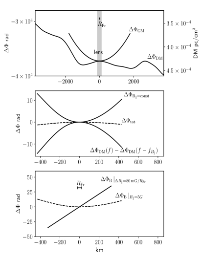
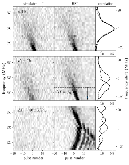
Figure 1: Induced birefringence in plasma lenses due to the influence of magnetic fields on the incoming wavefronts for left and right circular polarizations. The left panels show wavefront phases for left circular polarization (for right polarization, $\Delta\Phi_{B}$ has the opposite sign), while the right panels show sample simulated spectra with cross polarization frequency correlation of pulse number 0 at the side. (Top): Extreme lensing events happen whenever the phase delays $\Delta\Phi_{\mathrm{DM}}$ caused by excess DM happen to cancel out the geometric delays $\Delta\Phi_{\mathrm{GM}}$ over regions larger than the Fresnel scale (for this example, $R_{\rm Fr}=45\,$km) Given the chromaticity of the dispersive delays, the expected spectra are chromatic, and, in the absence of magnetic fields, identical for both polarizations within the noise. (Middle): In the presence of a uniform magnetic field in the plasma lens, convergence in the two polarization states will happen at a different frequency, because the phase gradient induced by a uniform magnetic field can be compensated by a shift in frequency. As a result, the spectra of the two polarizations will be offset by the cyclotron frequency $f_{B_{\parallel}}$. (Bottom): In the presence of magnetic variations in the transverse plane, the coherency of the lens can be destroyed. For a DM of $\sim\!10^{-4}$pc/cm³, a magnetic wedge of $\Delta B_{\parallel}=80\,\mathrm{mG}/R_{\mathrm{Fr}}$ will completely change the curvature of the wavefront, and hence, the two polarizations will not be magnified at the same time. (Note that in the simulation for this case, the ringing results from interference between multiple images at frequencies right below a caustic. This itself is not a magnetic effect, but a modulation that is shifted into the band – it is present below the parts shown also in the other examples.)

3 Observable effects

Evidence for a magnetic field is generally sought via Faraday rotation, but this works only if a source has some linearly polarized emission. Below, we show that plasma lensing can provide strong constraints also for unpolarized sources. Furthermore, we review the constraints possible from regular emission using Faraday delay and generalized Faraday rotation.

3.1 Birefringence in a plasma lens

For a magnetic field of 20 G, one expects significant birefringence in plasma lensing, as well as induced circular polarization on unpolarized sources. Below, we show that birefringence can be identified by looking at the spectra of lensed events in left and right circular flux separately. For a uniform magnetic field, we find that spectra should have frequency offsets, while for a varying magnetic field, we find that the two polarizations should have different magnifications. We illustrate both effects in Figure 1.

3.1.1 Lensing in a magnetoactive cold plasma

When the cyclotron frequency is well below the observation frequency, the natural mode of the plasma will be circularly polarized, leading to different refractive indices for the two circular polarizations,

$$n_{L,R}=\sqrt{1-\frac{f_{p}^{2}}{f(f\mp f_{B_{\parallel}})}}\simeq 1-\frac{1}{2}\,\frac{f_{p}^{2}}{f^{2}}\left(1\pm\frac{f_{B_{\parallel}}}{f}\right)$$ (4)

where $L$, $R$ indicate the two circular polarizations, $f_{p}=\sqrt{n_{e}e^{2}/m_{e}}=1.6\,\mathrm{kHz/cm^{3/2}}\,n_{e}^{1/2}$ is the plasma frequency, $f$ is the observation frequency, $f_{B_{\parallel}}=qB\cos\alpha/2\pi m_{e}=2.8\,\mathrm{MHz/G}\,B_{\parallel}$ is the cyclotron frequency of the parallel magnetic field (with $\alpha$ is the angle between $\vec{B}$ and the line of sight), and the approximate equality holds if $f_{B_{\parallel}}\ll f$ and $f_{p}\ll f$.

For PSR B1957+20, as is often the case, the plasma and cyclotron frequencies are much smaller than the observing frequency: the typical excess DM is of order $10^{-4}\,\hbox{${\rm pc/cm}^{3}$}$, which, combined with a size of order $r_{\mathrm{if}}\simeq 0.4\,\hbox{$R_{\odot}$}$, implies $n_{e}\sim 10^{4}{\rm\,cm^{-3}}$ and thus $f_{p}\sim 1\,$MHz, much smaller than our observing frequency of 330 MHz. Similarly, for a magnetic field strength of $\sim\!20$ G, $f_{B_{\parallel}}\leq f_{B}\sim 60$ MHz, which again is well below 330 MHz.

For this situation, it is useful to define non-magnetic and magnetic breaking index differences $\Delta n_{p}$ and $\Delta n_{B}$, such that $n=1-\Delta n_{p}\mp\Delta n_{B}$. With these, after passing through the plasma, the phase of the electromagnetic wave observed on Earth can be written as a simple integral along the line of sight,

$$\Phi(\vec{x}) =\frac{2\pi}{\lambda}\int(1-\Delta n_{p}\mp\Delta n_{B})dl$$ (5)

$$=\Phi_{\mathrm{GM}}(\vec{x})+\Phi_{\mathrm{DM}}(\vec{x})\pm\Phi_{B}(\vec{x})$$ (6)

where $\vec{x}=(x,y)$ represents position on the lens plane, $\Phi_{\mathrm{GM}}$ the geometric contribution to the phase, $\Phi_{\mathrm{DM}}$ the dispersive contribution, and $\Phi_{B}$ the magnetic contribution.

A pulse will be magnified when the wavefront from a coherent region is flat, ie. if the extra phase from DM and the magnetic field cancels the geometric phase, i.e., when $\Delta\Phi_{\mathrm{GM}}+\Delta\Phi_{\mathrm{DM}}\pm\Delta\Phi_{B}\simeq 0$, with the three phase differences given by,

$$\Delta\Phi_{\mathrm{GM}} =\pi\left(\frac{|\vec{x}|}{R_{\mathrm{Fr}}}\right)^{2}\,$$ (7)

$$\Delta\Phi_{\mathrm{DM}} =2\pi k_{\mathrm{DM}}\Delta\mathrm{DM}(\vec{x})/f\,$$ (8)

$$\Delta\Phi_{B} =\Delta\mathrm{RM}(\vec{x})\lambda^{2}$$ (9)

where $R_{\mathrm{Fr}}=\sqrt{\lambda a}$ is the Fresnel scale, with $a$ the distance between pulsar and the plasma lens and $\lambda\equiv c/f$ the observing wavelength, $\mathrm{D\!M}=\int n_{e}\,dl$ the dispersion measure, $k_{\mathrm{DM}}=e^{2}/2\pi m_{e}c=4149{\rm\,s\,MHz^{2}\,cm^{3}/pc}$ the dispersion constant, and $\mathrm{R\!M}=e^{3}/2\pi m_{e}^{2}c^{4}\,\int n_{e}\Delta B_{\parallel}\,dl$ the rotation measure. (Note that, in contrast to Main et al. (2018), our phases are in radians, not cycles.)

In the above, in principle magnetic fields anywhere along the line of sight could influence the results. The strong lensing events we study, however, last only tens of miliseconds, while scintillation from the interstellar medium (ISM) changes on timescales of minutes (Main et al., 2017). Hence, in our measurements of the magnetic field in the following sections, we can consider the contribution from the interstellar medium constant, and we probe effects due to the magnetic field at the pulsar-companion interface.

3.1.2 Uniform magnetic field

In the presence of a uniform magnetic field, $\Delta\Phi_{B}=\Delta\Phi_{\mathrm{DM}}f_{B_{\parallel}}/f\propto\Delta\mathrm{DM}\,\mathrm{B}_{\parallel}$, and both the variations of $\Delta\Phi_{B}$ and $\Delta\Phi_{\mathrm{DM}}$ are completely determined by the shape of $\Delta\mathrm{DM}$. Therefore, for lensing, the DM has to vary on the same length scale as $\Phi_{\mathrm{GM}}$, i.e., the Fresnel scale, causing opposite phase delays. Furthermore, in order to avoid cancellation, no variations should be present on smaller spatial scales.

The parameter governing birefringence is $B_{\parallel}$. For a uniform magnetic field, the cyclotron frequency $f_{B_{\parallel}}$ will be constant, and the birefringence will be equivalent to a frequency shift. This can be seen by considering the refractive index as some small offset frequency $\Delta f$. To first order,

$$n_{L,R}(f+\Delta f)=1-\frac{1}{2}\,\frac{f_{p}^{2}}{f^{2}}\left(1\pm\frac{f_{B_{\parallel}}}{f}-\frac{2\Delta f}{f}\right)$$ (10)

Therefore, for the same plasma lens in focus at frequency $f$ without a magnetic field, a non-zero $B_{\parallel}$ will lead to the left circular polarization being focused at $f-f_{B_{\parallel}}/2$ and the right circular polarization being focused at $f+f_{B_{\parallel}}/2$. Thus, the two polarizations will have spectra that are offset in frequency by $f_{B_{\parallel}}$, the cyclotron frequency corresponding to the part of the magnetic field in the lens that is directed along the line of sight.

The frequency offset should be present in all images formed in plasma lenses, but it will be measurable only when the magnification spectra are chromatic across the band. Since the larger the lens, the more chromatic an event should be, the most magnified events should be the best candidates for measuring frequency shifts.

3.1.3 Spatially varying magnetic field

In the presence of a spatially varying magnetic field, the magnetically induced phase change results from variations in both DM and $B$, $\Delta\Phi_{B}\propto\Delta\mathrm{DM}\,B_{\parallel}+\mathrm{DM}\,\Delta B_{\parallel}$. As shown in the previous section, the effect of the first term is a shift in focal frequency between the two polarizations.

The effect of the second term cannot be described as simply, but it is possible to constrain its amplitude observationally. In particular, since the sign of $\Delta\Phi_{B}$ is opposite for the two polarizations, it is not possible for the wavefront of both polarizations to be flat at the same time: if light in one polarization is perfectly lensed by a given region, then the magnification in the other polarization will be modified by $|\langle\exp(i\,2\Delta\Phi_{B})\rangle|$, where the average is taken over the lens. For Gaussian fluctuations in $\Delta\Phi_{B}$, the reduction factor equals $\exp(-2\langle\Delta\Phi_{B}^{2}\rangle)$, which leads to the intuitive result that light in both polarizations cannot be magnified similarly at the same time if $\langle\Delta\Phi_{B}^{2}\rangle^{1/2}\gtrsim 1\,$rad.

The constraint on the variations in magnetic field, $\Delta B_{\parallel}$, will depend on the excess DM of the lensing region. For PSR B1957+20, at the orbital phases where most magnified pulses occur, $\Delta\mathrm{DM}\simeq 10^{-4}$ to $10^{-3}\,\hbox{${\rm pc/cm}^{3}$}$. For $\mathrm{DM}=10^{-4}\,\hbox{${\rm pc/cm}^{3}$}$, the constraint that $\langle\Delta\Phi_{B}^{2}\rangle^{1/2}\lesssim 1\,$rad implies $\langle\Delta\hbox{$B_{\parallel}$}^{2}\rangle^{1/2}\lesssim 10\,\mathrm{mG}$, i.e., if there were fluctuations in the magnetic field in excess of $\sim\!10\,$mG on scales of order the Fresnel scale or smaller, one would expect that the magnification would be strongly dependent on circular polarization, and thus that lensing events would be circularly polarized.

3.2 Faraday delay

For a linearly polarized source, magnetized plasma can be easily detected, either from variations in rotation measure or, if the variations are large, from depolarization. In the absence of linearly polarized emission, like for PSR B1957+20, one can measure the magnetic field only when the Faraday rotation is sufficiently large to cause the pulse profiles of the two circular polarizations to be offset in time. This effect is known as Faraday delay (Fruchter et al., 1990), and equals the difference in group delay $\tau_{F}$ between the two circular polarizations,

$$\tau_{F}=\frac{4f_{B_{\parallel}}}{f}\,\tau_{p},$$ (11)

where $\tau_{p}$ is the mean excess dispersive delay of the two polarizations. For $B_{\parallel}=20\,$G and $f=330\,$MHz, one infers $\tau_{F}\simeq 0.7\tau_{p}$. Below, we will compare Faraday delay close to and far away from the eclipse to obtain an independent constraint on $B_{\parallel}$.

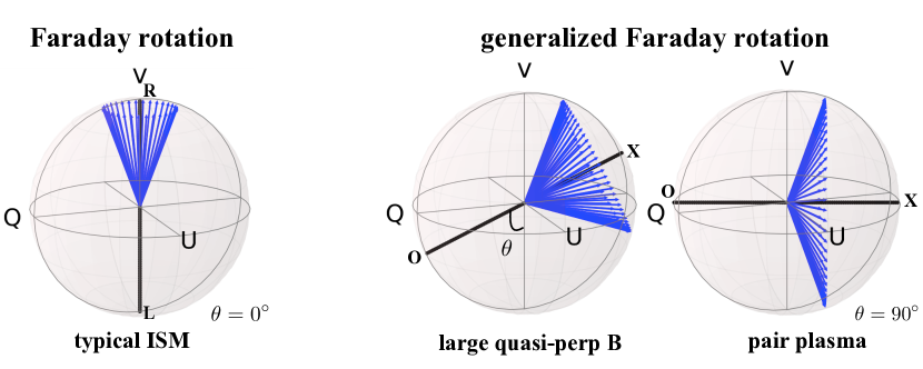
Figure 2: Poincaré spheres showing rotation of the Stokes parameters of an incoming wave (blue arrows) around the natural axis (black bar) of the plasma for three situations, a weak or quasi-parallel magnetic field leading to a natural axis along the polar axis (left), a strong, nearly perpendicular magnetic field giving a large angle $\theta$ from the polar axis (middle), and a purely perpendicular field with an axis in the equatorial plane (right), as appropriate for an electron-positron pair plasma (where the parallel terms cancel). In Faraday rotation (left), the linearly polarized emission is rotated and may become depolarized, but circularly polarized emission is not affected. For the generalized Faraday rotation, linear and circular polarized emission are mixed (and may be depolarized); only the component along the natural axis will remain.

3.3 Generalized Faraday rotation

As noted in Section 2, previous observations found little evidence for parallel magnetic fields in PSR B1957+20, which might imply that the magnetic field is oriented perpendicular to the line of sight, or that the excess dispersion is due to a pair plasma. In either case, there are second-order effects of the magnetic field which, given that the expected cyclotron frequency of $\sim\!60\,$MHz is not that far below our observing frequency of $330\,$MHz, might be detectable.

The effects can be most easily understood by first considering the natural modes of an electromagnetic wave through a magnetized plasma, which propagate independently with different phase velocities. These typically correspond to the two circular polarizations of the wave, and the magnetic field induces Faraday rotation. For a strong magnetic field perpendicular to the line of sight, however, the natural modes are two linear polarizations, ‘o’ and ‘x’, for which the electric vectors are parallel and perpendicular to the magnetic field, respectively, and one expects a rotation between circular and linear polarization.

For the general case, the natural modes are elliptical, and one has generalized Faraday rotation (Kennett & Melrose, 1998). One can visualize the rotation by tracking the change of Stokes parameters against frequency on a Poincaré sphere, as we do in Figure 2. Here, the black axis shows the natural axis of the plasma, which points towards the pole if the natural modes are circular, somewhere along the equator if the natural modes are linear, and at some intermediate angle $\theta$ for the general case. For incoming waves of fixed polarization but different frequencies, passing through a magnetized region will cause the Stokes parameters to be rotated by different amounts, thus leaving them in different directions around the natural axis of the plasma.

The basis of the natural modes can be quantified by a parameter (Thompson et al., 1994),

$$x\equiv 2\left(\frac{f}{f_{B}}\right)\cos\alpha.$$ (12)

where $\alpha$ is the angle between $\vec{B}$ and the line of sight. For typical conditions, with $f_{B}\ll f$ and some random $\alpha$, one has $x\gg 1$, resulting in two circular natural modes. However, $x$ can be small if $\alpha$ is sufficiently close to $90^{\circ}$, and will be zero if the dispersing material consists of a pair plasma.

In terms of $x$, for the general case, the refractive indices for the two natural modes will be, be (Thompson et al., 1994),

$$n^{2}_{\mathrm{1,2}}=1-\frac{f_{p}^{2}}{f^{2}}+\frac{f_{p}^{2}\,f_{B}^{2}}{2f^{4}}\left(1\mp\left(1+x^{2}\right)^{\frac{1}{2}}\right).$$ (13)

Here, for large $x$, one recovers Eq. 4, in which the magnetic term scales linearly with $f_{B}/f$, while for small $x$ it scales quadratically (and is present also for a pair plasma).

For $x\lesssim 1$, the angle $\theta$ between the natural axis of the plasma and the polar axis of the Poincaré sphere is given by,

$$\cot\theta\simeq\frac{4x}{4-x^{2}},$$ (14)

and as $x\to 0$ the phase difference between the two natural modes after passing through the plasma becomes,

$$\Delta\Phi_{\mathrm{x,o}} =\frac{2\pi}{\lambda}\int\left(n_{\mathrm{x}}-n_{\mathrm{o}}\right)\,dl$$ (15)

$$\approx\frac{2\pi}{c}\int\frac{f_{p}^{2}f_{B}^{2}}{2\,f^{3}}\,dl=\Delta\Phi_{\mathrm{DM}}\frac{\langle f_{B_{\perp}}^{2}\rangle}{f^{2}},$$ (16)

where $\langle f_{B_{\perp}}^{2}\rangle$ is an electron-density weighted average.

Note that the phase difference varies as $1/f^{3}$, i.e., faster than the $1/f^{2}$ for Faraday rotation. Without correcting this rotation, the polarized fraction perpendicular to the natural axis will be averaged down almost linearly with the number of turns, leaving only the projection of the initial Stokes parameters onto the natural axis. Inserting numbers for PSR B1957+20, of $\mathrm{DM}=10^{-4}\,\hbox{${\rm pc/cm}^{3}$}$ and $f_{B_{\perp}}=60\,$MHz, and $f=330\,$MHz, one finds $\Delta\Phi_{\mathrm{DM}}\simeq 7900\,$rad, $\Delta\Phi_{\mathrm{x,o}}\simeq 260\,$rad. For a band with a width of 48 MHz centered on 330 MHz, the rotation varies by about 120 rad over the band. Hence, the effect should be significant.

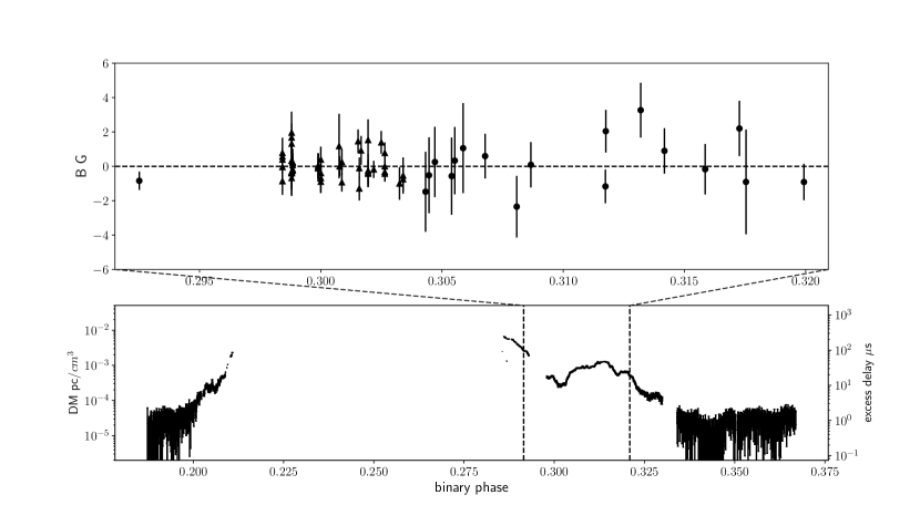
Figure 3: Dispersion and magnetic fields around one eclipse. Bottom: excess dispersion measure inferred from excess delay in arrival times (right axis) of pulse profiles integrated in 2 s bins. Our single pulse measurements of parallel magnetic fields are done in the section of relatively large excess dispersion indicated by the dashed lines. Top: Limits on the magnetic field parallel to the line of sight, both from frequency offsets between left and right circular polarized spectra for pulses magnified by plasma lenses (triangles; see Fig. 4), and from Faraday delay between left and right circular giant pulse profiles (circles; see Fig. 5).

4 Constraints on the magnetic field in PSR B1957+20

We derive constraints on both the parallel and perpendicular magnetic fields in the regions near eclipse in PSR B1957+20 using 9.5 hours of baseband data covering 311.25–359.25 MHz. We took these data in four 2.4 hr sessions on 2014 June 13 to 16 with the 305-m William E. Gordon Telescope at the Arecibo observatory. A more detailed description of the data is given in Main et al. (2017); the method used to infer excess dispersion is described in Main et al. (2018).

For most of our analysis here, we focus on a 16 min segment during eclipse egress in which excess dispersion exceeds $\sim\!10^{-4}\,$${\rm pc/cm}^{3}$. We also focus on the main pulse component because it is only affected marginally by mode switching (Mahajan et al., 2018). In this region, we detect 268 pulses which, in the main pulse phase, are at least 10 times stronger than the average pulse far away from eclipse. We classify each pulse based on its profile (see Appendix B), and find that 153 are regular pulses magnified by plasma lenses and 41 are giant pulses (i.e., intrinsically bright, with unknown magnification). The remaining 74 pulses have ambiguous classification and are ignored in our further analysis.

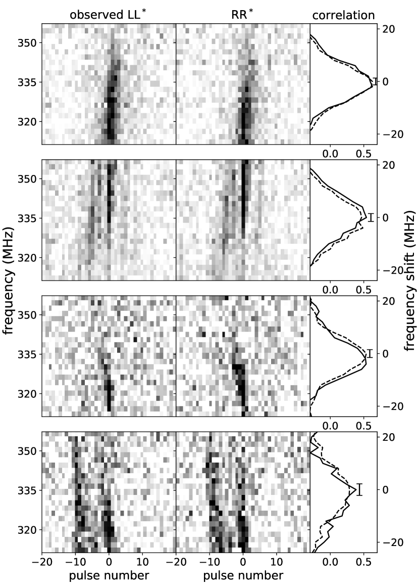
Figure 4: Spectra of four main pulse lensing events in left and right circular polarization. The images show the flux in 2 MHz bins for consecutive pulses, and the side panels show the cross polarization frequency correlation of the brightest pulse (number 0). The similarity of the spectra of the two polarizations sets strong limits on the strength of any magnetic field parallel to the line of sight.

4.1 Constraints from lensed pulses

We first constrain the parallel magnetic field using the spectra of the pulses magnified by plasma lenses in left and right circular polarization. Four of these pairs of spectra are shown in Figure 4. Here, we follow Main et al. (2018) and divide the spectra by average spectra from the surrounding 30 s to remove effects of interstellar scintillation (which is constant on these timescales, and identical for the two polarizations). From the figure, it is clear that the spectra of the two polarizations do not differ significantly; below, we discuss the resulting constraints on a uniform or small-scale magnetic field.

4.1.1 Medium and large-scale parallel magnetic fields

The presence of a uniform magnetic field in a lensing region will, as shown in section 3.1.2, generate a difference in focal frequency between left and right polarizations. To obtain the strongest constraint, we select the pulses with the strongest chromaticity across our band and cross-correlate the left and right polarized flux. Next, we determine the frequency offset by fitting a Gaussian to the cross correlation function, and an associated uncertainty from simulations, in which for each selected pulse we take the smoothed polarization-averaged frequency profile, add independent sets of random noises to simulate the two polarizations, and then find frequency offsets in the cross-correlation functions as for the real data. We take as the uncertainty for a given pulse the $68\%$ confidence interval in the offsets measured in 200 such simulations.

Inspecting the spectra, we find that the pulses are very similarly magnified in both polarizations (see Fig. 4): the auto and cross correlations of their spectra are equally strong and no statistically significant offset in the cross correlation is found. The $B_{\parallel}$ derived from the spectra are shown as triangles in Figure 3. Each magnified event constrains $B_{\parallel}$ on the scales of the lensing region to be smaller than 1 to 3 G. Averaging 51 events, we constrain any large-scale uniform magnetic field to $\overline{B}_{\parallel}=0.02\pm 0.09$ G, with a reduced $\chi^{2}=0.9$ — this is consistent with zero magnetic field.

4.1.2 Small-scale parallel magnetic field variations

Variations in magnetic field strength within the lensing regions will make it impossible for a lens to focus left and right circular the same way, and in Section 3.1.3 we found that even small changes in $B_{\parallel}$ would result in only a single polarization being magnified (see Figure 1). For all the detected lensing events,both polarizations are magnified, by amounts that are the same to within the uncertainties. Quantitatively, we infer that within those lenses, $\left\langle\Delta B_{\parallel}^{2}\right\rangle^{1/2}<10\,\mathrm{mG}$.

4.2 Constraints from giant pulses

PSR B1957+20 shows short, intrinsically bright giant pulses (Knight et al., 2006; Main et al., 2017), which are strongly polarized and can be used to provide independent measurements of the magnetic field.

The polarization properties of giant pulses vary from pulse to pulse. For magnetic field measurements, the best ones are those which are strongly linearly polarized and thus allow one to measure Faraday rotation. During the 7.2 hr observation away from eclipse, we found 28 suitable giant pulses, but unfortunately none of the giant pulses in the $\sim\!0.5$ hr near eclipse were similarly suitable. Therefore, we instead attempt to measure the Faraday delay of those giant pulses, which gives a complementary constraint to that derived by Fruchter et al. (1990) from profiles integrated over 10–60 s, in that it is sensitive also to magnetic fields that vary on much smaller scales. Furthermore, we use one bright giant pulse with strong circular polarization to constrain the perpendicular magnetic field.

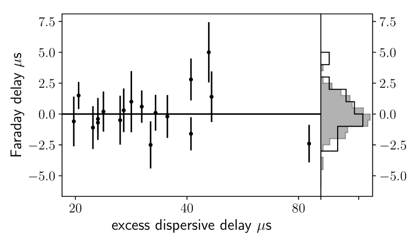
Figure 5: Faraday delay measured for individual giant pulses. Left: Delays $\tau_{F}$ for individual giant pulses near eclipse, as a function of the excess dispersive delay near them. No significant detections are made. Right: Delay histograms for giant pulses near (line) and away (grey, filled) from eclipse, showing that the distributions are the same within the uncertainties.

4.2.1 Medium and large-scale parallel magnetic fields

We measure the Faraday delay $\tau_{F}$ by cross-correlating giant pulse profiles in left and right circular polarizations, and fitting a Gaussian to the cross-correlation function. We perform the same bootstrap simulation as described in section 4.1.1 to obtain 1$\sigma$ error for the Faraday delay. We compare the simulated errors for GPs away from eclipses, where $\tau_{F}$ is expected to be 0, with the actual scattering of measured $\tau_{F}$ from the same group. The average simulated error is $\sigma=1.5\,\mu$s, and the scattering of measured $\tau_{F}$ is $\sigma=1.3\,\mu$s, which is consistent. For each GP, we measure the dispersive delay $\tau_{p}$ near it by fitting the regular pulse profile integrated over 2 s to the average pulse profile away from eclipse (enough to ensure the uncertainty, of $\sim\!0.5\,\mu$s, is small compared that for the time offset).

In Figure 5, we show the measured Faraday delay for all the GPs with excess dispersive delay $\tau_{p}>20\,\mu s$. As can be seen, no significant detections are made for any giant pulse, and indeed the distribution of the measured $\tau_{F}$ near eclipse is the same as that for the ones measured away from eclipse. The corresponding limits on the parallel magnetic field are $B_{\parallel}\lesssim 5$ G (see circles in the top panel of Figure 3). One also sees that the measured Faraday delay is not increasing with dispersive delay, as would be expected for a large-scale uniform magnetic field; averaging the constraints yields $\overline{B}_{\parallel}=-0.2\pm 0.3$ G. The data are thus consistent with $B_{\parallel}=0\,$G, with a reduced $\chi^{2}=0.9$ for N=18.

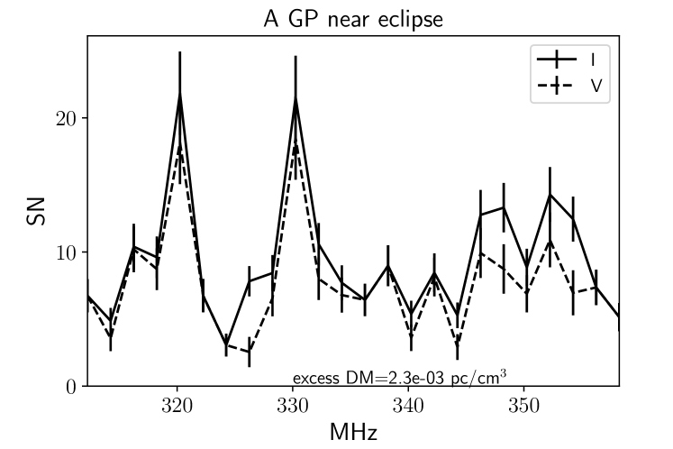
Figure 6: Spectrum of a giant pulse in a region of high excess dispersion measure, of $\sim\!10^{-3}\,\hbox{${\rm pc/cm}^{3}$}$. The pulse is strongly circularly polarized across the band, without any evidence of dips or sign changes due to generalized Faraday rotation.

4.2.2 Perpendicular magnetic field

We detect one bright giant pulse near eclipse, in the region with excess dispersion of $10^{-3}$${\rm pc/cm}^{3}$, which is strongly circularly polarized. As can be seen in Figure 6, the polarization is strong across the band, i.e., it is not depolarized by rapid generalized Faraday rotation around a natural axis close to the Poincaré sphere equator, as would be given the expected $\sim\!200$ turns expected across the band for a 20 G field (see Sec. 3.3). Indeed, the circular polarization does not change sign across the band, suggesting that the induced rotation changes by less than a cycle across the band, which strongly against a quasi-perpendicular magnetic field (for detailed discussion, see section 5.2).

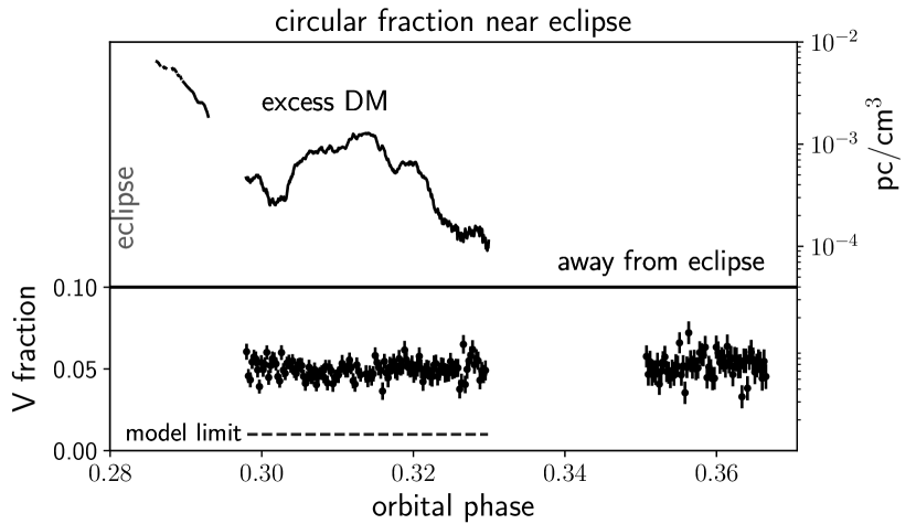
Figure 7: Circularly polarized fraction of the emission of the main pulse, averaged in 10 s bins. The fraction at large excess dispersion measure is consistent with that seen away from eclipse, unlike what would be expected if the eclipse region had a strong perpendicular magnetic field.

4.3 Constraints from the average pulse profile

The average pulse profile has a small circularly polarized component. If there were a perpendicular magnetic field that was much stronger than the parallel one, one would expect this to be reduced by generalized Faraday rotation. To look for this, we measured the cirularly polarized fraction for pulse profiles integrated over 10 s. We find that both near and away from eclipse, the circularly polarized fraction is $5\pm 1\%$, without any correlation with excess dispersion measure (see Fig. 7). This suggests no more than about most a turn across our band due to generalized Faraday rotation, which rules out the hypothesis of a quasi-perpendicular magnetic field (see also Sec. 5.2 below).

5 Implications

We described in Section 2 the theoretical arguments for expecting a strong, $\gtrsim\!20\,G$ magnetic field near the eclipse region, and gave three possible reasons for why, nevertheless, Fruchter et al. (1990) might have failed to detect such fields using Faraday delay in integrated pulse profiles. We discuss how our new constrains affect these scenarios.

5.1 Small-scale variations in magnetic field

The magnetic field could be as strong as expected, but organized in small loops, with radii of order $cP/2\approx 240$ km. In Section 4.1.1, however, we found that even for single magnified pulses, no effect of $B_{\parallel}$ is seen, and hence we exclude fields on spatial scales larger than those of the lenses, i.e., a few times the Fresnel scale. We also found that the field cannot vary much on scales or order of or smaller than the Fresnel scale, with $\sigma_{B_{\parallel}}=\langle\Delta B_{\parallel}^{2}\rangle^{1/2}<10\,\mathrm{mG}$ in the lensing region.

The reconnection loops can provide a net $B_{\parallel}$ of exactly zero spatially along the loop, but they will inevitably yield magnetic variance. Given previous constraints, the only way to obtain a low $B_{\parallel}$ was to average it down along the line of sight by having random orientations of the magnetic fields in different loops. Our new constraints on the magnetic field in small spatial structures imply that this cancellation has to be better than 10 mG for each line of sight. To average down $B_{\parallel}$ from $\sim\!10$ G to $\lesssim\!10$ mG, one would have to average over $\gtrsim\!10^{6}$ reconnection loops, well beyond the maximum of $\sim a/(cP/2)\sim 10^{3}$ reconnection loops that can reasonably be expected. The scenario of a highly varying large magnetic field thus becomes very unlikely at this point.

5.2 Perpendicular magnetic field

The low observed $B_{\parallel}$ could still be consistent with a strong, $\gtrsim\!20\,$G overall magnetic field if the field were nearly perpendicular to the LOS. In this case, the magnetic field would necessarily have a large scale, and by averaging our constraints given in Section 4.1.1, we found $B_{\parallel}=0.03\pm 0.09\,$G with reduced $\chi^{2}=1.0$ for all 69 measurements. To accommodate a 20 G magnetic field with parallel fraction smaller than $0.2\,$G, the angle $\alpha$ between $\vec{B}$ and the line of sight would have to be within $0.6^{\circ}$ of perpendicular. In this case, from Equations 12 and 14, $x\lesssim 0.3$ and $\theta\gtrsim 70^{\circ}$, i.e., the natural mode of the plasma is no longer circular but strongly elliptical.

Given excess dispersions between $10^{-4}$ and $10^{-3}\,\hbox{${\rm pc/cm}^{3}$}$ in the lensing region, one expects the Stokes parameters to rotate around the axis of the natural modes, with a number of cycles that differs by between 20 and 200 cycles across our 48 MHz bandwidth (see Sec. 3.3). This is enough to average down the polarization fraction perpendicular to the natural mode by at least an order of magnitude. For $\theta\gtrsim 70^{\circ}$, given that the circular and linear fraction away from eclipse are $V_{\mathrm{frac}}\sim\!5$% and $L_{\mathrm{frac}}<\!2\%$, respectively, one would thus expect an observed circular fraction near eclipse of $V_{\mathrm{frac}}^{\prime}<(V_{\mathrm{frac}}\cos(\theta)+L_{\mathrm{frac}}\sin(\theta))\cos(\theta)=1\%$. Since this is inconsistent with the measurements shown in Figure 7, we conclude that a large quasi-perpendicular magnetic field is not present in the interface.

5.3 Pair plasma

If the excess dispersion measure is due not just to electrons, but reflects an electron-positron pair plasma, then the effects of a parallel magnetic field will cancel, because electrons and positrons cause Faraday rotation in opposite directions. A pair plasma could not, however, conceal a perpendicular magnetic field, because the gyro motions of electrons and positrons along such a field project in the same way on the linear polarization of light, i.e., for both the phase velocity of the ‘o’ mode is that of an unmagnetized plasma, while that of the ‘x’ mode is not as strongly affected. Hence, the natural modes for a pair plasma are two linear polarizations, which are identical to what one would find if one had just electrons in a completely perpendicular magnetic field (Melrose, 1997).

Given the above, for a magnetized pair plasma one expects the Stokes parameters of the incoming wave to rotate around a natural axis located in the equator of the Poincaré sphere 2. From Equation 16, assuming a 20 G magnetic field at 30^∘ from the line of sight (i.e., $B_{\perp}=10\,$G), one expects rotations by 10 to 100 cycles across the band, again strongly suppressing the circularly polarized fraction, in contrast to what we observe. For a pair plasma, the only solution would seem to assume a largely parallel magnetic field, such that $B_{\perp}\lesssim 0.1\,$G. This seems contrived.

6 Ramifications

In this paper, we have demonstrated that birefringence in plasma lenses can be used to measure the parallel magnetic field $B_{\parallel}$ and to constrain small-scale variations in that field. We attempted to do so for the Black Widow Pulsar B1957+20, where $B\gtrsim 20$ G is expected at the interface between the pulsar wind and its companion, but found only upper limits, which are inconsistent with the presence of such a strong field, even if it were to vary rapidly in orientation.

We also found that other scenarios to conceal a large magnetic field, such as placing it nearly perpendicular to the line of sight, or assuming that the excess dispersion is caused by a pair plasma, seem excluded as well, as they would predict changes in the fraction of circular polarization that are not observed. Given these new constraints, the long eclipse and the large stand-off distance of the companion wind are very puzzling.

Birefringence in plasma lensing could be applied to other systems in which plasma lensing has been seen or suspected. For instance, the binary pulsar PSR J1748-2446A also shows magnified events near eclipse (Bilous et al., 2011). It would also be interesting to look for further systems, in particular ones such as PSR J1748-2446 and PSR J2256-1024 in which changes in RM and/or depolarization are observed near eclipse You et al. (2018); Crowter (2018). Furthermore, Fast Radio Bursts might be good targets, as they have been proposed to be lensed by plasma in their local galaxies (Cordes et al., 2017). Indeed, the spectra of the only repeating FRB so far, FRB 121102, look similar to the lensing spectra of B1957+20 (Spitler et al., 2016; Farah et al., 2018; Main et al., 2018), and their strong chromaticity should make it relatively easy to detect the frequency offsets resulting from birefringence. Furthermore, a dynamic magneto-ionic environment has been inferred for FRB 121102 (Michilli et al., 2018) and it is fairly clear that other FRBs are observed to pass through dense magnetized plasma in their host galaxy (e.g., FRB 110523; Masui et al. 2015). If birefringence is found, it would provide direct proof that FRBs are affected by lensing, and would give a local measurement of the field strength (unlike a Rotation Measure, which is integrated along the line of sight).

Appendix A Simulation with birefringence

We demonstrate the effects of birefringence in plasma lens with a simple simulation, in which we assume one-dimensional variations in dispersion measure, and aim to mimic the conditions found in PSR B1957+20. We start by generating a randomly varying dispersion measure phase screen $\Phi_{\text{DM}}$, ensuring that at large scales we match the observed power spectrum $P_{\text{DM}}(q)$ of excess DM in the egress of the eclipse. Here, we assume a flow velocity three times the orbital velocity to convert timescales on which we measure dispersion measure to spatial scales $1/q$ – an arbitrarily selection within the constraints from Main et al. (2018) to make simulated spectra look like real spectra. With this choice, and imposing an inner scale cutoff at $q_{\text{in}}$ in the power spectrum in order for the strong magnification to appear, we obtain output spectra that resemble observed ones. Specifically, $\Phi_{\text{DM}}$ is computed as

$$\Phi_{\text{DM}}(x)=\text{FT}^{-1}\left[2\pi(u_{q}+iv_{q})\sqrt{P_{\text{DM}}(q)}\exp\left(-\frac{q^{2}}{2q_{\text{in}}^{2}}\right)\right]$$ (17)

where FT is the Fourier transform and $u_{q}$ and $v_{q}$ are normally distributed random variables with unit variance. For Fig 1, we used $1/q_{\mathrm{in}}\sim 7600$ km, a relatively large inner scale cutoff in order to see enough strong lenses in short simulation time, and $P_{\mathrm{DM}}(q)\sim 1.3\cdot 10^{-9}q^{-2.0}$ to measure the observed DM distribution.

At each point of the phase screen, we add a magnetic field contribution $\Phi_{B}=\Phi_{\mathrm{DM}}(x)f_{B_{\parallel}}(x)/f$ (with $f_{B_{\parallel}}(x)$ reflecting a choice of magnetic field distribution), and then compute the received electric field using the Fresnel-Kirchhoff integral (Born & Wolf, 1980):

$$E_{r}(f,x_{s})=\frac{e^{-i\pi/4}}{R_{\text{Fr}}}\int dx\exp\left(2\pi i\left[\Phi_{\text{GM}}+\Phi_{\text{DM}}(x)\pm\Phi_{B}(x)\right]\right)$$ (18)

where $f$ is the observed frequency and $x_{s}$ is the position of the pulsar in the source plane.

For Figure 1, we selected a particular time when a clear caustic formed, and then reran the inverse Fourier transform twice, once adding a uniform magnetic field and once one that had a gradient.

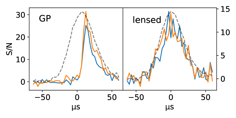
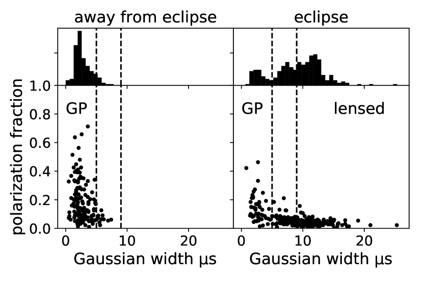
Figure 8: Separating lensed and giant pulses. Top: The profiles of a main pulse magnified by a plasma lens and a giant pulse appearing at similar phase during the egress of the eclipse, in left and right circular polarization (colour lines), with the average profile integrated over the surrounding 8 s overdrawn (dashed, scaled to match in amplitude). Bottom: Polarized fraction and widths of strong pulses far and near eclipse, with the width inferred from fitting a Gaussian convolved with an exponential with fixed timescale. We consider pulses with fitted Gaussian width below $5\,\mu$s to be giant pulses and those with widths above $9\,\mu$s to be lensed ones (as indicated by the two vertical lines). Note that giant pulses can be highly polarized, while lensed pulses are not.

Appendix B Separating lensed and giant pulses

In the region where the excess dispersion exceeds $10^{-4}\,\hbox{${\rm pc/cm}^{3}$}$, we detect 268 pulses at $\mathrm{SN}>20$ in the main pulse phase, which corresponds to magnification of $>10$. The brightest pulses clearly draw from two populations (Figure 8, top panel): one in which the widths are similar to that of the average main pulse profile – these are lensed and only appear near eclipse – and another in which the pulses have narrow exponential profiles – which appear randomly at all orbital phases. Clearly, the first group consist of lensed pulses, while the latter are giant pulses.

Since away from eclipse, all the bright pulses are giant pulses, we can use the properties of those pulses as a reference in separating giant and lensed pulses. To obtain a quantative measure of pulse width, we fit the profiles of all single strong pulses we detect with a Gaussian of variable amplitude and width convolved with an exponential function that has its timescale fixed to the scattering time of $12.2\,\mu$s measured by Main et al. (2017).

As shown in Figure 8 (lower panel), the fitted widths for pulses away from eclipse are all below $9\,\mu$s, and the majority of them are below $5\,\mu$s. Typically, they are strongly polarized (unlike the regular pulse emission, which is nearly unpolarized; Fruchter et al. 1990). For the bright pulses near eclipse, in constrast, a much broader distribution is found, with a clear set of short, polarized pulses and another one of wider, low-polarization pulses. We identify the pulses with width $<5\,\mu$s as giant pulses, and those with width $>9\,\mu$s and low polarization fraction as lensed pulsed. For pulses with intermediate widths, we cannot exclude that some are giant pulses, and hence we did not include them in our analysis.

References

- Arzoumanian et al. (1994) Arzoumanian Z., Fruchter A. S., Taylor J. H., 1994, ApJ, 426, 85
- Astropy Collaboration et al. (2013) Astropy Collaboration et al., 2013, A&A, 558, A33
- Berdyugina et al. (2017) Berdyugina S. V., Harrington D. M., Kuzmychov O., Kuhn J. R., Hallinan G., Kowalski A. F., Hawley S. L., 2017, ApJ, 847, 61
- Bilous et al. (2011) Bilous A. V., Ransom S. M., Nice D. J., 2011, in Burgay M., D’Amico N., Esposito P., Pellizzoni A., Possenti A., eds, American Institute of Physics Conference Series Vol. 1357, American Institute of Physics Conference Series. pp 140–141, doi:10.1063/1.3615100
- Born & Wolf (1980) Born M., Wolf E., 1980, Principles of Optics Electromagnetic Theory of Propagation, Interference and Diffraction of Light
- Cordes et al. (2017) Cordes J. M., Wasserman I., Hessels J. W. T., Lazio T. J. W., Chatterjee S., Wharton R. S., 2017, ApJ, 842, 35
- Crowter (2018) Crowter K., 2018, PhD thesis, University of British Columbia, doi:http://dx.doi.org/10.14288/1.0371173, https://open.library.ubc.ca/collections/ubctheses/24/items/1.0371173
- Farah et al. (2018) Farah W., et al., 2018, MNRAS,
- Fruchter et al. (1988) Fruchter A. S., Stinebring D. R., Taylor J. H., 1988, Nature, 333, 237
- Fruchter et al. (1990) Fruchter A. S., et al., 1990, ApJ, 351, 642
- Kaplan et al. (2013) Kaplan D. L., Bhalerao V. B., van Kerkwijk M. H., Koester D., Kulkarni S. R., Stovall K., 2013, ApJ, 765, 158
- Kennett & Melrose (1998) Kennett M., Melrose D., 1998, Publ. Astron. Soc. Australia, 15, 211
- Knight et al. (2006) Knight H. S., Bailes M., Manchester R. N., Ord S. M., Jacoby B. A., 2006, ApJ, 640, 941
- Mahajan et al. (2018) Mahajan N., van Kerkwijk M. H., Main R., Pen U.-L., 2018, preprint, p. arXiv:1807.01713 (arXiv:1807.01713)
- Main et al. (2017) Main R., van Kerkwijk M., Pen U.-L., Mahajan N., Vanderlinde K., 2017, ApJ, 840, L15
- Main et al. (2018) Main R., et al., 2018, Nature, 557, 522
- Masui et al. (2015) Masui K., et al., 2015, Nature, 528, 523
- Melrose (1997) Melrose D. B., 1997, Plasma Physics and Controlled Fusion, 39, A93
- Michilli et al. (2018) Michilli D., et al., 2018, Nature, 553, 182
- Ryba & Taylor (1991) Ryba M. F., Taylor J. H., 1991, ApJ, 380, 557
- Schneider et al. (1992) Schneider P., Ehlers J., Falco E. E., 1992, Gravitational Lenses, doi:10.1007/978-3-662-03758-4.
- Spitler et al. (2016) Spitler L. G., et al., 2016, Nature, 531, 202
- Steiner et al. (2015) Steiner A. W., Gandolfi S., Fattoyev F. J., Newton W. G., 2015, Phys. Rev. C, 91, 015804
- Stovall et al. (2014) Stovall K., et al., 2014, ApJ, 791, 67
- Thompson et al. (1994) Thompson C., Blandford R. D., Evans C. R., Phinney E. S., 1994, ApJ, 422, 304
- Tuntsov et al. (2016) Tuntsov A. V., Walker M. A., Koopmans L. V. E., Bannister K. W., Stevens J., Johnston S., Reynolds C., Bignall H. E., 2016, ApJ, 817, 176
- You et al. (2018) You X. P., Manchester R. N., Coles W. A., Hobbs G. B., Shannon R., 2018, preprint, p. arXiv:1809.01309 (arXiv:1809.01309)
- van Kerkwijk et al. (2011) van Kerkwijk M. H., Breton R. P., Kulkarni S. R., 2011, ApJ, 728, 95