Controlling decoherence speed limit of a single impurity atom
in a Bose-Einstein-condensate reservoir

Abstract

We study the decoherence speed limit (DSL) of a single impurity atom immersed in a Bose-Einstein-condensed (BEC) reservoir when the impurity atom is in a double-well potential. We demonstrate how the DSL of the impurity atom can be manipulated by engineering the BEC reservoir and the impurity potential within experimentally realistic limits. We show that the DSL can be controlled by changing key parameters such as the condensate scattering length, the effective dimension of the BEC reservoir, and the spatial configuration of the double-well potential imposed on the impurity. We uncover the physical mechanisms of controlling the DSL at root of the spectral density of the BEC reservoir.

I Introduction

Quantum coherence is the essential reason for quantum counterintuitive features that challenge our classical perception of nature, and long coherence time is a crucial condition for the viability of performing quantum information processing. However, the unavoidable couplings between quantum systems and their reservoirs induce the phenomenon of quantum decoherence Breuer2002 . Developing a quantitative understanding of the decoherence mechanism and exploring controllable methods of decoherence Leggett1987 ; Prokof2000 ; Kuang1999-1 ; Kuang1995 ; Kuang1999-2 ; Liao2011 ; Yuan2010 ; Lu2010 ; He2017 are therefore critical. In recent years, much attention has been paid to the realization of long-lived quantum coherence. But few works focus on the lower bound of coherence time, and how to regulate the lower bound of coherence time still remains an open question. The aim of this paper is to address this problem making use of quantum speed limit (QSL) for a single impurity atom in a Bose-Einstein-condensed (BEC) reservoir.

The QSL time, denoted by $\tau_{QSL}$, is defined as the minimal time between two distinguishable states of a quantum system. It can be used to characterize the ultimate bound imposed by quantum mechanics on the maximal evolution speed. Recently, based on various distance metrics of two distinguishable states or the notion of quantumness, different bounds on the $\tau_{QSL}$ for both isolated Mandelstam1945 ; Margolus1998 ; Vittorio2003 and open Taddei2013 ; Campo2013 ; Sebastian2013 ; Deffner02017 ; Diego2016 ; Cimmarusti2015 ; Jones2010 ; Zhang2014 ; Sun2015 ; Mirkin2016 ; Xu2016 ; Meng2015 ; Song2016 ; Song2017 ; Deffner2017 ; Campaioli2018 ; Mo2017 ; Lee2018 system dynamics have been obtained. In this paper, we adopt the $\tau_{QSL}$ derived by Taddei et al, who use quantum Fisher information for time estimation and choose Bures fidelity as the distance measure between two quantum states. For a given distance, a shorter $\tau_{QSL}$ implies a higher dynamical speed upper bound, otherwise, longer $\tau_{QSL}$ means a lower dynamical speed limit. As for a quantum pure dephasing model, the $\tau_{QSL}$ is exactly the lower bound of coherence time, and it can be used to characterize the upper bound of quantum decohering speed, i.e., the quantum decoherence speed limit (DSL).

Here we consider a single impurity atom immersed in a BEC. The impurity atom is confined by a deep, symmetric double well potential, while the BEC atoms are confined by a very shallow trapping potential. In Refs. Bloch2008 ; Cirone2009 ; Haikka2011 ; Klein2007 ; Yuan2017 , it has been proved that the BEC atoms can be used to simulate a phase damping reservoir for the doped impurity atom. Meanwhile, BEC systems are essentially macroscopic quantum many body systems with effectively controllable dimension and nonlinear interaction. These provide us with a platform to control the decoherence of the single impurity atom by the use of the nonlinear BEC reservoir with different dimensions. Here we mainly consider the effect of these controllable parameters of the BEC reservoir on the impurity's lower bound of coherence time, i.e., quantum DSL. We show that not only the nonlinearity and the dimension of the BEC, but also the spatial form of the double well potential imposed on the impurity can be all treated as controllable parameters to manipulate the impurity's lower bound of coherence time. And in order to insight the physical mechanism behind the control, we also analyze the spectral density in details. We find that the nonlinear interaction and the effective dimension of the BEC can change the spectral density from a soft subohmic spectrum to a hard superohmic spectrum, while the characteristic length of each well and the distance between two wells of the double well potential change the cut-off frequency and the effective coupling constant in the spectral density, respectively.

The paper is organized as follows. In Sec. II, we introduce our physical model and obtain the dynamics of the impurity in the dephasing BEC reservoir. In Sec. III, we investigate the possibility of manipulating the quantum DSL of the impurity atom by various controllable parameters such as the nonlinearity and the effective dimension of the BEC reservoir, and the spatial parameters of double well potential imposed on the impurity. Finally, Sec. IV is devoted to some conclusions.

II Physical model and decoherence analysis

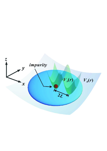
Figure 1: Schematic of the impurity coupled to a quasi-two-dimensional BEC environment. The impurity atom (red circle) is trapped in a double well potential $V_{A}(\textbf{r})$ with the distance between two wells $2L$, while the BEC (blue region) is confined in a shallow harmonic trap $V_{B}(\textbf{r})$.

We consider an impurity atom immersed in a BEC. As shown in Fig. 1, the BEC is confined by a very shallow trapping potential $V_{B}(\textbf{r})$, while the impurity atom is trapped by a deep, symmetric double well potential $V_{A}(\textbf{r})$ with the distance between two wells $2L$. Here the occupations of the impurity in the left and the right well represent two pseudo-spin states, denoted by $|g\rangle\equiv|L\rangle$ and $|e\rangle\equiv|R\rangle$, respectively. Assume that the double well is separated by a high-energy barrier, the tunneling between the two wells can be neglected. At low energies, only the contact interaction between the impurity and the BEC atoms contributes significantly. Then the BEC atoms could serve as a ground for simulating a phasing damping environment for the doped impurity atom. The Hamitonian of the impurity-BEC system takes the form of an effective spin-boson model Cirone2009 ; Haikka2011 ($\hbar=1$),

$$\hat{H}_{\rm{eff}} = \omega_{0}\hat{\sigma}_{z}+\sum_{\mathbf{k}}\omega_{\mathbf{k}}\hat{a}_{\mathbf{k}}^{\dagger}\hat{a}_{\mathbf{k}}+\hat{\sigma}_{z}\sum_{\mathbf{k}}\left(\xi_{\mathbf{k}}\hat{a}_{\mathbf{k}}^{\dagger}+\xi_{\mathbf{k}}^{\ast}\hat{a}_{\mathbf{k}}\right),$$ (1)

where $\sigma_{z}=|R\rangle\langle R|-|L\rangle\langle L|$, $\omega_{0}$ is the effective energy difference between the two pseudo-spin states of the impurity, and $\hat{a}_{\mathbf{k}}^{\dagger}(\hat{a}_{\mathbf{k}})$ is the creation (annihilation) operator of the Bogoliubov phonon of the BEC on the top of condensate wave function with the energy $\omega_{\mathbf{k}}$ Lifshitz1980 ; Ohberg1997 , and $\xi_{\mathbf{k}}$ is the coupling constant between the impurity and the BEC.

The BEC excitations obey the following dispersive relation

$$\omega_{\mathbf{k}} = \sqrt{2\epsilon_{\mathbf{k}}n_{D}g_{D}+\epsilon_{\mathbf{k}}^{2}},$$ (2)

where the subscript $D$ denotes the effective dimension of the BEC, $n_{D}$ is the condensate number density, $g_{D}$ is the inter-atomic nonlinear coupling constant, and $\epsilon_{\mathbf{k}}=\frac{k^{2}}{2m_{B}}$ is the free-particle energy with the mass of a background gas particle $m_{B}$ and the momentum $k=|\mathbf{k}|$. It is worth noting that from Eq. (2) we can obtain two interesting limit cases of the dispersive relation Cirone2009 ; Zhou ; Guo . The first is the phonon-like type dispersive relation $\omega_{\mathbf{k}}\propto k$, which happens in the regime of low-energy excitations $\epsilon_{\mathbf{k}}\ll 2n_{D}g_{D}$ or strong nonlinear interaction $g_{D}\gg\epsilon_{\mathbf{k}}/2n_{D}$. The second is the free-particle type dispersive relation $\omega_{\mathbf{k}}\propto\epsilon_{\mathbf{k}}$, which occurs in the regime of high-energy excitations or when the inter-atomic nonlinear interaction can be ignored.

Under the harmonic approximation through calculating the analytical expression of the ground state wave function of the impurity in each well, we can get the coupling constant between the impurity and the BEC Cirone2009 ; Haikka2011

$$\xi_{\mathbf{k}}=-i\eta_{D}\sqrt{\frac{n_{D}\epsilon_{\mathbf{k}}}{V\omega_{\mathbf{k}}}}e^{-k^{2}\sigma^{2}/4}\sin\left(\mathbf{k}\cdot\mathbf{L}\right)e^{-i\mathbf{k}\cdot\mathbf{r}_{W}},$$ (3)

where $\eta_{D}$ is the coupling constant of the impurity-BEC contact interaction with volume $V$, $\mathbf{r}_{W}$ is the center coordinate of the double well potential $V_{A}(\textbf{r})$, and $\sigma=\frac{\hbar}{\sqrt{m_{A}\omega}}$ is the characteristic length of two approximate harmonic wells of $V_{A}(\textbf{r})$ with the trapping frequency $\omega$ and the mass of the impurity $m_{A}$.

Note that, by changing the shape of the trapping potentials, it is possible to produce dilute gases in highly anisotropic configurations, where the motion of BEC atoms is quenched in quasi-one-dimensional (1D) or quasi-two-dimensional (2D) directions Pitaevskii2003 ; Naidon2007 ; Hangleiter2015 ; Naidon2006 ; Catani2012 ; Bloch2008 . The consequent inter-atomic interaction strengths ( $g_{1}$ and $g_{2}$) in 1D and 2D BEC can be expressed in terms of the inter-atomic interaction strength ($g_{3}$) in 3D BEC

$$g_{1}=\frac{g_{3}}{2\pi a_{\perp,B}^{2}},\hskip 14.22636ptg_{2}=\frac{g_{3}}{\sqrt{2\pi}a_{z,B}},\hskip 14.22636ptg_{3}=\frac{4\pi a_{B}}{m_{B}},$$ (4)

where $a_{B}$ is the tunable $s$-wave scattering length of the BEC. $a_{\perp,B}$ and $a_{z,B}$ are the transversal width and the axial length of the wave function of the BEC atoms, respectively.

Similarly, one can obtain the number densities of the 1D and 2D BEC with $n_{3}$ being the number density of the 3D BEC Pitaevskii2003 ; Bloch2008

$$n_{1}=\pi n_{3}a_{\perp,B}^{2},\hskip 14.22636ptn_{2}=\sqrt{\pi}n_{3}a_{z,B}.$$ (5)

And the 1D and 2D impurity-BEC coupling constants are expressed as

$$\eta_{1}=\frac{\eta_{3}}{\pi(a_{\perp,A}^{2}+a_{\perp,B}^{2})},\eta_{2}=\frac{\eta_{3}}{\sqrt{\pi(a_{z,A}^{2}+a_{z,B}^{2})}},\eta_{3}=\frac{2\pi a_{AB}}{m_{AB}},$$ (6)

where $a_{\perp,A}$ is the transversal width of $V_{A}(\textbf{r})$ for the 1D case, and $a_{z,A}$ is the axial length for the 2D case. $a_{AB}$ is the $s$-wave scattering length for impurity-BEC collisions and $m_{AB}=\frac{m_{A}m_{B}}{m_{A}+m_{B}}$ is the reduced mass.

For the sake of simplicity, we consider the case that the BEC reservoir is at zero-temperature. Assume that the qubit is initially in an arbitrary state $\hat{\rho}\left(0\right)=\frac{1}{2}(\mathbb{I}+x\sigma_{x}+y\sigma_{y}+z\sigma_{z})$. In the interaction picture with respect to $\hat{H}_{0}=\omega_{0}\hat{\sigma}_{z}+\sum_{\mathbf{k}}\omega_{\mathbf{k}}\hat{a}_{\mathbf{k}}^{\dagger}\hat{a}_{\mathbf{k}}$, the exact reduced impurity dynamics can be obtained by using Magnus expansion Blanes2009 with the following expression

$$\hat{\rho}\left(t\right)=\frac{1}{2}\left(\begin{array}[]{cc}1+z&(x-iy)e^{-\Gamma\left(t\right)}\\ (x+iy)e^{-\Gamma\left(t\right)}&1-z\end{array}\right),$$ (7)

where the dephasing function $\Gamma\left(t\right)$ Cirone2009 ; Haikka2011 is given by,

$$\Gamma\left(t\right) = \frac{8\eta_{D}^{2}n_{D}}{\left(2\pi\right)^{D}}\int dkk^{D-1}f_{D}(kL)\frac{e^{-k^{2}\sigma^{2}/2}\sin^{2}\left(\omega_{\mathbf{k}}t/2\right)}{\omega_{\mathbf{k}}\left(2n_{D}g_{D}+\epsilon_{\mathbf{k}}\right)}.$$ (8)

During the calculation of $\Gamma(t)$, we have used the continuum limit $\frac{1}{V}\sum_{\mathbf{k}}\rightarrow\frac{1}{\left(2\pi\right)^{D}}\int d\Omega_{D}\int dkk^{D-1}$. The angular integral is defined as $f_{D}(kL)=\int d\Omega_{D}\sin^{2}\left(\mathbf{k}\cdot\mathbf{L}\right)$ with $\Omega_{D}$ being the surface of the unit sphere in $D$ dimensions. It is not difficult to find that the angular integrals read as $f_{1}(kL)=\sin^{2}(kL)$, $f_{2}(kL)=\pi[1-J_{0}(2kL)]$ with $J_{0}(x)$ being the Bessel function of the first kind, and $f_{3}(kL)=2\pi[1-\frac{\sin(2kL)}{2kL}]$. Up to now, the dephasing function of the impurity atom in the $D$-dimensional BEC environment can be obtained by combining Eqs. (2),(8). Significantly, the dephasing function $\Gamma(t)$ is not only related to the impurity-BEC coupling constant $\eta_{D}$, but also can be modulated by the boson-boson s-wave scattering length $a_{B}$ through $g_{D}$, the effective dimension $D$ of the BEC reservoir, as well as the spatial form of the double well potential $V_{A}(\textbf{r})$, including the parameters $\sigma$ and $L$.

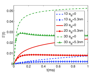
Figure 2: (Color online) Comparison of the dynamical behaviors of the dephasing function $\Gamma(t)$ in free and interacting BEC reservoirs with different dimensions. The blue dashed (with empty rhombus) line represents the free (interacting) $1$D case, the red solid (with empty circles) line represents the free (interacting) $2$D case, and the green dot-dashed (with empty triangle) line represents the free (interacting) $3$D case. Here the value of $a_{B}$ takes its nature value without using Feshbach resonances, $a_{B}=a_{NV}=5.3nm$, for the interacting case. Other parameters are given by $n_{3}=10^{20}m^{-3}$, $m_{B}=14.45\times 10^{-26}kg$, $m_{AB}=3.02\times 10^{-26}kg$, $a_{\bot,A}=a_{\bot,B}=100a_{NV}$, $a_{z,A}=a_{z,B}=100a_{Rb}$, $\sigma=45nm$, $L=150nm$, $a_{AB}=55a_{0}$ with the Bohr radius $a_{0}$.

Fig. 2 indicates the dependence of the dephasing function $\Gamma(t)$ on the effective dimension $D$ and the scattering length $a_{B}$ of the BEC atoms. Here the kind of atoms for the impurity is ${}^{23}Na$ with the mass $m_{A}\approx 3.82\times 10^{-26}kg$, while the kind of atoms for the BEC is ${}^{87}Rb$ with the mass $m_{B}\approx 14.45\times 10^{-26}kg$. One can create a low-dimensional background BEC by a suitable modification of the potential $V_{B}(\textbf{r})$. And the scattering length $a_{B}$ of the background ${}^{87}Rb$ condensate gas can be tuned via Feshbach resonances. Other parameters are given in the legend of Fig. 2 Cirone2009 ; Haikka2011 ; Jaksch1998 . As shown in the Fig. 2, for the case of free bosons in BEC, i.e., $a_{B}=0$, the $\Gamma(t)$ monotonically increases with the time in both the 1D and 2D BEC reservoirs. However, the $\Gamma(t)$ first increases and then trends to a constant value in the 3D BEC reservoir. These results indicate that the impurity would completely dephase in the long-time limit for both the 1D and 2D cases, but there exists a stationary coherence for the 3D case. As for the case of presence of inter-atomic interaction in the BEC reservoir, where the scattering length $a_{B}$ takes its natural value $a_{Rb}\approx 5.3nm$, the $\Gamma(t)$ falls down after it ascends first, and finally tends to be stable for three kinds of dimensions. That is to say, the inter-boson interaction or the nonlinearity of BEC reservoir induces the appearance of the stationary coherence of the impurity. And by comparing the dynamics of $\Gamma(t)$ in different dimension cases, we can find that the coherence of the impurity would also be enhanced by decreasing the effective dimension of the BEC reservoir.

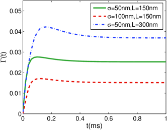
Figure 3: (Color online) The dynamics of dephasing function $\Gamma_{3}(t)$ in $3$D BEC reservoir for different spatial parameters of the double-well. The green solid line represents $\sigma=50nm,L=150nm$, the red dashed line represents $\sigma=100nm,L=150nm$, and the blue dot-dashed line represents $\sigma=50nm,L=300nm$. The scattering length of the background BEC takes its nature value of $a_{B}=a_{NV}=5.3nm$. Other parameters are the same as in Fig. 2.

We now turn to investigate the influence of the spatial configuration of the double well $V_{A}(\textbf{r})$, including the parameters $\sigma$ and $L$, on the dephasing function $\Gamma(t)$. Here $\sigma=\sqrt{\frac{\hbar}{m_{A}\omega}}$ is the characteristic length with $\omega$ being the trapping frequency of the harmonic trap approximating the lattice potential at bottom of the left and the right wells. $L$ is the half of the distance between two wells of $V_{A}(\textbf{r})$. Both of them can be adjusted experimentally. Inspecting Fig. 3 we can find that for a given inter-atomic interaction $a_{B}$, the dephasing function in the $3$D BEC reservoir $\Gamma_{3}(t)$ decreases with increasing $\sigma$ or shortening $L$. This means that the larger $\sigma$ or smaller $L$ could induce the slower dephasing speed, and we find these results are also applicative for the low-dimension cases. In addition, comparing Figs. 2 with  3 one can conclude that the stationary coherence is much sensitive to the nonlinearity parameter $a_{B}$ of the BEC reservoir rather than the spatial parameters $\sigma$ and $L$ of the double well $V_{A}(\textbf{r})$. Anyway, these results provide us a way to control the quantum dephasing speed of the impurity atom in its BEC reservoir.

III control of the decoherence speed limit

In this section, we show how to manipulate the DSL of the impurity atom through changing controllable parameters of the impurity atom and the BEC reservoir. As was mentioned in the introduction section, the DSL can be characterized by the QSL time $\tau_{QSL}$. For a given distance $\mathcal{D}$ between two distinguishable states, a longer $\tau_{QSL}$ indicates a slower decohering limit speed, which means the greater robustness of the impurity against dephasing induced by the interaction with the BEC reservoir.

We now consider the DSL of the impurity atom between two quantum states with a distance $\mathcal{D}$. The authors in Ref. Taddei2013 have proved that the distance between the initial states $\hat{\rho}(0)$ and the final states $\hat{\rho}(\tau)$ is bounded by

$$\mathcal{D}\equiv\arccos\sqrt{F_{B}\left[\hat{\rho}(0),\hat{\rho}(\tau)\right]}\leq\frac{1}{2}\int_{0}^{\tau}\sqrt{\mathcal{F}_{Q}(t)}\ dt,$$ (9)

where the distance between two states is defined based on the Bures fidelity $F_{B}\left[\hat{\rho}(0),\hat{\rho}(\tau)\right]=\left[\mathrm{tr}\sqrt{\hat{\rho}(0)^{1/2}\hat{\rho}(\tau)\hat{\rho}(0)^{1/2}}\right]^{2}$, and $\mathcal{F}_{Q}(t)$ is the quantum Fisher information with respect to the time which can be expressed as Helstrom1976

$$\mathcal{F}_{Q}\left(t\right)=\sum_{m,n=\pm}\frac{2}{p_{m}+p_{n}}\left|\left\langle\psi_{m}\right|\frac{\partial\hat{\rho}(t)}{\partial t}\left|\psi_{n}\right\rangle\right|^{2}.$$ (10)

where $p_{\pm}$ ($\left|\psi_{\pm}\right\rangle$) are the eigenvalues (eigenstates) of the quantum state of the impurity atom. For the density operator of the impurity atom given by Eq. (7) we have

$$\left|\psi_{\pm}\right\rangle = N_{\pm}\left[(x-iy)e^{-\Gamma(t)}\left|e\right\rangle\mp(A\pm z)\left|g\right\rangle\right],$$

$$p_{\pm} = \frac{1}{2}\left(1\mp A\right)$$ (11)

where we have introduced the following functions

$$N_{\pm}^{-2}=2A(A\pm z),\hskip 14.22636ptA=\sqrt{(x^{2}+y^{2})e^{-2\Gamma\left(t\right)}+z^{2}}.$$ (12)

Submitting Eqs. (III) and (12) into Eq. (10), we can obtain the quantum Fisher information with respect to the time,

$$\mathcal{F}_{Q}\left(t\right)=\frac{\left(1-z^{2}\right)(x^{2}+y^{2})\dot{\Gamma}^{2}(t)e^{-2\Gamma\left(t\right)}}{1-z^{2}-(x^{2}+y^{2})e^{-2\Gamma(t)}}.$$ (13)

Thus, the upper bound of the distance $\mathcal{D}_{UB}$ between two distinguishable states can be obtained by inserting Eq. (13) into Eq. (9),

$$\mathcal{D}_{UB}=\frac{1}{2}\int_{0}^{\tau}\frac{\sqrt{(1-z^{2})(x^{2}+y^{2})}\left|\dot{\Gamma}(t)\right|e^{-\Gamma(t)}}{\sqrt{1-z^{2}-(x^{2}+y^{2})e^{-2\Gamma(t)}}}dt$$ (14)

From Eq. (14) we can see that the initial zero coherence $C\left[\rho(0)\right]\equiv x^{2}+y^{2}=0$ would lead to $\mathcal{D}_{up}=0$ at any time. In other words, the above bound consistently guarantees that the eigenstates of $\sigma_{z}$ do not evolve. Furthermore, assuming the initial states of the impurity $\hat{\rho}(0)$ are pure states, the bound saturates, i.e., $\mathcal{D}=\mathcal{D}_{UB}$, if and only if the $\hat{\rho}(0)$ is on the equator of the bloch sphere with $x^{2}+y^{2}=1$ and the first derivative of the dephasing function versus time $\dot{\Gamma}\left(t\right)>0$ within the driving time $t\in[0,\tau]$, which can be proved to be a Markovian process Taddei2013 . Noting that the bound saturation implies the dephasing channel connecting two states along a geodesic path. More importantly, Eq. (14) clearly shows that the $\mathcal{D}_{UB}$ for a given driving time $\tau$ is not only determined by the initial-state parameters ($x$, $y$, $z$), but also determined by the dephasing function $\Gamma(t)$ in Eq. (8) and its first derivative versus time $\dot{\Gamma}(t)$. In fact, the dependence of the $\mathcal{D}_{UB}$ on the effective dimension $D$ of the BEC, the boson-boson scattering length $a_{B}$, and the spatial form of the double-well potential (i.e., $\sigma$, $L$) is exactly from the dephasing function $\Gamma(t)$.

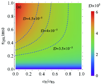
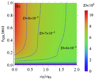
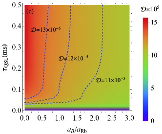
Figure 4: (Color online) The distance $\mathcal{D}$ as a function of the scattering length $a_{B}$ and the QSL time $\tau_{QSL}$. The blue dashed contour mark the dependence of the QSL time $\tau_{QSL}$ on the scattering length $a_{B}$ for given distances $\mathcal{D}$. From top to bottom, the three subfigures represent (a) 1D case with $\mathcal{D}\times 10^{5}=4.5,4,3.5$, (b) 2D case with $\mathcal{D}\times 10^{5}=8,7,6$) and (c) 3D case with $\mathcal{D}\times 10^{5}=13,12,11$. The initial state of the impurity is a maximally coherent states with $x^{2}+y^{2}=1$, $z=0$. Other parameters are the same as in Fig. 2.

The DSL is characterized by the QSL time $\tau_{QSL}$ between an arbitrary initial state and a target state with a fixed distance $\mathcal{D}$. It is the lower bound of the evolution time and can be derived through the following relation,

$$\mathcal{D}=\frac{1}{2}\int_{0}^{\tau_{QSL}}\frac{\sqrt{(1-z^{2})(x^{2}+y^{2})}\left|\dot{\Gamma}(t)\right|e^{-\Gamma(t)}}{\sqrt{1-z^{2}-(x^{2}+y^{2})e^{-2\Gamma(t)}}}dt.$$ (15)

Here $\tau_{QSL}$ servers a lower bound for the coherence time, and it allows us to define a quantum dephasing speed limit (in frequency units), $V_{QSL}=\frac{\mathcal{D}}{\tau_{QSL}}$ Mirkin2016 . For a given distance $\mathcal{D}$, a longer $\tau_{QSL}$ represents a slower dephasing speed limit, while a shorter $\tau_{QSL}$ means a faster dephasing speed limit.

In Fig. 4, we plot the QSL time as a function of the $s$-wave scattering length $a_{B}$ in BEC reservoir for different regimes of the state distances between initial and target quantum states, and different spatial dimensions of the BEC. In order to consistent with the condition of dilute and weakly-interacting gases, the scattering length can be tuned up to a maximum value given by $a_{B,max}\approx 3a_{Rb}$ for 3D BEC gases, $a_{B,max}\approx 2a_{Rb}$ for 2D case, and $a_{B,max}\approx a_{Rb}$ for 1D case by using Feshbach resonances, respectively Haikka2011 . Here the initial state of the impurity atom is a maximally coherent state with $x^{2}+y^{2}=1$ and $z=0$. In Fig. 4 the color degree of freedom denotes the distances between initial and target quantum states, and the dashed lines are equal-value lines with the same distances.

Fig. 4 shows that the QSL time can be controlled by changing the scattering length and spatial dimensions of the BEC. From Fig. 4 we can see the following results. (1) For a given state distance $\mathcal{D}$ denoted by a dashed line, a larger $a_{B}$ leads to a longer QSL time. Hence, the increase of nonlinearity in BEC reservoir can prolong the DSL time of the impurity atom. And this result holds for 1D, 2D, and 3D BEC reservoirs. (2) The larger the state distance $\mathcal{D}$, the longer the QSL time is. This implies that the DSL time will be prolonged with the increase of the state distance. But it should be noted that, for a given state distance, the DSL time could tend to be infinite by increasing the scattering length $a_{B}$. This phenomenon can be explained as a result of the stationary coherence of the impurity atom induced by the nonlinear interaction of BEC reservoir, as shown in Fig. 2. (3) Comparing the three subfigures in Fig. 4 we can find that the QSL time could also be extended by decreasing the effective dimension of the BEC reservoir in the small-value regime of the state distance. Therefore, we can conclude that the enhanced nonlinear interaction and the lower dimension of BEC reservoir can induce a longer DSL time. As the $a_{B}$ can be tuned via Feshbach resonances, this would provide a practical way to prolong the DSL time of the impurity atom.

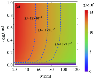
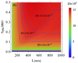
Figure 5: (Color online) The QSL time $\tau_{QSL}$ in 3D BEC reservoir as a function of the trap parameter of double-well $\sigma$ (the top subfigure) and the distance of two wells of double-well $L$ (the bottom subfigure). The blue dashed contour lines mark different given distances $\mathcal{D}$: from top to bottom, the $\mathcal{D}$ takes the value of (a) $\mathcal{D}\times 10^{5}=12,11,10$ with $L=150nm$; (b) $\mathcal{D}\times 10^{5}=15.5,15,14$ with $\sigma=45nm$. The initial-state of the impurity atom is prepared in a maximally coherent state with $x^{2}+y^{2}=1$, $z=0$. And the s-wave scattering length takes the value of $a_{B}=a_{Rb}=5.3nm$. Other parameters are the same as in Fig. 2.

Furthermore, Fig. 5 presents the influence of two spatial parameters of the double-well potential $V_{A}(\textbf{r})$ ($\sigma$ and $L$) on the DSL of the impurity atom for different regimes of the state distances in the case of the 3D BEC reservoir. Inspecting the contour lines in Fig. 5, we can find that, for a given state distance $\mathcal{D}$, the QSL time of the impurity atom $\tau_{QSL}$ in the 3D BEC reservoir increases monotonously with increasing $\sigma$, while decreases first and then oscillates with the increase of $L$. And the manipulating mechanism is more efficient in the larger $\sigma$ regime or in the small $L$ regime. That is to say, the larger $\sigma$ and smaller $L$ induce a slower DSL. These results can also be explained as a result of the effect of $\sigma$ or $L$ on the dephasing function $\Gamma(t)$, as shown in Figs. 3. And we find similar results are also applicative for the low-dimension cases. Anyway, above results provide us another way to protect the coherence of the impurity atom in its BEC reservoir.

The DSL manipulation of the impurity atom in BEC reservoir is realized by controlling the spectral density of the BEC reservoir. In order to explore a more intuitive physical insight into the effect of relevant parameters, including $a_{B}$, $D$, $\sigma$ and $L$, on the quantum dephasing process of the impurity atom, we analyze the spectral density $J(\omega)$ in details in appendix A Haikka2011 ; Hangleiter2015 ; Carole2014 . For qualitative analysis, here we mainly consider the spectral density in the low-frequency region, which plays a leading role in the long-time decoherence process. In the non-interacting BEC reservoir ($a_{B}=0$), low-energy excitations with $\omega\ll\omega_{L}$ have particle-like spectrum scaled as

$$J_{D}\left(\omega\right) \approx A_{D}\omega^{D/2}e^{-\omega/\omega_{c}},$$ (16)

where the soft cut-off frequency $\omega_{c}=\frac{1}{m_{B}\sigma^{2}}$ and three prefactors $A_{D}$ are given by Eq. (A8).

However, in the interacting BEC reservoir with $a_{B}\neq 0$, the low-energy excitations with $\omega\ll n_{D}g_{D}$ have phonon-like spectrum scaled as

$$J_{D}\left(\omega\right) \approx B_{D}\omega^{D+2}e^{-\omega^{2}/\tilde{\omega}_{c,D}^{2}},$$ (17)

where $\tilde{\omega}_{c,D}=\frac{\sqrt{2}c_{D}}{\sigma}$ with the speed of sound $c_{D}=\sqrt{\frac{n_{D}g_{D}}{m_{B}}}$, and three prefactors $B_{D}$ are given by Eq. (A10).

That is to say, for the free cases, the spectrum are sub-Ohmic, Ohmic, and super-Ohmic in $1$D, $2$D and $3$D reservoirs, respectively. However, the low-frequency spectrum for the interacting cases are always super-Ohmic, and the super-Ohmicity of the spectral density is enhanced with the increase of dimensions of the BEC reservoir. Thus, the slow down of the quantum dephasing speed induced by increasing $a_{B}$ or decreasing $D$ can be explained as a result of the change of the spectral density's Ohmicity. And another interesting phenomenon is that the cut-off frequency $\omega_{c}$ or $\tilde{\omega}_{c,D}$ can both be reduced by increasing $\sigma$, which would also suppress the dephasing of impurity induced by the high-frequency modes in the BEC reservoir. Meanwhile, the dependence of the spectrum on the distance $L$ is established through the relationship between the prefactors ($A_{D}$ or $B_{D}$) and $L$. From Eqs. (A8) and (A10), we can see that, in the small region of $L$, the effective coupling constant is proportion to $L^{2}$, which is the reason for the speedup of the quantum dephasing of the impurity with the increase of $L$.

IV Conclusions

In conclusion, we have studied the DSL of a single impurity atom immersed in a BEC reservoir with the impurity atom being in a double-well potential. We have obtained the DSL based on the quantum Fisher information formalism. We demonstrated that the DSL of the impurity atom can be manipulated by engineering the BEC reservoir and the impurity potential within experimentally realistic limits. It has been shown that the DSL can be controlled by changing key parameters such as the scattering length, the effective dimension of the BEC reservoir, and the spatial configuration of the double-well potential. In order to explore the physical mechanisms of controlling the DSL, we have analyzed the spectral density in details. It has been revealed that the physical mechanisms of controlling the DSL at root of engineering the spectral density of the BEC reservoir.

It is believed that these results of the present study may provide a direct path towards engineering quantum dephasing speed of qubits in nonlinear reservoirs, and would help to address the robustness of quantum simulators and computers in a phasing damping channel against decoherence Mukherjee2013 ; Iman2015 ; Carole2015 , which may have implications in quantum cooling and quantum thermodynamics.

Appendix A Derivation of the spectral density

In this Appendix we derive the spectral density of the impurity-BEC system. The spectral density of the impurity-BEC system is formally given by

$$J\left(\omega\right)\equiv\sum_{\mathbf{k}}\left|\xi_{\mathbf{k}}\right|^{2}\delta\left(\omega-\omega_{\mathbf{k}}\right).$$ (18)

In the continuum limit $\frac{1}{V}\sum_{\mathbf{k}}\rightarrow\frac{1}{\left(2\pi\right)^{D}}\int d\Omega_{D}\int dkk^{D-1}$ with $\Omega_{D}$ being the surface of the unit sphere in $D$ dimensions, the spectral density can be rewritten by inserting Eq. (3) into the above equation,

$$J\left(\omega\right) = \frac{\eta_{D}^{2}n_{D}}{V}\sum_{\mathbf{k}}\frac{\epsilon_{\mathbf{k}}}{\omega_{\mathbf{k}}}e^{-k^{2}\sigma^{2}/2}\sin^{2}\left(\mathbf{k}\cdot\mathbf{L}\right)\delta\left(\omega-\omega_{\mathbf{k}}\right)$$

$$= \frac{\eta_{D}^{2}n_{D}}{\left(2\pi\right)^{D}}\int dkk^{D-1}f_{D}(kL)\frac{\epsilon_{\mathbf{k}}}{\omega_{\mathbf{k}}}e^{-k^{2}\sigma^{2}/2}\delta\left(\omega-\omega_{\mathbf{k}}\right),$$

where the angular integral is defined by

$$f_{D}(kL)=\int d\Omega_{D}\sin^{2}\left(\mathbf{k}\cdot\mathbf{L}\right),$$ (20)

which can be easily calculated with the following results

$$f_{1}(kL) = \sin^{2}(kL),\hskip 14.22636ptf_{2}(kL)=\pi[1-J_{0}(2kL)],$$

$$f_{3}(kL) = 2\pi\left[1-\frac{\sin(2kL)}{2kL}\right],$$ (21)

where $J_{0}(x)$ is the first kind of Bessel function .

Let $k(\omega)$ is the root of the equation $\omega=\omega_{\mathbf{k}}$ in Eq. (2),

$$k\left(\omega\right) = \sqrt{2m_{B}\left[\sqrt{n_{D}^{2}g_{D}^{2}+\omega^{2}}-n_{D}g_{D}\right]},$$ (22)

the spectral density in Eq. (A2) becomes

$$J\left(\omega\right) = \frac{\eta_{D}^{2}n_{D}}{\left(2\pi\right)^{D}}\int d\omega_{\mathbf{k}}k^{D-1}f_{D}(kL)\frac{\epsilon_{\mathbf{k}}}{\omega_{\mathbf{k}}}$$

$$\times e^{-k^{2}\sigma^{2}/2}\left(\frac{d\omega_{\mathbf{k}}}{dk}\right)^{-1}\delta\left(\omega-\omega_{\mathbf{k}}\right)$$

$$= \frac{\eta_{D}^{2}n_{D}m_{B}}{\left(2\pi\right)^{D}}k\left(\omega\right)^{D-2}f_{D}\left[k\left(\omega\right)L\right]\frac{\epsilon_{\mathbf{k}}\left(\omega\right)e^{-k\left(\omega\right)^{2}\sigma^{2}/2}}{n_{D}g_{D}+\epsilon_{\mathbf{k}}\left(\omega\right)},$$

where the first partial derivatives of $\omega_{k}$ versus wave vector $k$ can be derived from Eq. (2), $\frac{d\omega_{\mathbf{k}}}{dk}=\frac{k\left(n_{D}g_{D}+\epsilon_{\mathbf{k}}\right)}{m_{B}\omega_{\mathbf{k}}}$.

As one can see from Eq. (2), the dispersion relation is much sensitive to the inter-atomic interaction strength $g_{D}$. In the following we consider two extreme cases. In the free boson reservoir with $g_{D}=0(a_{B}=0)$, the quasi-particle energy tends to $\omega=\frac{k^{2}}{2m_{B}}$. In the low-frequency region with $\omega\ll\omega_{L}$, the spectral density can be reduced to the simple form

$$J_{D}\left(\omega\right) \approx A_{D}\omega^{D/2}e^{-\omega/\omega_{c}},$$ (24)

where $\omega_{c}=\frac{1}{m_{B}\sigma^{2}}$ and we have introduced three prefactors

$$A_{1} = \frac{\eta_{1}^{2}n_{1}m_{B}^{3/2}L^{2}}{\sqrt{2}\pi},\hskip 14.22636ptA_{2}=\frac{\eta_{2}^{2}n_{2}m_{B}^{2}L^{2}}{2\pi},$$

$$A_{3} = \frac{\sqrt{2}\eta_{3}^{2}n_{3}m_{B}^{5/2}}{3\pi^{2}},$$ (25)

where $n_{D}$ and $\eta_{D}$ are the number density of the D-dimensional BEC and the interaction strength between impurity atoms and D-dimensional BEC with the expressions given by Eqs. (5) and (6), respectively. Making use of Eqs. (5) and (6), from Eq. (A8) we can see that the prefactors $A_{D}$ are dependent of the distance parameter between two wells $L$ and the $s$-wave scattering length $a_{AB}$ for BEC-impurity collisions.

Hence, in the non-interacting case, low-energy excitations of the BEC reservoir have particle-like spectrum given by Eq. (A7) with the soft cut-off frequency $\omega_{c}$ Haikka2011 ; Hangleiter2015 . From Eq. (A7) we can see that the Ohmicity of the BEC reservoir is determined by the dimensions of the BEC. The spectrum is sub-Ohmic, Ohmic, and super-Ohmic for 1D, 2D, and 3D BEC reservoir, respectively.

Whereas for the interacting BEC reservoir with $g_{D}\neq 0$ $(a_{B}\neq 0)$, in the low-frequency region with $\omega\ll n_{D}g_{D}$, the dispersion relation changes to the phonon-like form $\omega\approx c_{D}k$ with the speed of sound $c_{D}=\sqrt{\frac{n_{D}g_{D}}{m_{B}}}$. Thus, the spectrum can be approximately equal to

$$J_{D}\left(\omega\right) \approx B_{D}\omega^{D+2}e^{-\omega^{2}/\tilde{\omega}_{c,D}^{2}}.$$ (26)

where $\tilde{\omega}_{c,D}=\frac{\sqrt{2}c_{D}}{\sigma}$ and we have introduced three prefactors

$$B_{1} = \frac{\eta_{1}^{2}L^{2}}{4\pi g_{1}^{5/2}}\left(\frac{m_{B}}{n_{1}}\right)^{3/2},\hskip 14.22636ptB_{2}=\frac{\eta_{2}^{2}L^{2}}{8\pi g_{2}^{3}}\left(\frac{m_{B}}{n_{2}}\right)^{2},$$

$$B_{3} = \frac{\eta_{3}^{2}L^{2}}{12g_{3}^{7/2}\pi^{2}}\left(\frac{m_{B}}{n_{3}}\right)^{5/2}.$$ (27)

where $g_{D}$ is the interaction strength between inter-atomic interaction in D-dimensional BEC with the expressions given by Eq. (4). Making use of Eqs. (4)-(6), from Eq. (A10) we can see that the prefactors $B_{D}$ depends on not only the distance parameter between two wells $L$ and the $s$-wave scattering length for impurity-BEC collisions $a_{AB}$, but also the scattering length for inter-atomic collisions $a_{B}$. Therefore, in the case of the interacting BEC reservoir, low-energy excitations of the reservoir have phonon-like spectrum given by Eq. (A9). The spectral Ohmicity of the BEC reservoir is always super-Ohmic for 1D, 2D, and 3D BEC reservoir.

References

- (1) H. P. Breuer and F. Petruccione, The theory of open quantum systems (Oxford University Press, New York,2002).
- (2) A. Leggett, S. Chakravarty, A. T. Dorsey, M. P. A. Fisher, A. Garg, and W. Zwerger, Dynamics of the dissipative two-state system, Rev. Mod. Phys. 59, 1 (1987).
- (3) N. V. Prokof'ev and P. Stamp, Theory of the spin bath, Rep. Prog. Phys. 63, 669 (2000).
- (4) L. M. Kuang, H. S. Zeng, and Z. Y. Tong, Nonlinear decoherence in quantum state preparation of a trapped ion, Phys. Rev. A 60, 3815 (1999).
- (5) L. M. Kuang, X. Chen, and M. L. Ge, Influence of intrinsic decoherence on nonclassical effects in the multiphoton Jaynes-Cummings model, Phys. Rev. A 52, 1857 (1995).
- (6) L. M. Kuang, Z. Y. Tong, Z. W. Ouyang, and H. S. Zeng, Decoherence in two Bose-Einstein condensates, Phys. Rev. A 61, 013608 (1999)
- (7) J. Q. Liao, J. F. Huang, and L. M. Kuang, Quantum thermalization of two coupled two-level systems in eigenstate and bare-state representations, Phys. Rev. A 83, 052110 (2011)
- (8) J. B. Yuan, L. M. Kuang, J. Q. Liao, Amplification of quantum discord between two uncoupled qubits in a common environment by phase decoherence, J. Phys. B: At. Mol. Opt. Phys. 43, 165503 (2010).
- (9) J. Lu, L. Zhou, H. C. Fu, and L. M. Kuang, Quantum decoherence in a hybrid atom-optical system of a one-dimensional coupled-resonator waveguide and an atom, Phys. Rev. A 81, 062111 (2010).
- (10) Z. He, H. S. Zeng, Y. Li, Q. Wang, C. M. Yao, Non-Markovianity measure based on the relative entropy of coherence in an extended space, Phys. Rev. A 96, 022106 (2017).
- (11) L. Mandelstam and I. G. Tamm, The uncertainty relation between energy and time in nonrelativistic quantum mechanics. J. Phys. (USSR) 9, 249 (1945).
- (12) N. Margolus and L. B. Levitin, The maximum speed of dynamical evolution. Phys. D 120, 188-195 (1998).
- (13) V. Giovannetti, S. Lloyd, and L. Maccone, Quantum limits to dynamical evolution. Phys. Rev. A 67, 052109 (2003).
- (14) M. M. Taddei, B. M. Escher, L. Davidovich, and R. L. de Matos Filho, Quantum speed limit for physical processes. Phys. Rev. Lett. 110, 050402 (2013).
- (15) A. del Campo, I. L. Egusquiza, M. B. Plenio, and S. F. Huelga, Quantum speed limits in open system dynamics. Phys. Rev. Lett. 110, 050403 (2013).
- (16) S. Deffner and E. Lutz, Quantum speed limit for non-Markovian dynamics. Phys. Rev. Lett. 111, 010402 (2013).
- (17) S. Deffner and S. Campbell, Quantum speed limits: from Heisenberg's uncertainty principle to optimal quantum control. J. Phys. A: Math. Theor. 50, 453001 (2017).
- (18) D. P. Pires, M. Cianciaruso, L. C. Ceri, G. Adesso, and D. O. Soares-Pinto, Generalized geometric quantum speed limits. Phys. Rev. X 6, 021031 (2016).
- (19) A. D. Cimmarusti, Z. Yan, B. D. Patterson, L. P. Corcos, L. A. Orozco, and S. Deffner, Environment-Assisted Speed-up of the Field Evolution in Cavity Quantum Electrodynamics. Phys. Rev. Lett. 114, 233602 (2015).
- (20) P. J. Jones and P. Kok, Geometric derivation of the quantum speed limit. Phys. Rev. A 82, 022107(2010).
- (21) Y.-J. Zhang, W. Han, Y.-J. Xia, J.-P. Cao, and H. Fan, Quantum speed limit for arbitrary initial states. Sci. Rep. 4, 4890 (2014).
- (22) Z. Sun, J. Liu, J. Ma, and X. Wang, Quantum speed limits in open systems: non-Markovian dynamics without rotating-wave approximation. Sci. Rep. 5, 8444 (2015).
- (23) N. Mirkin, F. Toscano, and D. A. Wisniacki, Quantum-speed-limit bounds in an open quantum evolution. Phys. Rev. A 94, 052125 (2016).
- (24) Z. Y. Xu, Detecting quantum speedup in closed and open systems. New J. Phys. 18, 073005 (2016).
- (25) X. Meng, C. Wu, and H. Guo, Minimal evolution time and quantum speed limit of non-Markovian open systems. Sci. Rep. 5, 16357 (2015).
- (26) Y. J. Song, L. M. Kuang, and Q. S. Tan, Quantum speedup of uncoupled multiqubit open system via dynamical decoupling pulses. Quantum Infor. Process. 15, 2325 (2016).
- (27) Y. J. Song, Q. S. Tan, and L. M. Kuang, Control quantum evolution speed of a single dephasing qubit for arbitrary initial states via periodic dynamical decoupling pulses. Sci. Rep. 7, 43654 (2017).
- (28) S. Deffner, Geometric quantum speed limits: A case for Wigner phase space. New J. Phys. 19, 103018 (2017).
- (29) F. Campaioli, F. A. Pollock, F. C. Binder, and K. Modi, Tightening Quantum Speed Limits for Almost All States. Phys. Rev. Lett. 120, 060409 (2018).
- (30) M. Mo, J. Wang, and Y. Wu, Quantum speedup via engineering multiple environments. Ann. Phys. 5, 1600221 (2017).
- (31) J. Lee, C. Arenz, H. Rabitz, and B. Russell, Dependence of the quantum speed limit on system size and control complexity. New J. Phys. 20, 063002 (2018).
- (32) I. Bloch, J. Dalibard, and W. Zwerger, Many-body physics with ultracold gases. Rev. Mod. Phys. 80, 885 (2008).
- (33) M. A. Cirone, G. De Chiara, G. M. Palma, and A. Recati, Collective decoherence of cold atoms coupled to a BoseEinstein condensate. New J. Phys. 11, 103055 (2009).
- (34) P. Haikka, S. McEndoo, G. De Chiara, G. M. Palma, and S. Maniscalco, Quantifying, characterizing, and controlling information flow in ultracold atomic gases. Phys. Rev. A 84, 031602 (2011).
- (35) A. Klein, M. Bruderer, S. R. Clark, and D. Jaksch, Dynamics, dephasing and clustering of impurity atoms in BoseEinstein condensates. New J. Phys. 9, 411 (2007).
- (36) J. B. Yuan, H. J. Xing, L. M. Kuang, and S. Yi, Quantum non-Markovian reservoirs of atomic condensates engineered via dipolar interactions. Phys. Rev. A 95, 033610 (2017).
- (37) E. M. Lifshitz and L. P. Pitaevskii, Statistical Physics, Part 2 (Pergamon Press, Oxford, 1980).
- (38) P. hberg, E. L. Surkov, I. Tittonen, S. Stenholm, M. Wilkens, and G. V. Shlyapnikov, Low-energy elementary excitations of a trapped Bose-condensed gas. Phys. Rev. A 56, R3346 (1997).
- (39) L. Zhou, J. Lu, D. L. Zhou, and C. P. Sun, Quantum theory for spatial motion of polaritons in inhomogeneous fields. Phys. Rev. A 77, 023816 (2008).
- (40) Y. Guo, L. Zhou, L. M. Kuang, and C. P. Sun, Magneto-optical Stern-Gerlach effect in an atomic ensemble. Phys. Rev. A 78, 013833 (2008).
- (41) L. P. Pitaevskii and S. Stringari, Bose-Einstein condensation (Clarendon Press, Oxford, 2003).
- (42) P. Naidon, E. Tiesinga, W. F. Mitchell, and P. S. Julienne, Effective-range description of a Bose gas under strong one- or two-dimensional confinement. New J. Phys. 9, 19 (2007).
- (43) D. Hangleiter, M. T. Mitchison, T. H. Johnson, M. Bruderer, M. B. Plenio, and D. Jaksch, Nondestructive selective probing of phononic excitations in a cold Bose gas using impurities. Phys. Rev. A 91, 013611 (2015).
- (44) P. Naidon and P. S. Julienne, Optical Feshbach resonances of alkaline-earth-metal atoms in a one- or two-dimensional optical lattice. Phys. Rev. A 74, 062713 (2006).
- (45) J. Catani, G. Lamporesi, D. Naik, M. Gring, M. Inguscio, F. Minardi, A. Kantian, and T. Giamarchi, Quantum dynamics of impurities in a one-dimensional Bose gas. Phys. Rev. A 85, 023623 (2012).
- (46) S. Blanes, F. Casas, J. A. Oteo, and J. Ros, The Magnus expansion and some of its applications. Phys. Rep. 470, 151 (2009).
- (47) D. Jaksch, C. Bruder, J. I. Cirac, C. W. Gardiner, and P. Zoller, Cold bosonic atoms in optical lattices. Phys. Rev. Lett. 81, 3108 (1998).
- (48) C. W. Helstrom, Quantum detection and estimation theory (Academic, New York, 1976).
- (49) C. Addis, G. Brebner, P. Haikka, and S. Maniscalco, Coherence trapping and information backflow in dephasing qubits. Phys. Rev. A 89, 024101 (2014).
- (50) V. Mukherjee, A. Carlini, A. Mari, T. Caneva, S. Montangero, T. Calarco, R. Fazio, and V. Giovannetti, Speeding up and slowing down the relaxation of a qubit by optimal control. Phys. Rev. A 88, 062326 (2013).
- (51) I. Marvian and D. A. Lidar, Quantum speed limits for leakage and decoherence. Phys. Rev. Lett. 115, 210402 (2015).
- (52) C. Addis, F. Ciccarello, M. Cascio, G. Palma, and S. Maniscalco, Dynamical decoupling efficiency versus quantum non-Markovianity. New J. Phys. 17, 123004 (2015).