A HYBRID NEURAL NETWORK FRAMEWORK AND APPLICATION TO RADAR AUTOMATIC TARGET RECOGNITION

Abstract

Deep neural networks (DNNs) have found applications in diverse signal processing (SP) problems. Most efforts either directly adopt the DNN as a black-box approach to perform certain SP tasks without taking into account of any known properties of the signal models, or insert a pre-defined SP operator into a DNN as an add-on data processing stage. This paper presents a novel hybrid-NN framework in which one or more SP layers are inserted into the DNN architecture in a coherent manner to enhance the network capability and efficiency in feature extraction. These SP layers are properly designed to make good use of the available models and properties of the data. The network training algorithm of hybrid-NN is designed to actively involve the SP layers in the learning goal, by simultaneously optimizing both the weights of the DNN and the unknown tuning parameters of the SP operators. The proposed hybrid-NN is tested on a radar automatic target recognition (ATR) problem. It achieves high validation accuracy of 96% with 5,000 training images in radar ATR. Compared with ordinary DNN, hybrid-NN can markedly reduce the required amount of training data and improve the learning performance.

Index Terms—  Hybrid neural network, deep learning, signal processing, radar imaging, automatic target recognition

1 Introduction

During the recent decade, deep learning technology, particularly deep neural network (DNN), has gained tremendous popularity in various fields including signal processing (SP) [1, 2, 3, 4]. As a data-driven framework, DNN treats the learning problem as a “black-box” that extracts useful features directly from data. With sufficient training, DNN does not rely on any special structure or property of the processed data, making it universally applicable to diverse problem models. As such, DNN can help to expand the functionality of SP to handle problems that cannot be well-modeled, such as automatic target recognition (ATR) in radar [5, 6, 7].

However, improved universality may lead to worsened specialty, that is, a universally good solution is often non-optimal in terms of either accuracy or efficiency. Specializing to the SP field, there are abundant highly-structured or man-made signals with known properties, such as low-rankness or sparsity. DNN, as a data-driven approach which is blind to specialized signal structures, is obviously not as efficient in processing and extracting useful information from those signals with known models and properties. In contrast, traditional SP methods are typically crafted to gainfully utilize such prior knowledge. It is desired to combine SP and DNN judiciously so as to benefit from both sides.

Most efforts on combining SP with DNN fall under two categories. One is to treat a DNN as a module and insert it into the conventional SP framework to handle some subtasks [8]. Conversely, the other is to attach some SP modules to the DNN framework, either before/after the network as a pre-/post-processing stage, or inside the network to perform some specific data processing [9, 10]. Both approaches can be successful in demonstrating the power of DNN in learning features from complex models and validating the efficiency of SP in dealing with structured data. Common to these approaches, the adopted SP operators are pre-defined as “hyper-parameters” of the learning problem, in the sense that all design parameters of the SP operators have to be known a priori and fixed during training. Unfortunately, adopting pre-defined SP operators encounters two major challenges. First, it can be difficult to pre-define some SP operators because of the difficulty in setting its design parameters since they may be unknown or cannot be estimated accurately. Second, in the real world, the properties and structural models of the processed data can be partially known only, in the form of a “gray-box”. Hence, we wish to not only embed some appropriate SP modules into the DNN to effectively utilize those partially available data properties, but also allow some tuning “parameters” of the SP modules to be updated and optimized during training given a specific learning objective.

This paper develops a holistic approach of combining SP operators and DNN that overcomes the aforementioned challenges. A hybrid neural network (hybrid-NN) is proposed, in which one or more properly-selected SP operators are inserted into the DNN architecture as embedded layers, and some key design parameters of each SP operator are treated as unknowns and updated during network training from data. To perform efficient training for the hybrid-NN, the (sub-)gradients of SP operators are utilized to compute the training error of each SP layer, which is then incorporated into the back-propagation method for iterative network training. The proposed training algorithm can can simultaneously train the weights of the DNN and optimize the unknown tuning parameters of the SP operators from the labeled data. aThe hybrid-NN offers a viable framework to take advantages of the strengths from both ordinary DNN and SP: the SP layers utilize the partially known models of the data to improve the sample efficiency in feature extraction, and the DNN architecture offers universality in learning the remaining unknown models and features from data. Simulation results on a radar ATR problem corroborate that the hybrid-NN offers enhanced capability in feature extraction, and can markedly reduce the amount of training data needed for DNN learning.

2 Deep Neural Network

Deep neural network [1] is a highly structured framework. A typical DNN architecture is shown in the left part of Figure 1, which is composed of many nonlinear processing stages, denoted as “layers”, where each layer’s output feeds to its immediate next layer as the input. For a DNN with $I$ layers, the relationship between input $\mathbf{x}^{i-1}$ and output $\mathbf{x}^{i}$ of a specific layer $i,1\leq i\leq I,$ can be described as:

$$\mathbf{x}^{i}=f^{i}(\mathbf{W}^{i},\mathbf{b}^{i};\mathbf{x}^{i-1})=f^{i}(\mathbf{W}^{i}\mathbf{x}^{i-1}+\mathbf{b}^{i}),$$ (1)

where $f^{i}(\cdot)$ is the activation function, $\mathbf{W}^{i}$ denotes the weights and $\mathbf{b}^{i}$ denotes the bias of the $i$-th layer. Usually $f^{i}(\cdot)$ is a non-linear function, e.g. sigmoid, tanh or ReLU [1, 11].

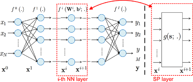
Fig. 1: Diagram of (Hybrid) Neural Network

The entire network can be viewed as a cascade of function series $f^{i}(\cdot),i=1,\dots,I,$ as:

$$\begin{split}\mathbf{y}&=f^{I}(\mathbf{W}^{I},\mathbf{b}^{I};f^{I-1}(\mathbf{W}^{I-1},\mathbf{b}^{I-1};\dots f^{1}(\mathbf{W}^{1},\mathbf{b}^{1};\mathbf{x}^{0})))\\ &=f(\mathbf{W},\mathbf{b};\mathbf{x}^{0}),\end{split}\vspace{-.5em}$$ (2)

where $\mathbf{x}^{0}$ is the input and $\mathbf{y}$ is the output of the entire network. The multi-layered DNN structure in (2) is attractive for its good universal function approximating ability [12], which means that with a sufficient amount of training data, it is possible to use (2) to fit very complex problems via updating the parameters $(\mathbf{W};\mathbf{b})$.

The training stage usually adopts the back-propagation (BP) method [1, 13]. In each iteration of the BP method, the error of each layer is propagated backwards from the output layer to the input layer, and the update value of parameters in each layer is calculated simultaneously with the error propagation by calculating the gradient as:

$$\Delta\mathbf{W}^{i}=-\lambda\left(\frac{\partial f^{i}}{\partial\mathbf{W}^{i}}\right)\boldsymbol{\delta}^{i},\quad\boldsymbol{\delta}^{i-1}=\left(\frac{\partial f^{i}}{\partial\mathbf{x}^{i-1}}\right)\boldsymbol{\delta}^{i},$$ (3)

where $\Delta\mathbf{W}^{i}$ is the parameter update value of the $i$-th layer, $\boldsymbol{\delta}^{i}$ is the output error of the $i$-th layer (which is propagated from the $(i+1)$-th layer), $\lambda$ is the learning rate and $\boldsymbol{\delta}^{i-1}$ is the error propagated back to the $(i-1)$-th layer.

3 Hybrid Neural Network

3.1 Hybrid Neural Network Design

In deep learning applications, the multi-layered framework in (2) provides excellent approximation ability in a wide range of problems. However, in some specific problems the layer model in (1) might not have the best approximation ability. This fact inspires us to design a specific signal processing (SP) layer which is optimized for some special input data, and replace one (or some) layer(s) in the ordinary DNN to achieve a better feature extraction ability in some problems. The SP layer is designed following specific conventional SP operator based on some signal property that we want to utilize. Meanwhile, some parameters are not or cannot be pre-defined in the SP layer, but to be fine tuned in the training stage.

Suppose that $\mathbf{x}^{i-1}$, the $(i-1)$-th layer’s output of an ordinary DNN, can be effectively processed by a SP operator $p$ with parameters $\mathbf{s}$, but $\mathbf{s}$ is either unknown or needed to be fine tuned. Denoting the output of this SP method as $\tilde{\mathbf{x}}^{i}$, the relationship between $\mathbf{x}^{i-1}$ and $\tilde{\mathbf{x}}^{i}$ can be described as a mapping:

$$\tilde{\mathbf{x}}^{i}=p(\mathbf{s};\mathbf{x}^{i-1}).$$ (4)

Incorporating with an activation function $f^{i}(\cdot)$ (which can be chosen as any conventional DNN activation function), we can construct a network layer $g(\cdot)$ as:

$$\mathbf{x}^{i}=g(\mathbf{s};\mathbf{x}^{i-1})=f^{i}\left(p(\mathbf{s};\mathbf{x}^{i-1})\right).$$ (5)

We call (5) as the SP layer. We can insert this SP layer into an ordinary DNN by replacing one of its conventional layers. A DNN with its $i$-th layer replaced by (5) is expressed as:

$$\begin{split}\mathbf{y}&=f^{I}(\mathbf{W}^{I},\mathbf{b}^{I};\dots g(\mathbf{s};\dots f^{1}(\mathbf{W}^{1},\mathbf{b}^{1};\mathbf{x}^{0})))\\ &=f^{\prime}(\mathbf{W},\mathbf{b},\mathbf{s};\mathbf{x}^{0}),\end{split}$$ (6)

which is shown in the right part of Figure 1. This modified DNN is named as hybrid neural network, or hybrid-NN in short.

The choice of mapping $p(\cdot)$ varies in applications in order to achieve the best feature extraction ability. For example, if $\mathbf{x}^{i-1}$ happens to be a BPSK signal (although we do not know its accurate parameters), the SP operator $p(\cdot)$ at the $i$-th layer can be chosen as a BPSK demodulator:

$$p(\omega,\eta;\mathbf{x}^{i-1})=\mathrm{conv}(F(\eta),\mathbf{r}(\omega)^{\mathrm{T}}\mathbf{x}^{i-1}),$$ (7)

where $\mathrm{conv}(\cdot)$ is the convolution operator, $F(\eta)$ is a low-pass filter parameterized by $\eta$ and $\mathbf{r}(\omega)$ is the reference signal with carrier frequency $\omega$. Key to this SP layer is that we adopt the convolution operator to make use of the model structure of an optimal BPSK demodulator, and at the same time allow the key parameters $\mathbf{s}:=(\eta,\omega)$ to be unknown a priori, such that they can be learned during training.

3.2 Hybrid Neural Network Training Algorithm

As a novel DNN architecture, we develop the training algorithm of hybrid-NN in this subsection. Since the overall architecture of hybrid-NN is still a layer-wise structure, we can adopt the conventional BP method [1, 13] to train it. The key is to deal with the SP layer(s): how to update the parameters $\mathbf{s}$ in SP layer, and how to back-propagate the error to its neighboring layer.

Assume that the partial derivatives of the SP operator in (5) exist. Given the $i$-th layer is SP and the output error of this layer is:

$$\boldsymbol{\delta}^{i}=\boldsymbol{\delta}^{i+1}f^{i\prime}\left(p(\mathbf{s};\mathbf{x}^{i-1})\right),$$ (8)

where $\boldsymbol{\delta}^{i+1}$ is the error from $(i+1)$-th layer and $f^{i\prime}$ is the derivative of the activation function. Then, the update value of $\mathbf{s}$ and the output error back-propagated to previous layer can be calculated by gradient descent as:

$$\Delta\mathbf{s}=-\lambda\left(\frac{\partial p}{\partial\mathbf{s}}\right)\boldsymbol{\delta}^{i},\quad\boldsymbol{\delta}^{i-1}=\left(\frac{\partial p}{\partial\mathbf{x}^{i-1}}\right)\boldsymbol{\delta}^{i},$$ (9)

where $\lambda$ is the learning rate.

Remark 1: Complex values. Complex values are inevitable in hybrid-NN because complex-valued signals are common in signal processing problems. One straightforward training approach is to calculate the gradient in (8) and (9) using Wirtinger calculus [14].

Remark 2: Subgradient. In case the SP operator in (5) is not differentiable, we can still use (8) and (9) by replacing the derivatives by subderivatives.

Remark 3: Size of the training dataset. Compared with the ordinary DNN, a hybrid-NN only works for specific problems that the SP method $p(\cdot)$ is suitable for. As the reward, SP layer is expected to have better feature extraction ability, which in turn reduces the number of training iterations. Furthermore, usually the size of $\mathbf{s}$ is much smaller than the size of $(\mathbf{W}^{i};\mathbf{b}^{i})$ in an ordinary DNN layer, which means the number of unknown parameters can be reduced and we can use less data to train it.

3.3 Discussions

3.3.1 SP Layer Placement

In general, the location index $i$ of the SP layer can be any value between $1$ and $I$ which is the number layers in the neural network. But the SP layer usually works effectively for structured or modeled input data. Currently, the interpretation of data inside hidden layers of an ordinary DNN (which means $2\leq i\leq I-1$) is still a huge challenge, making us difficult to find a suitable SP operator. The most well-understood data of DNN are its inputs and outputs, i.e. $\mathbf{x}^{0}$ and $\mathbf{y}$, which means that at current stage we prefer to put the SP layer at the beginning or the end of a hybrid-NN.

3.3.2 Difference From Pre-/Post-processing

Compared with existing work of combing SP and DNN such as [9, 10], the SP operator in in the hybrid-NN is no longer a hyper-parameter that is determined before training. In fact, it can be any (sub-)differentiable SP operator with unknown $\mathbf{s}$. We leave $\mathbf{s}$ as a parameter of hybrid-NN to learn it from data, which provides us with enhanced design flexibility compared with existing work.

4 Application of Hybrid-NN in Radar Automatic Target Recognition

In order to demonstrate the feasibility of hybrid-NN, we show an example in radar automatic target recognition (ATR). ATR refers to identifying and classifying the targets automatically from the received data, in contrast to the traditional human-aided target recognition. State-of-the-art DNN-based radar ATR techniques use a two-stage approach, which firstly generates the radar image from the raw radar signal via signal processing algorithms [15], and then perform automatic classification using DNN methods [5, 6, 7], as described in Figure 2(a). Unfortunately, such SP-based pre-processing is not always applicable in practice, because some radar parameters are either unavailable or unreliable which makes the traditional radar signal processing impossible.

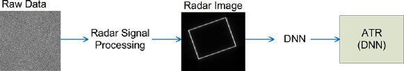
(a) Conventional ATR Using DNN

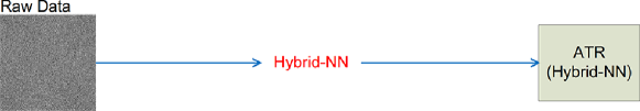
(b) Proposed ATR Using Hybrid-NN

Fig. 2: Radar ATR Frameworks

In this paper, we suggest a novel ATR framework as shown in Figure 2(b), which directly performs automatic classification from the raw radar signals using hybrid-NN, bypassing the radar signal processing stage. The SP and DNN are coherently combined, which is particularly attractive for real-time ATR, as well as in situations where some radar parameters need to be learned or tuned.

4.1 Radar Model

Consider a simple radar signal model, where a radar transmits chirp waveforms to a point target which is uniformly moving in a straight line with backscattering coefficient $\sigma$. The received baseband echo is given in [15]:

$$s(\tau,t)\approx\sigma\exp(j\pi K_{r}(\tau-\tau_{0})^{2})\exp(-j\pi K_{a}(t-t_{0})^{2}),$$ (10)

where $K_{r}$ is the range frequency modulation rate, $\tau$ is the range time, $K_{a}$ is the azimuth frequency modulation rate, $t$ is the azimuth time, $\tau_{0}$ is the range time delay and $t_{0}$ is the azimuth time that the target passes through the nearest point of the target moving trajectory with respect to the radar.

The raw radar data is stored as a 2-D data matrix $\mathbf{S}$ whose entries are digital samples of $s(\tau,t)$ along $\tau$ and $t$, with range sampling rate $F_{\mathrm{sr}}$ and pulse repetition frequency (azimuth sampling rate) $\mathrm{PRF}$. These sampling rates are selected by user.

4.2 Architecture of Hybrid-NN for Radar ATR

Radar ATR is basically a classification problem. Given labeled training data, it is straightforward to train a universal convolutional neural network (CNN) for target classification, in the absence of any knowledge of the signal model in (10). Alternatively, our hybrid-NN approach is make use of (10) for improved efficiency in training and learning. Our key step is to design a suitable radar signal processing layer, and insert this layer into a proper location of an ordinary CNN, proposing a hybrid-NN for radar ATR from raw data.

Conventional SP algorithms for radar are based on matched filtering (MF). The corresponding matched filter for (10) is:

$$m(\tau,t)=\exp\left(-j\pi\hat{K}_{r}\tau^{2}\right)\exp\left(j\pi\hat{K}_{a}t^{2}\right).$$ (11)

Ideally, the MF parameters $(\hat{K_{a}}，\hat{K_{r}})$ are determined by $K_{a}$ and $K_{r}$. But in real applications, $K_{a}$ and $K_{r}$ are either unknown (e.g. passive radar) or inaccurate due to platform and system errors, hence $(\hat{K_{a}}，\hat{K_{r}})$ are needed to be trained.

Accordingly, we design a MF layer as:

$$\begin{split}g(\hat{K_{a}},\hat{K_{r}};\mathbf{S})&=f\left(\mathrm{conv}\big{\{}\mathbf{M}(\hat{K_{a}},\hat{K_{r}}),\mathbf{S}\big{\}}\right)\\ &=\left|\mathrm{conv}\big{\{}\mathbf{M}(\hat{K_{a}},\hat{K_{r}}),\mathbf{S}\big{\}}\right|,\end{split}$$ (12)

where the activation function $f(\cdot)$ is chosen as the absolute value function $|\cdot|$, $\mathbf{S}$ is the radar raw data and $\mathbf{M}(\hat{K_{a}},\hat{K_{r}})$ is the matched filter defined as (11). The $(m,n)$-th element of $\mathbf{M}$ is:

$$\left[\mathbf{M}(\hat{K_{a}},\hat{K_{r}})\right]_{mn}=e^{-j\pi\hat{K_{r}}m^{\prime 2}}e^{j\pi\hat{K}_{a}n^{\prime 2}},$$ (13)

where $m^{\prime}=\frac{m}{F_{\mathrm{sr}}}$ and $n^{\prime}=\frac{n}{\mathrm{PRF}}$.

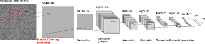
Fig. 3: Architecture of Hybrid-NN for Radar ATR

The MF layer is used as the first layer of the network and followed by an ordinary CNN. The concept is intuitive: MF layer is capable of utilizing the known properties of the radar data in terms of radar waveform structure, and then the extracted information by MF is fed into an ordinary CNN to do classification. During the training stage, the SP-layer parameters $\mathbf{s}:=(\hat{K}_{a},\hat{K}_{r})$ will be updated automatically through the BP algorithm presented in Section 3.2. The configuration of the hybrid-NN is shown in Figure 6. The network is composed of one matched filtering layer, three convolutional layers ($5\times 5\times 8,5\times 5\times 8$ and $4\times 4\times 8$) and one fully connected layer ($64$). The size of matched filter is $64\times 64$. For an ordinary convolutional layer, a $64\times 64$ kernel has $4,096$ parameters to learn, but for a matched filtering layer we only have two parameters $\hat{K_{a}}$ and $\hat{K_{r}}$ to determine. This provides us a great reduction on the amount of training data. The network is trained using the algorithm given in Subsection 3.2.

5 Simulations

5.1 Data Generation

Simulation data is generated to train and validate the performance of the proposed hybrid-NN for radar ATR. The training set includes three types of targets: circles, squares and triangles which are generated with random magnitudes, random deformations and random noises, as shown in Figure 4. The radar parameters are given in Table 1. Also note that radar raw data size are usually very large, here set as $512\times 512$. Such a large input size incurs tremendous computational load to the training stage of ordinary DNN.

(a) Raw Data

(b) Circle

(c) Square

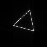
(d) Triangle

Fig. 4: Samples Data for Radar ATR

Table 1: Simulation Parameters

Carrier Frequency	5 GHz
Range Sampling Rate	600 MHz
Pulse Duration	$10\mathrm{\mu s}$
Range Bandwidth	500 MHz
Range Distance	5,000 m
Target Speed	100 m/s
PRF	1,000 Hz

5.2 Numerical Results

As a benchmark, an ordinary complex-valued DNN (which is in fact a CNN here) is adopted with similar architecture as the described hybrid-NN but only switches its first layer to a convolutional layer.

First, the training performance of hybrid-NN compared with conventional DNN are shown in Figure 5. A training set with 5,000 images is used, with each $\mathrm{mini\_batch}$ of 50 images and trained for 5 epochs. This is a very small training set, especially for the large input size. The proposed hybrid-NN shows great advantage on the training performance. It can be seen that during the 4th epoch, the hybrid-NN has already converged to a good optimum whereas the ordinary DNN cannot converge yet. Finally, hybrid-NN ends with 98% training accuracy, compared with 64% of the ordinary DNN. In order to determine the data requirement of the ordinary DNN, the dataset size is further increased to 25,000 images, and the network finally converged with 82% accuracy as shown in Figure 6. This simulation verifies the benefits of hybrid-NN in the training stage, including fast convergence and small training dataset size.

Second, the accuracy of trained hybrid-NN on the validation data with different noise levels is also tested in Figure 7. As the SNR is changed from -10dB to 40dB, the validation accuracy starts with 85% at -10dB and rapidly grows to 96% after 0dB. This result shows the robustness of proposed hybrid-NN and very high validation accuracy on the test data in the validation stage.

6 Conclusion

We introduce a novel hybrid-NN framework, which inject the DNN with a SP layer that is specifically designed for particular signal models. A network training algorithm is presented to simultaneously update both the network weights and the design parameters of the SP layer during training. The proposed hybrid-NN framework is tested on a radar ATR application. Compared with ordinary DNN, the proposed hybrid-NN dramatically reduces the required amount of training data and improves the training efficiency with high validation accuracy.

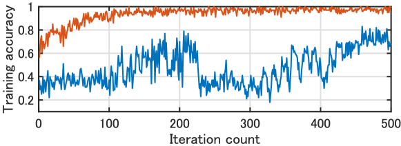
Fig. 5: Training Accuracy of Hybrid-NN and ordinary DNN with 5,000 images.

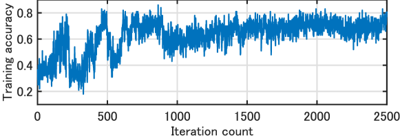
Fig. 6: Training Accuracy of ordinary DNN with 25,000 images

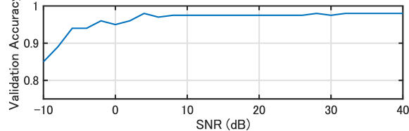
Fig. 7: Validation Accuracy with Different SNR

References

- [1] Yann LeCun, Yoshua Bengio, and Geoffrey Hinton, “Deep learning,” nature, vol. 521, no. 7553, pp. 436, 2015.
- [2] Li Deng, Dong Yu, et al., “Deep learning: methods and applications,” Foundations and Trends in Signal Processing, vol. 7, no. 3–4, pp. 197–387, 2014.
- [3] A Cochocki and Rolf Unbehauen, Neural networks for optimization and signal processing, John Wiley & Sons, Inc., 1993.
- [4] Dong Yu and Li Deng, “Deep learning and its applications to signal and information processing,” IEEE Signal Processing Magazine, vol. 28, no. 1, pp. 145–154, 2011.
- [5] David AE Morgan, “Deep convolutional neural networks for ATR from SAR imagery,” in Algorithms for Synthetic Aperture Radar Imagery XXII. International Society for Optics and Photonics, 2015, vol. 9475, p. 94750F.
- [6] Sizhe Chen, Haipeng Wang, Feng Xu, and Ya-Qiu Jin, “Target classification using the deep convolutional networks for SAR images,” IEEE Transactions on Geoscience and Remote Sensing, vol. 54, no. 8, pp. 4806–4817, 2016.
- [7] Michael Wilmanski, Chris Kreucher, and Alfred Hero, “Complex input convolutional neural networks for wide angle SAR ATR,” in 2016 IEEE Global Conference on Signal and Information Processing (GlobalSIP). IEEE, 2016, pp. 1037–1041.
- [8] Christopher A Metzler, Philip Schniter, Ashok Veeraraghavan, and Richard G Baraniuk, “prDeep: Robust phase retrieval with flexible deep neural networks,” arXiv preprint arXiv:1803.00212, 2018.
- [9] Tsung-Han Chan, Kui Jia, Shenghua Gao, Jiwen Lu, Zinan Zeng, and Yi Ma, “Pcanet: A simple deep learning baseline for image classification?,” IEEE Transactions on Image Processing, vol. 24, no. 12, pp. 5017–5032, 2015.
- [10] Brandon Amos and J Zico Kolter, “Optnet: Differentiable optimization as a layer in neural networks,” in International Conference on Machine Learning, 2017, pp. 136–145.
- [11] Xavier Glorot, Antoine Bordes, and Yoshua Bengio, “Deep sparse rectifier neural networks,” in Proceedings of the Fourteenth International Conference on Artificial Intelligence and Statistics, 2011, pp. 315–323.
- [12] Balázs Csanád Csáji, “Approximation with artificial neural networks,” Faculty of Sciences, Etvs Lornd University, Hungary, vol. 24, pp. 48, 2001.
- [13] David E Rumelhart, Geoffrey E Hinton, and Ronald J Williams, “Learning representations by back-propagating errors,” nature, vol. 323, no. 6088, pp. 533, 1986.
- [14] Md Faijul Amin, Muhammad Ilias Amin, Ahmed Yarub H Al-Nuaimi, and Kazuyuki Murase, “Wirtinger calculus based gradient descent and levenberg-marquardt learning algorithms in complex-valued neural networks,” in International Conference on Neural Information Processing. Springer, 2011, pp. 550–559.
- [15] Ian G Cumming and Frank H Wong, Digital processing of synthetic aperture radar data: Algorithms And Implementation, Artech house, 2005.