Decay of turbulence in a liquid metal duct flow with transverse magnetic field

Abstract

Decay of honeycomb-generated turbulence in a duct with a static transverse magnetic field is studied via direct numerical simulations. The simulations follow the revealing experimental study of Sukoriansky et al. (1986), in particular the paradoxical observation of high-amplitude velocity fluctuations, which exist in the downstream portion of the flow when the strong transverse magnetic field is imposed in the entire duct including the honeycomb exit, but not in other configurations. It is shown that the fluctuations are caused by the large-scale quasi-two-dimensional structures forming in the flow at the initial stages of the decay and surviving the magnetic suppression. Statistical turbulence properties, such as the energy decay curves, two-point correlations and typical length scales are computed. The study demonstrates that turbulence decay in the presence of a magnetic field is a complex phenomenon critically depending on the state of the flow at the moment the field is introduced.

1 Introduction

This paper addresses decay of turbulence in an electrically conducting fluid in the presence of an imposed static magnetic field. The parameters typical for technological and laboratory flows of liquid metals are considered, so the quasi-static (also called non-inductive) approximation, according to which the magnetohydrodynamic flow-field interaction is reduced to the effect of the imposed field on a flow, is adopted (see, e.g., Davidson, 2016, for the derivation and a discussion of validity of the approximation).

In any three-dimensional flow of an electrically conducting fluid, an imposed magnetic field suppresses turbulent fluctuations via the Joule dissipation of induced electric currents. Unlike its viscous counterpart, the Joule dissipation is active irrespective of the length scale, and anisotropic in the sense that its rate is proportional to the square of the gradient of velocity along the magnetic field lines. As described by Moffatt (1967), this transforms an initially isotropic flow into a flow with reduced or even zero velocity gradients along the magnetic field lines. In flows with walls, the picture is more complex due to the effect of walls on the velocity and electric currents. In particular, in the case of an MHD duct, the mean flow is changed by the Lorentz force, and special boundary layers appear (see, e.g., Branover, 1978; Müller & Bühler, 2001). The principal features of the transformation of turbulence still remain (1) suppression of fluctuations, so the MHD flows are found in a laminar or transitional state at much higher Reynolds numbers than their hydrodynamic counterparts (see, e.g., Zikanov et al., 2014a, for a review), and (2) dimensional anisotropy with weaker velocity gradients along the field lines than across them (see, e.g., Moffatt, 1967; Davidson, 1997; Zikanov & Thess, 1998; Vorobev et al., 2005; Krasnov et al., 2008; Reddy & Verma, 2014; Verma, 2017). The anisotropy may reach the asymptotic state of flow’s quasi- (i.e. to the degree allowed by the boundary conditions) two-dimensionality if the magnetic field is sufficiently strong to suppress three-dimensional instabilities inherently present in such a flow (Thess & Zikanov, 2007).

The term anisotropy is used in this paper with the meaning commonly employed in the research of MHD turbulence (see, e.g., Zikanov & Thess, 1998; Vorobev et al., 2005; Knaepen & Moin, 2004; Knaepen et al., 2004)–as the persistent inequality of the typical length scales of the flow structures in the directions along and across the magnetic field. The anisotropy of the Reynolds stress tensor (the inequality of velocity components) is, as discussed, e.g., by Burattini et al. (2010); Favier et al. (2010, 2011); Verma & Reddy (2015) not caused directly by the magnetic field and strongly affected by the presence of walls and other features of a particular flow, as well as the typical length scale at which the velocity is considered.

It must be stressed that while the picture outlined above is generally correct for any transformation of conventional three-dimensional turbulence, MHD flows exhibit complex and often counterintuitive behavior. Good examples are the flow regimes with spatially localized or intermittent turbulence reported by Zikanov et al. (2014a); Boeck et al. (2008); Krasnov et al. (2013); Brethouwer et al. (2012); Krasnov et al. (2012); Zikanov et al. (2014b), and the experimental demonstration by Pothérat & Klein (2014, 2017) that under certain circumstances the magnetic field can, in fact, enhance turbulence.

A starting point of the modern understanding of the decay of quasi-static MHD turbulence in a uniform field is the theoretical analysis of Moffatt (1967). A linearized model based on the assumption of a very strong magnetic field acting on an initially isotropic flow was used and the concept of the magnetically induced anisotropy was established, which largely formed the basis of the future work. The other results of Moffatt (1967), such as the power law of the energy decay $\sim t^{-1/2}$ and the asymptotically reached energy partition such that the energy of the field-parallel velocity component becomes two times larger than in the transverse components, have later been found to be non-universal (see, e.g., discussion in Burattini et al., 2010). Verma (2017) also critically reviews some of Moffatt’s ideas.

A theoretical model of decaying homogeneous turbulence was developed by Davidson (1997) (see also Davidson, 2016). Estimates of the rates of viscous and Joule dissipation in terms of the integral length scales along and across the magnetic field have led to a simple model of the decay. It shows that power-law scaling of energy with time is only possible when one dissipation mechanism is much stronger than the other. In general, the decay rate varies with the flow’s anisotropy in the course of the process.

Numerical simulations of homogeneous decaying MHD turbulence in the framework of the periodic box model were performed by Schumann (1976); Knaepen & Moin (2004); Burattini et al. (2010); Favier et al. (2011). The results of simulations of Schumann (1976) and, to a lesser degree, of Favier et al. (2011) were limited to the behavior at small Reynolds numbers due to the DNS accuracy requirements and the rapid magnetic suppression of turbulence. The limitations were avoided by Knaepen & Moin (2004) and Burattini et al. (2010) via the use of the dynamic Smagorinsky LES model, which had been demonstrated to be reliably accurate for the MHD quasi-static turbulence by Knaepen & Moin (2004); Vorobev et al. (2005); Vorobev & Zikanov (2007). It was confirmed by Burattini et al. (2010) that the linear model of Moffatt (1967) is only valid for very strong magnetic suppression and during short (less than one turnover time) transformation of the flow. Otherwise, the evolution is complex and strongly influenced by the large-scale anisotropic structures forming in the flow during the initial decay period. This implies inevitable influence of the boundaries and, in general, lack of universality of the decay behavior.

Experimental reproduction of the decay of homogeneous MHD turbulence was attempted by Alemany et al. (1979). Turbulence was generated by a grid falling through a cylindrical vessel filled with mercury and positioned within a uniform axially oriented magnetic field. At moderate distances $x$ from the grid, the fluctuation energy of the field-parallel velocity component was found to fall as $\sim x^{-1}$. Farther from the grid, the decay accelerated to approximately $\sim x^{-1.7}$. This change of behaviour was attributed by Alemany et al. (1979) to the increase of the effective local magnetic interaction parameter $N$ (we define the parameter in section 2.1). An interesting result was found for the energy power spectra, whose slope gradually approached $\sim k^{-3}$ indicating strong anisotropy or even approximate two-dimensionality. It is pertinent to mention in view of our following discussion that in the experiment of Alemany et al. (1979) turbulence was generated entirely within the zone of the applied magnetic field. Furthermore, we note that the energy spectrum is difficult to ascertain in strongly suppressed flows at high N. Dependencies other than $\sim k^{-3}$, for example, exponential decay $\sim\exp(-bk)$ with a decay length $b$, are also found to be consistent with the experimental and computational data for the energy power spectrum (Verma, 2017).

A series of similarly configured experiments with GaInSn as a working fluid was reported by Voronchikhin et al. (1985). Several parameters of these experiments make them potentially more interesting for our study than those of Alemany et al. (1979). In particular, the use of stationary velocity probes allowed the authors to record longer decay histories. Similarly to our study, two types of decay were considered. In one, as in Alemany et al. (1979), turbulence was generated within the magnetic field. In the other, the magnetic field was imposed after full passage of the grid through the cylinder, i. e. on an already developed turbulent flow.

Only a limited portion of the data obtained in the course of the experiments was reported by Voronchikhin et al. (1985). This prevents an in-depth comparison between their results and the computational results reported in this paper. One important conclusion directly relevant to our study was, however, made. The effect of accelerated decay of turbulence caused by the magnetic field was found to be much stronger when the field was imposed on the developed turbulent flow than when turbulence formed within the field.

Extensive experimental studies of the mercury flows in ducts with imposed transverse magnetic fields were carried out from the late 1960s to 1980s in Riga (see e.g. Branover et al., 1970; Kolesnikov & Tsinober, 1974; Votsish & Kolesnikov, 1976a, b; Kljukin & Kolesnikov, 1989). A major motivation of the experiments was to explain the so-called residual fluctuations of velocity found in the flows with strong magnetic fields when the measurements of pressure drop indicated full laminarization. It was hypothesized that the fluctuations were manifestations of nearly two-dimensional flow structures forming in the flow. It was argued that the decay rate of turbulence would be reduced by the presence of such structures in two ways. Their quasi-two-dimensionality would mean that they are only weakly suppressed by the magnetic field. Furthermore, the strong anisotropy would imply reduction of the energy cascade to small length scales or inversion of the cascade, thus leading to reduction of the viscous dissipation rate.

The existence of quasi-two-dimensional structures was confirmed in the experiments. The flow was also found to be strongly influenced by the mechanism of turbulence generation. A particularly interesting example was the experiment of Kljukin & Kolesnikov (1989). Turbulence in a duct was generated by a grid combining two sets of cylindrical bars, one parallel and one perpendicular to the magnetic field. Two experiments were performed: with the bars parallel to the magnetic field located on the downstream or the upstream side of the grid. No significant difference between the two flows was found at weak magnetic fields. In the strong field case, however, the flow with the field-parallel bars on the downstream side of the grid demonstrated residual fluctuations with intensity decreasing very slowly along the duct. No such behavior was found in the flow with the field-parallel bars located on the upstream side of the grid. The effect was attributed by Kljukin & Kolesnikov (1989) to formation of strong quasi-two-dimensional vortical structures in the former case.

Recent numerical simulations of MHD duct flows by Zikanov et al. (2014a); Krasnov et al. (2013, 2012); Zikanov et al. (2014b) have shown that the presence of velocity perturbations at apparently laminar pressure drop along the duct can also be caused by turbulence in the sidewall (parallel to the magnetic field) boundary layers, which survives at much stronger magnetic fields than the turbulence in the core of the duct and in the Hartmann boundary layers normal to the field. Such turbulence could not be registered in the experiments of Branover et al. (1970); Kolesnikov & Tsinober (1974); Votsish & Kolesnikov (1976a, b), where the measured pressure drop was dominated by the friction in the thin Hartmann layers. At the same time, the alternative explanation proposed by the Riga researchers certainly had substantial experimental support.

The present work follows closely the experiments of Sukoriansky et al. (1986), in which the phenomenon of turbulent fluctuations persisting along the duct in the presence of a strong magnetic field was revisited on a higher level of accuracy and technical sophistication. Flows of mercury in a duct of $2\times 4.8$ cm cross-section were studied. Magnetic field of strength up to 1.1 T with the main component transverse to the flow’s direction and parallel to the shorter side of the duct was imposed in the test section by a long (pole length about $90$ cm) electromagnet. The inlet into the test section was equipped with a honeycomb consisting of densely packed round tubes of diameter 2.4 mm with electrically insulating 0.5 mm thick walls (common drinking straws). The purpose of the honeycomb was two-fold. It generated approximately isotropic and uniform field of velocity fluctuations and reduced or even prevented the M-shaped mean velocity profile normally forming at the entrance into the magnetic field (see e.g. Branover, 1978). The Reynolds and Hartmann numbers were

$$\mbox{{Re}}_{D}\equiv\frac{DU}{\nu}=7.85\times 10^{4},\>\mbox{{Ha}}_{D}\equiv BD\left(\frac{\sigma}{\rho\nu}\right)^{1/2}=0,\ldots,780,$$ (1)

where $D$ was the duct’s hydraulic diameter, $U$ was the mean velocity, and $\nu$, $\sigma$, and $\rho$ were the kinematic viscosity, electric conductivity, and density of the fluid. The experimental setup and the key results are shown in figures 1a and b, respectively.

$(a)$

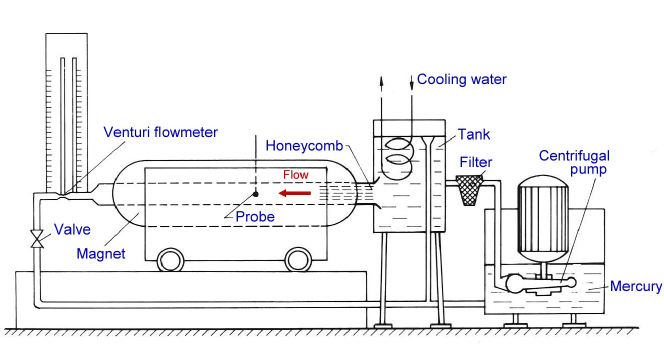
$(b)$

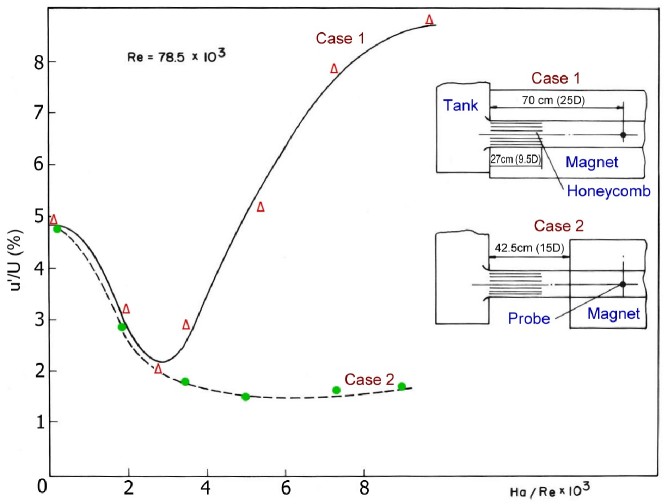
Figure 1: (a), Schematic diagram of the experimental facility of Sukoriansky et al. (1986). (b), Experimental results. Turbulence intensities on the duct axis as functions of $Ha/Re$ at different magnet positions (reprinted with the permission of Springer).

The striking and, at first glance, paradoxical results were obtained in the hot-film measurements of velocity fluctuations 43 cm downstream of the honeycomb’s exit. The measurements showed completely different signals for the two distributions of the magnetic field illustrated in figure 1a. In the situation identified in Sukoriansky et al. (1986) and this paper as Case 1, the entire length (27 cm) of the honeycomb was located between the magnet poles (see the upper schematic illustration in figure 1b), and turbulence was generated and decayed entirely within the practically uniform transverse magnetic field. In the situation identified as Case 2, the magnet poles were shifted downstream so that the axial distance between the honeycomb’s exit and the nearest corner of the pole was 15.5 cm (see the lower schematic illustration in figure 1b). In this case, turbulence was generated at negligible magnetic field and traveled about 5.5 convective times $D/U$ before entering the space between the poles and thus experiencing the full magnetic suppression effect.

The key results are shown in figure 1b reproduced from figure 5 of Sukoriansky et al. (1986). The curves show the turbulence intensity $u^{\prime}/U$ based on the streamwise velocity fluctuations measured on the duct axis 43 cm downstream of the honeycomb, i.e. well in the zone of the uniform magnetic field. The signals measured in the two cases are about the same for weak magnetic fields, approximately at $\mbox{{Ha}}_{D}/\mbox{{Re}}_{D}<3\times 10^{-3}$. Owing to the turbulence suppression by the magnetic field, the intensities decrease with growing $\mbox{{Ha}}_{D}$ reaching $\sim 0.02$ at $\mbox{{Ha}}_{D}/\mbox{{Re}}_{D}=3\times 10^{-3}$. For stronger magnetic fields, however, the signals show entirely different trends. In the case 2, the intensity continues to decrease to about $0.015$ at high $\mbox{{Ha}}_{D}$. In the case 1, the intensity grows rapidly with growing $\mbox{{Ha}}_{D}$ and reaches 0.09 (almost twice the intensity in the flow without magnetic field) at $\mbox{{Ha}}_{D}/\mbox{{Re}}_{D}=10^{-2}$.

The appearance of high-amplitude fluctuations for strong magnetic fields in the case 1 configuration was explained in Sukoriansky et al. (1986) by the effect described above, i.e by development of quasi-two-dimensional flow structures with weak gradients along the magnetic field lines. Such structures would experience weak magnetic suppression and a reduced energy cascade to small length scales thus preserving the strength of the associated velocity fluctuations as the fluid moved downstream. The explanation is consistent with other experiments, e.g. of Kljukin & Kolesnikov (1989). No direct evidence of this scenario has, however, been obtained. The type of the flow structures and the degree of their anisotropy could also not be determined in the experiments and has not been a subject of numerical analysis.

In this paper, we present high-resolution numerical simulations designed to explore validity of the hypothesized scenario leading to the residual velocity fluctuations and to produce a detailed description of the flow. The numerical model reproduces the geometry and parameters of the experiment of Sukoriansky et al. (1986) with one adjustment. For the purpose of understanding the effect of walls on decaying turbulence, two orientations of the transverse magnetic field, along the shorter (as in Sukoriansky et al. (1986)) and longer sides of the duct are considered. The role of the anisotropy introduced by the honeycomb is also addressed. The problem formulation, parameters and numerical procedure are described in section 2. The structure and statistical properties of the computed flows are presented in section 3 . The concluding remarks are provided in section 4.

2 Problem formulation, method and parameters

2.1 Problem formulation

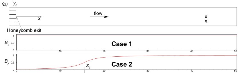
$(b)$ Type A

Type B

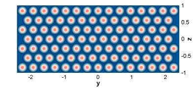
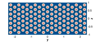
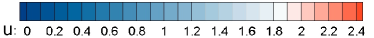
Figure 2: Setting of the problem. (a) Scheme of the computational domain shown in the $x-y$ cross-section. The $x$- and $y$-axes of the coordinate system used in the simulations are shown. The non-dimensional width of the domain in the $z$-direction is 2.0. The profiles of the main component $B$ of the magnetic field computed according to the model of Votyakov et al. (2009) are shown (see text). $x_{1}$ is the location of the upstream corner of the magnet pole-pieces in the case 2. The two crosses in the downstream part of the flow domain indicate the locations where the velocity fluctuation signals are recorded in the experiment of Sukoriansky et al. (1986) and in the simulations. (b) Distribution of the streamwise velocity $u_{inlet}$ imposed at the inlet to imitate the flow exiting the honeycombs of type A and type B (see text).

An isothermal flow of an incompressible electrically conducting Newtonian fluid in a duct of rectangular cross-section is considered. A transverse magnetic field, the exact configuration of which is specified below, is imposed. Assuming the asymptotic limit of low magnetic Reynolds and Prandtl numbers, the quasi-static (non-inductive) approximation of the magnetohydrodynamic interactions (see e.g. Davidson, 2016) is used. The non-dimensional governing equations are

$$\frac{\partial\mbox{\boldmath$v$\unboldmath}}{\partial t}+(\mbox{\boldmath$v$\unboldmath}{\cdot\nabla})\mbox{\boldmath$v$\unboldmath}=-{\nabla p}+\frac{1}{Re}{\nabla}^{2}\mbox{\boldmath$v$\unboldmath}+\frac{\mbox{{Ha}}^{2}}{\mbox{{Re}}}\left(-\nabla\phi\times\mbox{\boldmath$B$\unboldmath}+(\mbox{\boldmath$v$\unboldmath}\times\mbox{\boldmath$B$\unboldmath})\times\mbox{\boldmath$B$\unboldmath}\right),$$ (2)

$$\nabla\cdot\mbox{\boldmath$v$\unboldmath}=0,$$ (3)

$$\nabla^{2}{\phi}=\nabla\cdot({\mbox{\boldmath$v$\unboldmath}\times\mbox{\boldmath$B$\unboldmath}}),$$ (4)

where $v$, $p$, and $\phi$ are the fields of velocity, pressure and electric potential and $B$ is the non-dimensionalized magnetic field. The typical scales used to derive (2)–(4) are the mean streamwise velocity $U$ for velocity, shorter half-width $H$ of the duct for length, $H/U$ for time, $\rho U^{2}$ for pressure, the maximum strength $B_{0}$ of the transverse component for the magnetic field, and $UB_{0}H$ for electric potential. The non-dimensional parameters are the Reynolds number

$$\mbox{{Re}}\equiv\frac{UH}{\nu}$$ (5)

and the Hartmann number

$$\mbox{{Ha}}\equiv B_{0}H\sqrt{\sigma/\rho\nu}$$ (6)

related to the parameters (1) based on the hydraulic diameter as $\mbox{{Re}}=0.3542\mbox{{Re}}_{D}$ and $\mbox{{Ha}}=0.3542\mbox{{Ha}}_{D}$.

We will also use the magnetic interaction parameter

$$\mbox{{N}}\equiv\frac{\mbox{{Ha}}^{2}}{\mbox{{Re}}}=\frac{B_{0}^{2}H\sigma}{\rho U}.$$ (7)

Further settings of the problem are illustrated in figure 2. The computational domain reproduces the test section of the experiment of Sukoriansky et al. (1986). It is a duct segment of length $0\leq x\leq L_{x}$ and cross-section $-L_{y}/2\leq y\leq L_{y}/2$, $-L_{z}/2\leq z\leq L_{z}/2$ with $L_{x}=16\pi$, $L_{y}=4.8$ and $L_{z}=2.0$.

The sidewalls are of zero slip and perfect electric insulation:

$$\mbox{\boldmath$v$\unboldmath}=0,\>\frac{\partial\phi}{\partial n}=0\mbox{ at sidewalls}.$$ (8)

At the inlet $x=0$, we require that

$$\frac{\partial\phi}{\partial x}=0.$$ (9)

A velocity distribution imitating the flow exiting the honeycomb is applied. In the experiment, the tubes of the honeycomb are densely packed and have the inner diameter $d\approx 2.4$ mm and wall thickness about 0.5 mm. The parameters for the flow in a single tube are $\mbox{{Re}}_{d}=6600$ and $\mbox{{Ha}}_{d}=45$ and the non-dimensional pipe length is $L_{d}/d=112.5$. At such parameters, the flow is expected to be weakly turbulent in the case 2. In the case 1, the magnetic field suppresses turbulence and slightly deforms the streamwise velocity profile (see Zikanov et al., 2014a; Müller & Bühler, 2001; Li & Zikanov, 2013). The numerical model ignores the differences and uses the same velocity distribution in the two cases (see figure 2b). The flow in the space between the tubes present in the experiment is also ignored.

To compute the velocity distribution, the inlet plane is covered by hexagons, into which circles of inner diameters and wall thickness corresponding to those of the honeycomb tubes are fitted. The axisymmetric parabolic profile of streamwise velocity is imposed within each tube. At each time step, random three-dimensional velocity perturbations of relative amplitude $10^{-4}$ are added, after which the entire distribution is rescaled so that the mean streamwise velocity is equal to 1.0.

As illustrated in figure 2b, the tubes of the honeycomb can be packed so that they form straight rows along the longer (the honeycomb type A in the following discussion) or shorter (type B) walls of the duct. The results of the simulations presented in section 3.2 demonstrate that the two arrangements produce noticeably different flows.

Soft boundary conditions

$$\frac{\partial\mbox{\boldmath$v$\unboldmath}}{\partial x}=\frac{\partial\phi}{\partial x}=0$$ (10)

are applied at the exit $x=L_{x}$ of the computational domain.

Two orientations of the main component of the magnetic field, parallel to the longer ($B_{y}$) or shorter ($B_{z}$) walls of the duct are used. In each case, the distribution of the magnetic field is approximated in the simulations using the model suggested by Votyakov et al. (2009). The model provides simple formulas for divergence-free, two-dimensional, two-component field created by a magnet with two infinitely wide rectangular pole-pieces. The accuracy of the model was verified in comparison with measurements in Zikanov et al. (2013). The input parameters of the model are the coordinates of the corners of the pole-pieces, for which we take $y=\pm 2.6$ (for $B_{y}$) or $z=\pm 1.2$ (for $B_{z}$), and $x_{1}=-27$, $x_{2}=63$ in the case 1 and $x_{1}=15.5$, $x_{2}=105.5$ in the case 2. The resulting magnetic field has the main component illustrated in figure 2a and the component $B_{x}$, which is much weaker and only significant within the flow domain around the entrance into the magnetic field in the case 2.

The problem is solved numerically using the finite-difference scheme first described as the scheme B in Krasnov et al. (2011) and extended to spatially evolving flows in a duct e.g. in Zikanov et al. (2014b). The solver has been successfully applied in numerous simulations of turbulent and transitional MHD flows at high Re and Ha (see e.g. Zikanov et al., 2014a; Krasnov et al., 2013, 2012; Zikanov et al., 2014b; Li & Zikanov, 2013). The scheme is explicit and of the second order in time and space. The discretization is on the structured collocated grid built along the lines of the Cartesian coordinate system. The exact conservation of mass, momentum, and electric charge, as well as near-conservation of kinetic energy are achieved by using the velocity and current fluxes obtained by interpolation to staggered grid points. The standard projection technique is applied to compute pressure and enforce incompressibility. The numerical algorithm is parallelized using the hybrid MPI-OpenMP approach.

The modification of the algorithm in comparison with the original version of Krasnov et al. (2011) concerns the solution of the Poisson equations for pressure and electric potential. The fast cosine decomposition is used in the streamwise direction, for which the right-hand side of the equation is modified to achieve homogeneous Neumann boundary conditions at $x=0$ and $x=L_{x}$. The direct cyclic reduction solver implemented in the subroutines of the library FishPack (Adams et al., 1999) is used in the $y-z$-plane.

The computational results reported below are obtained on the grid consisting of $N_{x}\times N_{y}\times N_{z}=3072\times 512\times 192$ points. The points are clustered towards the duct’s walls using the coordinate transformation

$$y=\frac{L_{y}}{2}\left[0.9\sin\left(\frac{\pi}{2}\eta\right)+0.1\eta\right],\>z=\frac{L_{z}}{2}\left[0.9\sin\left(\frac{\pi}{2}\zeta\right)+0.1\zeta\right],$$ (11)

where $-1\leq\eta\leq 1$ and $-1\leq\zeta\leq 1$ are the transformed coordinates, in which the grid is uniform.

A grid sensitivity study was performed to determine that the model sufficiently accurately reproduced the essential features of the flow, such as mixing and instabilities of the honeycomb jets, generation of turbulence, and its decay in the presence of the magnetic field. Additional simulations for the case 1 and case 2 configurations with the magnetic field parallel to the longer sides of the duct on the smaller grid with $N_{x}\times N_{y}\times N_{z}=2048\times 384\times 128$ and the same clustering scheme were carried out. The results were qualitatively the same as on the larger grid with minor quantitative differences. In particular, the time-averaged wall friction coefficients computed for the entire flow domain changed by less than 1%. The effect of the numerical resolution on the results is further discussed in section 4.

Several additional tests were performed at $\mbox{{Ha}}=0$ to analyze the effect of the grid size, grid clustering, and the amplitude of the noise added at the inlet on the instability and mixing of jets in the portion of the duct just downstream of the inlet. It has been found that at the grid clustering associated with (11) further increase of the grid size and further decrease of the noise amplitude do not result in visible changes in the formation of turbulence.

3 Results

The parameters of the simulations are listed in Table 1. For convenience of the readers, the runs are numbered such that odd indices 1,3,5,7 correspond to case 1 with homogeneous field, whereas even indices 2,4,6,8 – to case 2 with non-homogeneous field (see Fig. 2a). Each simulation is initialized with a laminar state and continued for $100$ non-dimensional time units, whereby a fully developed flow is established. Subsequently, the simulation is continued for a “production phase” of $100$ (in the runs 1-4) or $50$ (in the runs 5-8) time units. The turbulence statistics in this paper are based on the, respectively, $1000$ or $500$ flow samples collected during this phase with the time interval $0.1$.

The simulations $1$ and $2$ are for $\mbox{{Ha}}/\mbox{{Re}}=\mbox{{Ha}}_{D}/\mbox{{Re}}_{D}=2.0\times 10^{-3}$, i.e., for the parameters in the range of moderate magnetic fields where a strong (two-fold) reduction of turbulence intensity was detected in the experiment of Sukoriansky et al. (1986) for both the field configurations (see figure 1b). The simulations $3$-$8$ are for $\mbox{{Ha}}/\mbox{{Re}}=\mbox{{Ha}}_{D}/\mbox{{Re}}_{D}=7.0\times 10^{-3}$. For this strong magnetic field, the experiment shows anomalous behavior with the turbulence intensity in the case 2 configuration remaining low, but the intensity in the case 1 configuration growing to a level about 50% higher than without the magnetic field.

In the following discussion, the properties of the computed flows are analyzed using the fields of turbulent fluctuations defined as

$$\mbox{\boldmath$v$\unboldmath}^{\prime}=\mbox{\boldmath$v$\unboldmath}-\langle\mbox{\boldmath$v$\unboldmath}\rangle,$$ (12)

where $\langle\mbox{\boldmath$v$\unboldmath}\rangle(\mbox{\boldmath$x$\unboldmath})$ is the mean velocity obtained by time-averaging over the entire production phase of the run.

	Field	Field	Honeycomb
Run #	Orientation	Configuration	Type	Re	Ha	$\mbox{{N}}=\frac{\mbox{{Ha}}^{2}}{\mbox{{Re}}}$	$R=\frac{\mbox{{Re}}}{\mbox{{Ha}}}$
1	$B_{y}$	Case 1	A	27800	55	0.1088	505.5
2	$B_{y}$	Case 2	A	27800	55	0.1088	505.5
3	$B_{y}$	Case 1	A	27800	195	1.368	142.6
4	$B_{y}$	Case 2	A	27800	195	1.368	142.6
5	$B_{z}$	Case 1	A	27800	195	1.368	142.6
6	$B_{z}$	Case 2	A	27800	195	1.368	142.6
7	$B_{z}$	Case 1	B	27800	195	1.368	142.6
8	$B_{z}$	Case 2	B	27800	195	1.368	142.6

Table 1: Simulation parameters.

We start the discussion with the main results summarized in Table 2. The time-averaged root-mean-square amplitudes of the velocity fluctuations computed at $x=43$, $z=0$ and two values of $y$ are shown. The values for $u^{\prime}$ correspond to the experimental measurements of Sukoriansky et al. (1986) (see figure 1b) and show that the seemingly paradoxical dependence of the fluctuation amplitude on the strength of the magnetic field and magnet’s location is reproduced by the simulations. Weak fluctuations of all the velocity components are found in the runs 1 and 2 performed at $\mbox{{Ha}}=55$. Equally weak fluctuations are found in the runs 4, 6, and 8 performed at $\mbox{{Ha}}=195$ when the poles of the magnet shifted downstream (the case 2 configuration in figure 2). Anomalously high fluctuation amplitudes are found in the runs 3, 5, and 7, i.e. in the flows with $\mbox{{Ha}}=195$ and the honeycomb exit located within the zone of uniform magnetic field (the case 1 configuration in figure 2). The amplitudes of two velocity components are increased: the streamwise component $u^{\prime}$ and the component orthogonal to the magnetic field ($w^{\prime}$ in the run 3 and $v^{\prime}$ in the runs 5 and 7). The increase in comparison to the other cases is about four-fold in the runs 3 and 7 and two-fold in the run 5.

Table 2 shows that the flow’s behaviour is affected by the magnetic field strength, magnet location, orientation of the magnetic field with respect to the duct walls, and the honeycomb arrangement. The following discussion is separated into two parts. The mechanism of the generation of high-amplitude fluctuations is explained and illustrated in section 3.1 on the basis of the results obtained in the runs 1-4. Further investigation of the fluctuations is presented in section 3.2, where the influence of the magnetic field orientation and honeycomb arrangement is analyzed using the data from the runs 5-8.

A comment is in order concerning the comparison between the simulations and the experiments of Sukoriansky et al. (1986). As we have already mentioned and discuss in detail below, the qualitative agreement is quite satisfactory. The quantitative agreement is, however, poor. From table 2 and figure 1b and figure 6 of Sukoriansky et al. (1986) we see that in all the simulations the computed rms fluctuations are about five times lower than in the experiment. Possible reasons for this are discussed in section 4.

Run #	center ($y=0$)			off center ($y=-1.4$)
	$u^{\prime}$	$v^{\prime}$	$w^{\prime}$	$u^{\prime}$	$v^{\prime}$	$w^{\prime}$
1	$4.35\times 10^{-3}$	$3.90\times 10^{-3}$	$3.47\times 10^{-3}$	$4.40\times 10^{-3}$	$4.41\times 10^{-3}$	$3.79\times 10^{-3}$
2	$4.67\times 10^{-3}$	$4.55\times 10^{-3}$	$3.55\times 10^{-3}$	$4.82\times 10^{-3}$	$5.23\times 10^{-3}$	$4.12\times 10^{-3}$
3	$1.35\times 10^{-2}$	$4.45\times 10^{-3}$	$1.13\times 10^{-2}$	$1.35\times 10^{-2}$	$4.30\times 10^{-3}$	$1.21\times 10^{-2}$
4	$3.35\times 10^{-3}$	$2.65\times 10^{-3}$	$2.38\times 10^{-3}$	$4.11\times 10^{-3}$	$2.56\times 10^{-3}$	$2.78\times 10^{-3}$
5	$5.30\times 10^{-3}$	$5.40\times 10^{-3}$	$1.61\times 10^{-3}$	$5.62\times 10^{-3}$	$5.75\times 10^{-3}$	$1.61\times 10^{-3}$
6	$3.76\times 10^{-3}$	$3.87\times 10^{-3}$	$1.87\times 10^{-3}$	$3.84\times 10^{-3}$	$3.27\times 10^{-3}$	$2.78\times 10^{-3}$
7	$1.23\times 10^{-2}$	$1.05\times 10^{-2}$	$3.46\times 10^{-3}$	$1.18\times 10^{-2}$	$1.25\times 10^{-2}$	$3.59\times 10^{-3}$
8	$5.03\times 10^{-3}$	$4.66\times 10^{-3}$	$1.48\times 10^{-3}$	$5.17\times 10^{-3}$	$4.69\times 10^{-3}$	$2.81\times 10^{-3}$

Table 2: RMS amplitudes of fluctuations of velocity components at the points $x=43$, $z=0$, $y=0$ (center) and $x=43$, $z=0$, $y=-1.4$ (off center) computed using the entire signals of fully developed flow. Since the time-averaged streamwise velocity at these points is about 1.0 in our units, the values approximately correspond to the respective turbulence intensities. The data for flows with anomalously high fluctuation amplitudes are marked by gray colour.

3.1 Effect of magnetic field on turbulence decay

The following discussion is primarily based on simulations 1-4.

3.1.1 Velocity fluctuations

Figure 3 shows the time signals of the velocity components computed at the point $x=43$, $y=z=0$ corresponding to the point of velocity measurements in the experiment of Sukoriansky et al. (1986) (see figure 1b). The rms amplitudes listed in table 2 are calculated using these signals and similar signals recorded at $x=43$, $y=-1.4$, $z=0$. We see that the behaviour indicated by the rms data is not subject to significant variations at long time scales. Consistent anomalously high fluctuation amplitudes of streamwise ($u$) and field-normal transverse ($w$) velocity components are found in the run 3 when the magnetic field is strong and has the case 1 configuration.

$\mbox{{Ha}}=55$

$\mbox{{Ha}}=195$

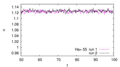
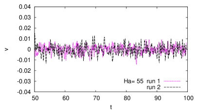
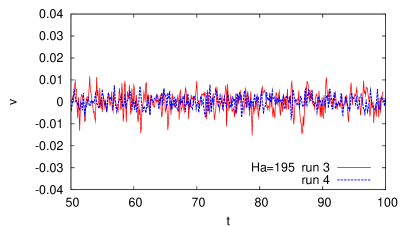
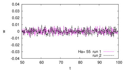
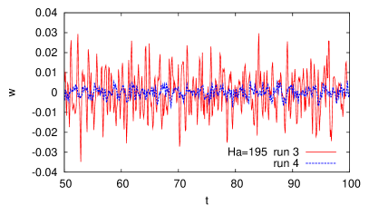
Figure 3: Time signals of velocity components computed at $x=43$, $z=0$ and $y=0$ shown for the second half of the fully developed flow stages of the simulations 1-4. Runs 1,2 at $\mbox{{Ha}}=55$ and runs 3,4 at $\mbox{{Ha}}=195$ are shown in, respectively, left and right columns. From top to bottom: streamwise $u$, spanwise $v$ (transverse and parallel to the main component of the magnetic field) and vertical $w$ (transverse and perpendicular to the main component of the magnetic field) velocity components.

3.1.2 Flow structure

Run 1

Run 2

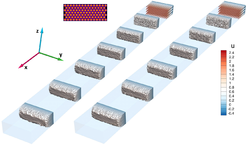
Run 3

Run 4

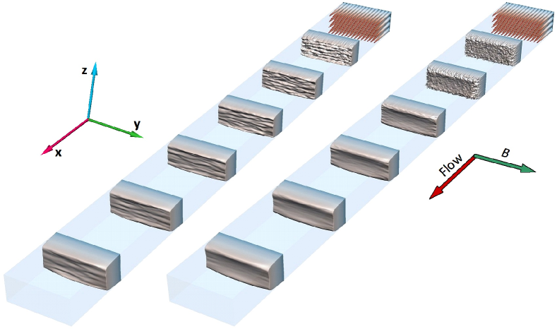
Figure 4: Instantaneous distributions of the streamwise velocity $u$ at several locations along the duct shown for the fully developed flows in the simulations 1-4 (see table 1 for the flow parameters).

Run 3

Run 4

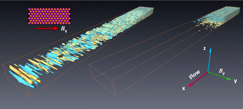
Figure 5: Isosurfaces of the vertical velocity component $w$ (transverse and perpendicular to the main component of the magnetic field $B_{y}$) for the runs 3 and 4. Two iso-levels of the same magnitude and opposite signs (yellow – positive, blue – negative) are visualized. The insert on the left shows the honeycomb pattern and the main component of the magnetic field $B_{y}$.

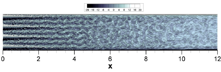
Figure 6: Instantaneous distribution of the vorticity component $\omega_{y}$ parallel to the magnetic field in the $(x,z)$ cross-section through the duct’s axis. The transformation of jets into vortices is shown for the run 3 by a close-up of the inlet region at $0\leq x\leq 12$.

The spatial structures of the fully developed flows in the simulation runs 1-4 are illustrated in figures 4 and 5. We see that at $\mbox{{Ha}}=55$ (runs 1 and 2 in figure 4) the flows remain turbulent, although the velocity fields are significantly modified by the magnetic fields. The modifications include development of the mean flow profile with a nearly flat core and characteristic Hartmann and sidewall boundary layers (see figure 4) and reduction of turbulence intensity. Since the Reynolds number based on the Hartmann thickness $R\equiv\mbox{{Re}}/\mbox{{Ha}}=505$, this result is in agreement with the earlier studies of the flows in long ducts with uniform transverse magnetic field. As discussed, for example, in the review by Zikanov et al. (2014a), fully laminar and fully turbulent flows are typically found at, respectively, $R<200$ and $R>400$, with the transitional range at $200<R<400$. We also note that at $\mbox{{Ha}}=55$ no substantial differences are observed between the case 1 and case 2 configurations except that the flow modification happens farther downstream in the run 2.

In the simulations 3 and 4 performed at $\mbox{{Ha}}=195$, we have $R=143$, which is below the laminar-turbulent transition range. Turbulence is, therefore, suppressed (albeit not completely, as we will see in the following analysis) as the fluid moves through the magnetic field (see figure 4). The flows obtained for the two configurations of the magnetic field are, however, clearly different.

In the case 2 configuration, there is a distance between the honeycomb and the beginning of the zone of full-amplitude magnetic field. The plots for the run 4 in figures 4 and 5 clearly show that the distance is sufficient for the instability and mixing of the jets generated by the honeycomb. Three-dimensional turbulence develops. Upon entering the magnetic field, the turbulent fluctuations are quickly suppressed, which is reflected by the strong reduction of the rms velocity fluctuations at $x=43$ shown in table 2.

In the case 1 configuration, the formation of turbulence near the honeycomb exit occurs in the presence of a full-amplitude magnetic field. As shown in figures 4 and 5, the velocity field in the run 3 quickly becomes strongly anisotropic. The instability of the honeycomb jets does not lead to a three-dimensional turbulent state, but to a quasi-two-dimensional flow dominated by structures aligned with the magnetic field.

The illustrations in figures 4 and 5, the distribution of the vorticity component $\omega_{y}$ parallel to the magnetic field in the $(x,z)$ cross-section of the duct shown in figure 6, and the additional visualizations analyzed in the course of our work (not shown) suggest the following scenario of the evolution of the spatial structure of the flow. In the inlet portion of the duct, approximately at $x<3$, the dominant feature of the evolution is the transformation of the round jets exiting the honeycomb into quasi-two-dimensional planar (nearly parallel to the $(x,y)$ plane) jets. Already in the course of this transformation, the jets experience the Kelvin-Helmholtz instability that leads to noticeable waviness at $x$ between $3$ and $4$ and to roll-up into quasi-two-dimensional vortices at around $x=5$. The following evolution is characterized by quasi-two-dimensional vortices superimposed on the plug-like profile of the streamwise velocity. It is indicated by figures 4-6 and confirmed by the quantitative analysis presented later in this paper that the dynamics of the vortices is that of quasi-two-dimensional turbulence.

The last preceding paragraph summarizes our key observation. It provides the basis for the explanation suggested earlier for the anomalously strong velocity fluctuations observed in the experiments of Sukoriansky et al. (1986) and, likely, other experiments such as those of Kljukin & Kolesnikov (1989). Due to their weak gradients along the magnetic field lines, the quasi-two-dimensional vortices do not generate strong Joule dissipation. Furthermore, the quasi-two-dimensionality reduces the energy flux from large to small length scales, which implies weaker viscous dissipation. The flow structures are still suppressed by the Joule and viscous dissipation in the boundary layers, but the effect is not strong. The quasi-two-dimensional vortices are visible till the end of the flow domain (see figures 4 and 5), and are responsible for the generation of high-amplitude velocity fluctuations at far downstream locations.

3.1.3 Turbulence decay along the duct

The distributions of the turbulent kinetic energy in each velocity component $\langle{u^{\prime}}^{2}\rangle$, $\langle{v}^{2}\rangle$, $\langle{w}^{2}\rangle$ are computed as functions of $x$ along the lines $y=z=0$ and $y=-1.4$, $z=0$.

The turbulence decay curves obtained at $y=z=0$ are shown in figures 7 and 8. The intervals $0\leq x<0.1$ in figure 7 and $0\leq x<1$ in figure 8 are excluded to highlight the decay stage of the flow evolution and to eliminate the initial stage of jet instability and mixing, at which the data are strongly influenced by the position of the point $y=z=0$ with respect to the honeycomb pattern. The slope lines are plotted to illustrate the decay rate rather than to suggest a specific scaling.

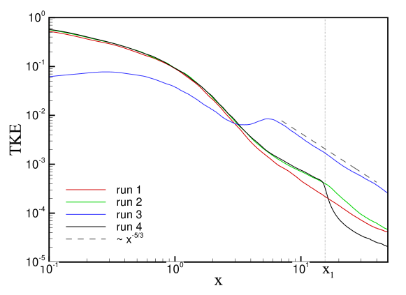
Figure 7: Time-averaged turbulent kinetic energy $\langle{u^{\prime}}^{2}+{v^{\prime}}^{2}+{w^{\prime}}^{2}\rangle$ as a function of $x$ along the centerline of the duct $y=z=0$. The vertical dotted line indicates the location of the corners of the magnet pole-pieces in the runs 2 and 4. The slope line $\sim x^{-5/3}$ is shown for comparison.

(a)

(b)

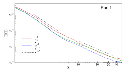
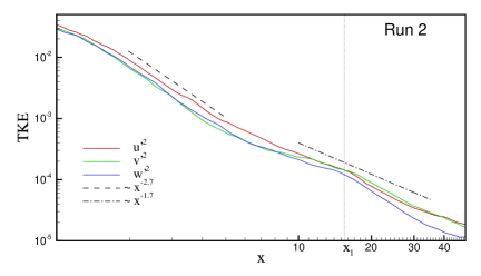
(c)

(d)

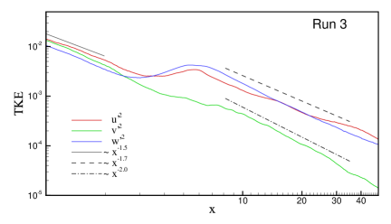
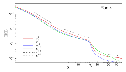
Figure 8: Time-averaged turbulent kinetic energies in separated velocity components $\langle{u^{\prime}}^{2}\rangle$, $\langle{v^{\prime}}^{2}\rangle$, $\langle{w^{\prime}}^{2}\rangle$ as functions of $x$ along the centerline of the duct $y=z=0$. The inlet section of the duct $0\leq x\leq 1$ is excluded. Slope lines are shown for comparison. The vertical dotted line indicates the location of the corners of the magnet pole-pieces in the runs 2 and 4.

For the runs 1 and 2, the energy decay curves obtained at two locations of the magnet are not very different from each other. This suggests weak influence of the magnetic field in agreement with the low magnetic interaction parameter $\mbox{{N}}=0.1088$. For small $x$, the magnetic damping causes somewhat more rapid decay in the run 1 than in the run 2. At larger $x$, approximately at $x>x_{1}$ where the strength of the magnetic field is about the same in the two flows, turbulence decays faster for the run 2. We attribute that to the stronger Joule dissipation caused by the stronger velocity gradients in the field direction retained by the flow. At the end of the duct, the turbulent kinetic energy in the two flows decreases to approximately the same level.

The curves in figure 8a,b show significant level of fluctuations in all three velocity components. This is in agreement with the three-dimensional fully turbulent nature of the flow visualized in figure 4. At the same time, the Reynolds stress tensor is not isotropic. At small $x$, $\langle{u^{\prime}}^{2}\rangle>\langle{v^{\prime}}^{2}\rangle\sim\langle{w^{\prime}}^{2}\rangle$. At larger $x$, approximately at $x>12$ in the flow 1 and $x>20$ in the flow 2, we see significant anisotropy with $\langle{u^{\prime}}^{2}\rangle\sim\langle{v^{\prime}}^{2}\rangle>\langle{w^{\prime}}^{2}\rangle$.

The effect of the magnetic field is much more pronounced in the flows 3 and 4. For the run 4, the energy decay curves is practically indistinguishable from those for the run 2 curve for $x<x_{1}$ (see figure 7). For $x>x_{1}$, the strong imposed magnetic field results in rapid decay and the lowest value of the turbulent kinetic energy at the duct exit among all the simulations 1-4. Interestingly, during the initial stages of this decay, in the interval $15<x<30$, the fluctuations of the velocity component $v$ parallel to the magnetic field remain stronger than the fluctuations of the other two components (see figure 8d). We do not have data that would allow us to precisely identify the specific flow structures responsible for this effect. We note that the behaviour is consistent with the evolution of homogeneous, initially isotropic turbulence after sudden application of a strong magnetic field. As predicted by Moffatt (1967) and confirmed by Burattini et al. (2010) and Favier et al. (2010), the initial stages of the decay are characterized by the energy of field-parallel velocity fluctuation component substantially larger (two times larger in the asymptotic limit $\mbox{{N}}\gg 1$) than the energy of the field-perpendicular components. Far downstream, approximately for $x>30$, the remaining fluctuations $u^{\prime}$ and $w^{\prime}$ decay very slowly, with the rate approaching $\langle{u^{\prime}}^{2}\rangle\sim\langle{w^{\prime}}^{2}\rangle\sim x^{-0.5}$.

For the most interesting simulation 3, figures 7 and 8 show a very strong effect of the magnetic field. In the entrance portion of the duct, the generation of turbulence is inhibited and the turbulent kinetic energy is an order of magnitude smaller than in the other three cases. The energy grows slightly for $x<0.3$ and then decays, but much slower than in the other cases. The energy becomes larger than in the other flows at $x\approx 3$.

Interesting behaviour is observed in the interval $3<x<6$. While the fluctuation energy $\langle{v^{\prime}}^{2}\rangle$ of the field-parallel velocity component continues to decay along the duct, the fluctuation energies of the other two components grow. This behaviour manifests substantial energy transfer from the mean flow to the fluctuations. The visualizations of the flow structure in figures 4-6 allow us to attribute it to the Kelvin-Helmholtz instability of the quasi-two-dimensional planar jets, which develop quite rapidly at already $x\approx 3$, and the resulting formation of quasi-two-dimensional vortices.

The turbulence decay at $x>6$ is characterized by $\langle{u^{\prime}}^{2}\rangle\sim\langle{w^{\prime}}^{2}\rangle\gg\langle{v^{\prime}}^{2}\rangle$ (see figure 8c), which is expected for quasi-two-dimensional vortical structures extending wall-to-wall in the field direction. The energy remains much larger than in the other three flows. For $x>8$, the decay is well approximated by the power law $\sim x^{-5/3}$ (see figure 7). It should be stressed that we do not have theoretical arguments supporting this decay rate. The same is true for the decay rates indicated by the slope lines in figure 8. The lines are shown purely for comparison, as illustrations of the decay trends obtained in the simulations.

3.1.4 Turbulence statistics

The velocity fields computed in the runs 1-4 for fully developed flows at $100<t<200$ are used to accumulate the turbulence statistics discussed in this section. Energy power spectra are calculated from the velocity fluctuation signals at $x=43$, $y=z=0$ (see figure 3). To comply with the periodicity condition, we have used a window function $w(\tau)$, based on a superposition of two hyperbolic tangents $w(\tau)=\tanh(a\tau^{3})+\tanh(a(T_{m}-\tau)^{3})-1$ with $a=0.03$. Here it is assumed that the argument $\tau$ varies from $0$ to the maximum $T_{m}=100$. This function provides smooth transition from zero to unity at both ends and retains more than 90% of the unmodified sequence.

A possible alternative to this approach would be to compute the spatial wavenumber spectra in the cross-section $x=const$. For that, we would have to use the data recorded in the core (excluding the boundary layers) portion of the cross-section. The data would have to be interpolated to a uniform grid and time-averaged. We see our approach as preferable for the following several reasons. It is free from the errors associated with the interpolation and the variation of flow properties in the cross-section. The spectra based on the time signal directly correspond to the measurements made in the experiment. Finally, one-dimensional spectra are more informative in the case of strongly anisotropic turbulence than three-dimensional or two-dimensional ones.

The spectra are shown in figure 9. We see that even at $\mbox{{Ha}}=195$ the spectra are continuously populated in a wide range of frequencies $\omega$, so the flows can be classified as turbulent. The inertial ranges cannot be reliably determined due to their shortness typical for turbulence decay in the presence of MHD suppression. Still, one sees portions of the spectra with the slope close to $\sim\omega^{-5/3}$ at $\mbox{{Ha}}=55$ and $\sim\omega^{-3}$ at $\mbox{{Ha}}=195$. The latter can be viewed as an indication of the quasi-two-dimensional character of the turbulence, although, as argued by Alemany et al. (1979) and Sommeria & Moreau (1982), the same spectrum may appear as a result of the equilibrium between the local angular energy transfer and the Joule dissipation in the core flow or the Hartmann boundary layers.

(a)

(b)

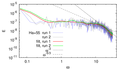
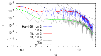
(c)

(d)

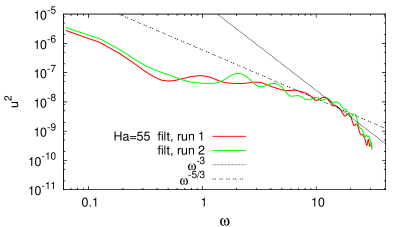
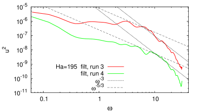
(e)

(f)

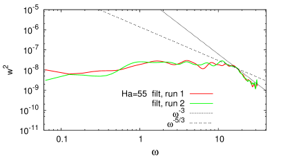
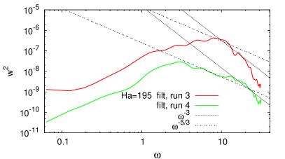
Figure 9: Power spectra of the kinetic energy based on the velocity signals computed at $x=43$, $y=z=0$ in the fully developed flows at $\mbox{{Ha}}=55$ (runs 1,2 shown in the left column) and $\mbox{{Ha}}=195$ (runs 3 and 4 shown in the right column). The spectra of the total kinetic energy $E=u^{2}+v^{2}+w^{2}$ and the energy in two velocity components $u$ and $w$ are shown. For the sake of clarity, the filtered spectra (using Bezier spline) are shown, the original raw data are only demonstrated on plots (a,b). Also shown, for the sake of comparison, are the power laws $\sim\omega^{-3}$ and $\sim\omega^{-5/3}$. The spectra of the energy in the velocity component $v$ (not shown) demonstrate practically no difference between the four flows.

The spectrum of $w^{2}$ is particularly convenient for characterization of the anomalous high-amplitude turbulent fluctuations observed in the flow 3 (see figure 9f). The energy peak at $\omega\approx 10$ is evidently associated with the characteristic streamwise size of the vortices (see figure 5).

(a)

(b)

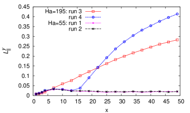
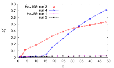
(c)

(d)

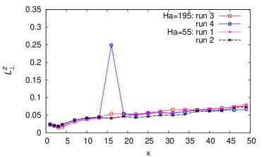
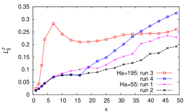
Figure 10: Integral length scales based on the correlation data obtained in the runs 1-4: $(a,b)$ parallel to the magnetic field, $(c,d)$ perpendicular to the field. The scales $L_{\parallel}^{y}$, $L_{\perp}^{y}$ and $L_{\parallel}^{z}$, $L_{\perp}^{z}$ are shown as functions of the streamwise coordinate $x$. The nature of the peak at $x=16$ in figure $(c)$ is explained in appendix A.

We have also evaluated two-point velocity correlation functions along the direction parallel ($y$) and perpendicular ($z$) to the magnetic field. The coefficients are defined as (here for the velocity component $w$)

$$R^{w}(\ell_{y}) = \frac{\int_{-L_{z}+\delta_{z}}^{L_{z}-\delta_{z}}w(x^{*},0,z)w(x^{*},\ell_{y},z)dz+\int_{-L_{z}+\delta_{z}}^{L_{z}-\delta_{z}}w(x^{*},0,z)w(x^{*},-\ell_{y},z)dz}{2\int_{-L_{z}+\delta_{z}}^{L_{z}-\delta_{z}}w^{2}(x^{*},0,z)dz}$$ (13)

$$R^{w}(\ell_{z}) = \frac{\int_{-L_{y}+\delta_{y}}^{L_{y}-\delta_{y}}w(x^{*},y,0)w(x^{*},y,\ell_{z})dy+\int_{-L_{y}+\delta_{y}}^{L_{y}-\delta_{y}}w(x^{*},y,0)w(x^{*},y,-\ell_{z})dy}{2\int_{-L_{y}+\delta_{y}}^{L_{y}-\delta_{y}}w^{2}(x^{*},y,0)dy}.$$ (14)

The magnetohydrodynamic boundary layers of thicknesses $\delta_{y}=L_{y}/\mbox{{Ha}}$ and $\delta_{z}=L_{z}/\mbox{{Ha}}^{1/2}$ are excluded from the integration, so the estimation of the correlations is limited to the zone of approximately homogeneous turbulence in the core flow. The integrals are calculated at the time moments separated by $0.1$ and time-averaged over the period of fully developed flow. The calculations are performed for several duct’s cross-sections $x=x^{*}$, namely at $x^{*}=1,2,3,4$ and at $7\leq x^{*}\leq 49$ with a step of $3$.

The computed correlation curves provide detailed information on the development of the dimensional anisotropy along the duct. The results are presented in appendix A. Here, we discuss the longitudinal ($L_{\|}$) and transverse ($L_{\bot}$) length scales along ($y$) and across ($z$) the magnetic field derived as:

$$L_{\|}^{y} = \int_{0}^{1-\delta_{y}}R^{v}(\ell_{y})d\ell_{y},$$ (15)

$$L_{\bot}^{y} = \int_{0}^{1-\delta_{y}}R^{w}(\ell_{y})d\ell_{y},$$ (16)

$$L_{\|}^{z} = \int_{0}^{1-\delta_{z}}R^{w}(\ell_{z})d\ell_{z},$$ (17)

$$L_{\bot}^{z} = \int_{0}^{1-\delta_{z}}R^{v}(\ell_{z})d\ell_{z}.$$ (18)

In isotropic turbulence, we would find $L_{\|}^{y}\approx L_{\|}^{z}\approx 2L_{\bot}^{y}\approx 2L_{\bot}^{z}$. These relationships are, quite expectedly, not satisfied by the flows 3 and 4 with strong magnetic field. For the flows 1 and 2 with weak magnetic field, the relationships hold for $L_{\|}^{z}$ and $L_{\bot}^{z}$ at large distances from the inlet, where the honeycomb-created jets are properly mixed (see figures 10c and d), but not for $L_{\|}^{y}$ and $L_{\bot}^{y}$ (not clearly visible in figures 10a and b, but verified in our analysis). We also see that at weak magnetic field the scales $L_{\|}^{y}$ and $L_{\bot}^{y}$ remain practically constant, while $L_{\|}^{z}$ and $L_{\bot}^{z}$ grow downstream. The outlying point in figure 10c corresponds to the effect of the local flow transformation in the run 4 discussed in appendix A.

In the runs 3 and 4, the strong magnetic field causes rapid growth of $L_{\|}^{y}$, $L_{\bot}^{y}$, and $L_{\|}^{z}$, but not $L_{\bot}^{z}$. The most interesting for us are the length scales $L_{\bot}^{y}$ and $L_{\|}^{z}$ computed on the basis of the fluctuations of the velocity component $w$. We see that the length scale $L_{\bot}^{y}$ along the magnetic field grows monotonically downstream after the full-strength magnetic field is introduced (at $x=0$ in the run 3 and at $x=x_{1}$ in the run 4) as an indication of flow’s transition into strongly anisotropic form. Interestingly, the large vortices developing in the flow 3 result in slower growth, so at the end of the domain, $L_{\bot}^{y}$ is smaller than in the flow 4. The length scale $L_{\|}^{z}$ in the direction perpendicular to the magnetic field grows very rapidly at small $x$ in the flow 3 and stabilizes at about $0.25$ at $x$ above approximately $20$. This value as associated with the typical transverse size of the quasi-two-dimensional vortices. On the contrary, in the flow 4, where the vortices do not form, $L_{\|}^{z}$ grows continuously downstream.

3.2 Effect of walls and anisotropy of inlet conditions

The discussion of section 3.1 as well as previous works by various authors (see e.g. Moffatt, 1967; Sukoriansky et al., 1986; Kljukin & Kolesnikov, 1989; Burattini et al., 2010) suggest that the development and persistence of quasi-two-dimensional structures aligned with the strong imposed magnetic field is a general physical phenomenon to be observed, in some form, in all decaying MHD turbulent flows. At the same time, features of the flow’s configuration may strongly affect the realization of the phenomenon in a specific case. For our system, the most important such features are: (i) the location of the duct’s walls non-parallel to the magnetic field, which limit the longitudinal size of the quasi-two-dimensional flow structures and (ii) the design of the honeycomb, which may introduce anisotropy into the initial state of the flow.

The importance of these features is due to the presence of the strong transverse magnetic field. Without the field, approximately homogeneous and isotropic turbulence insensitive to such details of the system’s geometry is expected to form in the core of the duct downstream of the honeycomb’s exit.

The two effects are explored in our study in the simulation runs 5-8 (see table 1 for parameters). The strong magnetic field corresponding to $\mbox{{Ha}}=195$ is applied in all the simulations, so we expect the behaviour similar to that observed earlier in the simulations 3 and 4. The main component of the magnetic field is oriented along the shorter side of the duct ($B_{z}$) and not along the longer side as before. The case 1 and case 2 distributions of the magnetic field along the duct are considered. In addition to allowing us to see the effect of the distance between the field-crossing walls, the new simulations provide a direct comparison with the experiment of Sukoriansky et al. (1986), in which the magnetic field is in the $z$-direction.

Two arrangements of the honeycomb tubes are considered. As illustrated in figure 2b, the tubes are arranged into straight rows along the longer (Type A) or shorter (Type B) sides of the duct. This implies different anisotropies of the flows exiting the honeycomb. The type A (runs 5 and 6) produces structures with weaker average gradients in the $y$-direction, i.e. perpendicularly to the magnetic field. The type B (runs 7 and 8) results in the flow structures with weaker gradient in the $z$-direction, i.e. the direction of the magnetic field.

The rms velocity fluctuations in fully developed flows are presented in table 2. We see that the situation is generally similar to that observed earlier in the simulations 3 and 4. The anomalously strong velocity fluctuations appear when the magnetic field has the configuration of case 1 (runs 5 and 7) but not of case 2 (runs 6 and 8). Also as before, the strong fluctuations develop in the streamwise velocity component $u$ and the transverse component perpendicular to the magnetic field $v$.

The effect of the anisotropy introduced by the honeycomb is clearly visible. The fluctuation amplitude in the run 7 is about the same as in the run 3, while it is about two times smaller in the run 5.

Run 5

Run 6

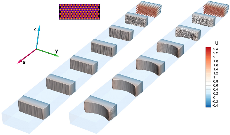
Run 7

Run 8

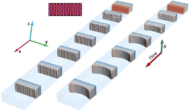
Figure 11: Instantaneous distributions of the streamwise velocity $u$ at several locations along the duct shown for the fully developed flows in simulations 5-8 (see table 1 for flow parameters).

Run 5

Run 6

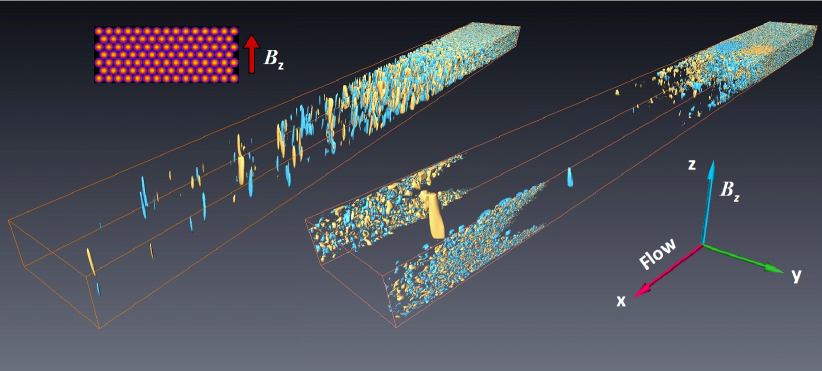
Run 7

Run 8

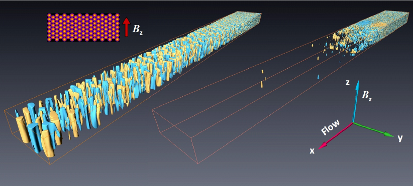
Figure 12: Isosurfaces of the velocity component $v$ (transverse and perpendicular to the main component of the magnetic field $B_{z}$) for the simulations 5, 6 (top) and 7,8 (bottom). Two iso-levels of the same magnitude and opposite signs (yellow – positive, blue – negative) are visualized. The insert on the left shows the honeycomb patterns of Type A and B, and the main component of the magnetic field $B_{z}$.

To explain these results, we will consider the spatial structure of the flows visualized in figures 11–12. As in section 3.1, profiles of the streamwise velocity (figure 11) and isosurfaces of the transverse velocity component perpendicular to the magnetic field (figure 12) are shown.

We start with the simulations 6 and 8, in which the magnet poles are shifted downstream of the honeycomb exit (the case 2 configuration, see figures 1b and 2a). One can see that, similarly to the simulation 4, three-dimensional turbulence forms before the fluid enters the zone of strong magnetic field. Subsequent effective magnetic damping results in the low amplitude of remaining velocity fluctuations reported in table 2.

The flows of the simulations 6 and 8 also have prominent M-shaped profiles of streamwise velocity (see figure 11). Such a profile is expected when the flow in a duct with electrically insulating walls enters the zone of strong transverse magnetic field (see e.g. Branover, 1978; Andreev et al., 2006). The profile can also be noticed in the run 4 (see figure 4), but it is more pronounced in the runs 6 and 8 due to the larger distance between the sidewalls (the walls parallel to the magnetic field).

The two just discussed flow features are equally observed in the simulations 6 and 8. The only difference between the two flows is that we see significant velocity fluctuations near the sidewalls in the far downstream portion of the duct in the flow 6 but not in flow 8 (see figures 11 and 12). The physical nature of this phenomenon has been verified in additional simulations. We attribute its existence to the strong shear layer associated with the planar side-wall jets forming in the M-shaped profile. Such layers are known to be be very susceptible to instabilities (see e.g. Kobayashi et al., 2012). Similar phenomenon is also known in another configuration with planar side-wall jets, as Hunt’s flow (Braiden et al., 2016). The fact that side-wall turbulence appears in the run 6, but not in the run 8, is the effect of the honeycomb arrangement. Stronger flow instability is triggered in the run 6, since the perturbations introduced into the side-wall layers by the honeycomb of type A are less aligned with the magnetic field and, therefore, can destabilize earlier.

In the simulations 5 and 7, the honeycomb exit is located within the zone of strong transverse magnetic field (the case 1 configuration, see figures 1b and 2a). Similarly to the flow 3, the simulations show development of quasi-two-dimensional structures that are poorly suppressed by the magnetic field and have the from of large-scale vortices aligned with the field. Interestingly, the strength of the structures and the amplitude of the associated velocity fluctuations is about the same in the runs 7 and 3 (see table 2). The process of formation of the quasi-two-dimensional vortices is practically unaffected by the orientation of the magnetic field.

On the contrary, the effect of the initial flow anisotropy introduced by the honeycomb is quite strong. The vortices are noticeably weaker and the fluctuation amplitude is about two times smaller in the run 5 (when the honeycomb produces structures elongated across the magnetic field) than in the runs 3 and 7 (when the elongation is along the field).

4 Discussion and concluding remarks

We performed numerical simulations inspired by the experiment of Sukoriansky et al. (1986). The main goal was to understand the mechanisms leading to the anomalous high-amplitude velocity fluctuations detected in the experiment when a strong magnetic field covered the entire test section including the honeycomb. This goal has been largely achieved. The simulation results are in good qualitative agreement with the experimental data. The presence or absence of anomalously strong fluctuations is found, respectively, at the same flow parameters as in the experiment (cf. the experimental data in figure 1b and computed data in table 2).

The computed spatial structure and statistical properties of the flow provide the explanation of the experimental observations. The jets forming at the honeycomb exit are unstable and serve as a source of small-scale turbulence. When the magnetic field is weak (runs 1 and 2), the kinetic energy injected into the flow is transferred to small length scales in the conventional process of development of three-dimensional turbulence. The turbulence then decays under the combined action of viscous and Joule dissipation.

Similar formation of three-dimensional turbulence occurs in the flows 4, 6 and 8, in which the magnetic field is strong but begins at a distance from the honeycomb exit. When the fluid enters the strong magnetic field zone, the turbulence experiences strong magnetic suppression. Its subsequent evolution is characterized by low amplitude of velocity fluctuations (see figures 3, 4, 5, 11, 12 and table 2) and development of weak quasi-two-dimensional structures (see figure 10).

High-amplitude velocity fluctuations develop in the runs 3, 5 and 7 when the strong magnetic field imposed at the exit from the honeycomb leads to rapid development of strongly anisotropic flow structures. This degenerates the mechanism of vortex stretching and suppresses the energy cascade to small length scales thus preventing formation of conventional three-dimensional turbulence. The dominant flow structures evolve into quasi-two-dimensional vortices, which are aligned with the magnetic field and, therefore, only weakly suppressed and retain their strength and structure till the end of the computational domain, i.e. at the streamwise distance of at least 25 shorter duct widths. It appears highly plausible that the anomalously strong velocity fluctuations recorded in the experiment are caused by such vortices.

The difference in the flow evolution between the cases with weak and strong magnetic fields can be related to the differences in the values of the magnetic interaction parameter (the Stuart number) $\mbox{{N}}\equiv\mbox{{Ha}}^{2}/\mbox{{Re}}$. This parameter estimates the typical ratio between the Lorentz and inertial forces and, therefore, is often used as a measure of expected transformation of turbulence by an imposed magnetic field (see e.g. Zikanov & Thess, 1998; Vorobev et al., 2005; Krasnov et al., 2008; Burattini et al., 2010; Krasnov et al., 2012). The values of N about and higher than 1 are typically required for strong transformation (there are inevitable variations of this rule due to various definitions of the length and velocity scales, various types of the flow, and the variation of the transformation effect with the typical length scale). In our study, $N=0.1088$ in the runs 1, 2 and $N=1.368$ in the runs 3-8. The fact that the suppression of three-dimensional turbulence and dramatic changes of the flow structure are found in the simulations with strong magnetic field but not with weak one is, therefore, fully consistent with the known trend.

We have explored the effect of the geometric features of the system on the flow’s behaviour at strong magnetic field. It has been found that the role of the orientation of the magnetic field, which can also be interpreted as the role of the wall-to-wall distances across and along the field, is minimal. This is demonstrated by the lack of noticeable differences between the flows in the runs 3 and 4 on the one hand and runs 7, 8 on the other hand.

On the contrary, the initial anisotropy introduced by the honeycomb has strong effect on the flow with the quasi-two-dimensional vortices. As demonstrated by the simulations 3, 5 and 7, the amplitude of the vortices is substantially reduced when the flow structures formed at the exit of the honeycomb are elongated across rather than along the magnetic field.

We would like to stress that the flow evolution observed in the runs 3, 5, and 7 does not include development of an inverse energy cascade. For inverse cascade to exist, the quasi-two-dimensional turbulence has to be continuously forced. In our case the turbulent energy is injected locally near the honeycomb by the instability of the jets leaving it. Part of this energy is dissipated by Joule friction, but the rest feeds quasi-two-dimensional vortices. Downstream, the flow is unforced and is a subject to anisotropic Joule dissipation and wall friction. Without constant supply of energy, the inverse cascade (in a strict sense of this term) does not develop, but the vortices grow in size due to quasi-two-dimensional dynamics.

As we have already mentioned, the results of the simulations are in good qualitative agreement with the experimental data of Sukoriansky et al. (1986). The high-amplitude fluctuations appear at the same values of Ha. Assuming that the simulation 7 is the closest analogue of the experiment, we notice that the ratios between the fluctuation amplitudes in the case 1 and case 2 configurations of the magnetic field are of the same order of magnitude: about 5 in the experiment and about 2.5 in the simulations (see table 2).

However, the turbulence intensity in the computed flows is about five times lower than measured in the experiment. This is true for both low and high values of Ha and for different orientations and spatial structures of the magnetic field. Several possible explanations are related to both the numerical and experimental procedures. We cannot reliably discuss the possible role of the experimental procedure due to the substantial time that has passed since the experiment was completed. Likely numerical causes are the insufficient resolution of the shear layers in the jets exiting the honeycomb and the assumption of laminar, with weak random noise, nature of the jets. It is well known (see e.g. Kim & Choi, 2009) that, in numerical simulations, the instability and mixing of submerged jets are strongly affected by the resolution and the inlet conditions. This may potentially lead to lower energy injection from the jets into the small-scale turbulent fluctuations. We should also mention that in the experiment the flow between the tubes of the honeycomb is not zero, which may result in additional shear and stronger mixing. This effect is ignored in the numerical model.

From the viewpoint of the turbulent decay theory, our work provides a good example of non-universality of decay of MHD turbulence. The curves in figures 7 and 8 show complex behaviour of the fluctuation energy. The decay rate varies with the stage of the process and among the velocity components. The values of the two independent non-dimensional parameters (for example, N and Re) do not determine the decay scenario in a unique way. The process is strongly affected by the development, or lack thereof, of quasi-two-dimensional structures. The appearance and nature of such structures is, in turn, determined not just by the strength of the magnetic field, but also by the features of the flow evolution, most importantly, by the state of the flow at the moment the magnetic field is introduced.

Appendix A

(a)

(b)

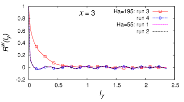
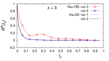
(c)

(d)

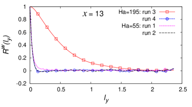
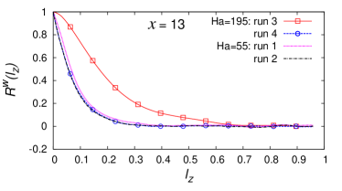
(e)

(f)

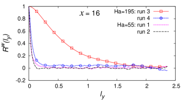
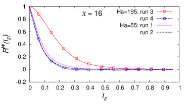
(g)

(h)

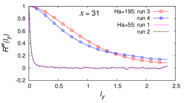
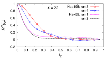
(i)

(j)

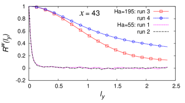
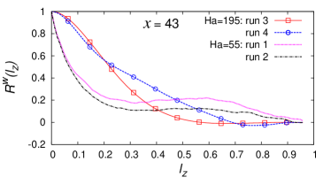
Figure 13: Two-points correlations in the cross-sections at $x=3,13,16,31$ and $43$ for the velocity component $w$ in runs 1-4. Left: correlation coefficients $R^{w}(l_{y})$ versus distance $l_{y}$. Right: correlation coefficients $R^{w}(l_{z})$ versus distance $l_{z}$.

(a)

(b)

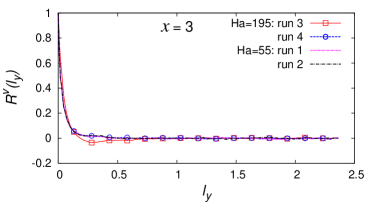
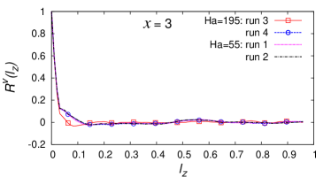
(c)

(d)

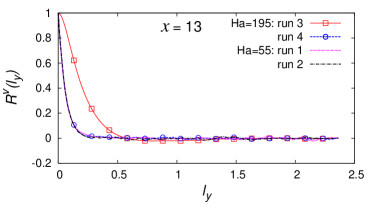
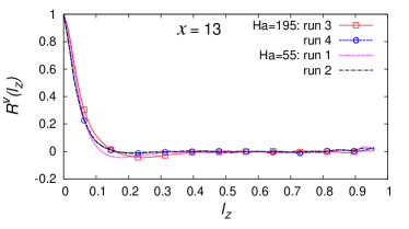
(e)

(f)

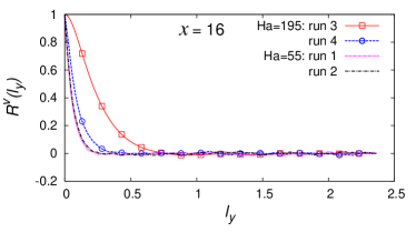
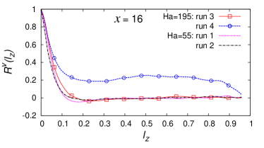
(g)

(h)

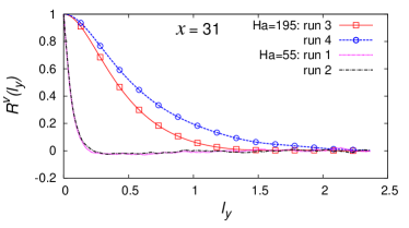
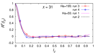
(i)

(j)

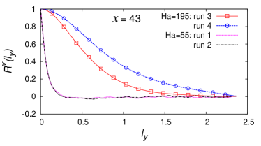
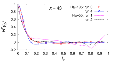
Figure 14: Two-points correlations in the cross-sections at $x=3,13,16,31$ and $43$ for the velocity component $v$ in runs 1-4. Left: correlation coefficients $R^{v}(l_{y})$ versus distance $l_{y}$. Right: correlation coefficients $R^{v}(l_{z})$ versus distance $l_{z}$.

$x=13$              $u$

$v$                                  $w$

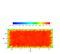
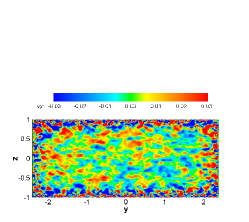
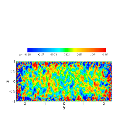
$x=14.5$             $u$

$v$                                  $w$

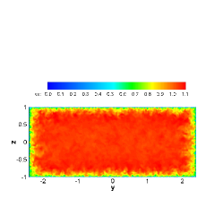
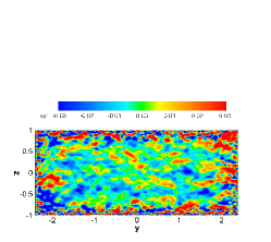
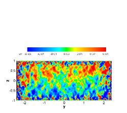
$x=16$              $u$

$v$                                  $w$

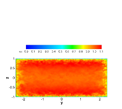
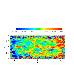
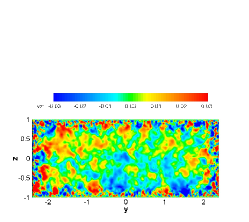
Figure 15: Transformation of the flow in the run 4 at the entrance into the strong magnetic field zone. Instantaneous distributions of the three velocity components at $x=13$, $14.5$ and $16$ are shown.

The two-point correlation functions obtained for the transverse velocity components $w$ and $v$ in the simulations 1-4 are shown in figures 13 and 14. Long-range correlations remain weak in the flows 1 and 2 during the entire decay and that there is practically no difference between the two curves. This confirms the essentially three-dimensional small-scale structure of turbulence in these flows.

The development of of strong correlations along the magnetic field in the flows 3 and 4 is consistent with the results of earlier simulations and theoretical models (see e.g. Moffatt, 1967; Davidson, 1997; Zikanov & Thess, 1998; Krasnov et al., 2008; Burattini et al., 2010) of transformation of turbulent flow under the impact of a strong magnetic field. While the growth of the typical scale of the turbulent structures in the field direction is always stronger and the only one caused directly by the Joule dissipation, the growth of the typical transverse size is caused by the enlargement of the quasi-two-dimensional vortices.

The results obtained for the correlation coefficient $R^{v}$ in flow 4 at $x=16$ (see figure 14f) may appear surprising. The flow has nearly constant significant correlations ($R^{v}\approx 0.2$) over almost the entire duct width. This is not observed for any other computed correlation coefficient in any other cross-section. The reason for this behavior is illustrated in figure 15. From $x=13$ to $x=16$, the streamwise velocity $u$ changes its profile in the way typical for a duct flow entering a strong magnetic field (see e.g. Andreev et al., 2006, for a discussion of the flow transformation). Along the $y$-axis parallel to the magnetic field, the Hartmann profile with nearly uniform velocity in the core and thin Hartmann boundary layers develops. Along the $z$-axis, the profiles acquires the typical M-shape. The redistribution of the streamwise velocity is accompanied by a non-zero mean flow toward the walls at $y=\pm 1$ (clearly visible in the distribution of $v$ at $x=16$) and in the $z$-direction (visible in the distribution of $w$ at $x=14.5$, i.e. slightly upstream of the beginning of full-strength magnetic field, in agreement with the scenario of formation of the M-shaped profile). The elevated correlation coefficient $R^{v}$ in flow 4 at $x=16$ is caused by the flow in the $y$-direction.

References

- Adams et al. (1999) Adams, J. C., Swarztrauber, P. & Sweet, R. 1999 Efficient fortran subprograms for the solution of separable elliptic partial differential equations. http://www.cisl.ucar.edu/css/software/fishpack/.
- Alemany et al. (1979) Alemany, A., Moreau, R., Sulem, P. L. & Frisch, U. 1979 Influence of an external magnetic field on homogeneous MHD turbulence. J. Mec. 18, 277–313.
- Andreev et al. (2006) Andreev, O., Kolesnikov, Y. & Thess, A. 2006 Experimental study of liquid metal channel flow under the influence of a nonuniform magnetic field. Physics of Fluids 18 (6), 65108.
- Boeck et al. (2008) Boeck, T., Krasnov, D., Thess, A. & Zikanov, O. 2008 Large-scale intermittency of liquid-metal channel flow in a magnetic field. Phys. Rev. Lett. 101, 244501.
- Braiden et al. (2016) Braiden, L., Krasnov, D., Molokov, S., Boeck, T. & Bühler, L. 2016 Transition to turbulence in Hunt’s flow in a moderate magnetic field. Europhys. Lett. 115 (4), 084501.
- Branover (1978) Branover, H. 1978 Magnetohydrodynamic Flow in Ducts. New York: Wiley, Hoboken NJ.
- Branover et al. (1970) Branover, H. H., Gelfgat, Y. M., Kit, L. G. & Platnieks, I. A. 1970 Effect of a transverse magnetic field on the intensity profiles of turbulent velocity fluctuations in a channel of rectangular cross section. Magnetohydrodynamics pp. 336–342.
- Brethouwer et al. (2012) Brethouwer, G., Duguet, Y. & Schlatter, P. 2012 Turbulent-laminar coexistence in wall flows with Coriolis, buoyancy or Lorentz forces. J. Fluid Mech. 704, 137–172.
- Burattini et al. (2010) Burattini, P., Zikanov, O. & Knaepen, B. 2010 Decay of magnetohydrodynamic turbulence at low magnetic Reynolds number. J. Fluid Mech. 657, 502–538.
- Davidson (1997) Davidson, P. 1997 The role of angular momentum in the magnetic damping of turbulence. J. Fluid Mech. 336, 123–150.
- Davidson (2016) Davidson, P. A. 2016 Introduction to magnetohydrodynamics. Cambridge University Press.
- Favier et al. (2010) Favier, B., Godeferd, F. S., Cambon, C. & Delache, A. 2010 On the two-dimensionalization of quasistatic magnetohydrodynamic turbulence. Phys. Fluids 22 (7), 75104.
- Favier et al. (2011) Favier, B., Godeferd, F. S., Cambon, C., Delache, A. & Bos, W. J. T. 2011 Quasi-static magnetohydrodynamic turbulence at high Reynolds number. J. Fluid Mech. 681, 434–461.
- Kim & Choi (2009) Kim, J. & Choi, H. 2009 Large eddy simulation of a circular jet: effect of inflow conditions on the near field. J. Fluid Mech. 620, 383.
- Kljukin & Kolesnikov (1989) Kljukin, A. A. & Kolesnikov, J. B. 1989 MHD turbulence decay behind spatial grids. In Liquid Metal Magnetohydrodynamics, pp. 153–159. Springer.
- Knaepen et al. (2004) Knaepen, B., Kassinos, S. & Carati, D. 2004 Magnetohydrodynamic turbulence at moderate magnetic Reynolds number. J. Fluid Mech. 513, 199–220.
- Knaepen & Moin (2004) Knaepen, B. & Moin, P. 2004 Large-eddy simulation of conductive flows at low magnetic Reynolds number. Phys. Fluids 16 (5), 1255.
- Kobayashi et al. (2012) Kobayashi, H., Shionoya, H. & Okuno, Y. 2012 Turbulent duct flows in a liquid metal magnetohydrodynamic power generator. J. Fluid Mech. 713, 243–270.
- Kolesnikov & Tsinober (1974) Kolesnikov, Y. B. & Tsinober, A. B. 1974 Experimental investigation of two-dimensional turbulence behind a grid. Fluid Dynamics 9 (4), 621–624.
- Krasnov et al. (2013) Krasnov, D., Thess, A., Boeck, T., Zhao, Y. & Zikanov, O. 2013 Patterned turbulence in liquid metal flow: Computational reconstruction of the Hartmann experiment. Phys. Rev. Lett. 110, 084501.
- Krasnov et al. (2011) Krasnov, D., Zikanov, O. & Boeck, T. 2011 Comparative study of finite difference approaches to simulation of magnetohydrodynamic turbulence at low magnetic Reynolds number. Comp. Fluids 50, 46–59.
- Krasnov et al. (2008) Krasnov, D., Zikanov, O., Schumacher, J. & Boeck, T. 2008 Magnetohydrodynamic turbulence in a channel with spanwise magnetic field. Phys. Fluids 20 (9), 095105.
- Krasnov et al. (2012) Krasnov, D. S., Zikanov, O. & Boeck, T. 2012 Numerical study of magnetohydrodynamic duct flow at high Reynolds and Hartmann numbers. J. Fluid Mech. 704, 421–446.
- Li & Zikanov (2013) Li, Y. & Zikanov, O. 2013 Laminar pipe flow at the entrance into transverse magnetic field. Fusion Eng. Des. 88 (4), 195–201.
- Moffatt (1967) Moffatt, K. 1967 On the suppression of turbulence by a uniform magnetic field. J. Fluid Mech. 23, 571–592.
- Müller & Bühler (2001) Müller, U. & Bühler, L. 2001 Magnetohydrodynamics in channels and containers. Springer, Berlin.
- Pothérat & Klein (2014) Pothérat, A. & Klein, R. 2014 Why, how and when mhd turbulence at low becomes three-dimensional. J. Fluid Mech. 761, 168–205.
- Pothérat & Klein (2017) Pothérat, A. & Klein, R. 2017 Do magnetic fields enhance turbulence at low magnetic reynolds number? Phys. Rev. Fluids 2 (6), 063702.
- Reddy & Verma (2014) Reddy, K. S. & Verma, M. K. 2014 Strong anisotropy in quasi-static magnetohydrodynamic turbulence for high interaction parameters. Phys. Fluids 26 (2), 025109.
- Schumann (1976) Schumann, U. 1976 Numerical simulation of the transition from three- to two-dimensional turbulence under a uniform magnetic field. J. Fluid Mech. 74, 31–58.
- Sommeria & Moreau (1982) Sommeria, J. & Moreau, R. 1982 Why, how and when MHD-turbulence becomes two-dimensional. J. Fluid Mech. 118, 507–518.
- Sukoriansky et al. (1986) Sukoriansky, S., Zilberman, I. & Branover, H. 1986 Experimental studies of turbulence in mercury flows with transverse magnetic fields. Experiments in Fluids 4 (1), 11–16.
- Thess & Zikanov (2007) Thess, A. & Zikanov, O. 2007 Transition from two-dimensional to three-dimensional magnetohydrodynamic turbulence. J. Fluid Mech. 579, 383–412.
- Verma (2017) Verma, M. K. 2017 Anisotropy in quasi-static magnetohydrodynamic turbulence. Rep. Progr. Phys. 80 (8), 087001.
- Verma & Reddy (2015) Verma, M. K. & Reddy, K. S. 2015 Modeling quasi-static magnetohydrodynamic turbulence with variable energy flux. Phys. Fluids 27 (2), 025114.
- Vorobev & Zikanov (2007) Vorobev, A. & Zikanov, O. 2007 Smagorinsky constant in LES modeling of anisotropic MHD turbulence. Theor. Comp. Fluid Dyn. 22 (3-4), 317–325.
- Vorobev et al. (2005) Vorobev, A., Zikanov, O., Davidson, P. A. & Knaepen, B. 2005 Anisotropy of magnetohydrodynamic turbulence at low magnetic Reynolds number. Phys. Fluids 17 (12), 125105.
- Voronchikhin et al. (1985) Voronchikhin, V. A., Genin, L. G., Levin, V. B. & Sviridov, V. G. 1985 Experimental investigation of grid turbulence decay in a uniform magnetic field. Magnetohydrodynamics (4), 131–134.
- Votsish & Kolesnikov (1976a) Votsish, A. D. & Kolesnikov, Y. B. 1976a Spatial correlation and vorticity in two-dimensional homogeneous turbulence. Magnetohydrodynamics pp. 25–28.
- Votsish & Kolesnikov (1976b) Votsish, A. D. & Kolesnikov, Y. B. 1976b Study of transition from three-dimensional to two-dimensional turbulence in a magnetic field. Magnetohydrodynamics p. 141.
- Votyakov et al. (2009) Votyakov, E. V., Kassinos, S. C. & Albets-Chico, X. 2009 Analytic models of heterogenous magnetic fields for liquid metal flow simulations. Theor. Comp. Fluid Dyn. 23, 571–578.
- Zikanov et al. (2014a) Zikanov, O., Krasnov, D., Boeck, T., Thess, A. & Rossi, M. 2014a Laminar-Turbulent Transition in Magnetohydrodynamic Duct, Pipe, and Channel Flows. Appl. Mech. Rev. 66 (3), 030802.
- Zikanov et al. (2014b) Zikanov, O., Krasnov, D., Li, Y., Boeck, T. & Thess, A. 2014b Patterned turbulence in spatially evolving magnetohydrodynamic tube flows. Theor. Comp. Fluid Dyn. 28 (3), 319–334.
- Zikanov et al. (2013) Zikanov, O., Listratov, Y. & Sviridov, V. G. 2013 Natural convection in horizontal pipe flow with strong transverse magnetic field. J. Fluid Mech. 720, 486–516.
- Zikanov & Thess (1998) Zikanov, O. & Thess, A. 1998 Direct numerical simulation of forced MHD turbulence at low magnetic Reynolds number. J. Fluid Mech. 358, 299–333.