Adaptive Tensegrity Locomotion on Rough Terrain via Reinforcement Learning

Abstract

The dynamical properties of tensegrity robots give them appealing ruggedness and adaptability, but present major challenges with respect to locomotion control. Due to high-dimensionality and complex contact responses, data-driven approaches are apt for producing viable feedback policies. Guided Policy Search (GPS), a sample-efficient and model-free hybrid framework for optimization and reinforcement learning, has recently been used to produce periodic locomotion for a spherical 6-bar tensegrity robot on flat or slightly varied surfaces. This work provides an extension to non-periodic locomotion and achieves rough terrain traversal, which requires more broadly varied, adaptive, and non-periodic rover behavior. The contribution alters the control optimization step of GPS, which locally fits and exploits surrogate models of the dynamics, and employs the existing supervised learning step. The proposed solution incorporates new processes to ensure effective local modeling despite the disorganized nature of sample data in rough terrain locomotion. Demonstrations in simulation reveal that the resulting controller sustains the highly adaptive behavior necessary to reliably traverse rough terrain.

I Introduction

Tensegrity structures consist of rods suspended in a network of elastic cables, so that all elements can freely pivot at the “nodes” where they are connected. Force responses then occur as a compliant reconfiguration of the structure, avoiding localized accumulation of stresses and requiring less total material weight to withstand a given load. When granted the ability to change the lengths of their elements, tensegrities can be made into robots that exhibit appealing ruggedness and adaptability to rough terrain, such as NASA’s 6-bar tensegrity rover, SUPERball [1], shown in Fig. 1. The same dynamical properties, however, also make tensegrity locomotion control a hard and unintuitive problem [2, 3].

Deformation-based locomotion of tensegrities generally relies upon the geometric relationship between the supporting base polygon and the center-of-mass (CoM). By deforming into a statically unstable configuration, a “flop” forward onto an adjacent triangle can be induced [4]. Hand-engineered methods may achieve this by actuating just one or two elements, as has recently been demonstrated in both software and hardware for ascending uniform inclines as steep as $26^{\circ}$ [5]. Given a model or database of the relationship between cable lengths and vehicle shape, many-cable solutions can be discovered by search or optimization [6, 7, 8], opening the door to more precise or adaptive behaviors.

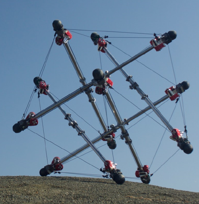
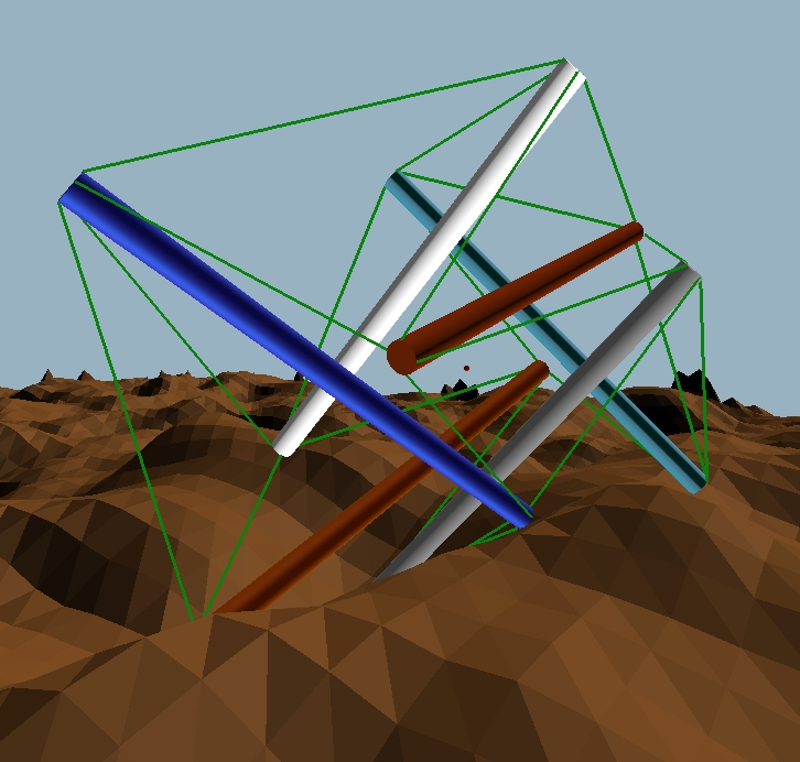
Figure 1: Left: hardware prototype of SUPERball version 2 at NASA Ames. Right: Simulated behavior exiting a deep pit in rough terrain.

I-A Related Work

Dynamic tensegrity locomotion involves numerous complex factors, such as a varying contact interface with the ground, that complicate the use of model-based control. Sampling-based motion planning, which has been used for quasi-static deformation [9], can also be applied to design kinodynamic paths that demonstrate the aptitude of tensegrities on complex terrain [10]. The open-loop nature of this approach, however, is inevitably fragile to errors, and it is too computationally costly to be re-applied online.

This has motivated numerous investigations using data-driven control methods, such as Central Pattern Generators (CPGs) [11, 12], evolutionary algorithms [13, 14], and reinforcement learning [15]. CPGs can provide robust locomotive gaits, but may limit the vehicle’s ability to proactively adapt to the environment with highly expressive shape changes. Evolutionary algorithms have been used to produce sustained locomotion on terrain by a 6-bar tensegrity in simulation [16], but typically require very large datasets.

Reinforcement learning is often also associated with excessive data requirements. Guided Policy Search (GPS) is a hybrid technique that strongly reduces these requirements by exploiting gradient information, but without the need for an apriori system model [17]. GPS has been applied to produce a periodic locomotive gait on the original hardware prototype of SUPERball, which could actuate only half of its tensile members [15]. Similar behavior by a fully-actuated 6-bar tensegrity was also achieved in simulation on a surface with height variations of a few percent of a bar length [18].

A commonality of prior controllers for 6-bar tensegrity locomotion [5, 16, 15, 18] is the regularity and periodicity of their behavior. This could limit the adaptiveness of the vehicle to increasingly unstructured environments, where contact geometry becomes strongly perturbed and the few discrete options for CoM motion may coincide with obstacles. For the two studies using GPS [15, 18], this limitation is related to the method’s requirement for sample data to be organized into local neighborhoods that correspond to linear time-varying surrogate models of the dynamics.

This general limitation of GPS has been identified and partially addressed by “Reset-Free” GPS, which utilizes clustering to provide post-hoc localization of sample data [19]. That modification, however, targeted transient manipulation tasks and does not address the timing variations involved in sustained non-periodic behaviors, such as adaptive locomotion. Combined with other limitations, this has motivated recent work by the current authors in adapting the GPS pipeline to enable any-axis locomotion of a 6-bar tensegrity on a flat terrain, such that the CoM can follow arbitrary paths relative to the contact geometry [20]. The scope of that experimentally-focused investigation, however, was restricted to exploring the nature of any-axis motion on the plane, did not address the case of rough terrain, and did not permit the detailed description or evaluation of the algorithmic components that allow any-axis behavior to emerge.

I-B Contributions and Outline

This paper extends the line of work on adapting and employing the GPS reinforcement learning framework for any-axis planar locomotion with a tensegrity robot [20], as an example application domain that involves complex dynamics and compliance. Sec. II outlines GPS and 6-bar tensegrity traits, along with a scheme for symmetry exploitation that mitigates growth in sample complexity relative to that of the more narrow-scope controllers in related prior work [15, 18]. The applied modifications in the GPS pipeline are described in Sec. III including dimensionality reduction of the surrogate models, an alternate post-hoc localization scheme relative to “Reset-Free” GPS [19], and an additional localization step introduced relative to prior work by the authors [20].

Experimental details are provided in Sec. IV, including description of a terrain environment of comparable or greater difficulty than previous extremes [16, 5]. Sec. V demonstrates a controller that successfully traverses this environment, while also exhibiting any-axis characteristics. The method will be referred to as T6-GPS, to acknowledge its significant tailoring to the nature of 6-bar tensegrities. Nevertheless, the discussion of Sec. VI will address the more general lessons of this investigation that can impact the deployment of reinforcement learning pipelines, such as GPS, to other highly complex and dynamical systems.

II Background

Let $\mathbf{x}^{\prime}=\phi\left(\mathbf{x},\mathbf{u}\right)$ describe the discrete-time, nonlinear system dynamics as a function of the state $x$ and controls $u$. With observation $\mathbf{y}\left(\mathbf{x}\right)$, define a control policy $\mathbf{u}=\pi_{\theta}\left(\mathbf{y}\right)$ governed by a parameter vector $\theta$. The closed-loop dynamics are then $\mathbf{x}^{\prime}=\phi\left(\mathbf{x},\pi_{\theta}\left(\mathbf{y}\left(\mathbf{x}\right)\right)\right)$. Using the combined state/action vector $\mathbf{r}=\left[\begin{array}[]{cc}\mathbf{x}^{T}&\mathbf{u}^{T}\end{array}\right]^{T}$, a trajectory $\tau=\left[\begin{array}[]{cccc}\mathbf{r}_{0},\mathbf{r}_{1},\ldots,\mathbf{r}_{T-1}\end{array}\right]$ is the length-$T$ sequence generated by $\phi$ and $\pi_{\theta}$ for an initial state $\mathbf{x}_{0}$. Finally, let the running cost $l\left(\mathbf{r}\right)$ be the performance metric for any given time step of controlled dynamics.

II-A Guided Policy Search

The term Policy Search refers to a class of algorithms that calibrate a parameterized control policy by searching the space of parameter values $\theta$. Under a dataset consisting of $N$ trajectories of length $T$, this corresponds to the objective

$$\theta^{*}=\texttt{argmin}\,\Sigma_{i=0}^{N-1}\Sigma_{t=0}^{T-1}l\left(\tau_{i}\left(t\right)\right).$$ (1)

As the complexity of the control policy architecture increases, evolutionary algorithms and other black-box optimization approaches to discover $\theta^{*}$ require significant amounts of sample data. Guided Policy Search (GPS) is a technique designed to train an artificial neural network representation of $\pi_{\theta}$ with only moderate sample complexity and no requirement of an explicit, differentiable dynamics model [17]. The method combines control optimization (the C-step) and supervised learning (the S-step).

Key to the sample efficiency of GPS is its exploitation of system gradient information within the C-step. In the absence of an apriori model, gradients of $\phi$ and $\pi_{\theta}$ with respect to the state-action $\mathbf{r}$ are approximated by fitting linear time-varying surrogate models $f$ and $p$ to the sample data:

$$\mathbf{x}^{\prime}=f\left(t,\mathbf{r}\right) =F(t)\mathbf{r}+\mathbf{f}(t)$$ (2)

$$\mathbf{u}=p\left(t,\mathbf{x}\right) =P(t)\mathbf{x}+\mathbf{p}(t)\vspace{-.15in}$$ (3)

With the assumption that $l\left(\mathbf{r}\right)$ is analytic, it is then possible to compute an improved local policy $p^{*}(t,\mathbf{x})$ via the iterative Linear Quadratic Gaussian (iLQG) [21] using differentiable $l(t,\mathbf{r})$ and $f(t,\mathbf{r})$. Applying this policy to the original state sequence produces variationally improved actions $\mathbf{u}^{*}$.

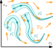
Figure 2: The “S-step” of GPS encodes multiple local controllers $p_{j}^{*}$ into one global controller $\pi_{\theta}$.

Because both $\phi$ and $\pi$ are nonlinear, their surrogate models have only limited local validity. Several of these models $m_{j}=\left(f_{j},p_{j}\right)$ may then be necessary for improving feedback actions for a large region of the state space. The S-step consists of using a globally accumulated set of observations and corresponding locally improved actions, $D=\left\{\mathbf{y},\mathbf{u}^{*}\right\}$, for supervised training of the policy, i.e., learning $\theta$. Fig. 2 illustrates this step as the matching of the global policy field $\pi\left(\mathbf{x}\right)$ to a set of local policies $p_{j}^{*}$ that funnel nearby states along a targeted path.

1 $D\leftarrow\emptyset$

2 foreach $\mathbf{x}_{0}\in\mathcal{X}_{0}$ do

3       $\mathcal{T}\leftarrow$ RunSamples($\mathbf{x}_{0},\theta_{i-1},N$)

4       $m\leftarrow$ FitLocalModel($\mathcal{T}$)

5       $\mathcal{T}^{*}\leftarrow$ LQGBackwardPass($\mathcal{T},m,l\left(\mathbf{r}\right)$)

6       $D\leftarrow D\;\cup$ GetObservationActionPairs($\mathcal{T}^{*}$)

7      

8 end foreach

9$\theta_{i}\leftarrow$ SupervisedLearning($\theta_{i-1},D$)

Algorithm 1 GPS Iteration

Algorithm 1 outlines the high-level procedure for one iteration of GPS. For each $x_{0}$ of a set of initial conditions $\mathcal{X}_{0}$, the previous policy $\theta_{i-1}$ is executed $N$ times to generate sample trajectories $\tau_{k}\in\mathcal{T}$. The time varying local model $m$ is then fit and used to conduct a backward pass, updating each $\mathbf{u}$ to $\mathbf{u}^{*}$. These are paired with corresponding observations in the dataset $D=\left\{\mathbf{y},\mathbf{u}^{*}\right\}$ to supervise learning of $\theta$.

Convergence is aided by augmenting the cost function with a KL-divergence term, $l^{\prime}\left(\mathbf{r},p\right)=l\left(\mathbf{r}\right)+cKL\left(p^{*}||p\right)$. With weight $c$, this penalizes the difference between the policy $p^{*}$, which improves the cost, and the surrogate model $p$ of the policy that generated the original trajectory.

II-B System Description

SUPERball is composed of 6 rigid bars, 1.94m long, that are isolated in compression within a network of 24 actuated cables in tension. This connectivity scheme is illustrated in Fig. 3, which also highlights the 8 exterior triangular faces defined by three cables ($\Delta$ type) While these triangles never share a common edge, the remaining 12 triangles ($\Lambda$ type) occur in pairs that share a “virtual” edge without a cable.

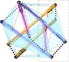
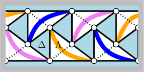
Figure 3: Topology of a 6-bar icosahedral tensegrity shown in 3D and 2D, using a cutting section shown in gray. Solid lines indicate cables; dotted lines are virtual edges. $\Delta$ type triangles are shaded blue, $\Lambda$ unshaded.

The state $\mathbf{x}$ consists of the 6-DoF rigid body state of each bar along with the rest length of each cable, which may differ from its actual length due to elastic deformation. The control input $\mathbf{u}$ is the vector of desired cable rest lengths, while a separate control layer attempts to satisfy these specifications via motorized spools. The simulation testbed representing $\phi\left(\mathbf{r}\right)$ is the NASA Tensegrity Robotics Toolkit (NTRT) [22].

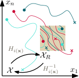
Figure 4: Symmetry reduction of the state-action space volume.

In its neutral stance, SUPERball is a pseudo-icosahedron with 24th-order symmetry. Although deformation breaks spatial symmetry, each symmetric transformation can still be related to a permutation of the IDs of elements, which does not alter the vehicle’s dynamics. 24 maps $H_{i}$ can then be defined that combine label permutation with a gravity-preserving orthogonal transformation, such that the intrinsic dynamics of the vehicle are not violated, i.e., $\phi\left(\mathbf{r}\right)=H_{i}^{-1}\phi\left(H_{i}\mathbf{r}\right)$. Symmetry reduction is achieved by defining a rule $i(\mathbf{x})$ such that all states are losslessly mapped into a volume 1/24th as large as the full space [23]. The chosen rule produces one reference frame each for $\Delta$ and $\Lambda$ types of bottom triangles (beneath the CoM) with fixed orientation.

III T6-GPS for Nonperiodic Locomotion

The modified GPS algorithm tailored for 6-bar tensegrities, T6-GPS, is outlined in Fig. 5 and detailed in Algorithm. 2.

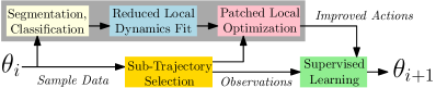
Figure 5: T6-GPS iteration. Components within the gray box utilize dynamics reduction and post-hoc localization.

1 $M,D_{i}\leftarrow\emptyset$

2 $\mathcal{T}\leftarrow$ RunSamples($\mathcal{X}_{0},\theta_{i-1}$)

3 $S\leftarrow$ SegmentSamples($\mathcal{T}$)

4 foreach $\xi\in\Xi$ do

5       $S_{\xi}\leftarrow$ FilterSegments($S,\xi$)

6       $M\leftarrow M\;\cup$ FitLocalModels($S_{\xi}$)

7      

8 end foreach

9foreach $\tilde{\tau}\in$ GetSubTrajectories($\mathcal{T}$) do

10       $\tilde{m}\leftarrow$ PatchModelSeries($\tilde{\tau},M$)

11       $\tilde{\tau}^{*}\leftarrow$ LQGBackwardPass($\tilde{\tau},\tilde{m},l\left(\mathbf{r}\right)$)

12       $D_{i}\leftarrow D_{i}\;\cup$ GetObservationActionPairs($\tilde{\tau}^{*}$)

13      

14 end foreach

15$\theta_{i}\leftarrow$ SupervisedLearning($\theta_{i-1},D_{i}$)

Algorithm 2 T6-GPS Iteration

While Alg. 1 conducted repeated sampling of specific initial conditions, which previous work [15, 18] used to ensure periodic behavior, Alg. 2 does not enforce any apriori structure on the sample set. Instead, post-hoc localization is conducted in lines 3-7, which is important for accommodating any-axis and terrain-adaptive motion that does not routinely repeat identical movements. This process, shown in the upper track of Fig. 5, begins with coarse localization through segment classification (lines 3-5, detailed in Sec. III-A). Further localization steps are then taken in line 6, which corresponds to Sec. III-B–III-D. Lines 8-9 associate the localized data back to original samples to allow completion of the C-step, described in Sec. III-E. Finally, lines 11-13 represent standard data accumulation and policy training.

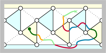
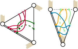
(a) (b) (c)

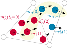
Figure 6: (a) segmentation of a single trajectory based upon CoM crossings over different bottom support triangles; (b) classifying symmetry-reduced segments based on bottom triangle type and start/end edge relationships; (c) fitting one or more surrogate models per time step per segment class.

III-A Segmentation and Classification

The first stage of post-hoc data localization breaks each trajectory into several segments $s=\tau\left(a\leq t<b\right)=\left[\begin{array}[]{cccc}\mathbf{r}_{a},\mathbf{r}_{a+1},\ldots,\mathbf{r}_{b-1}\end{array}\right]$, which are appropriate for a linear time-varying model. A natural criterion for this arises from the imposed scheme for symmetry reduction into two bottom-triangle reference frames: segments are cut when the bottom triangle ID changes, as illustrated in Fig. 6(a). Segments are then classified via Boolean-valued functions $\xi\left(s\right)$ such that FilterSegments returns the segment set $\left\{s\in S\;|\;\xi\left(s\right)\right\}$. Fig. 6(b) illustrates segments within the symmetry-reduced space, colored based on their class.

III-B Local Models - Time Warping

As is apparent in Fig. 6(b), two segments may have similar characteristics while nonetheless occurring at different rates or durations. Within FitLocalModels in Alg. 2, time warping is used to accumulate data points along a fixed-length time series $t_{\xi}=0,1,\ldots,T_{\xi}-1$. Each $k$’th segment uses a time mapping $\tilde{t}_{\xi k}\in\mathbb{N}^{T_{\xi}}$ such that $s_{k}\left(\tilde{t}_{\xi k}\left(t_{\xi}\right)\right)$ returns the point from segment $k$ to be associated with the $t_{\xi}$-th time-step of the class. Although more complex methods were considered [24], it was found that a simple “uniform stretch” strategy functioned sufficiently, where for example a point halfway along a segment aligns to the time $T_{\xi}/2$.

III-C Local Models - Dynamics Reduction

The symmetry-based reduction described in Sec. II-B shrinks the volume of state space that must be covered by surrogate models and the global policy. A further reduction, illustrated by the gray box in Fig. 5, is applied to decrease the state dimension accounted for in local fitting and optimization. A linear map $L:\mathbf{x}\rightarrow\bar{\mathbf{x}}$ is applied within FitLocalModels such that $m$ expresses $\bar{\mathbf{x}}=f\left(t,\bar{\mathbf{r}}\right)$ and $\mathbf{u}=p\left(t,\bar{\mathbf{x}}\right)$, where $\bar{\mathbf{r}}=\left[\begin{array}[]{cc}\bar{\mathbf{x}}^{T}&\mathbf{u}^{T}\end{array}\right]^{T}$. The purpose is to capture only the primary dynamical influences, so that the variational relationship between the control input and the resulting cost is coarsely but robustly approximated. Selection of $L$ must permit the evaluation $l\left(\bar{\mathbf{x}}\right)$, i.e., observability of the cost.

III-D Local Models - Multi-Modal Fitting

The preceding steps produce one aligned series of reduced state-action sets for each class: $\left[\left\{\bar{\mathbf{r}}_{0}\right\},\left\{\bar{\mathbf{r}}_{1}\right\},\ldots,\left\{\bar{\mathbf{r}}_{T_{\xi}-1}\right\}\right]_{\xi}$. The next step is to produce multiple linear models per step $t_{\xi}$. The function recursively applies RANSAC linear regression to produce models $m^{h}(t)$ such that the $h$’th mode is fit using the outliers of the $h{-}1$’th mode. Outliers are designated based upon a residual threshold equal to one standard deviation of the dataset. The hypothesis is that this may account for different contact conditions between similarly shaped states, while remaining less computationally intensive than fitting Gaussian mixtures.

III-E Sub-Trajectory Backward Pass

Optimization requires dynamics gradients, provided from the set $M$ of surrogate models, and cost gradients, obtainable analytically for each trajectory. The backward pass horizon is moderated by dividing each trajectory into sub-trajectories $\tilde{\tau}$, which are essentially longer segments, in GetSubTrajectories of Alg. 2. This process keeps the horizon short enough to avoid excessive accumulation of linearization error, but long enough to smooth out behavior across transitions.

Figure 7 illustrates the relationship between segments and sub-trajectories, along with the association of each point to a surrogate model $m^{h}_{\xi}(t)$. Individual models are patched together by PatchModelSeries for use in the BackwardPass, which returns $\tilde{\tau}^{*}$ with updated actions $\mathbf{u}^{*}(t)=p^{*}\left(t,\mathbf{x}(t)\right)$.

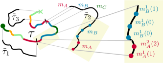
Figure 7: A single trajectory $\tau$ is broken into multiple subtrajectories $\tilde{\tau}$ (left). Each point on a subtrajectory is associated with a surrogate model $m$ via segment classification (center), time warping and modality (right).

IV Experiment Setup

IV-A Scenario

On each iteration of T6-GPS, $N=300$ samples are executed for $T=250$ time steps each. This corresponds to 25 seconds of robot behavior under the applied 10Hz sampling frequency. The initial state set $\mathcal{X}_{0}$ was generated to randomize the vehicle’s location, orientation, and shape.

The rough terrain environment utilized is pictured in 3D in Figs. 1 and 10 and as a contour map in Fig. 9. The average slope of individual facets is $38^{\circ}$ with standard deviation $16^{\circ}$. Hills and troughs exist on length scales similar to the size of SUPERball, with maximal height variations of 1.55m, about 80% of one bar length, which are quite difficult to traverse.

The objective of each trial is to move the CoM through a sequence of five randomly placed waypoints, which are half the diameter of the vehicle. If a waypoint is not reached within five seconds, the next one is activated in order to prevent excessive time spent in stuck states. With $\hat{\mathbf{g}}$ as the direction of the next waypoint, a simple quadratic cost is defined in terms of center-of-mass velocity:

$$l\left(\bar{\mathbf{r}}\right) =\left(\mathbf{v}_{CoM}\left(\bar{\mathbf{x}}\right)-v^{*}\hat{\mathbf{g}}\right)^{T}W\left(\mathbf{v}_{CoM}\left(\bar{\mathbf{x}}\right)-v^{*}\hat{\mathbf{g}}\right)$$ (4)

where the weight matrix $W$ penalizes both ground-plane components equally and de-weights the vertical. A target velocity $v^{*}=0.8$m/s was chosen, which is faster than what can be achieved uphill, but slower than tumbling downhill.

IV-B Segment Classes

Classification functions $\xi\left(s\right)$ evaluate the type of a given trajectory segment according to multiple criteria:

1) The category of the bottom triangle, i.e., $\Delta$ or $\Lambda$, which represent fundamentally different configurations.

2) The type of edge crossed upon entering a support triangle and the type of edge crossed upon exiting it. For $\Delta$ triangles, the edge handedness influences the classification. By reasoning about the start/end edge relationship of a segment path, relatively similar velocity values are achieved per class. This criterion also ensures the same type of final dynamics step, which transfers the state to the next frame; see Fig. 6(c).

3) Distinguishing complete segments from “partial” segments, where either the beginning or ending of the segment is not associated with an edge crossing. This occurs for the first and last segments of each sample trajectory as well as for “truncated” segments, which represent the first portion of long segments where the vehicle becomes stuck rather than reaching its next transition within a reasonable time frame. Classifying truncated segments allows the algorithm to fit accurate surrogate models for improving actions that previously failed to maintain motion of the platform.

Fig. 6(b) visualizes some of the segment classes over $\Delta$ and $\Lambda$ support triangles with different colors and line types.

IV-C Dynamics and Observation Spaces

Several definitions of the reduced state $\bar{\mathbf{x}}$ were evaluated. Each option included the $\mathbf{v}_{CoM}$ to ensure compatibility with the gradient of the cost of Eq. 4 during the backward pass. Remaining contents were drawn from different categories of full state variables: (1) the CoM-relative positions of the lower six nodes, giving static stability and contact information; (2) CoM-relative positions of all 12 nodes, providing shape information; (3) the cable rest lengths, which express tension if the shape is known; and (4) velocities of the nodes.

As outlined in Sec. II-B, the neural net input layer accepts only symmetry-reduced sensor data. It is assumed that the ID of the bottom triangle can be classified from raw sensor data, as is implemented on hardware [25]. The previous and current ID are then used to determine the index of the symmetry reduction transformation $H_{i}$ that expresses observations within the appropriate reference frame. The input layer is then provided with (1) a Boolean indicating $\Delta$ or $\Lambda$ bottom triangle, (2) the rest length for each of the 24 strings, (3) the 3D angular velocity vector of each of the six bars, (4) the target direction $\hat{\mathbf{g}}$ expressed as an angle on the ground plane, and (5) the “track” ground plane angle giving the CoM velocity direction. The neural net itself is a simple fully-connected network with 3 hidden layers and 256 neurons per layer. Finally, the output cable lengths $\mathbf{u}$ are relabeled for use with the actual state via $H_{i}^{-1}$ as in Fig. 4.

V Results

V-A Flat Ground - Data Requirements vs. Standard GPS

Due to fundamental differences between periodic and nonperiodic controllers, direct comparison of T6-GPS to previous approaches [15, 18] is not straightforward. As a coarse comparison point, this work attempts to produce any-axis CoM movement on flat ground without the use of post-hoc data localization or symmetry reduction. This is to evaluate data requirements of standard GPS versus T6-GPS.

Beginning at rest upon a particular $\Delta$ triangle with a fixed orientation, the commanded direction of motion is discretized into $J=36$ values, corresponding to the set of local models $m_{j}$. For each direction, $N=50$ samples of equal length $T=16$ are collected, in keeping with the standard GPS framework of Algorithm 1. After $I=10$ GPS iterations, the controller was able to smoothly move the CoM in commanded directions relative to the initial bottom triangle for one or two transitions — a result of limited scope for a tuned sampling cost of $IJNT=288,000$ total time steps.

This value already compares unfavorably to the $INT=125,000$ required under an early version of T6-GPS for this setup, an increase by a factor of $20$ (the total number of triangles) would be necessary for the standard GPS pipeline to cover all transition cases. Such issues would only be compounded when training for rough terrain, requiring another discretization dimension for $K$ types of terrain features, with accompanying setup effort. These findings motivate the segment classification and time warping components of T6-GPS (III-A and III-B), which naturally complement the use of symmetry reduction, while more naturally and efficiently covering the state space with long sample trajectories.

V-B Rough Terrain - Tuning and Cost Evaluation

The remaining components of T6-GPS are evaluated using the rough terrain environment. The backward pass horizon (Sec. III-E) was not a sensitive parameter. Sub-trajectory lengths $10\leq\tilde{T}\leq 20$ time steps (1 to 2 seconds), which correspond to roughly one or two transitions, provided similar good performance. Results degraded for $\tilde{T}\leq 5$.

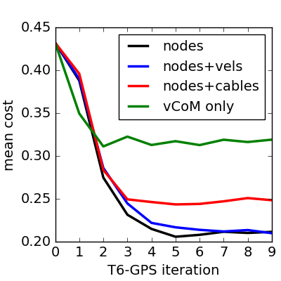
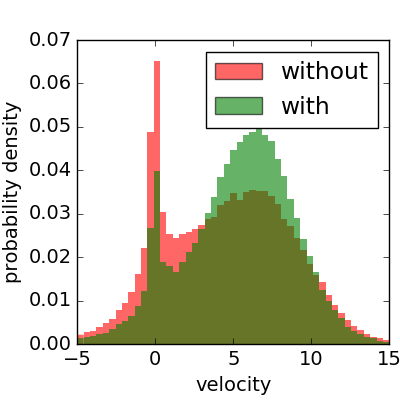
Figure 8: Left: performance of T6-GPS for different surrogate spaces (mean of X runs). Right: velocity distributions without and with multi-modal fits.

Modeling the complete state (node positions, velocities, and cable rest lengths) resulted in memory issues due to excessive dimensionality. Figure 8 plots average sample cost versus iteration count using smaller surrogate model spaces based upon the value types listed in Sec. IV-C. When modeling the cost state alone, $\mathbf{v}_{CoM}$, T6-GPS could merely improve the initial pure-noise policy to a motionless policy. The inclusion of node positions (corresponding to “nodes” in the graph) provided strong performance, converging to a value that will later be shown to correspond to effective locomotion. Additionally including their velocities (“nodes+vels”) marginally increased cost, signaling diminishing returns in the trade off of additional dimensionality incurred for additional information. When instead incorporating the rest lengths of the cables (“nodes+cables”) performance dropped significantly, suggesting that tensional effects would require much narrower localization in order to be approximated effectively. Not shown, omitting the upper six node positions only slightly increased the cost, highlighting the importance of interface geometry over that of the general shape.

Noting that sample costs in Fig. 8 reflect the performance of the previous iteration’s controller, the iteration of convergence is set to $i=5$ and the nodes surrogate space is chosen. A total of $INT=375,000$ sampled time steps were used to produce this controller, with a total runtime of about 1.0 hour on a modern 8-core workstation.

To verify its benefit, multi-modal fitting (III-D) was next disabled, resulting in a cost increase of more than 10%. Fig. 8(b) plots the distribution of the forward speed $\mathbf{v}_{CoM}\cdot\hat{\mathbf{g}}$ with and without this feature, showing that differing rates of stuck states (i.e., states with velocity close to 0) are a major contributor to cost differences. FitLocalModels utilized 4 to 5 modes for the most common segment classes, and 1 or 2 for the least common. Without multiple modes, the optimization step may fail to account for contact differences between otherwise similar states.

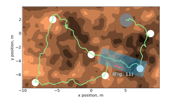
Figure 9: CoM ground-track originating at the gray circle (size of SUPERball) visiting several waypoints (white circles). Darker contours are lower terrain.

V-C Rough Terrain - Locomotive Behavior

Behavior of the top-performing controller is now examined qualitatively. Figure 9 gives a top-down view of a typical CoM path lasting 1.5 minutes (900 steps). The path is generally smooth when motion is level or downhill, with some irregularities or slower progress at uphill portions such as at coordinates (5,-4) and (-3,1). Figure 10 provides snapshots of the (5,-4) hill ascent, which involves two steps up locally steep bumps for a net height gain of more than 2/3 of a bar length. This feature thus has a similar average slope and overall greater roughness relative to the previously attempted terrains  [16] (which maxed out at $18^{\circ}$). Behavior is far less constrained than in uniform slope ascent [5].

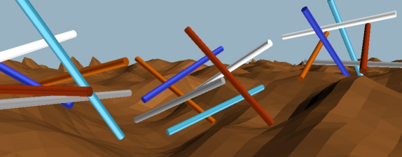
Figure 10: SUPERball traverses to the right across a difficult terrain feature.

A zoomed-in view of the ground track in Fig. 11 provides details about the vehicle’s geometry during this portion of the trial. At the right of the plot, where motion is relatively level or downhill, the nonperiodic nature of the contact pattern reveals the “any-axis” characteristics of the controller. This increased freedom of directionality relative to most prior work [16, 15, 18] could potentially be harnessed by a planner to navigate narrow feasible routes within an especially hazardous landscape.

In the left of Fig 11, overlapping footprints and broad movements of bottom nodes indicate significant slippage of contacts. While the controller nonetheless resolves such features, this friction behavior indicates some limits of the system itself, as also noted in hardware and NTRT [5]. Alteration of the friction coefficient within the NTRT environment did not resolve the slippage, which may require compliant contact modeling for more realistic behavior. This would be in line with the “softball” attachments at the nodes of the latest SUPERball hardware prototype [1].

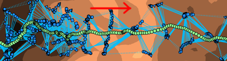
Figure 11: Detailed ground track during hill ascent. Geometry of the triangle below the CoM is shown in blue.

VI Discussion and Future Work

Through the addition and modification of several components within the GPS framework, this work has demonstrated a sample-efficient way of generating a feedback locomotion controller for a simulated 6-bar tensegrity rover on rough terrain. Results showed dynamic, adaptive, and robust nonperiodic behavior for traversing highly nontrivial features involving diverse contact geometries and configurations.

More broadly, this work illustrates that a combination of dimensionality reduction and post-hoc data localization can greatly improve the utility of surrogate models for optimizing sustained adaptive behaviors on high-dimensional robots. While the present implementation of these steps is tailored to 6-bar tensegrities, similar results might be achieved on other platforms via the same principles. For example, localization could be achieved with automated segmentation and aligned cluster analysis, with variational auto-encoding to reduce dimensionality.

By prioritizing the algorithmic discovery of adaptive feedback behaviors, this work fits into the middle of a hierarchy of considerations for useful deployment of mobile tensegrities. The level below is the transfer of such behaviors to hardware, which may involve a reduction of sensor requirements and improved physics models that capture the interaction of cables with convex terrain. One level above is integration with a planning algorithm, which addresses controller limitations, such as occasional stuck states, but should ideally have its role kept simple and lightweight by maximizing controller utility and robustness. These two objectives will steer the direction of future work.

References

- [1] M. Vespignani, J. M. Friesen, V. SunSpiral, and J. Bruce, “Design of superball v2, a compliant tensegrity robot for absorbing large impacts,” in IROS, 2018.
- [2] J. M. Mirats Tur and S. Hernández Juan, “Tensegrity Frameworks: Dynamic Analysis Review and Open Problems,” Mechanism and Machine Theory, vol. 44, no. 1, pp. 1–18, 2009.
- [3] J. Rieffel, F. Valero-Cuevas, and H. Lipson, “Morphological communication: exploiting coupled dynamics in a complex mechanical structure to achieve locomotion,” JRSI, vol. 7, pp. 613–621, 2009.
- [4] M. Shibata, F. Saijyo, and S. Hirai, “Crawling by body deformation of tensegrity structure robots,” in ICRA, 2009.
- [5] L. H. Chen, B. Cera, E. L. Zhu, R. Edmunds, F. Rice, A. Bronars, E. Tang, S. R. Malekshahi, O. Romero, A. K. Agogino, and A. M. Agogino, “Inclined surface locomotion strategies for spherical tensegrity robots,” in 2017 IEEE/RSJ International Conference on Intelligent Robots and Systems (IROS), Sept. 2017, pp. 4976–4981.
- [6] K. Kim, A. K. Agogino, A. Toghyan, D. Moon, L. Taneja, and A. M. Agogino, “Robust learning of tensegrity robot control for locomotion through form-finding,” in IROS, 2015.
- [7] Z. Littlefield, D. Surovik, W. Wang, and K. E. Bekris, “From quasi-static to kinodynamic planning for spherical tensegrity locomotion,” in International Symosium on Robotics Research (ISRR), Puerto Varas, Chile, 12/2017 2017.
- [8] Y. Zhao, S. Zhou, C. Lin, and D. Li, “An efficient locomotion strategy for six-strut tensegrity robots,” in Control & Automation (ICCA), 2017 13th IEEE International Conference on. IEEE, 2017, pp. 413–418.
- [9] J. M. Porta and S. Hernández Juan, “Path planning for active tensegrity structures,” IJSS, vol. 78–79, pp. 47 – 56, 2016. [Online]. Available: http://www.sciencedirect.com/science/article/pii/S0020768315004035
- [10] Z. Littlefield, K. Caluwaerts, J. Bruce, V. SunSpiral, and K. E. Bekris, “Integrating simulated tensegrity models with efficient motion planning for planetary navigation,” in i-SAIRAS, June 2016.
- [11] B. Mirletz, P. Bhandal, R. D. Adams, A. K. Agogino, R. D. Quinn, and V. SunSpiral, “Goal directed CPG based control for high DOF tensegrity spines traversing irregular terrain,” Soft Robotics, 2015.
- [12] C. Rennie and K. E. Bekris, “Discovering a library of rhythmic gaits for spherical tensegrity locomotion,” in IEEE International Conference on Robotics and Automation (ICRA), Brisbane, Australia, 2018.
- [13] A. Iscen, K. Caluwaerts, J. Bruce, A. Agogino, V. SunSpiral, and K. Tumer, “Learning tensegrity locomotion using open-loop control signals and coevolutionary algorithms,” Artificial Life, vol. 21, no. 2, pp. 119–140, May 2015.
- [14] C. Paul, F. J. Valero-Cuevas, and H. Lipson, “Design and control of tensegrity robots for locomotion,” TRO, vol. 22, no. 5, Oct. 2006.
- [15] M. Zhang, X. Geng, J. Bruce, K. Caluwaerts, M. Vespignani, V. SunSpiral, P. Abbeel, and S. Levine, “Deep reinforcement learning for tensegrity robot locomotion,” in 2017 IEEE International Conference on Robotics and Automation (ICRA), May 2017, pp. 634–641.
- [16] A. Iscen, A. Agogino, V. SunSpiral, and K. Tumer, “Flop and roll: Learning robust goal-directed locomotion for a tensegrity robot,” in IROS, 2014, pp. 2236–2243.
- [17] S. Levine and P. Abbeel, “Learning Neural Network Policies with Guided Policy Search under Unknown Dynamics,” in NIPS 27, 2014, pp. 1071–1079.
- [18] J. Luo, R. F. Edmunds, F. Rice, and A. M. Agogino, “Tensegrity robot locomotion under limited sensory inputs via deep reinforcement learning,” in 2018 IEEE International Conference on Robotics and Automation (ICRA), May 2018.
- [19] W. Montgomery, A. Ajay, C. Finn, P. Abbeel, and S. Levine, “Reset-free guided policy search: Efficient deep reinforcement learning with stochastic initial states,” in 2017 IEEE International Conference on Robotics and Automation (ICRA), May 2017, pp. 3373–3380.
- [20] D. Surovik, J. Bruce, K. Wang, M. Vespignani, and K. E. Bekris, “Any-axis tensegrity rolling via symmetry-reduced reinforcement learning,” in 2018 International Symposium on Experimental Robotics, Nov. 2018.
- [21] Y. Tassa, T. Erez, and E. Todorov, “Synthesis and stabilization of complex behaviors through online trajectory optimization,” in 2012 IEEE/RSJ International Conference on Intelligent Robots and Systems, Oct. 2012, pp. 4906–4913.
- [22] “NASA Tensegrity Robotics Toolkit,” ti.arc.nasa.gov/tech/asr/intelligent-robotics/tensegrity/ntrt.
- [23] D. A. Surovik and K. E. Bekris, “Symmetric reduction of tensegrity rover dynamics for efficient data-driven control,” in ASCE International Conference on Engineering, Science, Construction and Operations in Challenging Environments, April 2018.
- [24] F. Zhou, F. D. l. Torre, and J. K. Hodgins, “Hierarchical aligned cluster analysis for temporal clustering of human motion,” IEEE Transactions on Pattern Analysis and Machine Intelligence, vol. 35, no. 3, pp. 582–596, March 2013.
- [25] M. Vespignani, C. Ercolani, J. M. Friesen, and J. Bruce, “Steerable locomotion controller for six-strut icosahedral tensegrity robots,” in IROS, 2018.