A Successive-Elimination Approach to Adaptive Robotic Sensing

Abstract

We study an adaptive source seeking problem, in which a mobile robot must identify the strongest emitter(s) of a signal in an environment with background emissions. Background signals may be highly heterogeneous and can mislead algorithms that are based on receding horizon control. We propose $\mathtt{AdaSearch}$, a general algorithm for adaptive source seeking in the face of heterogeneous background noise. $\mathtt{AdaSearch}$ combines global trajectory planning with principled confidence intervals in order to concentrate measurements in promising regions while guaranteeing sufficient coverage of the entire area. Theoretical analysis shows that $\mathtt{AdaSearch}$ confers gains over a uniform sampling strategy when the distribution of background signals is highly variable. Simulation experiments demonstrate that when applied to the problem of radioactive source seeking, $\mathtt{AdaSearch}$ outperforms both uniform sampling and a receding time horizon information-maximization approach based on the current literature. We also demonstrate $\mathtt{AdaSearch}$ in hardware, providing further evidence of its potential for real-time implementation.

1 Introduction

Robotic source seeking is a problem domain in which a mobile robot must traverse an environment to locate the maximal emitters of a signal of interest, usually in the presence of background noise. Adaptive source seeking involves adaptive sensing and active information gathering, and encompasses several well-studied problems in robotics, including the rapid identification of accidental contamination leaks and radioactive sources [1, 2], and finding individuals in search and rescue missions [3]. We consider a specific motivating application of radioactive source-seeking (RSS), in which a UAV (Fig. 1) must identify the $k$-largest radioactive emitters in a planar environment, where $k$ is a user-defined parameter. RSS is a particularly interesting instance of source seeking due to the challenges posed by the highly heterogeneous background noise [4].

A well-adopted methodology for approaching source seeking problems is information maximization (see Sec. 2), in which measurements are collected in the most promising locations following a receding planning horizon. Information maximization is appealing because it favors measuring regions that are likely to contain the highest emitters and avoids wasting time elsewhere. However, when operating in real-time, computational constraints necessitate approximations such as limits on planning horizon and trajectory parameterization. These limitations scale with size of the search region and complexity of the sensor model and may cause the algorithm to be excessively greedy, spending extra travel time tracking down false leads.

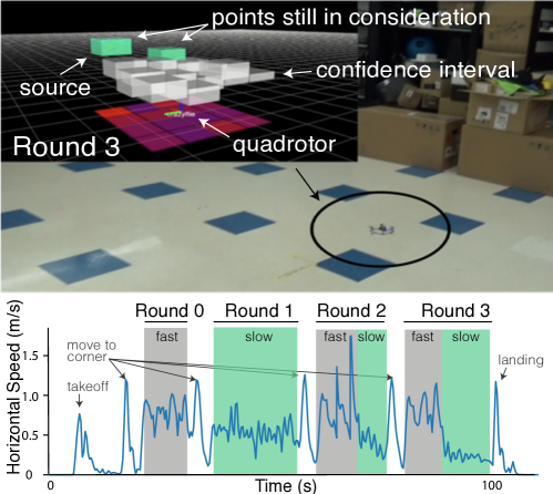
Figure 1: A Crazyflie 2.0 quadrotor in a motion capture room during a hardware demo of $\mathtt{AdaSearch}$ (round 3 of the algorithm). Top: confidence intervals for estimated radioactivity (simulated) within the room. Bottom: horizontal speed over time, indicating slow and fast sections in which $\mathtt{AdaSearch}$ allocates more and fewer sensor measurements, respectively. In later rounds, more time is spent measuring points that are still in consideration (green points).

To overcome these limitations, we introduce $\mathtt{AdaSearch}$, a successive-elimination framework for general source seeking problems with multiple sources, and demonstrate it within the context of RSS. $\mathtt{AdaSearch}$ explicitly maintains confidence intervals over the emissions rate at each point in the environment. Using these confidence intervals, the algorithm identifies a set of candidate points likely to be among the top-$k$ emitters, and eliminates points that are not. Rather than iteratively planning for short, receding time horizons, $\mathtt{AdaSearch}$ repeats a fixed, globally-planned path, adjusting the robot’s speed in real-time to focus measurements on promising regions. This approach offers coverage of the full search space while affording an adaptive measurement allocation in the spirit of information maximization. By maintaining a single fixed, global path, $\mathtt{AdaSearch}$ reduces the online computational overhead, yielding an algorithm easily amenable to real-time implementation.

Specifically, our main contributions are:

• $\mathtt{AdaSearch}$, a general framework for designing efficient sensing trajectories for robotic source seeking problems,

• Theoretical runtime analysis of $\mathtt{AdaSearch}$ as well as of a naive, uniform sampling baseline which follows the same fixed global path but moves at constant speed, and

• Simulation experiments for RSS evaluating $\mathtt{AdaSearch}$ in comparison with a uniform baseline and information maximization.

Our theoretical analysis sharply quantifies $\mathtt{AdaSearch}$’s improvement over its uniform sampling analog. Experiments validate this finding in practice, and also show that $\mathtt{AdaSearch}$ outperforms a custom implementation of information maximization tailored to the RSS problem. Together, these results suggest that the accuracy and efficient runtime of $\mathtt{AdaSearch}$ are robust to heterogeneous background noise, which stands in contrast to existing alternative methods. This robustness is particularly valuable in real-world applications where the exact distribution of background signals in the environment is likely unknown.

The remainder of this paper is organized as follows. Sec. 2 presents a brief survey of related literature. Sec. 3 provides a formal statement of the source seeking problem and introduces our solution, $\mathtt{AdaSearch}$. In Sec. 4, we consider a radioactive source seeking (RSS) case study and develop two appropriate sensing models which allow us to apply $\mathtt{AdaSearch}$ to RSS. Sec. 5 analyzes the theoretical runtime complexity of $\mathtt{AdaSearch}$ and its uniform sampling analog for the RSS problem. In Sec. 6, we present simulation experiments which corroborate these theoretical results. A hardware demonstration provides further evidence of $\mathtt{AdaSearch}$’s potential for real-time application. Sec. 7 suggests a number of extensions and generalizations to $\mathtt{AdaSearch}$, and Sec. 8 concludes with a summary of our results.

2 Related Work

There is a breadth of existing work related to source seeking. Much of this literature, particularly when tailored to robotic applications, leverages some form of information maximization, often using a Gaussian process prior. However, our own work is inspired by approaches from the pure exploration multi-armed bandit literature, even though bandits are not typically used to model physical sensing problems with realistic motion constraints. We survey the most relevant work in both information maximization and multi-armed bandits below.

2.1 Information maximization methods

A popular approach to active sensing and source seeking in robotics, e.g. in active mapping [5] and target localization [6], is to choose trajectories that maximize a measure of information gain [7, 8, 9, 5, 10]. In the specific case of linear Gaussian measurements, Atanasov et al. [11] formulate the informative path planning problem as an optimal control problem that affords an offline solution. Similarly, Lim et al. [12] propose a recursive divide and conquer approach to active information gathering for discrete hypotheses, which is near-optimal in the noiseless case.

Planning for information maximization-based methods typically proceeds with a receding horizon [7, 13, 14, 15, 16]. For example, Ristic et al. [17] formulate information gathering as a partially observable Markov decision process and approximate a solution using a receding horizon. Marchant et al. [13] combine upper confidence bounds (UCBs) at potential source locations with a penalization term for travel distance to define a greedy acquisition function for Bayesian optimization. Their subsequent work [14] reasons at the path level to find longer, more informative trajectories. Noting the limitations of a greedy receding horizon approach, [18] incentivizes exploration by using a look-ahead step in planning. Though similar in spirit to these information seeking approaches, a key benefit of $\mathtt{AdaSearch}$ is that it is not greedy, but rather iterates over a global path.

Information maximization methods typically require a prior distribution on the underlying signals. Many active sensing approaches model this prior as being drawn from a Gaussian process (GP) over an underlying space of possible functions [6, 7, 13], tacitly enforcing the assumption that the sensed signal is smooth [13]. In certain applications, this is well motivated by physical laws, e.g. diffusion [18]. However, GP priors may not reflect the sparse, heterogeneous emissions encountered in radiation detection and similar problem settings.

2.2 Multi-armed bandit methods

$\mathtt{AdaSearch}$ draws heavily on confidence-bound based algorithms from the pure exploration bandit literature [19, 20, 21]. In contrast to these works, our method explicitly incorporates a physical sensor model and allows for efficient measurement allocation despite the physical movement constraints inherent to mobile robotic sensing. Other works have studied spatial constraints in the online, “adversarial” reward setting [22, 23]. Baykal et al. [24] consider spatial constraints in a persistent surveillance problem, in which the objective is to observe as many events of interest as possible despite unknown, time-varying event statistics. Recently, Ma et al. [8] encode a notion of spatial hierarchy in designing informative trajectories, based on a multi-armed bandit formulation. While [8] and $\mathtt{AdaSearch}$ are similarly motivated, hierarchical planning can be inefficient for many sensing models, e.g. for short-range sensors, or signals that decay quickly with distance from the source.

Bandit algorithms are also studied from a Bayesian perspective, where a prior is placed over underlying rewards. For example, Srinivas et al. [25] provide an interpretation of the GP upper confidence bound (GP-UCB) algorithm in terms of information maximization. $\mathtt{AdaSearch}$ does not use such a prior, and is more similar to the lower and upper confidence bound (LUCB) algorithm [26], but opts for successive elimination over the more aggressive LUCB sampling strategy for measurement allocation.

A multi-armed bandit approach to active exploration in Markov decision processes (MDPs) with transition costs is studied in [27], which details trade-offs between policy mixing and learning environment parameters. This work highlights the potential difficulties of applying a multi-armed bandit approach while simultaneously learning robot policies. In contrast, we show that decoupling the use of active learning during the sampling decisions from a fixed global movement path confers efficiency gains under reasonable environmental models.

2.3 Other source seeking methods

Other notable extremum seeking methods include those that emulate gradient ascent in the physical domain [28, 29, 30], take into account specific environment signal characteristics [31], or are specialized for particular vehical dynamics [32]. Modeling emissions as a continuous field, gradient-based approaches estimate and follow the gradient of the measured signal toward local maxima [28, 29, 30]. One of the key drawbacks of gradient-based methods is their susceptibility to finding local, rather than global, extrema. Moreover, the error margin on the noise of gradient estimators for large-gain sensors measuring noisy signals can be prohibitively large [33], as is the case in RSS. Khodayi-mehr et al. [31] handle noisy measurements by combining domain, model, and parameter reduction methods to actively identify sources in steady state advection-diffusion transport system problems such as chemical plume tracing. Their approach combines optimizing an information theoretic quantity based on these approximations with path planning in a feedback loop, specifically incorporating the physics of advection-diffusion problems. In comparison, we consider planning under specific sensor models, and plan motion path and optimal measurement allocation separately.

3 AdaSearch Planning Strategy

3.1 Problem statement

We consider signals (e.g. radiation) which emanate from a finite set of environment points $\mathcal{S}$. Each point $x\in\mathcal{S}$ emits signals $\{\mathbf{X}_{t}(x)\}$ indexed by time $t$ with means $\mu(x)$, independent and identically distributed over time. Our aim is to correctly and exactly discern the set of the $k$ points in the environment that emit the maximal signals:

$$\mathcal{S}^{*}(k)=\operatorname*{arg\,max}_{\begin{subarray}{c}S^{\prime}\subseteq\mathcal{S},|S^{\prime}|=k\end{subarray}}\sum_{x\in S^{\prime}}{\mu(x)}$$ (1)

for a pre-specified integer $1\leq k\leq|\mathcal{S}|$. Throughout, we assume that the set of maximal emitters $\mathcal{S}^{*}(k)$ is unique.

In order to decide which points are maximal emitters, the robot takes sensor measurements along a fixed path ${\mathcal{Z}}=(z_{1},\dots,z_{n})$ in the robot’s configuration space. Measurements are determined by a known sensor model $h(x,z)$ that describes the contribution of environment point $x~{}\in~{}\mathcal{S}$ to a sensor measurement collected from sensing configuration $z\in\mathcal{Z}$. We consider a linear sensing model in which the total observed measurement at time $t$, $\mathbf{Y}_{t}(z)$, taken from sensing configuration $z$, is the weighted sum of the contributions $\{\mathbf{X}_{t}(x)\}$ from all environment points:

$$\mathbf{Y}_{t}(z)=\sum_{x\in\mathcal{S}}h(x,z)\mathbf{X}_{t}(x)$$ (2)

Note that while $h(x,z)$ is known, the $\{\mathbf{X}_{t}\}$ are unknown and must be estimated via the observations $\{\mathbf{Y}_{t}\}$.

The path of sensing configurations, $\mathcal{Z}$, should be as short as possible, while providing sufficient information about the entire environment. This may be expressed as a condition on the minimum aggregate sensitivity $\alpha$ to any given environment point $x$ over the sensing path $\mathcal{Z}$:

$$\sum_{z\in\mathcal{Z}}h(x,z)\geq\alpha>0\quad\forall x\in\mathcal{S}$$ (3)

Moreover, we need to disambiguate between contributions from different environment points $x,x^{\prime}\in\mathcal{S}$. We define the matrix $H\in\mathbb{R}^{|\mathcal{S}|\times|\mathcal{Z}|}$ that encodes the sensitivity of each sensing configuration $z_{j}\in\mathcal{Z}$ to each point $x_{i}\in\mathcal{S}$, so that $H_{ij}:=h(x_{i},z_{j})$. Disambiguation then translates to a rank constraint $\textrm{rank}(H)\geq|\mathcal{S}|$, enforcing invertibility of $HH^{T}$. Sections 4.1 and 4.2 define two specific sensitivity functions that we consider in the context of the RSS problem. In Section 7, we discuss sensitivity functions that may arise in other application domains.

1 Input Candidate points of interest $\mathcal{S}$; sensing path of configurations $\mathcal{Z}$; number of points of interest $k$; minimum measurement duration $\tau_{0}$; procedure for constructing $[\mathrm{LCB}_{i}(x),\mathrm{UCB}_{i}(x)]$ (e.g., as in Sections 4.1 and 4.2); Confidence parameter $\delta_{\mathrm{tot}}$.

2 Initialize $\mathcal{S}^{\mathrm{top}}_{0}=\emptyset,\mathcal{S}_{0}=\mathcal{S}$

3 For rounds $i=0,1,2,\dots$

4 If $\mathcal{S}_{i}=\emptyset$, Return $\mathcal{S}^{\mathrm{top}}_{i}$

5 Choose configuration subset $\mathcal{Z}_{i}\subseteq\mathcal{Z}$ that is informative about environment points $x\in\mathcal{S}_{i}$.

6 Execute a trajectory along path ${\mathcal{Z}}$ that spends time $\tau_{i}=\tau_{0}\cdot 2^{i}$ at each $z\in\mathcal{Z}_{i}$ and time $\tau_{0}$ at each $z\in\mathcal{Z}\setminus\mathcal{Z}_{i}$. Meanwhile, observe signal measurements according to (2).

7 Update $\left[\mathrm{LCB}_{i}(x),\mathrm{UCB}_{i}(x)\right]$ for all $x\in\mathcal{S}$.

8 Update Augment $\mathcal{S}^{\mathrm{top}}_{i}$ according to (4), and prune $\mathcal{S}_{i}$ according to (5).

Algorithm 1 $\mathtt{AdaSearch}$

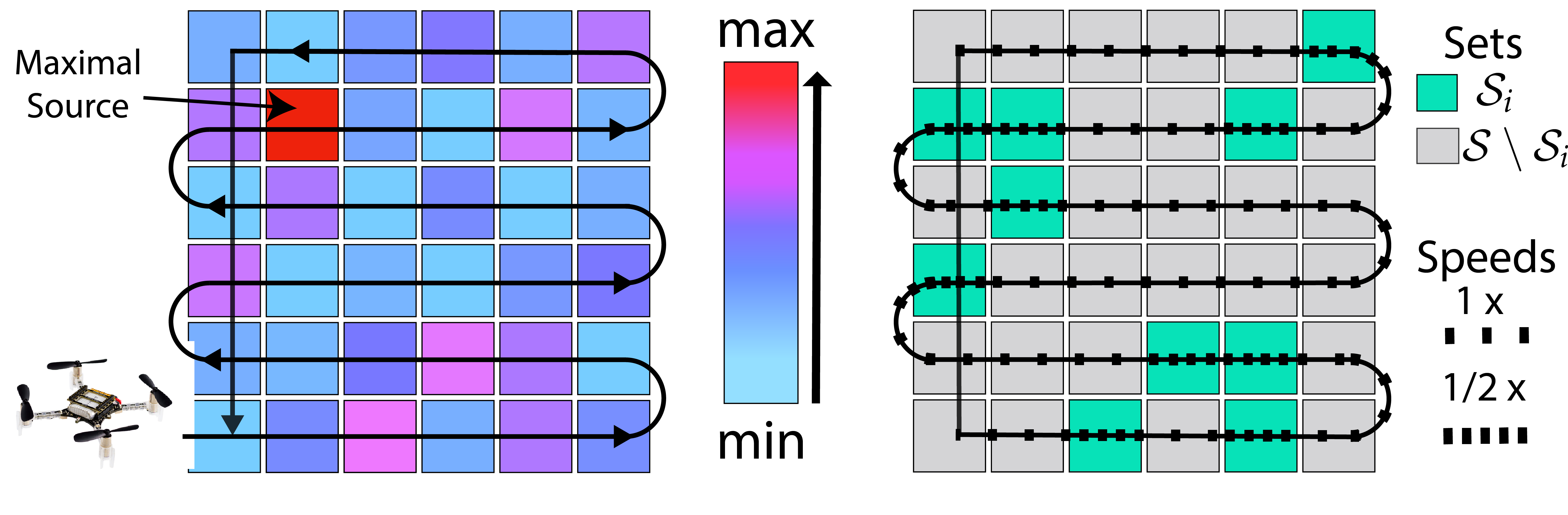
Figure 2: (left) Raster path $\mathcal{Z}$ over an example grid environment of size $6\times 6$. The path ensures that each point is sufficiently measured during each round. (right) Illustrative trajectory for round $i=1$. Dots indicate measurements. $\mathtt{AdaSearch}$ slows to take twice as many measurements over points $x\in\mathcal{S}_{i}$.

3.2 The $\mathtt{AdaSearch}$ algorithm

$\mathtt{AdaSearch}$ (Alg. 1) concentrates measurements in regions of uncertainty until we are confident about which points belong to $S^{*}(k)$. At each round $i$, we maintain a set of environment points $\mathcal{S}^{\mathrm{top}}_{i}$ that we are confident are among the top-$k$, and a set of candidate points $\mathcal{S}_{i}$ about which we are still uncertain. As the robot traverses the environment, new sensor measurements allow us to update the lower and upper confidence bounds

$$\left[\mathrm{LCB}_{i}(x),\mathrm{UCB}_{i}(x)\right]\text{ for each }x\in\mathcal{S}_{i}.$$

and prune the uncertainty set $\mathcal{S}_{i}$. The procedure for constructing these intervals from observations should ensure that for every $x\in\mathcal{S}_{i}$, $\mathrm{LCB}_{i}(x)\leq\mu(x)\leq\mathrm{UCB}_{i}(x)$ with high probability. Sections 4.1 and 4.2 detail the definition of these confidence intervals under different sensing models.

Using the updated confidence intervals, we expand the set $\mathcal{S}^{\mathrm{top}}_{i+1}$ and prune the set $\mathcal{S}_{i+1}$. We add to the top-set $\mathcal{S}^{\mathrm{top}}$ all points $x\in\mathcal{S}_{i}$ whose lower confidence bounds exceed the upper confidence bounds of all but $(k-|\mathcal{S}^{\mathrm{top}}_{i}|)$ points in $\mathcal{S}_{i}$; formally,

$$\mathcal{S}^{\mathrm{top}}_{i+1} \leftarrow\mathcal{S}^{\mathrm{top}}_{i}\cup\{x\in\mathcal{S}_{i}~{}|~{}\mathrm{LCB}_{i}(x)>(k-|\mathcal{S}^{\mathrm{top}}_{i}|+1)\text{-th largest }\mathrm{UCB}_{i}(x^{\prime}),x^{\prime}\in\mathcal{S}_{i}\}.$$ (4)

In Eq. (4), we need not re-evaluate confidence intervals for points $x$ already in $\mathcal{S}^{\mathrm{top}}_{i}$ when producing the set $\mathcal{S}^{\mathrm{top}}_{i+1}$, and can only consider new points. This is explained in the proof of correctness (Lemma 1 and Theorem 2), where we show that with high probability, points $x\notin\mathcal{S}^{*}(k)$ are never incorrectly added to the estimate of the top set $\mathcal{S}^{\mathrm{top}}_{i}$.

Next, the points added to $\mathcal{S}^{\mathrm{top}}_{i+1}$ are removed from $\mathcal{S}_{i+1}$, since we are now certain about them. Additionally, we remove all points in $\mathcal{S}_{i}$ whose upper confidence bound is lower that than the lower confidence bounds of at least $k-|\mathcal{S}^{\mathrm{top}}_{i+1}|$ points in $\mathcal{S}_{i}$. The set $\mathcal{S}_{i+1}$ is defined constructively as:

$$\mathcal{S}_{i+1} \leftarrow\{x\in\mathcal{S}_{i}~{}|~{}x\notin\mathcal{S}^{\mathrm{top}}_{i+1}\text{ and }\mathrm{UCB}_{i}(x)\geq(k-|\mathcal{S}^{\mathrm{top}}_{i+1}|)\text{-th largest }\mathrm{LCB}_{i}(x^{\prime}),x^{\prime}\in\mathcal{S}_{i}\}.$$ (5)

3.3 Trajectory planning for $\mathtt{AdaSearch}$

The update rules (4) and (5) only depend on confidence intervals for points $x\in\mathcal{S}_{i}$. At each round, $\mathtt{AdaSearch}$ chooses a subset of the sensing configurations $\mathcal{Z}_{i}\subseteq\mathcal{Z}$ which are informative to disambiguating the points remaining in $\mathcal{S}_{i}$.

$\mathtt{AdaSearch}$ defines a trajectory by following the fixed path ${\mathcal{Z}}$ over all configurations, slowing down to spend time $2^{i}\tau_{0}$ at informative configurations in $\mathcal{Z}_{i}$, and spending minimal time $\tau_{0}$ at all other configurations in $\mathcal{Z}\setminus\mathcal{Z}_{i}$. Doubling the time spent at each $z\in\mathcal{Z}_{i}$ in each round amortizes the time spent traversing the entire path $\mathcal{Z}$. For omnidirectional sensors, a simple raster pattern (Fig. 2) suffices for ${\mathcal{Z}}$ and choosing $\mathcal{Z}_{i}$ is relatively straightforward (see Sec. 4.3 for further discussion on choosing $\mathcal{Z}$ and $\mathcal{Z}_{i}$). Finally, we remark that one can set the time per configuration $z\in\mathcal{Z}_{i}$ as $\tau_{i}=\tau_{0}c^{i}$ for any constant $c>1$; this yields similar theoretical guarantees, and constants other than $c=2$ may confer slight benefits in practice.

We could also design a trajectory that visits the $z\in\mathcal{Z}_{i}$ and minimizes total travel distance each round, e.g. by approximating a traveling salesman solution. In practice, this would improve upon the runtime of the fixed raster path suggested above. In this work, we use a raster pattern to emphasize the gains due to our main algorithmic components: global coverage and adaptive measurement allocation.

3.4 Correctness

Lemma 1 establishes that the two update rules above guarantee the overall correctness of $\mathtt{AdaSearch}$, whenever the confidence intervals $[\mathrm{LCB}_{j}(x),\mathrm{UCB}_{j}(x)]$ actually contain the correct mean $\mu(x)$:

Lemma 1 (Sufficient Condition for Correctness).

For each round $i\geq 0$, $\mathcal{S}^{\mathrm{top}}_{i}\cap\mathcal{S}_{i}=\emptyset$. Moreover, whenever the confidence intervals satisfy the coverage property:

$$\text{for all rounds }j\leq i~{}\text{ and all }x\in\mathcal{S}_{j},\quad\mu(x)\in[\mathrm{LCB}_{j}(x),\mathrm{UCB}_{j}(x)],$$ (6)

then $\mathcal{S}^{\mathrm{top}}_{i+1}\subseteq\mathcal{S}^{*}(k)\subseteq\{\mathcal{S}^{\mathrm{top}}_{i+1}\cup\mathcal{S}_{i+1}\}$. If (6) holds for all rounds $i$, then $\mathtt{AdaSearch}$ terminates and correctly returns $\mathcal{S}^{*}(k)$.

Proof.

(Sketch) Non-intersection of $\mathcal{S}^{\mathrm{top}}_{i}$ and $\mathcal{S}_{i}$ follows inductively from update rule (5) and the initialization $\mathcal{S}^{\mathrm{top}}_{0}=\emptyset,\mathcal{S}_{0}=\mathcal{S}$.

The overlapping set property $\mathcal{S}^{\mathrm{top}}_{i+1}\subseteq\mathcal{S}^{*}(k)\subseteq\{\mathcal{S}^{\mathrm{top}}_{i+1}\cup\mathcal{S}_{i+1}\}$ follows by induction on the round number $i$. When $i=0$, $\mathcal{S}^{\mathrm{top}}_{0}=\emptyset\subseteq\mathcal{S}^{*}(k)\subseteq\mathcal{S}=\{\mathcal{S}^{\mathrm{top}}_{0}\cup\mathcal{S}_{0}\}$. Now assume that $\mathcal{S}^{\mathrm{top}}_{i}\subseteq\mathcal{S}^{*}(k)\subseteq\{\mathcal{S}^{\mathrm{top}}_{i}\cup\mathcal{S}_{i}\}$ holds for round $i$. Update rule (4) moves a point $x$ from $\mathcal{S}_{i}$ to $\mathcal{S}^{\mathrm{top}}_{i+1}$ only if its LCB is above the $(k+1)$-th largest UCB of all points in $\mathcal{S}_{i}\cup\mathcal{S}^{\mathrm{top}}_{i}$. By (6), $\mathrm{LCB}_{i}(x)\leq\mu(x)\leq\mathrm{UCB}_{i}(x)~{}\forall x\in\mathcal{S}_{i}$, so that $\mu(x)$ must be greater than or equal to the $(k+1)$-st largest means of the points in $\mathcal{S}_{i}\cup\mathcal{S}^{\mathrm{top}}_{i}$. Therefore, this $x$ must belong to $\mathcal{S}^{*}(k)$, establishing that $\mathcal{S}^{\mathrm{top}}_{i+1}\subseteq\mathcal{S}^{*}(k)$. Similarly, by update rule (5), a point $x^{\prime}$ is only removed from $\mathcal{S}^{\mathrm{top}}_{i}\cup\mathcal{S}_{i}$ if its UCB is below the $k$ largest LCBs of points in $\mathcal{S}$, such that $\mu(x^{\prime})$ is less than or equal to at least $k$ other means. Thus, such a point $x^{\prime}$ cannot be in $\mathcal{S}^{*}(k)$. This establishes that $\mathcal{S}^{*}(k)\subseteq\{\mathcal{S}^{\mathrm{top}}_{i+1}\cup\mathcal{S}_{i+1}\}$.

Finally, at termination we have $\mathcal{S}_{i_{\mathrm{fin}}}=\emptyset$, so that $\mathcal{S}^{\mathrm{top}}_{i_{\mathrm{fin}}}\subseteq\mathcal{S}^{*}(k)\subseteq\{\mathcal{S}^{\mathrm{top}}_{i_{\mathrm{fin}}}\cup\mathcal{S}_{i_{\mathrm{fin}}}\}=\mathcal{S}^{\mathrm{top}}_{i_{\mathrm{fin}}}$, so that $\mathcal{S}^{*}(k)=\mathcal{S}^{\mathrm{top}}_{i_{\mathrm{fin}}}$. ∎

Lemma 1 provides a backbone upon which we construct a probabilistic correctness guarantee in Sec. 5. If the event (6) holds over all rounds with some probability $1-\delta_{\mathrm{tot}}$, then $\mathtt{AdaSearch}$ returns the correct set $\mathcal{S}^{*}(k)$ with the same probability $1-\delta_{\mathrm{tot}}$.

4 Radioactive Source-Seeking with Poisson Emissions

While $\mathtt{AdaSearch}$ applies to a range of adaptive sensing problems, for concreteness we now refine our focus to the problem of radioactive source-seeking (RSS) with an omnidirectional sensor. The environment is defined by potential emitter locations which lie on the ground plane, i.e. $x\in\mathcal{S}\subset\mathbb{R}^{2}\times\{0\}$, and sensing configurations encode spatial position, i.e. $z\in\mathcal{Z}\subset\mathbb{R}^{3}$. Environment points emit gamma rays according to a Poisson process, i.e. $\mathbf{X}_{t}(x)\sim\mathrm{Poisson}\left(\mu(x)\right)$. Here, $\mu(x)$ corresponds to rate or intensity of emissions from point $x$.

Thus, the number of gamma rays observed over a time interval of length $\tau$ from configuration $z$ has distribution

$$\mathbf{Y}_{t}(z)\sim\mathrm{Poisson}\Big{(}\tau\cdot\sum_{x\in\mathcal{S}}h(x,z)\mu(x)\Big{)}~{},$$ (7)

where $h(x,z)$ is specified by the sensing model. In the following sections, we introduce two sensing models: a pointwise sensing model amenable to theoretical analysis (Sec. 4.1), and a more physically realistic sensing model for experiments (Sec. 4.2).

In both settings, we develop appropriate confidence intervals for use in the $\mathtt{AdaSearch}$ algorithm. We introduce the specific path used for global trajectory planning in Sec. 4.3. Finally, we conclude with two benchmark algorithms to which we compare $\mathtt{AdaSearch}$ (Sec. 4.4).

4.1 Pointwise sensing model

First, we consider a simplified sensing model, where the set of sensing locations $\mathcal{Z}$ coincides with the set $\mathcal{S}$ of all emitters, i.e. each $z\in\mathcal{Z}$ corresponds to exactly one $x\in\mathcal{S}$ and vice versa. The sensitivity function is defined as ${h(x,z):=\mathbb{I}(x=z)}=[1\textrm{ if }x=z,0\textrm{ if }x\not=z]$.

Now we derive confidence intervals for Poisson counts observed according to this sensing model. Define $\mathbf{N}(x)$ to be the total number of gamma rays observed during the time interval of length $\tau$ spent at $x$. The maximum likelihood estimator (MLE) of the emission rate for point $x$ is $\widehat{\mu}(x)=\frac{\mathbf{N}(x)}{\tau}$. In Appendix B, we introduce the bounding functions $U_{-}(\cdot,\cdot)$ and $U_{+}(\cdot,\cdot)$:

$$U_{+}\left(\mathbf{N},\delta\right) :=2\log(1/\delta)+\mathbf{N}+\sqrt{2\mathbf{N}\log\left(1/\delta\right)}~{}~{}\mathrm{and}$$

$$U_{-}\left(\mathbf{N},\delta\right) :=\max\left\{0,\mathbf{N}-\sqrt{2\mathbf{N}\log(1/\delta)}\right\}$$

Then for any $\lambda\geq 0$, $\mathbf{N}\sim\mathrm{Poisson}(\lambda)$, and $\delta\in(0,1)$,

$$\Pr[U_{-}(\mathbf{N},\delta)\leq\lambda\leq U_{+}(\mathbf{N},\delta)]\geq 1-2\delta.$$

Let $\mathbf{N}_{i}(x)$ denote the number of gammas rays observed from emitter $x$ during round $i$, so that ${\mathbf{N}(x)\sim\mathrm{Poisson}(\tau_{i}\mu(x))}$. For any point $x\in\mathcal{S}_{i}$, the corresponding duration of measurement would be $\tau_{i}$. The bounding functions above provide the desired confidence intervals for signals $\mu(x),\forall x\in\mathcal{S}_{i}$:

$$\mathrm{LCB}_{i}(x):=\frac{1}{\tau_{i}}U_{-}\left(\mathbf{N}_{i}(x),\delta_{i}\right)~{},\quad~{}\mathrm{UCB}_{i}(x):=\tfrac{1}{\tau_{i}}U_{+}\left(\mathbf{N}_{i}(x),\delta_{i}\right)~{},$$ (8)

This bound implies that the inequality ${\tau_{i}\mathrm{LCB}_{i}(x)\leq\tau_{i}\mu(x)\leq\tau_{i}\mathrm{UCB}_{i}(x)}$ holds with probability $1-2\delta_{i}$. Dividing by $\tau_{i}$, we see that $\mathrm{LCB}_{i}(x)$ and $\mathrm{UCB}_{i}(x)$ are valid confidence bounds for $\mu(x)$.

The term $\delta_{i}$ can be thought of as an “effective confidence” for each interval that we construct during round $i$. In order to achieve the correctness in Lemma 1 with overall probability $1-\delta_{\mathrm{tot}}$, we set the effective confidence $\delta_{i}$ at each round to be $\delta_{i}=\delta_{\mathrm{tot}}/{(4|\mathcal{S}|i^{2})}$(see Appendix C.3).

4.2 Physical sensing model

A more physically accurate sensing model for RSS reflects that the gamma ray counts at each location are sensitivity-weighted combinations of emissions from each environment point. Conservation of energy in free space allows us to approximate the sensitivity with an inverse-square law $h(x,z):=c/\|x-z\|_{2}^{2}$, with $c$ a known, sensor-dependent constant. More sophisticated approximations are also possible [17].

Because multiple environment points $x$ contribute to the counts observed from any sensor position $z$, the MLE $\hat{\mu}$ for the emission rates at all $x\in\mathcal{S}$ is difficult to compute efficiently. However, we can approximate it in the limit: $\frac{1}{\sqrt{\tau}}\mathrm{Poisson}(\tau\mu)\overset{d}{\rightarrow}\mathcal{N}\left(\mu,\mu\right)$ as $\tau\rightarrow\infty$. Thus, we may compute $\hat{\mu}$ as the least squares solution:

$$\hat{\mu}=\arg\min_{\vec{\mu}}\|\tilde{H}^{T}\vec{\mu}-\vec{\mathbf{Y}}\|_{2}^{2}~{},$$ (9)

where $\vec{\mu}\in\mathbb{R}^{|\mathcal{S}|}$ is a vector representing the mean emissions from each $x\in\mathcal{S}$, $\vec{\mathbf{Y}}\in\mathbb{R}^{m}$ is a vector representing the observed number of counts at each of $m$ consecutive time intervals, and $\tilde{H}\in\mathbb{R}^{|\mathcal{S}|\times m}$ is a rescaled sensitivity matrix such that $\tilde{H}_{ij}$ gives the measurement-adjusted sensitivity of the $i^{th}$ environment point to the sensor at the $j^{th}$ sensing position. The resulting confidence bounds are given by the standard Gaussian confidence bounds:

$$[\mathrm{LCB}_{i}(x_{k}),\mathrm{UCB}_{i}(x_{k})]:=\hat{\mu}(x_{k})\pm\alpha(\delta_{i})\cdot\Sigma^{1/2}_{kk}~{}\quad\textnormal{where\ }\Sigma:=(\tilde{H}\tilde{H}^{T})^{-1}\enspace$$ (10)

$\alpha(\delta_{i})$ controls the round-wise effective confidence widths in equation (10) as a function of the desired threshold probability of overall error, $\delta_{\mathrm{tot}}$. We use a Kalman filter to solve the least squares problem (9) and compute the confidence intervals (10).

4.3 Design and planning for $\mathtt{AdaSearch}$ : choosing $\mathcal{Z}$ and $\mathcal{Z}_{i}$

Pointwise sensing model. In the pointwise sensing model, $\mathcal{Z}=\mathcal{S}$ and the most informative sensing locations $\mathcal{Z}_{i}$ at round $i$ are precisely $\mathcal{S}_{i}$. We therefore choose the path ${\mathcal{Z}}$ to be a simple space filling curve over a raster grid, which provides coverage of all of $\mathcal{S}$. We adopt a simple dynamical model of the quadrotor in which it can fly at up to a pre-specified top speed, and where acceleration and deceleration times are negligible. This model is suitable for large outdoor environments where travel times are dominated by movement at maximum speed. We denote this maximum speed as $\tau_{0}$. Figure 2 shows an example environment with raster path $\mathcal{Z}$ overlaid (left) and trajectory during round $i=1$ with $\mathcal{Z}_{1}$ shown in teal (right).

Physical sensing model. Because the physical sensitivity follows an inverse-square law, the most informative measurements about $\mu(x)$ are those taken at locations near to $x$. We take measurements at points $z\in\mathbb{R}^{3}$ two meters above points $x\in\mathcal{S}$ on the ground plane. Flying at relatively low height improves the conditioning of the sensitivity matrix $H$. We use the same design and planning strategy as in the pointwise model, following the raster pattern depicted in Fig. 2. More generally, one should chose configurations $z_{i}$ from $\mathcal{Z}_{i}$ so that environment point $x_{i}$ on the ground below each is still in the set of environment points we are unsure about ($\mathcal{S}_{i}$ in Eq. 5).

4.4 Baselines

We compare $\mathtt{AdaSearch}$ to two baselines: a uniform-sampling based algorithm $\mathtt{NaiveSearch}$, and a spatially-greedy information maximization algorithm $\mathtt{InfoMax}$.

NaiveSearch algorithm. As a non-adaptive baseline, we consider a uniform sampling scheme that follows the raster pattern in Fig. 2 at constant speed. This global $\mathtt{NaiveSearch}$ trajectory results in measurements uniformly spread over the grid, and avoids redundant movements between sensing locations. The only difference between $\mathtt{NaiveSearch}$ and $\mathtt{AdaSearch}$ is that $\mathtt{NaiveSearch}$ flies at a constant speed, while $\mathtt{AdaSearch}$ varies its speed. Comparing to $\mathtt{NaiveSearch}$ thus separates the advantages of $\mathtt{AdaSearch}$’s adaptive measurement allocation from the effects of its global trajectory heuristic. Theoretical analysis in Sec. 5 considers a slight variant in which the sampling time is doubled at each round. This doubling has theoretical benefits, but for all experiments we implement the more practical fixed-speed baseline.

InfoMax algorithm. As discussed in Sec. 2, one of the most successful methods for active search in robotics is receding horizon informative path planning, e.g. [14, 15]. We implement $\mathtt{InfoMax}$, a version of this approach based on [14] and specifically adapted for RSS. Each planning invocation solves an information maximization problem over the space of trajectories ${\xi:[t,t+T_{\text{plan}}]\longrightarrow\mathcal{B}}$ mapping from time in the next $T_{\text{plan}}$ seconds to a box $\mathcal{B}\subset{\mathbb{R}}^{3}$.

We measure the information content of a candidate trajectory $\xi$ by accumulating the sensitivity-weighted variance at each grid point $x\in\mathcal{S}$ at $N$ evenly-spaced times along $\xi$, i.e.

$$\xi^{*}_{t}=\arg\max_{\xi}\sum_{i=1}^{N}\sum_{j=1}^{|\mathcal{S}|}\Sigma_{jj}\cdot h\left(x_{j},\xi(t+T_{\text{plan}}i/N)\right)\enspace.$$ (11)

This objective favors taking measurements sensitive to regions with high uncertainty. As a consequence of the Poisson emissions model, these regions will also generally have high expected intensity $\mu$; therefore we expect this algorithm to perform well for the RSS task. We parameterize trajectories $\xi$ as Bezier curves in $\mathbb{R}^{3}$, and use Bayesian optimization (see [34]) to solve (11). Empirically, we found that Bayesian optimization outperformed both naive random search and a finite difference gradient method. We set $T_{\text{plan}}$ to 30 s and used second-order Bezier curves.

Stopping criteria and metrics. All three algorithms use the same stopping criterion, which is satisfied when the $k^{th}$ highest LCB exceeds the $(k+1)^{th}$ highest UCB. For $k=1$ emitter, this corresponds to the first round $i$ in which $\mathrm{LCB}_{i}(x)>\mathrm{UCB}_{i}(x^{\prime}),\forall x^{\prime}\in\mathcal{S}\setminus\{x\}$ for some environment point $x$. For sufficiently small probability of error $\delta_{\mathrm{tot}}$, this ensures that the top-$k$ sources are almost always correctly identified by all algorithms.

5 Theoretical Runtime and Sampling Analysis

Separation of sample-based planning and a repeated global trajectory make $\mathtt{AdaSearch}$ particularly amenable to runtime and sample complexity analysis. We analyze $\mathtt{AdaSearch}$ and $\mathtt{NaiveSearch}$ under the pointwise sensing model from Sec. 4.1. Runtime and sample guarantees are given in Theorem 2, with further analysis for a single source in Corollary 3 to complement experiments. Proofs, along with general results for arbitrary $k$, and complimentary lower bounds, are presented in Appendix B. Simulations (Sec. 6) show that our theoretical results are indeed predictive of the relative performance of $\mathtt{AdaSearch}$ and $\mathtt{NaiveSearch}$.

We analyze $\mathtt{AdaSearch}$ with the trajectory planning strategy outlined in Sec. 4.3. For $\mathtt{NaiveSearch}$, the robot spends time $\tau_{i}$ at each point in each round $i$ until termination, which is determined by the same confidence intervals and termination criterion for $\mathtt{AdaSearch}$.

We will be concerned with the total runtime. Recall that $\tau_{0}$ is the time spent over any point when the robot is moving at maximum speed; $\tau_{i}$ is the time spent sampling candidate points at the slower speed of round $i$.

$$T^{\mathrm{run}} =\begin{cases}\sum_{i=0}^{i_{\mathrm{fin}}}\left(\tau_{i}|\mathcal{S}_{i}|+\tau_{0}|\mathcal{S}\setminus\mathcal{S}_{i}|\right)&(\mathtt{AdaSearch})\\ \sum_{i=0}^{i_{\mathrm{fin}}}\tau_{i}|\mathcal{S}|&(\mathtt{NaiveSearch})\end{cases},$$ (12)

where $i_{\mathrm{fin}}$ is the round at which the algorithm terminates. Bounds are stated in terms of divergences between emission rates $\mu_{2}\geq\mu_{1}>0$:

$$d(\mu_{1},\mu_{2})={(\mu_{2}-\mu_{1})^{2}}/{\mu_{2}}~{}.$$

These divergences approximate the $\mathrm{KL}$-divergence between distributions $\mathrm{Poisson}(\mu_{1})$ and $\mathrm{Poisson}(\mu_{2})$(see Appendix B), and hence the sample complexity of distinguishing between points emitting photons at rates $\mu_{1},\mu_{2}$. Analogous divergences are available for any exponential family, for example Gaussian distributions where the divergences are symmetric.

To achieve the termination criterion (when $\mathcal{S}^{*}(k)$ is determined with confidence $1-\delta_{\mathrm{tot}}$), all points with emission rate below the lowest in $\mathcal{S}^{*}(k)$ must be distinguished from $\mu^{(k)}$, the lowest emission rate of points in $\mathcal{S}^{*}(k)$. Therefore, for points $x\not\in\mathcal{S}^{*}(k)$, we consider divergences $\mathrm{d}(\mu(x),\mu^{(k)})$. Similarly, all points in $\mathcal{S}^{*}(k)$ must be distinguished from the highest background emitter corresponding to the divergences $\mathrm{d}(\mu^{(k+1)},\mu(x))$, describing how close $\mu(x)$ is to the mean rate of the highest background emitter.

Theorem 2.

(Sample and Runtime Guarantees). Define the general adaptive and uniform sample complexity terms $\mathcal{C}_{\mathtt{adapt}}^{(k)}$ and $\mathcal{C}_{\mathtt{unif}}^{(k)}$:

$$\mathcal{C}_{\mathtt{adapt}}^{(k)} :=|S|\tau_{0}+\sum_{x\in\mathcal{S}^{*}(k)}\tfrac{1}{\mathrm{d}(\mu^{(k+1)},\mu(x))}+\sum_{x\in\mathcal{S}\setminus\mathcal{S}^{*}(k)}\tfrac{1}{\mathrm{d}(\mu(x),\mu^{(k)})}$$

$$\mathcal{C}_{\mathtt{unif}}^{(k)} :=|\mathcal{S}|\tau_{0}+|\mathcal{S}|\frac{1}{\mathrm{d}(\mu^{(k+1)},\mu^{(k)})}$$ (13)

$\mathcal{C}_{\mathtt{adapt}}^{(k)}\geq\mathcal{C}_{\mathtt{unif}}^{(k)}$ for any integer number of sources $k\geq 1$ and any distribution of emitters. For any $\delta_{\mathrm{tot}}\in(0,1)$, the following hold each with probability at least $1-\delta_{\mathrm{tot}}$: 
(i) $\mathtt{AdaSearch}$ correctly returns $\mathcal{S}^{*}(k)$, with runtime at most

$$T^{\mathrm{run}}(\mathtt{AdaSearch})\leq~{} \mathcal{C}_{\mathtt{adapt}}^{(k)}\cdot\widetilde{\mathcal{O}}\left(\log({|\mathcal{S}|}/{\delta_{\mathrm{tot}}})\right)$$

$$\quad+\widetilde{\mathcal{O}}\left(|\mathcal{S}|\log_{+}\left({\mathcal{C}_{\mathtt{unif}}^{(k)}}/{|\mathcal{S}|}\right)\right)~{}.$$

(ii) $\mathtt{NaiveSearch}$ correctly returns $\mathcal{S}^{*}(k)$ with runtime bounded by

$$T^{\mathrm{run}}(\mathtt{NaiveSearch})\leq\mathcal{C}_{\mathtt{unif}}^{(k)}\cdot\widetilde{\mathcal{O}}\left(\log(|\mathcal{S}|/\delta_{\mathrm{tot}})\right)~{}.$$

Proof.

(Sketch) The runtimes (12) of each algorithm depend on how quickly we can reduce the set $S_{i}$ in each round. For each point $x$, let $i_{\mathrm{fin}}(x)$ denote the round at which $\mathtt{AdaSearch}$ removes $x$ from $\mathcal{S}_{i}$; at this point we are confident as to whether or not $x$ is in $\mathcal{S}^{*}(k)$, so we do not sample it on successive rounds. At round $i$, we spend time $\tau_{i}=2^{i}$ sampling each point still in $\mathcal{S}_{i}$, so that we spend $\sum_{x\in\mathcal{S}}\sum_{i=0}^{i_{\mathrm{fin}}(x)}\tau_{i}\leq\sum_{x\in\mathcal{S}}2^{1+i_{\mathrm{fin}}(x)}$ time sampling $x$ throughout the run of the algorithm. For $\mathtt{NaiveSearch}$, we sample all points in all rounds, so we spend time $\leq|\mathcal{S}|\max_{x\in\mathcal{S}}2^{1+i_{\mathrm{fin}}(x)}$ sampling.

Now we bound $i_{\mathrm{fin}}(x)$ for each algorithm. These quantities depend on the estimated means $\hat{\mu}_{i}(x)$. Using the concentration bounds that informed the bounding functions in Sec. 4.1, we can form deterministic bounds ${[\overline{\mathrm{LCB}}_{i},\overline{\mathrm{UCB}}_{i}]}$ that depend only on the true means $\mu(x)$. We choose these to encompass the algorithm confidence intervals, so that: $\overline{\mathrm{LCB}}_{i}(x)\leq\mathrm{LCB}_{i}(x)\leq\mu(x)\leq\mathrm{UCB}_{i}(x)\leq\overline{\mathrm{UCB}}_{i}(x)$ with high probability. If each of these inequalities holds with probability $\delta_{\mathrm{tot}}/(4|\mathcal{S}|i^{2})$, then a union bound gives that the probability of failure of any inequality over all rounds is at most $\delta_{\mathrm{tot}}$. By Lemma 1, this ensures correctness with probability at least $1-\delta_{\mathrm{tot}}$.

Because $\overline{\mathrm{LCB}}_{i}(x)$ and $\overline{\mathrm{UCB}}_{i}(x)$ are deterministic given $\mu(x)$ and are contracting to $\mu(x)$ nearly geometrically in $i$, we can bound $i_{\mathrm{fin}}(x)$ by inverting the intervals to find the smallest integer $i$ such that $\overline{\mathrm{LCB}}_{i}(x^{*})>\overline{\mathrm{UCB}}_{i}(x)$ for all $x^{*}\in\mathcal{S}^{*}(k)$ and $x\in\mathcal{S}\setminus\mathcal{S}^{*}(k)$. This requires an inversion lemma from the best arm identification literature (Eq. (110) in [35]). The specific forms of $\overline{\mathrm{LCB}}_{i}$ and $\overline{\mathrm{UCB}}_{i}$ yield the bounds on $i_{\mathrm{fin}}(x)$ in terms of approximate KL divergences, which are added across all environment points to obtain the sample complexity terms for each algorithm in (2).

The form of $\mathcal{C}_{\mathtt{unif}}^{(k)}$ results from noting that the function $(a,b)\mapsto\frac{a}{(a-b)^{2}}$ is decreasing in $a$ and increasing in $b$ for $a>b$, and therefore $\max\left\{\max_{x\in\mathcal{S}^{*}(k)}\frac{1}{\mathrm{d}(\mu^{(k+1)},\mu(x))},\max_{x\in\mathcal{S}\setminus\mathcal{S}^{*}(k)}\frac{1}{\mathrm{d}(\mu(x),\mu^{(k)})}\right\}$ $=1/\mathrm{d}(\mu^{(k+1)},\mu^{(k)}).$ ∎

The $\widetilde{\mathcal{O}}\left(\log(|\mathcal{S}|/\delta_{\mathrm{tot}})\right)$ term in the $\mathtt{AdaSearch}$ runtime bounds accounts for travel times of transitioning between measurement configurations. The second term $|\mathcal{S}|\log(\mathcal{C}_{\mathtt{unif}}/|\mathcal{S}|)$ accounts for the travel time of traversing the uninformative points in the global path ${\mathcal{Z}}$ at a high speed. This term is never larger than $T^{\mathrm{run}}(\mathtt{NaiveSearch})$ and is typically dominated by ${\mathcal{C}_{\mathtt{adapt}}\cdot\widetilde{\mathcal{O}}\left(\log(|\mathcal{S}|/\delta_{\mathrm{tot}})\right)}$. With a uniform strategy, runtime scales with the largest value of $1/d(\mu(x_{1}),\mu(x_{2}))$ over $x_{1}\not\in\mathcal{S}^{*}(k),x_{2}\in\mathcal{S}^{*}(k)$ because that quantity alone determines the number of rounds required. In contrast, $\mathtt{AdaSearch}$ scales with the average of $1/d(\mu(x_{1}),\mu(x_{2}))$ because it dynamically chooses which regions to sample more precisely.

In many scenarios, the number $k$ may estimate the number of hotspots, or there may be more than $k$ sources with similarly high emissions. The extreme case is when emissions $\mu^{(k)}$ and $\mu^{(k+1)}$ are equal, the divergences $\mathrm{d}(\mu^{(k+1)},\mu^{(k)})$ zero. Here the resultant sample complexities $\mathcal{C}_{\mathtt{adapt}}$ and $\mathcal{C}_{\mathtt{unif}}$ are infinite – because no statistical test can distinguish between these two emission $\mu^{(k)}$ and $\mu^{(k+1)}$, the algorithm continues to collect additional samples without terminating. Sec. 5.2 resolves this issue by proposing a simple modification of the stopping condition which returns a set $\widehat{\mathcal{S}}$ of possibly greater than $k$ sources. This modification enjoys similar guarantees to our default termination rule (see Theorem 4).

5.1 Sample complexity for heterogeneous sources

Our sample complexity results qualitatively match standard bounds for active top-$k$ identification with sub-Gaussian rewards in the general multi-armed bandit setting (e.g.  [26]). The following corollary suggests that when the values of $\mathrm{d}(\mu(x),\mu^{*})$ are heterogeneous, $\mathtt{AdaSearch}$ yields significant speedups over $\mathtt{NaiveSearch}$.

Corollary 3.

(Performance under Heterogeneous Background Noise). For a large environment with a single source $x^{*}$ with emission rate $\mu^{*}$ and background signals distributed as $\mu(x)\sim\mathrm{Unif}[0,\overline{\mu}]$ for $x\neq x^{*}$, the ratio of the upper bounds on sample complexities of $\mathtt{AdaSearch}$ to $\mathtt{NaiveSearch}$ scales with the ratio of $\overline{\mu}$ to $\mu^{*}$ as $1-{\overline{\mu}}/{\mu^{*}}.$

Proof.

To control the complexity of $\mathtt{NaiveSearch}$, note

$$\mathcal{C}_{\mathtt{unif}}=\widetilde{\mathcal{O}}(\max_{x\neq x^{*}}{1}/{\mathrm{d}(\mu(x),\mu^{*})})=\widetilde{\mathcal{O}}({\mu^{*}}/{(\mu^{*}-\max_{x\neq x^{*}}\mu(x))^{2}}).$$

It is well known that that the maximum of $N$ uniform random variables on $[0,1]$ is approximately $1-\Theta(\frac{1}{N})$ with probability $1-\Theta(\frac{1}{N})$, implying that $\max_{x\neq x^{*}}\mu(x)\approx(1-\frac{1}{|\mathcal{S}|})\overline{\mu}\approx\overline{\mu}$ with probability at least $1-\Theta({1}/{|\mathcal{S}|})$. Hence, the sample complexity of $\mathtt{NaiveSearch}$ scales as $\widetilde{\mathcal{O}}\left({|\mathcal{S}|\mu_{*}}/{(\overline{\mu}-\mu_{*})^{2}}\right)$. On the other hand, the sample complexity of $\mathtt{AdaSearch}$ grows as

$$\mathcal{C}_{\mathtt{adapt}}=\widetilde{\mathcal{O}}(\sum_{x\neq x^{*}}{1}/{\mathrm{d}(\mu(x),\mu^{*})})=\widetilde{\mathcal{O}}(\sum_{x\neq x^{*}}\mu^{*}(\mu^{*}-\mu(x))^{-2}).$$

When $\mu(x)\sim\mathrm{Unif}[0,\overline{\mu}]$ are random and $|\mathcal{S}|$ is large, the law of large numbers implies that this tends to $\widetilde{\mathcal{O}}\left(\mu^{*}|\mathcal{S}|\cdot\mathbb{E}_{\mu(x)\sim\mathrm{Unif}[0,\overline{\mu}]}{(\mu^{*}-\mu(x))^{-2}}\right)=\widetilde{\mathcal{O}}\left(|\mathcal{S}|(\mu^{*}-\overline{\mu})^{-1}\right)$. Therefore, the ratio of sample bounds of $\mathtt{AdaSearch}$ to $\mathtt{NaiveSearch}$ is $\left(|\mathcal{S}|(\mu^{*}-\overline{\mu})^{-1}\right)/\left({|\mathcal{S}|\mu^{*}}{(\mu^{*}-\overline{\mu})^{-2}}\right)=1-{\overline{\mu}}/{\mu^{*}}$. ∎

5.2 Extension: unknown number of high-emission sources

In many scenarios, there may be considerably more sources of radiation than anticipated. For example, suppose that $\mathtt{AdaSearch}$ is specified with one target source ($k=1$), but in fact there exist two sources $x_{1},x_{2}\in\mathcal{S}$ with $\mu(x_{1})=\mu(x_{2})=\mu^{*}$. Then, $\mathtt{AdaSearch}$ will not terminate with high probability, because it cannot differentiate between these two sources.

To remedy this, we can introduce a slightly more aggressive stopping criterion which will terminate even if multiple sources have similar emissions. The stopping criterion can be stated to terminate if the following holds for an error parameter $\epsilon>0$:

Definition 1 ($\epsilon$-Approximate Termination Rule).

Under the $\epsilon$-approximate termination rule, $\mathtt{AdaSearch}$ either (a) terminates when $\mathcal{S}_{i}=\emptyset$ and returns $\widehat{\mathcal{S}}\leftarrow\mathcal{S}^{\mathrm{top}}_{i}$, or (b) terminates when

$$\min\{\mathrm{LCB}_{i}(x):x\in\mathcal{S}_{i}\}\geq\max\{\mathrm{UCB}_{i}(x):x\in\mathcal{S}_{i}\}-\epsilon.$$ (14)

and returns the union of the sets $\widehat{\mathcal{S}}=\mathcal{S}_{i}\cup\mathcal{S}^{\mathrm{top}}_{i}$.

This criterion will ensure bounded runtime even when there are multiple sources whose mean emissions are close to that of $\mu^{(k)}$. For another possible approach to addressing unknown $k$, we direct the reader to Sec. 7.1. Under the modification of Definition 1, we can modify Theorem 2 as follows. For $\mu_{2}\geq\mu_{1}>0$, introduce

$$\mathrm{d}_{\epsilon}(\mu_{1},\mu_{2}):=\frac{\max\{\mu_{2}-\mu_{1},\epsilon\}^{2}}{\mu_{2}}.$$

Observe that $\mathrm{d}_{\epsilon}(\mu_{1},\mu_{2})\geq\mathrm{d}(\mu_{1},\mu_{2})$, and is always at least $\epsilon^{2}/\mu_{2}$. We define complexity terms analogous to Eq. (2):

$$\mathcal{C}_{\mathtt{adapt}}^{(k)}(\epsilon) :=|S|\tau_{0}+\sum_{x\in\mathcal{S}^{*}(k)}\tfrac{1}{\mathrm{d}_{\epsilon}(\mu^{(k+1)},\mu(x))}$$

$$\qquad+\sum_{x\in\mathcal{S}\setminus\mathcal{S}^{*}(k)}\tfrac{1}{\mathrm{d}_{\epsilon}(\mu(x),\mu^{(k)})}$$

$$\mathcal{C}_{\mathtt{unif}}^{(k)}(\epsilon) :=|\mathcal{S}|\tau_{0}+|\mathcal{S}|\frac{1}{\mathrm{d}_{\epsilon}(\mu^{(k+1)},\mu^{(k)})}$$ (15)

The above describe the adaptive and uniform complexities analogous to those applied in Theorem 2. Essentially, these complexities prevent the runtime from suffering if there are many sources whose emissions are close to that of $\mu^{(k)}$.

Lastly, we introduce a relaxed definition of correctness, which requires that an estimate set $\widehat{\mathcal{S}}$ of the top emitters contains all top emitters $\mathcal{S}^{*}(k)$, and all remaining sources in the set have emissions close to $\mu^{(k)}$.

Definition 2.

A set $\widehat{\mathcal{S}}\subset\mathcal{S}$ is said to be $(k,\epsilon)$-correct if $\widehat{\mathcal{S}}\supseteq\mathcal{S}^{*}(k)$, and for any $x\in\widehat{\mathcal{S}}$, $\mu(x)\geq\mu^{(k)}-\epsilon$.

For the stopping rule in Definition 1 and approximate notion of correctness in Definition 2, Theorem 2 generalizes as follows:

Theorem 4.

(Sample and Runtime Guarantees). For any $\delta_{\mathrm{tot}}\in(0,1)$ and $\epsilon\leq\mu^{(k)}$, the following hold each with probability at least $1-\delta_{\mathrm{tot}}$:
(i) $\mathtt{AdaSearch}$ with the termination rule in Definition 1 returns a $(k,\epsilon)$-correct $\widehat{\mathcal{S}}$ with runtime at most

$$T^{\mathrm{run}}(\mathtt{AdaSearch})\leq~{} \mathcal{C}_{\mathtt{adapt}}^{(k)}(\epsilon)\cdot\widetilde{\mathcal{O}}\left(\log({|\mathcal{S}|}/{\delta_{\mathrm{tot}}})\right)$$

$$\quad+\widetilde{\mathcal{O}}\left(|\mathcal{S}|\log_{+}\left({\mathcal{C}_{\mathtt{unif}}^{(k)}(\epsilon)}/{|\mathcal{S}|}\right)\right)~{}.$$

(ii) $\mathtt{NaiveSearch}$ with the termination rule in Definition 1 returns a $(k,\epsilon)$-correct $\widehat{\mathcal{S}}$ with runtime bounded by

$$T^{\mathrm{run}}(\mathtt{NaiveSearch})\leq\mathcal{C}_{\mathtt{unif}}^{(k)}(\epsilon)\cdot\widetilde{\mathcal{O}}\left(\log(|\mathcal{S}|/\delta_{\mathrm{tot}})\right)~{}.$$

Proof Sketch.

Correctness To see that the modified termination rule returns a $(k,\epsilon)$-correct set, we consider the two possible termination criteria. If the default stopping rule $\mathcal{S}_{i}=\emptyset$, is triggered, then the correctness follows from Theorem 2.

Suppose instead that the stopping rule in Eq. (16) is triggered, so that $\widehat{\mathcal{S}}=\mathcal{S}_{i}\cup\mathcal{S}^{\mathrm{top}}_{i}$. By the original correctness analysis, with high probability, the top emitters are never eliminated from $\mathcal{S}_{i}\cup\mathcal{S}^{\mathrm{top}}_{i}$. Thus, $\widehat{\mathcal{S}}$ contains $\mathcal{S}^{*}(k)$. To prove $(k,\epsilon)$-correctness, let us now show that for any $x\in\widehat{\mathcal{S}}$, $\mu(x)\geq\mu^{(k)}-\epsilon$. With high probability, $\mathcal{S}^{\mathrm{top}}_{i}\subset\mathcal{S}^{*}(k)$ for all rounds $i$, so we will verify this while restricting to $x\in\mathcal{S}_{i}$. We note that on the high probability event that top emitters are never eliminated from $\mathcal{S}_{i}\cup\mathcal{S}^{\mathrm{top}}_{i}$, and if $|\mathcal{S}^{\mathrm{top}}_{i}|<k$, there exists some $x_{0}\in\mathcal{S}^{*}(k)$ such that $x_{0}\in\mathcal{S}_{i}$; for this source, $\mu(x_{0})\geq\mu^{(k)}$. By definition of the stopping rule, we then have

$$\forall x\in\mathcal{S}_{i},\ \ \mathrm{LCB}_{i}(x)\geq\mathrm{UCB}_{i}(x_{0})-\epsilon.$$ (16)

Under the high-probability event that the confidence intervals are correct, this means that

$$\forall x\in\mathcal{S}_{i},\ \ \mu(x)\geq\max\{\mu(x):x\in\mathcal{S}_{i}\}-\epsilon.$$ (17)

Hence, Eq. (17) implies that

$$\forall x\in\mathcal{S}_{i},\mu(x)\geq\mu^{(k)}-\epsilon,$$

as desired.

Sample Complexity Let us now account for the improved sample complexity. In the proof of Theorem 2, we considered an upper bound $i_{\mathrm{fin}}(x)$ on the last round $i$ at which $x\in\mathcal{S}$ remains in $\mathcal{S}_{i}$. The total number of samples where then $2^{i_{\mathrm{fin}}(x)}$, and up to logarithmic factors, this upper bound scaled as $\frac{1}{\mathrm{d}(\mu^{(k+1)},\mu(x))}$ for $x\in\mathcal{S}^{*}(k)$, and with $\frac{1}{\mathrm{d}(\mu(x),\mu^{(k)})}$ for $x\notin\mathcal{S}^{*}(k)$.

For the new stopping rule, we have two cases: if $\mu(x)\notin[\mu^{(k)}-\epsilon/4,\mu^{(k)}+\epsilon/4]$, then the desired sample complexity analysis carries through, as is. This is is because, if $\mu(x)\geq\mu^{(k)}+\epsilon/4$ then $\mathrm{d}_{\epsilon}(\mu^{(k+1)},\mu(x))=\Omega(\mathrm{d}(\mu^{(k+1)},\mu(x))$ (and analogously when $\mu(x)\leq\mu^{(k)}-\epsilon/4$).

Now, consider $i_{0}$ to be sufficiently large that $i_{0}\geq\max\{\inf(x):\mu(x)\notin[\mu^{(k)}-\epsilon/4,\mu^{(k)}+\epsilon/4]\}$. Then, for $i\geq i_{0}$, all that remain are means $\mu(x)\in[\mu^{(k)}-\epsilon/4,\mu^{(k)}+\epsilon/4]$. But once $i$ is sufficiently small that the confidence intervals are at most $\epsilon/8$ in width, all LCB’s and UCB’s will be within, say $\epsilon/4$ of one another, triggering the new stopping condition Eq. (16). Hence, the sample complexity for these means is governed by how many samples are required to shrink these intervals to a width of $\Omega(\epsilon)$, which is roughly bounded by $\frac{\mu^{(k)}+\epsilon/4}{\epsilon^{2}}$. Under the assumption that $\mu^{(k)}\leq\epsilon$, this is at most $\frac{\mu^{(k)}}{\epsilon^{2}}$, which is bounded by $1/\mathrm{d}_{\epsilon}(\mu^{(k)},\mu(x))$ for $x\notin\mathcal{S}^{*}(k)$, and by $1/\mathrm{d}_{\epsilon}(\mu(x),\mu^{(k+1)})$ for $x\in\mathcal{S}^{*}(k)$. ∎

6 Experiments

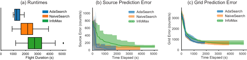
Figure 3: Simulation results of $\mathtt{AdaSearch}$, $\mathtt{NaiveSearch}$ and $\mathtt{InfoMax}$ for 25 randomly instantiated environments with $\overline{\mu}=400$ and $\mu^{*}=800\ \frac{\text{counts}}{\text{s}}$. Lighter shaded areas denote the range of values at each time over $25$ runs of each algorithm; dark lines show the mean. We include final errors for runs that have already finished in max, min, and mean computations. Each algorithm was given the same $25$ randomized grids. (a) Runtimes of $\mathtt{AdaSearch}$, $\mathtt{NaiveSearch}$, and $\mathtt{InfoMax}$ over $25$ random trials. (b) Absolute source error $|\hat{\mu}(x^{*})(t)-\mu(x^{*})|$ over time. (c) Total grid error $\sqrt{\sum_{x\in\mathcal{S}}\|\hat{\mu}(x)(t)-\mu(x)\|_{2}^{2}}$ over time.

We compare the performance of $\mathtt{AdaSearch}$ with the baselines defined in Sec. 4.4 in simulation for the RSS problem with physical sensing model defined in 4.2, and validate $\mathtt{AdaSearch}$ in a hardware demonstration.

6.1 Simulation methodology

We evaluate $\mathtt{AdaSearch}$, $\mathtt{InfoMax}$, and $\mathtt{NaiveSearch}$ in simulation using the Robot Operating System (ROS) framework [36]. Environment points $\mathcal{S}$ lie in a $16\times 16$ planar grid, spread evenly over a total area $64\times 64$ $m^{2}$. Radioactive emissions are detected by a simulated sensor following the physical sensing model given in Sec 4.2 and constrained to fly above a minimum height of $2m$ at all times (see inset of Fig. 1 for simulation setup with $4\times 4$ planar grid environment). For all experiments, we set confidence parameter $\alpha=0.0001$.

For the first set of experiments (Figs. 3, 4), we set $k=1$, so that the set of sources $\mathcal{S}^{*}(k)=\{x^{*}\}$ is a single point in the environment. We set $\mu^{*}=\mu(x^{*})=800$ photons/s. In this setting, we investigate algorithm performance in the face of heterogeneous background signals by varying a maximum environment emission rate parameter $\overline{\mu}\in\{300,400,500,600\}$. For each setting of $\overline{\mu}$, we test all three algorithms on $25$ grids randomly generated with background emission rates drawn uniformly at random from the interval $[0,\overline{\mu}]$.

We also examine the relative performance of all three algorithms as the number of sources increases (Fig. 6). For all experiments with $k>1$, we randomly assign $k$ unique environment points from the grid as the point sources, with emissions rates set to span evenly the range $[800,1000]$ photons/s. The signals of the remaining background emitters are drawn randomly as before, with $\overline{\mu}=400$.

Finally, we examine the relative performance of each algorithm for different environment sizes: square grids with widths $2\times$ and $4\times$ that of the previous experiments (Table 2). To keep the number of sources that must be disambiguated consistent, we instantiate environment points $\mathcal{S}$ in a $16\times 16$ grid, so that the size of each cell changes with the environment scale factor. Here we set $k=1$, $\overline{\mu}=400$, and $\mu^{*}=800$. For the $\mathtt{InfoMax}$ baseline, we adjust the planning horizon to scale with the width of the environment, setting $T_{\text{plan}}=60$ for the doubled grid and $T_{\text{plan}}=120$ for the largest grid.

6.2 Results

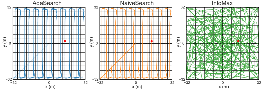
Figure 7: Indicative flight paths for each algorithm. The highest emitting source is denoted by the red dot. $\mathtt{AdaSearch}$ and $\mathtt{NaiveSearch}$ follow a fixed pattern over several rounds, whereas $\mathtt{InfoMax}$ does not.

Figure 3 shows performance across the three algorithms with respect to the following metrics: (a) total runtime (time from takeoff until $x^{*}$ is located with confidence), (b) absolute difference between the predicted and actual emission rate of $x^{*}$, and (c) aggregate difference between predicted and actual emission rates for all environment points $x\in\mathcal{S}$, measured in Euclidean norm. The uniform baseline $\mathtt{NaiveSearch}$ terminates significantly earlier than $\mathtt{InfoMax}$, and $\mathtt{AdaSearch}$ terminates even earlier, on average. Of these $25$ runs, $\mathtt{AdaSearch}$ finished faster than $\mathtt{NaiveSearch}$ in 21 runs, and finished faster than $\mathtt{InfoMax}$ in 24. The flight patterns for the first trial of each algorithm are shown in Fig. 7.

To examine the variation in runtimes due to factors other than the environment instantiation, we also conducted $25$ runs of the same exact environment grid. Due to delays in timing and message passing in simulation (just like there would be in a physical system), measurements of the simulated emissions can still be thought of as random though the environment is fixed. Indeed, the variance in runtimes was comparable to the variance in runtimes in Fig. 3; over the $25$ trials of a fixed grid, the variance in runtimes were $265s$ ($\mathtt{AdaSearch}$), $537s$ ($\mathtt{NaiveSearch}$), and $1028s$ ($\mathtt{InfoMax}$). Of these $25$ runs, $\mathtt{AdaSearch}$ finished faster than $\mathtt{NaiveSearch}$ in 18 runs, and finished faster than $\mathtt{InfoMax}$ in all 25. Fig. 3(b) plots the absolute difference in the estimated emission rate $\hat{\mu}(x^{*})$ and the true emission rate $\mu(x^{*})$ at the one source. $\mathtt{AdaSearch}$ and $\mathtt{NaiveSearch}$ perform comparably over time, and $\mathtt{AdaSearch}$ terminates significantly earlier. Fig. 3(c) plots the Euclidean error between the estimated and the ground truth grids; in this metric the gaps in error between all three algorithms are smaller. $\mathtt{AdaSearch}$ is fast at locating the highest-mean sources without sacrificing performance in total environment mapping.

Fig. 4 shows performance of all three algorithms across different maximum background radiation thresholds $\overline{\mu}$. As $\overline{\mu}$ increases, all algorithms take longer to terminate because the source is harder to distinguish from increasing heterogeneous background signals (left). For high background radiation values (e.g. $\overline{\mu}=600$), the difference in runtimes between all three algorithms is larger; the runtime of $\mathtt{AdaSearch}$ increases gradually under high background signals, whereas $\mathtt{NaiveSearch}$ and $\mathtt{InfoMax}$ are greatly affected. Fig. 5 shows that as $\overline{\mu}$ approaches $\mu^{*}$, the relative speedup of using adaptivity, $T^{\mathrm{run}}(\mathtt{NaiveSearch})/T^{\mathrm{run}}(\mathtt{AdaSearch})$, increases. This is consistent with the theoretical analysis in Sec. 5; the dashed line plots a fit curve with rule $0.7\cdot\mu^{*}/(\mu^{*}-\bar{\mu})$.

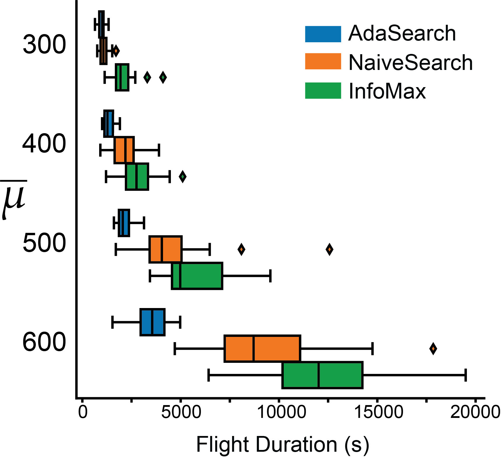
Figure 4: Performance of all three algorithms for grids with maximum background varying, and set as $\overline{\mu}\in\{300,400,500,600\}$, $\mu^{*}=800\ \text{counts}/\text{s}$. For each value of $\overline{\mu}$, each algorithm was given the same 25 randomized grids.

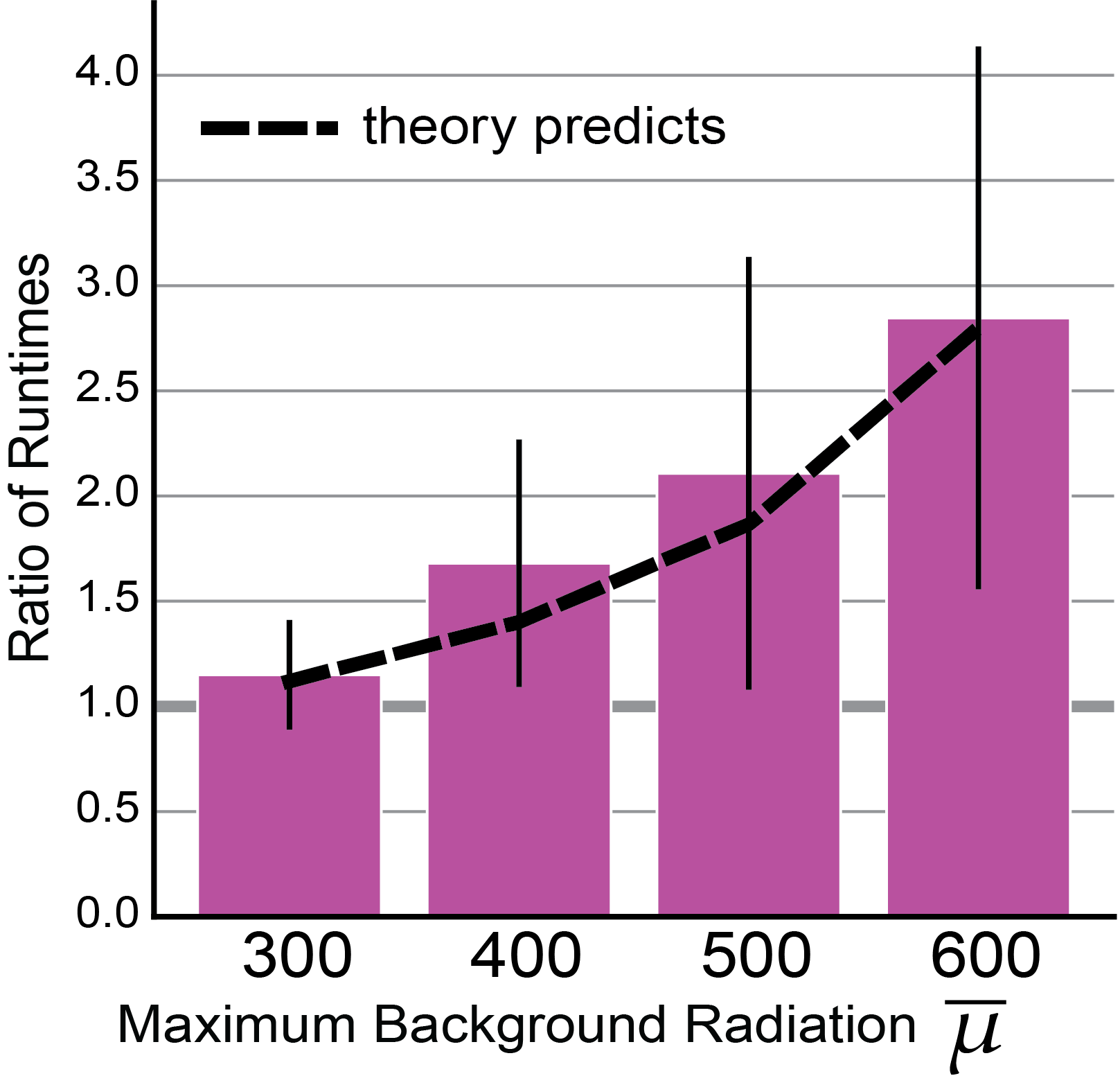
Figure 5: Relative performance of $\mathtt{AdaSearch}$ and $\mathtt{NaiveSearch}$ per random grid, measured as $T^{\mathrm{run}}(\mathtt{NaiveSearch})/T^{\mathrm{run}}(\mathtt{AdaSearch})$; magenta bars indicate mean, and horizontal black lines denote one standard deviation from the mean in either direction. Dashed line shows an approximate fit according to corollary 3. Data is obtained from the same randomized grids as in Fig. 4.

Fig. 6 compares algorithm runtimes across different numbers of sources, $k$. As suggested from Corollary 2, both absolute and relative performance is consistent across $k$ for all three algorithms.

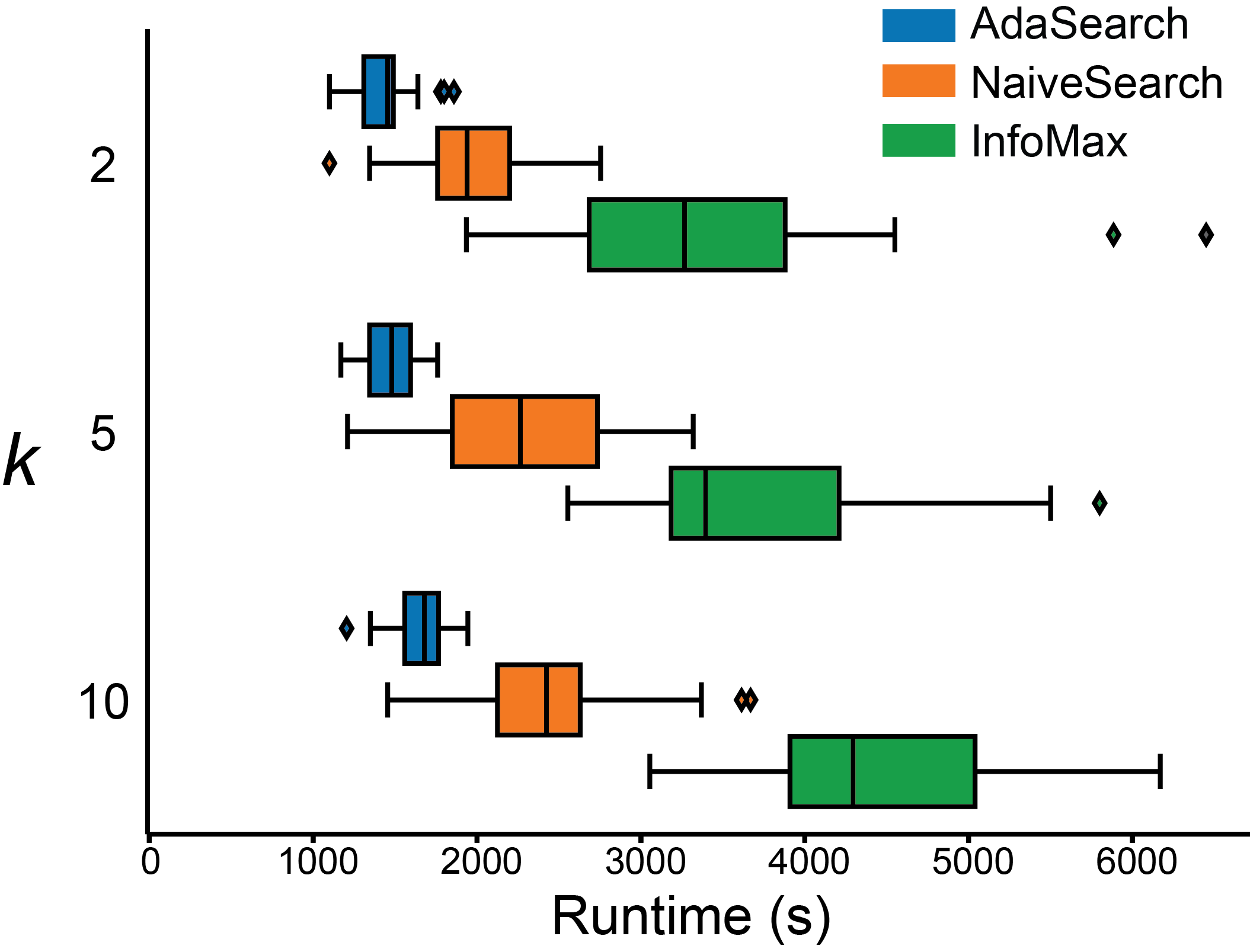
Figure 6: Performance across number of sources, $k$ for $k\in[2,5,10]$. $\mu(x)\in[800,1000]$ for all $x\in\mathcal{S}^{*}(k)$. For each value of $k$, Each algorithm was given the same 25 randomized grids.

The runtimes and number of rounds executed by $\mathtt{AdaSearch}$ and $\mathtt{NaiveSearch}$ for these experiments are summarized in Table 1. In every trial, $\mathtt{AdaSearch}$ takes no more rounds than $\mathtt{NaiveSearch}$ to reach the termination criterion, suggesting that slowing down over informative points saves the algorithm from having to do more entire passes over the environment. Note that each successive round of the $\mathtt{AdaSearch}$ algorithm takes longer than a round of $\mathtt{NaiveSearch}$, since the robot slows down over informative regions, whereas $\mathtt{NaiveSearch}$ does not.

$\mathtt{AdaSearch}$ is inherently a probabilistic algorithm, returning the true sources with probability $1-\delta_{\mathrm{tot}}$, as a function of the number of rounds and the confidence with parameter, $\alpha$. Of the 175 trials run throughout these experiments, $\mathtt{AdaSearch}$ locates the correct source in 174 of them ($99.4\%$). We set $\alpha=0.0001$ in our experiments to facilitate fair comparison of algorithms while maintaining reasonable runtime of the slower methods ($\mathtt{NaiveSearch}$, $\mathtt{InfoMax}$). Given the speed with which $\mathtt{AdaSearch}$ returns a source, in practice it would be feasible to reduce $\alpha$, and hence reduce the probability of a mistake, $\delta_{\mathrm{tot}}$. Due to the good performance of total grid mapping (Fig. 3(c)), even in the low-probability case that an incorrect source is returned, $\mathtt{AdaSearch}$ still provides valuable information about the environment.

Table 1: Round number at time at termination and runtime for $\mathtt{AdaSearch}$ ($\mathtt{Ada}$) and $\mathtt{NaiveSearch}$ ($\mathtt{Naive}$). Averages and standard deviations taken over 25 trials.

		round # at term.: avg (std)		runtime in seconds: avg (std)
k	$\overline{\mu}$	$\mathtt{Ada}$	$\mathtt{Naive}$	$\mathtt{Ada}$	$\mathtt{Naive}$
1	300	3.0 (0.4)	3.8 (0.8)	981 (1778)	1103 (237)
1	400	3.8 (0.6)	7.4 (2.4)	1352 (255)	2208 (694)
1	500	5.0 (0.7)	14.4 (6.8)	2136 (391)	4436 (2145)
1	600	6.6 (0.6)	30.5 (9.5)	3558 (767)	9483 (3004)
2	400	4.0 (0.4)	6.6 (1.2)	1442 (200)	1955 (386)
5	400	3.8 (0.4)	7.8 (2.0)	1465 (167)	2295 (569)
10	400	4.2 (0.5)	8.2 (1.7)	1667 (168)	2502 (532)

The performance of each algorithm for environments at larger scale factors is given in Table 2. Doubling the environment scale factor has two effects on the difficulty of the problem. First, it essentially doubles the flight time to fulfill a "snaking" path across the environment (see Fig. 2). Second, doubling the environment grid width distributes environment points further from each other in space, so that contributions from individual environment points are easier to disambiguate. The results in Table 2 show that for larger grid sizes, both $\mathtt{AdaSearch}$ and $\mathtt{NaiveSearch}$ outperform $\mathtt{InfoMax}$ in terms of runtime. Additionally, the difference in average runtime between $\mathtt{AdaSearch}$ and $\mathtt{NaiveSearch}$ is small for the larger grid sizes ($128\times 128$ and $256\times 256~{}m^{2}$), a consequence of the easier sampling problem (due to dispersed environment points), indicated by a reduced number of rounds needed for the larger grid environments, compared to the $64\times 64~{}m^{2}$ grid. In all runs summarized in Table 2, the algorithms locate the correct source.

Table 2: Runtime for each algorithm with different environment sizes, as well as the round number at termination for $\mathtt{AdaSearch}$ and $\mathtt{NaiveSearch}$. Each grid consists of $16\times 16$ cells with $k=1$ and $\overline{\mu}=400$. Averages and standard deviations taken over 10 trials.

	round # at termination: avg (std)		runtime in seconds: avg (std)
grid size	$\mathtt{AdaSearch}$	$\mathtt{NaiveSearch}$	$\mathtt{AdaSearch}$	$\mathtt{NaiveSearch}$	$\mathtt{InfoMax}$
$64\times 64~{}m^{2}$	3.8 (0.4)	7.6 (2.4)	1345 (229)	2222 (692)	2460 (701)
$128\times 128~{}m^{2}$	2.0 (0.0)	2.4 (0.5)	1356 (170)	1322 (193)	3301 (837)
$256\times 256~{}m^{2}$	1.9 (0.3)	1.9 (0.3)	1916 (548)	2025 (424)	6792 (1949)

6.3 Discussion

While all three methods eventually locate the correct source $x^{*}$ the vast majority of the time, the two algorithms with global planning heuristics, $\mathtt{AdaSearch}$ and $\mathtt{NaiveSearch}$, terminate considerably earlier than $\mathtt{InfoMax}$, which uses a greedy, receding horizon approach (Fig. 3). Moreover, the adaptive algorithm $\mathtt{AdaSearch}$ consistently terminates before its non-adaptive counterpart, $\mathtt{NaiveSearch}$. These trends hold over differing background noise threshold $\overline{\mu}$ and number of sources, $k$ (Figs. 5 and 6).

The $\mathtt{AdaSearch}$ algorithm excels when it can quickly rule out points in early rounds. From (2) we recall that the $\mathtt{AdaSearch}$ sample complexity scales with the average value of $\mu(x)/(\mu^{*}-\mu(x))^{2}$ (rather than the maximum, for $\mathtt{NaiveSearch}$). Hence, $\mathtt{AdaSearch}$ will outperform $\mathtt{NaiveSearch}$ when there are varying levels of background radiation.

As $\overline{\mu}$ approaches $\mu^{*}$ and the gaps $\mu^{*}-\mu(x)$ become more variable, adaptivity confers even greater advantages over uniform sampling. From corollary 3, we expect the ratio of $\mathtt{NaiveSearch}$ runtime to $\mathtt{AdaSearch}$ runtime to scale as ${\mu^{*}}/({\mu^{*}-\overline{\mu}})$, which is corroborated by the fit of the dashed line to the average runtime ratios in Fig. 6. The stability of $\mathtt{AdaSearch}$ in spite of increasing background noise is striking, especially in comparison to the two alternatives presented here; this suggests that in settings where background noise could be misleading to discerning the true signal, a confidence-bound based sampling scheme is likely preferable.

The performance differences between $\mathtt{AdaSearch}$ and $\mathtt{InfoMax}$, and $\mathtt{NaiveSearch}$ hold as the number of sources increases, indicating that $\mathtt{AdaSearch}$ is preferable for a range of different enviroments and source seeking instances.

$\mathtt{InfoMax}$’s strength lies in quickly reducing global uncertainty across the entire emissions landscape. However, $\mathtt{InfoMax}$ takes considerably longer to identify $x^{*}$ (Fig. 3(a)) and, surprisingly, $\mathtt{AdaSearch}$ and $\mathtt{NaiveSearch}$ perform similarly to $\mathtt{InfoMax}$ in mapping the entire emissions landscape on longer time scales (Fig. 3(c)). We attribute this to the effects of greedy, receding horizon planning. Initially, $\mathtt{InfoMax}$ has many locally-promising points to explore and reduces the Euclidean error quickly. Later on, it becomes harder to find informative trajectories that route the quadrotor near the few under-explored regions. The results in Table 2 suggest that this problem remains for larger environments as well. These results suggest that when a path $\mathcal{Z}$ such as the raster path used here is available, it is well worth considering.

High variation in all experiments is expected due to the noisyPoisson emissions signals. While this noise effects the runtime of all algorithms, the range of runtimes for $\mathtt{AdaSearch}$ is consistently tight compared to the other two methods, suggesting that carefully allocated measurements are indeed increasing robustness under heterogeneous background signals.

6.4 Hardware demonstration

The previous results are based on a simulation of two key physical processes: radiation sensing and vehicle dynamics. We also test $\mathtt{AdaSearch}$ on a Crazyflie 2.0 palm-sized quadrotor in a motion capture room with simulated radiation readings. The motion capture data (position and orientation) is acquired at roughly $235$ Hz and processed in real time using precisely the same implementation of $\mathtt{AdaSearch}$ used in our software simulations. Our supplementary video shows a more detailed display of our system. Fig. 1 visualizes the confidence intervals and the absolute source point estimation error, as well as the horizontal speed, during a representative flight over a small $4\times 4$ grid, roughly $3m$ on a side.

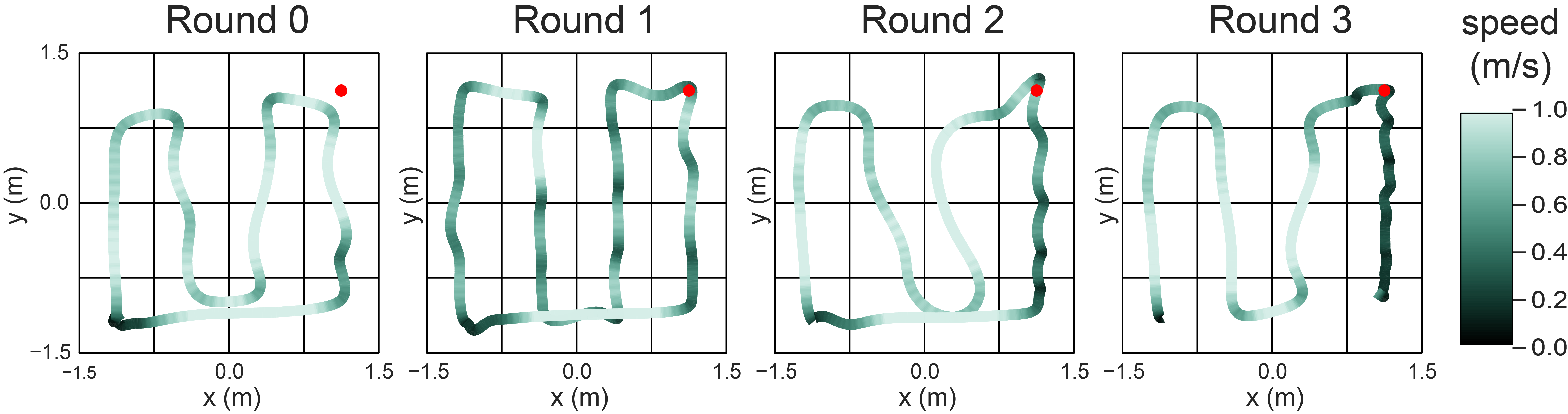
Figure 8: Hardware experiment trajectories for each round of $\mathtt{AdaSearch}$, color coded by speed ($m/s$). The highest emitting source is denoted by the red dot.

Fig. 8 shows the flight paths for each round, color coded by speed (darker is slower). Despite imperfections in following the snake path and velocity changes, the robot’s trajectory successfully represents the algorithm. After two rounds, $\mathtt{AdaSearch}$ identifies the two highest emitting points as the highlighted pixels in the top inset, and the absolute error in estimating $\mu(x^{*})$ is very small. $\mathtt{AdaSearch}$ spends most of its remaining runtime sensing these two points and avoids taking redundant measurements elsewhere. The plot of horizontal speed over time (lower inset of Fig. 1) shows this reallocation of sensor measurements; in the final two rounds, the quadrotor moves quickly at first, then slows down over the two candidate points. This hardware demonstration gives preliminary validation that $\mathtt{AdaSearch}$ is indeed safe and reasonable to use onboard a physical system.

7 Generalizations and Extensions

Before concluding, we briefly discuss several extensions and generalizations of $\mathtt{AdaSearch}$.

7.1 Unknown number of sources

In 5.2, we presented a modified termination criterion which accomodates the possibility of multiple high-emission sources (Defn. 1). This criterion is particularly suitable if there are multiple sources whose emissions are near that of the $k$-th largest source $\mu^{(k)}$. The modified algorithm correctly recovers all top-$k$ sources, as well as possibly returning some additional sources for which emissions $\mu(x)$ are within $\epsilon$ of $\mu^{(k)}$.

In other scenarios, it may be more suitable to return all sources for which emissions $\mu(x)$ are within $\epsilon$ of $\mu^{(k)}$ and no sources whose emission are with a factor of $\epsilon^{\prime}>\epsilon$. With more sophisticated termination criterion and candidate sets $\mathcal{S}^{\mathrm{top}}_{i}$ and $\mathcal{S}_{i}$, $\mathtt{AdaSearch}$ can be modified to accomodate this alternate guarantee. More broadly, the $\mathtt{AdaSearch}$ design principle - combining confidence-interval based elimination with simple raster movement planning - is ammenable to other approximate-search criteria which may arise in given application domains.

We also note that, if one runs $\mathtt{AdaSearch}$ with a small $k$, the algorithm will still collect measurements from other high-emission locations that can re-used if the practicioner wishes to consider a greater number of $k^{\prime}>k$ on a subsequent run.

7.2 Oriented sensor

A natural extension of the radioactive source-seeking example is to consider a sensing model with a sensitivity function which depends upon orientation. The additional challenge lies in identifying informative sensing configuration sets $\mathcal{Z}_{i}$ and a reasonably efficient equivalent fixed global path ${\mathcal{Z}}$. More broadly, the sensing configurations $z\in\mathcal{Z}$ could be taken to represent generalized configurations of the robot and sensor, e.g., they could encode the position and angular orientation of a directional sensor or joint angles of a manipulator arm.

7.3 Pointwise sensing model

We motivated the pointwise sensing model where sensitivity function is $h(x,z)=\mathbb{I}\{x=z\}$ as a model conducive to theoretical analysis. Though it is only a coarse (yet still predictive) approximation of the physical process of radiation sensing, this sensitivity model is a more precise descriptor of other sensing processes. For example, the pointwise model is appropriate for survey design. As a concrete example, suppose an aid group with enough funding to set up $k$ medical clinics sought to identify which $k$ towns had the highest rates of disease. It is reasonable to think that the data collected about town $i$ is mostly informative about only the rate of disease in that town, so that the pointwise sensing model may be quite appropriate.

7.4 Surveying

Although we demonstrate $\mathtt{AdaSearch}$ operating onboard a UAV in the context of RSS, the core algorithm applies more broadly, even to non-robotic embodied sensing problems. Consider the problem of planning $k$ clinic locations. Because surveys are conducted in person, the aid group is resource limited in terms of using human surveyors, both in terms of the time it takes to survey a single person or clinic within a town, and in terms of travel time between towns. A survey planner could use $\mathtt{AdaSearch}$ to guide the decisions of how long to spend in each town counting new cases of the disease before moving on to the next, and to trade-off the travel time of returning to collect more data from a certain town with spending extra time at the town in the first place.

While $\mathtt{AdaSearch}$ provides a good starting point for solving such problems, the high cost of transportation would likely make it worthwhile to further optimize the surveying trajectory at each round, e.g. by (approximately) solving a traveling salesman problem.

8 Conclusion

In summary, we have shown that statistical methods from pure exploration active learning offer a promising, under-explored toolkit for robotic source seeking. Specifically, we have shown that motion constraints need not impede active learning strategies.

Our main contribution, $\mathtt{AdaSearch}$, outperforms a greedy information-maximization baseline in a radioactive source-seeking task. Its success can be understood as a consequence of two structural phenomena: planning horizon and implicit design objective. The information-maximization baseline operates on a receding horizon and seeks to reduce global uncertainty, which means that even if its planned trajectories are individually highly informative, they may lead to suboptimal performance over a long time scale. In contrast, $\mathtt{AdaSearch}$ uses an application-dependent global path that efficiently covers the entire search space and allocates measurements using principled, statistical confidence intervals.

While our results for the problem of RSS are encouraging, it is likely that in may applications, performance could be limited by the range, field of view, or orientation of the sensors. In some cases (e.g. oriented sensors), such limitations could be addressed by the extensions suggested in Sec. 7, and in others, might necessitate new innovations. We are hopeful that the abstraction of sensing models, statistical measurement, and path planning as separate but integrated components of source seeking can guide such future innovations.

$\mathtt{AdaSearch}$ excels in situations with a heterogeneous distribution of the signal of interest; it would be interesting to make a direct comparison with Gaussian process (GP)-based methods in a domain where the smooth GP priors are more appropriate. We also plan to explore active sensing in more complex environments and with dynamic signal sources and more sophisticated sensors (e.g., directional sensors). Furthermore, as $\mathtt{AdaSearch}$ is explicitly designed for general embodied sensing problems, it would be exciting to test it in a wider variety of application domains.

Appendix

Note: this appendix was not peer reviewed as part of the journal publication of this paper. We include it in this report for completeness.

Appendix A Proof of Lemma 1

We verify Lemma 1 given in Section 3. The proof of this lemma holds for any instantiation of Algorithm 1, regardless of the sensing model or the planning strategy.

First, we verify that for each round $i\geq 0$, $\mathcal{S}^{\mathrm{top}}_{i}\cap\mathcal{S}_{i}=\emptyset$. Indeed, at round $i=0$, $\mathcal{S}^{\mathrm{top}}_{i}=\emptyset$, so the bound holds immediately. Suppose by an inductive hypothesis that $\mathcal{S}^{\mathrm{top}}_{i}\cap\mathcal{S}_{i}=\emptyset$ for some $i\geq 0$. Then, for any $x\in\mathcal{S}^{\mathrm{top}}_{i+1}$, we have two cases:

• $x\in\mathcal{S}^{\mathrm{top}}_{i}$. Then, $x\notin\mathcal{S}_{i}$ by the inductive hypothesis, and $\mathcal{S}_{i}\supset\mathcal{S}_{i+1}$ by (5).

• $x$ is added to $\mathcal{S}^{\mathrm{top}}_{i+1}$ via (4). Then $x\notin\mathcal{S}_{i+1}$ by (5).

Next, we verify that if the confidence intervals are correct in all rounds leading up to round $i$, i.e.

$$\text{for all rounds }j\leq i\text{ and all }x\in\mathcal{S}_{j},\quad\mu(x)\in(\mathrm{LCB}_{j}(x),\mathrm{UCB}_{j}(x)),$$ (18)

then $\mathcal{S}^{\mathrm{top}}_{i+1}\subset\mathcal{S}^{*}(k)$, and $\mathcal{S}^{*}(k)\subset\mathcal{S}^{\mathrm{top}}_{i+1}\cup\mathcal{S}_{i+1}$. We again use induction. Initially, we have $\mathcal{S}^{\mathrm{top}}_{0}=\emptyset\subset\mathcal{S}^{*}(k)\subset\mathcal{S}=\mathcal{S}_{0}$. Now, suppose that at round $i$, one has that $\mathcal{S}^{\mathrm{top}}_{i}\subset\mathcal{S}^{*}(k)$, and $\mathcal{S}^{*}(k)\subset\mathcal{S}^{\mathrm{top}}_{i}\cup\mathcal{S}_{i}$.

To show that $\mathcal{S}^{\mathrm{top}}_{i+1}\subset\mathcal{S}^{*}(k)$, it suffices to show that if $x$ is added to $\mathcal{S}^{\mathrm{top}}_{i+1}$, then $x\in\mathcal{S}^{*}(k)$. By the inductive hypothesis there exists $k-|\mathcal{S}^{\mathrm{top}}_{i}|$ elements of $\mathcal{S}^{*}(k)$ in $\mathcal{S}_{i}$. Hence, if $x$ is added to $\mathcal{S}^{\mathrm{top}}_{i+1}$, and if (18) holds, then

$$\mu(x) \geq\mathrm{LCB}_{i}(x)$$

$$>(k-|\mathcal{S}^{\mathrm{top}}_{i}|+1)\text{-th largest value of }\mathrm{UCB}_{i}(x),~{}x\in\mathcal{S}_{i}$$ by (4)

$$\geq(k-|\mathcal{S}^{\mathrm{top}}_{i}|+1)\text{-th largest value of }\mu(x),~{}x\in\mathcal{S}_{i}$$ by (18)

$$\geq(k+1)\text{-th largest value of }\mu(x),x\in\mathcal{S}_{i}\cup\mathcal{S}^{\mathrm{top}}_{i}.$$

Hence, $\mu(x)$ is among the $k$ largest values of $\mu(x)$ for $x\in\mathcal{S}_{i}\cup\mathcal{S}^{\mathrm{top}}_{i}$. Since $\mathcal{S}^{*}(k)\subset\mathcal{S}_{i}\cup\mathcal{S}^{\mathrm{top}}_{i}$, we therefore have that $x\in\mathcal{S}^{*}(k)$.

Similarly, to show $\mathcal{S}^{*}(k)\subset\mathcal{S}_{i+1}\cup\mathcal{S}^{\mathrm{top}}_{i+1}$, it suffices to show that if $x\in\mathcal{S}_{i}\setminus\mathcal{S}_{i+1}$, and $x\notin\mathcal{S}^{\mathrm{top}}_{i+1}$, then $x\notin\mathcal{S}^{*}(k)$. For $x$ such that $x\in\mathcal{S}_{i}\setminus\mathcal{S}_{i+1}$, and $x\notin\mathcal{S}^{\mathrm{top}}_{i+1}$, it follows that

$$\mu(x) \leq\mathrm{UCB}_{i}(x)$$

$$<(k-|\mathcal{S}^{\mathrm{top}}_{i+1}|)\text{-th largest value of }\mathrm{LCB}_{i}(x),~{}x\in\mathcal{S}_{i}$$ by (5)

$$\leq(k-|\mathcal{S}^{\mathrm{top}}_{i+1}|)\text{-th largest value of }\mu(x),~{}x\in\mathcal{S}_{i}$$ by (18)

$$\leq k\text{-th largest value of }\mu(x),x\in\mathcal{S}_{i}\cup\mathcal{S}^{\mathrm{top}}_{i+1}$$

$$\leq k\text{-th largest value of }\mu(x),x\in\mathcal{S},$$

hence $\mu(x)\notin\mathcal{S}^{*}(k)$.

Finally, we verify that if (18) holds at each round, then at the termination round $i_{\mathrm{fin}}$, $\mathcal{S}_{i_{\mathrm{fin}}}=\emptyset$, so that $\mathcal{S}^{\mathrm{top}}_{i_{\mathrm{fin}}}\subset\mathcal{S}^{*}(k)\subset\mathcal{S}^{\mathrm{top}}_{i_{\mathrm{fin}}}\cup\mathcal{S}_{i_{\mathrm{fin}}}=\mathcal{S}^{\mathrm{top}}_{i_{\mathrm{fin}}}$, so that $\mathcal{S}^{*}(k)=\mathcal{S}^{\mathrm{top}}_{i_{\mathrm{fin}}}$.

Appendix B Theoretical Results for Pointwise Sensing

In this appendix, we present formal statements of the measurement complexities provided in Sec. 5 in the main text, and generalize them to the full top-$k$ problem presented in Algorithm 1 of the main text. We also provide specialized bounds for the randomly generated grids considered in our simulations.

Notation: Throughout, we shall use the notation $f\lesssim g$ to denote that there exists a universal constant $C$, independent of problem parameters, for which $f\leq C\cdot g$. We also define $\log_{+}(x):=\max\{1,\log x\}$.

Formal Setup. Throughout, we consider a rectangular grid $\mathcal{S}$ of $|\mathcal{S}|$ points, and let $\mu(x)$ denote the mean emission rate of each point $x\in\mathcal{S}$ in counts/second. We let $\mu^{(k)}$ denote the $k$-th largest mean $\mu(x)$. In the case that $k=1$, we denote $\mu^{*}:=\mu^{(1)}$, and let $x^{*}:=\arg\max_{x\in\mathcal{S}}\mu(x)$ denote the highest-mean point, with emission rate $\mu^{*}:=\mu(x^{*})$. For identifiability, we assume $\mu^{(k)}>\mu^{(k+1)}$.

Measurements. As described in the main text, we assume a point-wise sensing model in which $\mathtt{AdaSearch}$ and $\mathtt{NaiveSearch}$ can measure each point directly. Recall that , at each round $i$, $\mathtt{AdaSearch}$ takes $\tau_{i}:=2^{i}\tau_{0}$ measurements at each point $x\in\mathcal{S}_{i}$, and $\mathtt{NaiveSearch}$ takes $\tau_{i}$ measurements at each $x\in\mathcal{S}$. We let $\mathbf{N}_{i}(x)$ denote the total number of counts collected at position $x$ at round $i$. We further assume that $\mu(x)$ are standardized according to the same time units as $\tau_{0}$, measuring a source of mean $\mu(x)$ for time interval of length $\tau_{i}$ yields counts distributed according to $\mathbf{N}_{i}\sim\mathrm{Poisson}(2^{i}\cdot\mu(x))$. Finally, we shall let $i_{\mathrm{fin}}$ denote the (random) round at which a given algorithm - either $\mathtt{AdaSearch}$ or $\mathtt{NaiveSearch}$ - terminates.

Confidence Intervals At the core of our analysis are rigorous $1-\delta$ upper and lower confidence intervals for Poisson random variables, proved in Sec. E.1:

Proposition 5.

Fix any $\mu\geq 0$ and let $\mathbf{N}\sim\mathrm{Poisson}(\mu)$. Define

$$U_{+}\left(\mathbf{N},\delta\right):=2\log(1/\delta)+\mathbf{N}+\sqrt{2\mathbf{N}\log\left(1/\delta\right)}~{}~{}\mathrm{and}~{}~{}U_{-}\left(\mathbf{N},\delta\right):=\max\left\{0,\mathbf{N}-\sqrt{2\mathbf{N}\log(1/\delta)}\right\}$$ (19)

Then, it holds that $\Pr[\mu>U_{+}(\mathbf{N},\delta)]\leq\delta$ and $\Pr[\mu<U_{-}(\mathbf{N},\delta)]\leq\delta$.

At each round $i$ and $x\in\mathcal{S}_{i}$ ($\mathtt{AdaSearch}$) or $x\in\mathcal{S}$ ($\mathtt{NaiveSearch}$), recall that we use upper and lower confidence intervals

$$\mathrm{LCB}_{i}(x):=\frac{1}{\tau_{i}}U_{-}\left(\mathbf{N}_{i}(x),\delta_{i}\right)~{},\quad~{}\mathrm{UCB}_{i}(x):=\frac{1}{\tau_{i}}U_{+}\left(\mathbf{N}_{i}(x),\delta_{i}\right)~{},\quad\text{where }\delta_{i}:=\delta/{(4|\mathcal{S}|i^{2})}.$$

Trajectory for $\mathtt{AdaSearch}$. $\mathtt{AdaSearch}$ follows a trajectory where, at each round $i$, $\mathtt{AdaSearch}$ spends time $\tau_{i}=2^{i}\cdot\tau_{0}$ measuring each $x\in\mathcal{S}_{i}$, and spends $\tau_{0}$ travel time traveling over each $x\notin\mathcal{S}_{i}$. For the radioactive sensing problem, this is achieved by following the “snaking pattern” depicted in Fig. 2 in the main text, in which the quadrotor speeds up or slows down over each point to match the specified measurement times. We will define the total sample complexity and total run time respectively as

$$T^{\mathrm{sample}}:=\sum_{i=0}^{i_{\mathrm{fin}}}\tau_{i}|\mathcal{S}_{i}|~{}\text{ and }~{}T^{\mathrm{run}}:=T^{\mathrm{sample}}+\sum_{i=0}^{i_{\mathrm{fin}}}\tau_{0}|\mathcal{S}\setminus\mathcal{S}_{i}|$$

The first quantity above captures the total number of measurements taken at points we still wish to measure, and the second captures the total flight time of the algorithm. For simplicity, we will normalize our units of time so that $\tau_{0}=1$.

Trajectory for $\mathtt{NaiveSearch}$. Whereas we implement $\mathtt{NaiveSearch}$ to travel at a constant speed at each point for each round, our analysis will consider a variant where $\mathtt{NaiveSearch}$ halves its speed each round - that is, takes $2^{i}$ measurements at each point for each round; this doubling yields slightly better bounds on sample complexity, and makes $\mathtt{NaiveSearch}$ compare even more favorably compared to $\mathtt{AdaSearch}$ in theory. This results in a total of $2^{i}\tau_{0}|\mathcal{S}|$ measurements per round. For $\mathtt{NaiveSearch}$, the total sample complexity and total run time are equal, and given by

$$T^{\mathrm{run}}=T^{\mathrm{sample}}=|\mathcal{S}|\sum_{i=0}^{i_{\mathrm{fin}}}\tau_{i}.$$

Termination Criterion for $\mathtt{NaiveSearch}$: For an arbitrary number of $k$ emitters, $\mathtt{NaiveSearch}$ terminates at the first round $i$ in which the $k$-th largest lower confidence bound of all points $x\in\mathcal{S}$ is higher than the $(k+1)$-th largest upper confidence bound of all points $x\in\mathcal{S}$.

B.1 Main Results for $k=1$ Emitters

We are now ready to state our main theorems for $k=1$ emitters. Recall the divergence terms

$$\mathrm{d}(\mu_{1},\mu_{2}):=\frac{(\mu_{2}-\mu_{1})^{2}}{\mu_{2}},~{}(\mu_{1}<\mu_{2})$$ (20)

and, in particular,

$$\mathrm{d}(\mu(x),\mu^{*}):=\frac{(\mu^{*}-\mu(x))^{2}}{\mu^{*}},~{}(\mu(x)<\mu^{*})$$

from Section 5. When term $\mathrm{d}(\mu(x),\mu^{*})$ is small, it is difficult to distinguish between $x^{*}$ and $x$. The following lemma shows that $\mathrm{d}(\mu(x),\mu^{*})$ approximates the the $\mathrm{KL}$-divergence between the distribution $\mathrm{Poisson}(\mu(x))$ and $\mathrm{Poisson}(\mu^{*})$:

Lemma 6.

There exists universal constants $c_{1}$ and $c_{2}$ such that, for any $\mu_{2}\geq\mu_{1}>0$,

$$c_{1}\cdot\mathrm{d}(\mu_{1},\mu_{2})\leq\mathrm{KL}(\mathrm{Poisson}(\mu_{1}),\mathrm{Poisson}(\mu_{2}))\leq c_{2}\cdot\mathrm{d}(\mu_{1},\mu_{2}),$$ (21)

where $\mathrm{d}(\mu_{1},\mu_{2})=(\mu_{2}-\mu_{1})^{2}/\mu_{2}$.

Up to log factors, the sample complexities for $\mathtt{AdaSearch}$ and $\mathtt{NaiveSearch}$ in the $k=1$ case are given by $\mathcal{C}_{\mathtt{adapt}}$ and $\mathcal{C}_{\mathtt{unif}}$, respectively, below:

$$\mathcal{C}_{\mathtt{adapt}}:=\sum_{x\in\mathcal{S}\setminus\{x^{*}\}}\left(\tau_{0}+\frac{1}{\mathrm{d}(\mu(x),\mu^{*})}\right) \mathcal{C}_{\mathtt{unif}}=|\mathcal{S}|\left(\tau_{0}+\max_{x\in S}\frac{1}{\mathrm{d}(\mu(x),\mu^{*})}\right)~{},$$ and (22)

Similarly to the definitions in Theorem 2, $\mathcal{C}_{\mathtt{adapt}}$ and $\mathcal{C}_{\mathtt{unif}}$ differ in that $\mathcal{C}_{\mathtt{adapt}}$ considers the sum over all these point-wise complexities, whereas $\mathcal{C}_{\mathtt{unif}}$ replaces this sum with the number of points multiplied by the worst per-point complexity. $\mathcal{C}_{\mathtt{adapt}}$ can be thought of as the complexity of sampling each point $x\neq x^{*}$ the exact number of times to distinguish it from $x^{*}$, whereas $\mathcal{C}_{\mathtt{unif}}$ is the complexity of sampling each point the exact number of times to distinguish the best point from every other point. Note that we always have that $\mathcal{C}_{\mathtt{adapt}}\leq\mathcal{C}_{\mathtt{unif}}$, and in fact $\mathcal{C}_{\mathtt{unif}}$ can be as large as $\mathcal{C}_{\mathtt{adapt}}\cdot|\mathcal{S}|$.

Our first theorem bounds the sample complexity of $\mathtt{AdaSearch}$ for the $k=1$ case presented in Sec. 5 in the main text. We recall that the sample complexity is the total time spent at all $x\in\mathcal{S}_{i}$ until termination:

Theorem 7.

For any $\delta\in(0,1)$, the following holds with probability at least $1-\delta$: $\mathtt{AdaSearch}$ correctly returns $x^{*}$, the total sample complexity is bounded by bounded above by

$$T^{\mathrm{sample}}\lesssim|\mathcal{S}|+\sum_{x\neq x^{*}}\frac{\log_{+}\left(|\mathcal{S}|\log_{+}\left(\tfrac{1}{\mathrm{d}(\mu(x),\mu^{*})}\right)/\delta\right)}{\mathrm{d}(\mu(x),\mu^{*})}~{}=~{}\widetilde{O}\left(|\mathcal{S}|+\sum_{x\neq x^{*}}\frac{\log(|\mathcal{S}|/\delta)}{\mathrm{d}(\mu(x),\mu^{*})}\right),$$

and the runtime is bounded above by

$$T^{\mathrm{run}} \lesssim T^{\mathrm{sample}}+|\mathcal{S}|\log_{+}\left(\log_{+}\tfrac{|\mathcal{S}|}{\delta}\cdot\max_{x\neq x^{*}}\tfrac{1}{\mathrm{d}(\mu(x),\mu^{*})}\right)~{}=~{}\widetilde{\mathcal{O}}\left(\mathcal{C}_{\mathtt{adapt}}\log(|\mathcal{S}|/\delta)+\tau_{0}|\mathcal{S}|\log\left(\tfrac{\mathcal{C}_{\mathtt{unif}}}{|\mathcal{S}|}\right)\right)~{},$$

where $\widetilde{O}(\cdot)$ hides the doubly logarithmic factors in $1/\mathrm{d}(\mu(x),\mu^{*})$.

Theorem 7 is a direct consequence of our more general bound for $k\geq 1$ emitters, given by Theorem 10, which is proved in Sec. C. The next proposition, proved in Sec. D, controls the sample complexity of $\mathtt{NaiveSearch}$:

Theorem 8.

For any $\delta\in(0,1)$, the following holds with probability at least $1-\delta$: $\mathtt{NaiveSearch}$ correctly returns $x^{*}$, and the total runtime is bounded by bounded above by

$$T^{\mathrm{run}}\lesssim|\mathcal{S}|\cdot\left(\max_{x\neq x^{*}}\frac{\log_{+}\left(|\mathcal{S}|\log_{+}\left(\tfrac{1}{\mathrm{d}(\mu(x),\mu^{*})}\right)/\delta\right)}{\mathrm{d}(\mu(x),\mu^{*})}\right) = \widetilde{O}\left(\mathcal{C}_{\mathtt{unif}}\log(|\mathcal{S}|/\delta)\right)~{}.$$

Lastly, we show that our adaptive and uniform sample complexities are near optimal. We prove the following proposition lower bounding the number of samples any adaptive algorithm must take, in Sec. F.1:

Proposition 9.

There exists a universal constant $c$ such that, for any $\delta\in(0,1/4)$, any adaptive sampling which correctly identifies the top emitting point $x^{*}$ with probability at least $1-\delta$ must collect at least

$$c\log(1/\delta)\cdot\mathcal{C}_{\mathtt{adapt}}$$

samples in expectation. Moreover, any uniform sampling allocation which identifies the top emitting point $x^{*}$ with probability at least $1-\delta$ must take at least

$$c\log(1/\delta)\cdot\mathcal{C}_{\mathtt{unif}}$$

samples in expectation.

B.2 Analysis for Top-$k$ Poisson Emitters

In this section, we continue our analysis of $\mathtt{AdaSearch}$, addressing the full problem of identifying the $k$ Poisson emitters with the highest emission rates. Our goal is to identify the unique set

$$\mathcal{S}^{*}(k):=\{x\in\mathcal{S}:\mu(x)\geq\mu^{(k)}\}$$ (23)

To ensure the top-$k$ emitters are unique, we assume that ${\mu^{(k)}>\mu^{(k+1)}}$ (recall that $\mu^{(k)}$ denotes the $k$-th largest value of $\mu(x)$ among all $x\in\mathcal{S}$). The complexity of identifying the top-$k$ emitters can then described in terms of the gaps of the divergence terms

$$\mathrm{d}(\mu^{(k+1)},\mu(x)) =\frac{(\mu(x)-\mu^{(k+1)})^{2}}{\mu(x)},~{}(\mu(x)>\mu^{(k+1)})\quad\text{and }\quad$$

$$\mathrm{d}(\mu(x),\mu^{(k)}) =\frac{(\mu^{(k)}-\mu(x))^{2}}{\mu^{(k)}},\quad(\mu(x)<\mu^{(k)}).$$

For $x\in\mathcal{S}^{*}(k)$, $\mathrm{d}(\mu^{(k+1)},\mu(x))$ describes how close the emission rate $\mu(x)$ is to the “best” alternative in $\mathcal{S}\setminus\mathcal{S}^{*}(k)$. For $x\in\mathcal{S}\setminus\mathcal{S}^{*}(k)$, $\mathrm{d}(\mu(x),\mu^{(k)})$ describes how close $\mu(x)$ is to the mean $\mu^{(k)}$ of the emitter in $\mathcal{S}^{*}(k)$ from which it is hardest to distinguish. The analogues of $\mathcal{C}_{\mathtt{adapt}}$ and $\mathcal{C}_{\mathtt{unif}}$ are then

$$\mathcal{C}_{\mathtt{adapt}}^{(k)} := \sum_{x\in\mathcal{S}^{*}(k)}\frac{1}{\mathrm{d}(\mu^{(k+1)},\mu(x))}+\sum_{x\in\mathcal{S}\setminus\mathcal{S}^{*}(k)}\frac{1}{\mathrm{d}(\mu(x),\mu^{(k)})}\quad\text{and}$$ (24)

$$\mathcal{C}_{\mathtt{unif}}^{(k)} := |\mathcal{S}|\cdot\max\left\{\max_{x\in\mathcal{S}^{*}(k)}\frac{1}{\mathrm{d}(\mu^{(k+1)},\mu(x))},\max_{x\in\mathcal{S}\setminus\mathcal{S}^{*}(k)}\frac{1}{\mathrm{d}(\mu(x),\mu^{(k)})}\right\}=|\mathcal{S}|\mathrm{d}(\mu^{(k+1)}),\mu^{(k)})$$ (25)

where the equality follows by noting that the function $(x,a)\mapsto\frac{x}{(x-a)^{2}}$ is decreasing in $x$ and increasing in $a$ for $x>a$. The following theorem, proved in Sec. C, provides an upper bound on the sample complexity for top-$k$ identification:

Theorem 10.

For any $\delta\in(0,1)$, the following holds with probability at least $1-\delta$: $\mathtt{NaiveSearch}$ correctly returns $\mathcal{S}^{*}(k)$, and the total sample complexity is bounded above by

$$T^{\mathrm{sample}} \lesssim|\mathcal{S}|+\sum_{x\in\mathcal{S}^{*}(k)}\frac{\log_{+}\left(|\mathcal{S}|\log_{+}\left(\frac{1}{\mathrm{d}(\mu^{(k+1)},\mu(x))}\right)/\delta\right)}{\mathrm{d}(\mu^{(k+1)},\mu(x))}+\sum_{x\in\mathcal{S}\setminus\mathcal{S}^{*}(k)}\frac{\mu^{(k)}\log_{+}\left(|\mathcal{S}|\log_{+}\left(\frac{1}{\mathrm{d}(\mu(x),\mu^{(k)})}\right)/\delta\right)}{\mathrm{d}(\mu(x),\mu^{(k)})}$$

$$=\widetilde{\mathcal{O}}\left(\mathcal{C}_{\mathtt{adapt}}^{(k)}\cdot\log(|\mathcal{S}|/\delta)\right),$$

and the total runtime is bounded by

$$T^{\mathrm{run}} \lesssim T^{\mathrm{sample}}+|\mathcal{S}|\log_{+}\left(\frac{\log_{+}\tfrac{|\mathcal{S}|}{\delta}}{\mathrm{d}(\mu^{(k+1)},\mu^{(k)})}\right)~{}=~{}\widetilde{\mathcal{O}}\left(\mathcal{C}_{\mathtt{adapt}}^{(k)}\cdot\log\tfrac{|\mathcal{S}|}{\delta}+|\mathcal{S}|\log_{+}\left(\tfrac{\mathcal{C}_{\mathtt{unif}}^{(k)}}{|\mathcal{S}|}\right)\right)$$

We remark that our sample complexity qualitatively matches standard bounds for active top-$k$ identification with sub-Gaussian rewards in the non-embodied setting (see, e.g. [26]). Our results differ by considering the appropriate modifications for Poisson emissions, as well as accounting for total travel time. Lastly, we have the bound for uniform sampling.

Theorem 11.

For any $\delta\in(0,1)$, the following holds with probability at least $1-\delta$: $\mathtt{NaiveSearch}$ correctly returns $\mathcal{S}^{*}(k)$, and the total runtime is bounded by bounded above by

$$T^{\mathrm{run}}\lesssim\widetilde{\mathcal{O}}\left(\mathcal{C}_{\mathtt{unif}}\right)\cdot\log(|\mathcal{S}|/\delta)~{}.$$

B.3 Predictions for Simulations

We now return to the case $k=1$. We justify the estimates of the complexity terms $\mathcal{C}_{\mathtt{adapt}}$ and $\mathcal{C}_{\mathtt{unif}}$ provided in Sec. 5 of the main text, where $\mu(x)\sim\mathrm{Unif}[0,\overline{\mu}]$ for $x\neq x^{*}$, and $|\mathcal{S}|=256$. To control the complexity of $\mathtt{NaiveSearch}$, we observe that

$$\mathcal{C}_{\mathtt{unif}}=\widetilde{\mathcal{O}}\left(\max_{x\neq x^{*}}\frac{1}{\mathrm{d}(\mu(x),\mu^{*})}\right)=\widetilde{\mathcal{O}}\left(\frac{\mu^{*}}{(\mu^{*}-\max_{x\neq x^{*}}\mu(x))^{2}}\right).$$

It is well known that that the maximum of $N$ uniform random variables on $[0,1]$ is approximately $1-\Theta(\frac{1}{N})$ with probability $1-\Theta(\frac{1}{N})$, which implies that $\max_{x\neq x^{*}}\mu(x)\approx(1-\frac{1}{|\mathcal{S}|})\overline{\mu}\approx\overline{\mu}$ with probability at least $1-\Theta(\frac{1}{|\mathcal{S}|})$. Hence, the sample complexity of $\mathtt{NaiveSearch}$ should scale as

$$\widetilde{\mathcal{O}}\left(\frac{|\mathcal{S}|\mu_{*}}{(\overline{\mu}-\mu_{*})^{2}}\right)$$

On the other hand, the sample complexity of $\mathtt{AdaSearch}$ grows as

$$\widetilde{\mathcal{O}}\left(\sum_{x\neq x^{*}}\frac{1}{\mathrm{d}(\mu(x),\mu^{*})}\right)=\widetilde{\mathcal{O}}\left(\sum_{x\neq x^{*}}\mu^{*}(\mu^{*}-\mu(x))^{-2}\right)$$

When $\mu(x)\sim\mathrm{Unif}[0,\overline{\mu}]$ are random and $|\mathcal{S}|$ is large, the law of large numbers implies that this term tends to $\widetilde{\mathcal{O}}\left(\mu^{*}|\mathcal{S}|\cdot\mathbb{E}_{\mu(x)\sim\mathrm{Unif}[0,\overline{\mu}]}{(\mu^{*}-\mu(x))^{-2}}\right)$. We can then compute

$$\mathbb{E}_{\mu(x)\sim\mathrm{Unif}[0,\overline{\mu}]}{(\mu^{*}-\mu(x))^{-2}} =\frac{1}{\overline{\mu}}\int_{0}^{\overline{\mu}}\frac{1}{(\mu^{*}-t)^{2}}dt~{}=~{}\frac{1}{\overline{\mu}}\int_{\mu^{*}-\overline{\mu}}^{\mu^{*}}\frac{1}{u^{2}}du$$

$$=\frac{1}{\overline{\mu}}\frac{1}{\mu^{*}-\overline{\mu}}-\frac{1}{\mu^{*}}~{}=~{}\frac{1}{\overline{\mu}}\frac{\mu^{*}-(\mu^{*}-\overline{\mu})}{(\mu^{*}-\overline{\mu})\mu^{*}}$$

$$=\frac{1}{\overline{\mu}}\frac{\overline{\mu}}{(\mu^{*}-\overline{\mu})\mu^{*}}=\frac{1}{(\mu^{*}-\overline{\mu})\mu^{*}},$$

Hence, the total complexity scales as

$$\widetilde{\mathcal{O}}\left(\mu^{*}|\mathcal{S}|\cdot\mathbb{E}_{\mu(x)\sim\mathrm{Unif}[0,\overline{\mu}]}{(\mu^{*}-\mu(x))^{-2}}\right)=\widetilde{\mathcal{O}}\left(|\mathcal{S}|(\mu^{*}-\overline{\mu})^{-1}\right)$$

Therefore, the ratio of the runtimes of $\mathtt{AdaSearch}$ to $\mathtt{NaiveSearch}$ are

$$\frac{\mu^{*}-\overline{\mu}}{\mu^{*}}=1-\frac{\overline{\mu}}{\mu^{*}}.$$

Appendix C Analyzing $\mathtt{AdaSearch}$: Proof of Theorem 10

C.1 Analysis Roadmap

To simplify the analysis, we assume that at round $i$, we take a fresh $\tau_{i}=2^{i}$ samples (recall we have normalized $\tau_{0}=1$) from each remaining $x\in\mathcal{S}_{i}$. For $x\in\mathcal{S}_{i}$, $\mathbf{N}_{i}(x)$ denotes the number of counts observed from point $x$ over the interval of length $\tau_{i}$, and $\widehat{\mu}_{i}(x)$ denotes the empirical average emissions; that is, $\widehat{\mu}_{i}(x)=\mathbf{N}_{i}(x)/\tau_{i}$. With this notation, our confidence intervals take the following form:

$$\mathrm{LCB}_{i}(x):=\frac{1}{2^{i}}U_{-}\left(\mathbf{N}_{i}(x),\frac{\delta}{4|\mathcal{S}|i^{2}}\right)~{}\text{and}~{}\mathrm{UCB}_{i}(x):=\frac{1}{2^{i}}U_{+}\left(\mathbf{N}_{i}(x),\frac{\delta}{4|\mathcal{S}|i^{2}}\right)$$ (26)

We first argue that there exists a good event, $\mathcal{E}_{\mathrm{good}}(\delta)$, occuring with probability at least $1-\delta$, on which the true mean $\mu(x)$ of each pixel $x$ lies between $\mathrm{LCB}_{i}(x)$ and $\mathrm{UCB}_{i}(x)$ for all $i$. Moreover, $\mathrm{LCB}_{i}(x)$ and $\mathrm{UCB}_{i}(x)$ are contained within the interval defined by $[\overline{\mathrm{UCB}}_{i}(x),\overline{\mathrm{LCB}}_{i}(x)]$, which depends explicitly upon $\mu(x)$, but not on $\widehat{\mu}_{i}(x)$. To derive $\overline{\mathrm{UCB}}_{i}(x)$ and $\overline{\mathrm{LCB}}_{i}(x)$, we begin by deriving high probability upper and lower bounds $\overline{U}_{+}(\mu,\delta)$ and $\overline{U}_{-}(\mu,\delta)$ for the functions $U_{+}(\mathbf{N},\delta)$ and $U_{-}(\mathbf{N},\delta)$ that hold for Poisson random variables. Formally, we have the following

Proposition 12.

Let $\mu\geq 0$ and let and $\mathbf{N}\sim\mathrm{Poisson}(\mu)$. Define

$$\overline{U}_{+}(\mu,\delta) := \mu+\frac{14}{3}\log\left(1/\delta\right)+2\sqrt{2\mu\log\left(1/\delta\right)}~{}~{}\mathrm{and}$$

$$\overline{U}_{-}\left(\mu,\delta\right) := \max\left\{0,\mu-2\sqrt{2\mu\log\left(1/\delta\right)}\right\}~{}.$$

Then, it holds that

$$\Pr\left[\overline{U}_{-}(\mu,\delta)\leq U_{-}(\mathbf{N},\delta)\leq\mu\leq U_{+}(\mathbf{N},\delta)\leq\overline{U}_{+}(\mu,\delta)\right]\geq 1-2\delta~{}.$$ (27)

As a consequence of Proposition 12, we can show that $\overline{\mathrm{LCB}}_{i}(x)$ and $\overline{\mathrm{UCB}}_{i}(x)$ are probabilistic lower and upper bounds on $\mathrm{LCB}_{i}(x)$ and $\mathrm{UCB}_{i}(x)$:

Lemma 13.

Introduce the confidence intervals

$$\overline{\mathrm{LCB}}_{i}(x):=\frac{1}{\tau_{i}}\overline{U}_{-}\left(\tau_{i}\mu(x),\frac{\delta}{4|\mathcal{S}|i^{2}}\right)~{}\text{and}~{}\overline{\mathrm{UCB}}_{i}(x):=\frac{|S|}{\tau_{i}}\overline{U}_{+}\left(\tau_{i}\mu(x),\frac{\delta}{4|\mathcal{S}|i^{2}}\right)~{}.$$

Then, there exists an event $\mathcal{E}_{\mathrm{good}}$ for which $\Pr[\mathcal{E}_{\mathrm{good}}]\geq 1-\delta$, and

$$\forall i\geq 1,x\in\mathcal{S}_{i}:\overline{\mathrm{LCB}}_{i}(x)\leq\mathrm{LCB}_{i}(x)\leq\mu(x)\leq\mathrm{UCB}_{i}(x)\leq\overline{\mathrm{UCB}}_{i}(x)~{}.$$ (28)

Lemma 13 is a simple consequence of Propositions 5 and 12, and a union bound; it is proved formally in Sec C.3. Note that on $\mathcal{E}_{\mathrm{good}}$, one has that $\mu(x)\in[\mathrm{LCB}_{i}(x),\mathrm{UCB}_{i}(x)]$ for all rounds $i$ and all $x\in\mathcal{S}_{i}$; hence, by Lemma 1,

Lemma 14.

If $\mathcal{E}_{\mathrm{good}}$ holds, then for all rounds $i$, $\mathcal{S}^{\mathrm{top}}_{i}\subset\mathcal{S}^{*}(k)\subset\mathcal{S}^{\mathrm{top}}_{i}\cup\mathcal{S}_{i}$; in particular, if $\mathtt{AdaSearch}$ terminates at round $i_{\mathrm{fin}}$, then it correctly returns $\mathcal{S}^{*}(k)$.

Finally, the next lemma, proven in C.4, gives a deterministic condition under which a point $x\in\mathcal{S}$ can be removed from $\mathcal{S}_{i}$, in terms of the deterministic confidence bounds $\overline{\mathrm{LCB}}_{i}(x)$ and $\overline{\mathrm{UCB}}_{i}(x)$.

Lemma 15.

Suppose $\mathcal{E}_{\mathrm{good}}$ holds. Let $x^{(k)}$ and $x^{(k+1)}$ denote arbitrary points in $\mathcal{S}$ with $\mu(x^{(k)})=\mu^{(k)}$ and $\mu(x^{(k+1)})=\mu^{(k+1)}$. Define the function

$$i_{\mathrm{fin}}(x):=\begin{cases}\inf\{i:\overline{\mathrm{LCB}}_{i}(x)>\overline{\mathrm{UCB}}_{i}(x^{(k+1)})\}&x\in\mathcal{S}^{*}(k)\\ \inf\{i:\overline{\mathrm{UCB}}_{i}(x)<\overline{\mathrm{LCB}}_{i}(x^{(k)})\}&x\in\mathcal{S}\setminus\mathcal{S}^{*}(k)\end{cases}$$

Then, on $\mathcal{E}_{\mathrm{good}}$, $x\notin\mathcal{S}_{i}$ for all $i>i_{\mathrm{fin}}(x)$.

In view of Lemma 15, we can bound

$$T^{\mathrm{sample}} :=\sum_{i=0}^{i_{\mathrm{fin}}}\tau_{i}|\mathcal{S}_{i}|~{}=~{}\sum_{x\in\mathcal{S}}\sum_{i\geq 0}\tau_{i}\mathbb{I}(x\in\mathcal{S}_{i})~{}\leq~{}\sum_{x\in\mathcal{S}}\sum_{i=0}^{i_{\mathrm{fin}}(x)}\tau_{i}\quad(\text{by Lemma}~{}\ref{lem:stop_sampling})$$

$$\leq\sum_{x\in\mathcal{S}}2^{i_{\mathrm{fin}}(x)+1}\quad(\text{since }\tau_{i}=2^{i})$$ (29)

and further, bound

$$T^{\mathrm{run}} :=T^{\mathrm{sample}}+\sum_{i=0}^{i_{\mathrm{fin}}}\tau_{0}|\mathcal{S}\setminus\mathcal{S}_{i}|~{}\leq~{}T^{\mathrm{sample}}+|\mathcal{S}|i_{\mathrm{fin}}\quad(\text{recall}~{}\tau_{0}=1)$$

$$\leq T^{\mathrm{sample}}+|\mathcal{S}|\max_{x\in\mathcal{S}}i_{\mathrm{fin}}(x).$$ (30)

where again the last line uses Lemma 15. Lastly, we prove an upper bound on $i_{\mathrm{fin}}(x)$ for all $x\in\mathcal{S}$, which follows from algebraic manipulations detailed in Sec. C.2:

Proposition 16.

There exists a universal constant $C>1$ such that, for $x\in\mathcal{S}^{*}(k)$,

$$2^{i_{\mathrm{fin}}(x)}\leq C\cdot\left\{1+\frac{\log_{+}\left(|\mathcal{S}|\log_{+}\left(\frac{1}{\mathrm{d}(\mu^{(k+1)},\mu(x))}\right)/\delta\right)}{\mathrm{d}(\mu^{(k+1)},\mu(x))}\right\}$$

whereas for $x\in\mathcal{S}\setminus\mathcal{S}^{*}(k)$,

$$2^{i_{\mathrm{fin}}(x)}\leq C\cdot\left\{1+\frac{\log_{+}\left(|\mathcal{S}|\log_{+}\left(\frac{1}{\mathrm{d}(\mu^{(k+1)},\mu(x))}\right)/\delta\right)}{\mathrm{d}(\mu^{(k+1)},\mu(x))}\right\}$$

Theorem 10 now follows by plugging in Propostion 16 into Equations (29) and (30).

C.2 Proof of Proposition 16

Let $n=2^{i}$, let $\delta_{0}=\delta/(4|\mathcal{S}|\log_{2}e)$, and let $\Delta=\mu(x_{1})-\mu(x_{2})$. Then $\overline{\mathrm{UCB}}_{i}(x_{2})<\overline{\mathrm{LCB}}_{i}(x_{1})$ is equivalent to

$$\mu(x_{2})+\frac{14}{3n}\log\left(\delta_{0}^{-1}\log n\right)+2\sqrt{2\mu(x_{2})\log\left(\delta_{0}^{-1}\log n\right)/n}<\mu(x_{1})-2\sqrt{2\mu(x_{1})\log\left(\delta_{0}^{-1}\log n\right)/n}$$

$$\text{implied by}~{}~{}\frac{14}{3n}\log\left(\delta_{0}^{-1}\log n\right)+4\sqrt{2\mu(x_{1})\log\left(\delta_{0}^{-1}\log n\right)/n}<\Delta~{},$$

where the second line uses $\mu(x_{2})\leq\mu(x_{1})$. For the second line to hold, it is enough that

$$\frac{1}{n}\log\left(\delta_{0}^{-1}\log n\right)<\frac{3\Delta}{28}\text{ and }\log\left(\delta_{0}^{-1}\log n\right)/n<\left(\frac{\Delta}{8\sqrt{2}}\right)^{2}$$ (31)

We now invoke an inversion lemma from the best arm identification literature (see, e.g. Equation (110) in [35]).

Lemma 17.

For any $\delta,u>0$, let $\mathcal{T}(u,\delta):=1+\log_{+}(\delta^{-1}\log_{+}(u))/u$. There exists a universal constant $C_{0}$ such that, for all $n\geq C_{0}\mathcal{T}(u,\delta)$, we have $\log(\delta^{-1}\log n)/n<u$.

Hence, Lemma 17 and (31) imply that it is sufficent that

$$n\geq C_{0}\mathcal{T}\left(\min\left\{\frac{3\Delta}{28},\frac{1}{\mu(x_{1})}\left(\frac{\Delta}{8\sqrt{2}}\right)^{2}\right\},\delta_{0}\right)~{},$$

from which it follows that

$$\inf\left\{2^{i}:\overline{\mathrm{UCB}}_{i}(x_{2})<\overline{\mathrm{LCB}}_{i}(x_{1})\right\}\leq 2C_{0}\left\{\mathcal{T}\left(\min\left\{\frac{3\Delta}{28},\frac{1}{\mu(x_{1})}\left(\frac{\Delta}{8\sqrt{2}}\right)^{2}\right\},\delta_{0}\right)~{}\right\}$$

Absorbing constants and plugging in $\delta_{0}=\delta/(4|\mathcal{S}|\log_{2}e)$, algebraic manipulation finally implies that there exists a universal constant $C$ such that, for any $x_{1},x_{2}$ with $\mu(x_{1})<\mu(x_{2})$,

$$\inf\left\{2^{i}:\overline{\mathrm{UCB}}_{i}(x_{1})<\overline{\mathrm{LCB}}_{i}(x_{2})\right\} \leq C\left\{1+\mathcal{T}\left(\min\left\{\Delta,\frac{\Delta^{2}}{\mu(x_{1})}\right\},\delta/M\right)\right\}$$

$$= C\left\{1+\mathcal{T}\left(\frac{\Delta^{2}}{\mu(x_{1})},\delta/|\mathcal{S}|\right)\right\}~{}$$

$$= C\left\{1+\mathcal{T}\left(\mathrm{d}(\mu(x_{2}),\mu(x_{1})),\delta/|\mathcal{S}|\right)\right\}~{}.$$

To conclude, we select $x_{1}=x^{(k+1)}$ and $x_{2}=x$ when $x\in\mathcal{S}^{*}(k)$, and $x_{1}=x$ and $x_{2}=x^{(k)}$ for $x\in\mathcal{S}\setminus\mathcal{S}^{*}(k)$.

C.3 Proof of Lemma 13

$$\Pr\left[\exists x\in\mathcal{S}_{0},i\geq 1:\left\{\overline{\mathrm{LCB}}_{i}(x)\leq\mathrm{LCB}_{i}(x)\leq\mu(x)\leq\mathrm{UCB}_{i}(x)\leq\overline{\mathrm{UCB}}_{i}(x)\right\}\text{ fails}\right]$$

$$\overset{\text{union bound}}{\leq} \sum_{x\in\mathcal{S}_{0},i\geq 1}\Pr\left[\left\{\overline{\mathrm{LCB}}_{i}(x)\leq\mathrm{LCB}_{i}(x)\leq\mu(x)\leq\mathrm{UCB}_{i}(x)\leq\overline{\mathrm{UCB}}_{i}(x)\right\}\text{ fails}\right]$$

$$\overset{\text{Prop.}~{}\ref{prop:poisson_conc1}\&\ref{prop:poisson_conc2}}{\leq} \sum_{x\in\mathcal{S}_{0},i\geq 1}\frac{\delta}{2|\mathcal{S}|i^{2}}~{}=~{}|\mathcal{S}|\sum_{i\geq 1}\frac{\delta}{2|\mathcal{S}|i^{2}}~{}=~{}\frac{\delta}{2}\sum_{i}i^{-2}~{}\leq~{}\delta~{}.$$

C.4 Proof of Lemma 15

Assume $\mathcal{E}_{\mathrm{good}}$ holds, and let $x\in\mathcal{S}$, and set $i=i_{\mathrm{fin}}(x)$. Then

• If $x\in\mathcal{S}^{*}(k)$, then $\overline{\mathrm{LCB}}_{i}(x)>\overline{\mathrm{UCB}}_{i}(x^{(k+1)})$. In this case, we shall show that $x$ will be added to $\mathcal{S}^{\mathrm{top}}_{i}$ via (4).

• If $x\in\mathcal{S}\setminus\mathcal{S}^{*}(k)$, then $\overline{\mathrm{UCB}}_{i}(x)<\overline{\mathrm{LCB}}_{i}(x^{(k)})$. In this case, we shall show that $x$ will be removed from $\mathcal{S}_{i}$ via (5).

Case 1: $\overline{\mathrm{LCB}}_{i}(x)>\overline{\mathrm{UCB}}_{i}(x^{(k+1)})$ By (4), $x$ is added to $\mathcal{S}^{\mathrm{top}}_{i+1}$ if $\mathrm{LCB}_{i}(x)$ is larger than all but $k-|\mathcal{S}^{\mathrm{top}}_{i}|$ values of $\mathrm{UCB}_{i}(x^{\prime})$, $x^{\prime}\in\mathcal{S}_{i}$. Since $\mathrm{LCB}_{i}(x)\geq\overline{\mathrm{LCB}}_{i}(x)$ and $\mathrm{UCB}_{i}(x^{\prime})\leq\overline{\mathrm{UCB}}_{i}(x^{\prime})$ on $\mathcal{E}_{\mathrm{good}}$, it is enough that

$$\overline{\mathrm{LCB}}_{i}(x)>(k-|\mathcal{S}^{\mathrm{top}}_{i}|+1)\text{-st largest value of }\overline{\mathrm{UCB}}_{i}(x^{\prime}),~{}x^{\prime}\in\mathcal{S}_{i}.$$

We now observe that $\overline{\mathrm{UCB}}_{i}(x^{\prime})$ is monotonic in $\mu(x^{\prime})$. Hence, it is enough that

$$\overline{\mathrm{LCB}}_{i}(x)>\overline{\mathrm{UCB}}_{i}(x_{+}),\text{ where }\mu(x_{+})=(k-|\mathcal{S}^{\mathrm{top}}_{i}|+1)\text{-st largest value of }\mu(x^{\prime}),~{}x^{\prime}\in\mathcal{S}_{i}.$$

But since there are exactly $k-|\mathcal{S}^{\mathrm{top}}|$ elements of $\mathcal{S}^{*}(k)$ in $\mathcal{S}_{i}$ by Lemma 14, $x_{+}$ is not among the top $k$, and thus $\mu(x_{+})\leq\mu(x^{(k+1)})$. Hence, $\overline{\mathrm{UCB}}_{i}(x_{+})\leq\overline{\mathrm{UCB}}_{i}(\mu(x^{(k+1)}))$, so it is enough that $\overline{\mathrm{LCB}}_{i}(x)>\overline{\mathrm{UCB}}_{i}(\mu(x^{(k+1)}))$.

Case 2: $\overline{\mathrm{UCB}}_{i}(x)<\overline{\mathrm{LCB}}_{i}(x^{(k)})$ Following the reasoning of case 1 applied to (5), we can see that it is enough that

$$\overline{\mathrm{UCB}}_{i}(x)<\overline{\mathrm{LCB}}_{i}(x_{-}),\text{ where }\mu(x_{-})=(k-|\mathcal{S}^{\mathrm{top}}_{i+1}|)\text{-st largest value of }\mu(x),~{}x^{\prime}\in\mathcal{S}_{i}\setminus\mathcal{S}^{\mathrm{top}}_{i+1}.$$

Lemma 14 ensures that there are $(k-|\mathcal{S}^{\mathrm{top}}_{i+1}|)$ members of $\mathcal{S}^{*}(k)$ in $\mathcal{S}_{i}\setminus\mathcal{S}^{\mathrm{top}}_{i+1}$, so $\mu(x_{-})\geq\mu(x^{(k)})$. Hence, it is enough that $\overline{\mathrm{UCB}}_{i}(x)<\overline{\mathrm{LCB}}_{i}(x^{(k)})$.

Appendix D Analysis of $\mathtt{NaiveSearch}$: Proof of Theorem 8

In this section, we present a brief proof of Theorems 8 and 11. The arguments are quite similar to those in the analysis of $\mathtt{AdaSearch}$, and we shall point out modifications as we go allow.

Let $\mathcal{E}_{\mathrm{good}}$ denote the event of Lemma 13, modified to hold for all $x\in\mathcal{S}$ at each round $i$ (rather than all $x\in\mathcal{S}_{i}$, as in the case of $\mathtt{AdaSearch}$). The proof of Lemma 13 extends to this case as well, yielding that

$$\Pr[\mathcal{E}_{\mathrm{good}}]\geq 1-\delta$$

It suffices to show that on $\mathcal{E}_{\mathrm{good}}$, $\mathtt{NaiveSearch}$ correctly returns $\mathcal{S}^{*}(k)$, and satisfies the desired runtime guarantees.

Correctness: On $\mathcal{E}_{\mathrm{good}}$, we have that $x\in\mathcal{S}^{*}(k)$, $\mu(x)\leq\mathrm{UCB}_{i}(x)$, and for $x^{\prime}\in\mathcal{S}-\mathcal{S}^{*}(k)$, $\mu(x^{\prime})\geq\mathrm{LCB}_{i}(x^{\prime})$. Hence, for any $x^{\prime}\in\mathcal{S}-\mathcal{S}^{*}(k)$ and for all $x\in\mathcal{S}^{*}(k)$, $\mathrm{LCB}_{i}(x^{\prime})\leq\mu(x^{\prime})<\mu(x)\leq\mathrm{UCB}_{i}(x^{\prime})$. Thus, the termination criterion can only fulfilled when $\mathrm{LCB}_{i}(x)$, each $x\in\mathcal{S}^{*}(k)$, are greater than the remained $|\mathcal{S}|-k$ values of $\mathrm{UCB}_{i}(x)$. This yields correctness.

Runtime: Recall that for $\mathtt{NaiveSearch}$ with the standardization $\tau_{0}$, we have

$$T^{\mathrm{run}}=|\mathcal{S}|\sum_{i=0}^{i_{\mathrm{fin}}}\tau_{i}=|\mathcal{S}|\sum_{i=0}^{i_{\mathrm{fin}}}2^{i}\leq 2|\mathcal{S}|\cdot 2^{i_{\mathrm{fin}}}$$

Arguing as in the analysis for $\mathtt{AdaSearch}$, it suffices to show that, on $\mathcal{E}_{\mathrm{good}}$,

$$i_{\mathrm{fin}}\leq\inf\{i:\overline{\mathrm{LCB}}_{i}(x)>\overline{\mathrm{UCB}}_{i}(x^{\prime})\quad\forall x\in\mathcal{S}^{*}(k),x^{\prime}\in\mathcal{S}-\mathcal{S}^{*}(k)\}:=\overline{i_{\mathrm{fin}}},$$ (32)

for we bound the the bound

$$T^{\mathrm{run}} \lesssim|\mathcal{S}|2^{\overline{i_{\mathrm{fin}}}}$$

$$\overset{(i)}{\lesssim}|\mathcal{S}|\cdot\max_{x\in\mathcal{S}^{*}(k),x^{\prime}\in\mathcal{S}-\mathcal{S}^{*}(k)}\frac{\log_{+}\left(\tfrac{|\mathcal{S}|}{\delta}\log_{+}(\frac{1}{\mathrm{d}(\mu(x^{\prime}),\mu(x))})\right)}{\mathrm{d}(\mu(x^{\prime}),\mu(x))}$$

$$=|\mathcal{S}|\cdot\frac{\log_{+}\left(\tfrac{|\mathcal{S}|}{\delta}\log_{+}\left(\frac{1}{\mathrm{d}(\mu^{(k+1)},\mu^{(k)})}\right)\right)}{\mathrm{d}(\mu^{(k+1)},\mu^{(k)}}$$

$$=\widetilde{O}(\mathcal{C}_{\mathtt{unif}}\log(|\mathcal{S}|/\delta)),$$

where (i) follows from the same argument as in the proof of Proposition 16. To verify (32), suppose that $\mathcal{E}_{\mathrm{good}}$ holds, and that $\mathtt{NaiveSearch}$ has not terminated before round $\overline{i_{\mathrm{fin}}}$. Then, by definition of $\overline{i_{\mathrm{fin}}}$,

$$\overline{\mathrm{LCB}}_{i}(x)>\overline{\mathrm{UCB}}_{i}(x^{\prime}),~{}\forall x\in\mathcal{S}^{*}(k),x^{\prime}\in\mathcal{S}-\mathcal{S}^{*}(k)$$

Moreover, on $\mathcal{E}_{\mathrm{good}}$, $\mathrm{LCB}_{i}(x)\geq\overline{\mathrm{LCB}}_{i}(x)$ and $\mathrm{UCB}_{i}(x^{\prime})\leq\overline{\mathrm{UCB}}_{i}(x^{\prime})$ for all $x\in\mathcal{S}^{*}(k)$ and all $x^{\prime}\in\mathcal{S}-\mathcal{S}^{*}(k)$. Thus,

$$\mathrm{LCB}_{i}(x)>\mathrm{UCB}_{i}(x^{\prime}),~{}\forall x\in\mathcal{S}^{*}(k),x^{\prime}\in\mathcal{S}-\mathcal{S}^{*}(k),$$

which directly implies the termination criterion for $\mathtt{NaiveSearch}$.

Appendix E Concentration Proofs

It is well known that the upper Poisson tail satisfies Bennet’s inequality, and its lower tail is sub-Gaussian, yielding the following exponential tail bounds (see, e.g. [37]):

Lemma 18.

Let $\mathbf{N}\sim\mathrm{Poisson}(\mu)$. Then,

$$\Pr[\mathbf{N}\geq\mu+x]\leq\exp\left(-\frac{x^{2}}{2(\mu+x/3)}\right)\text{ and }\Pr[\mathbf{N}\leq\mu-x]\leq\exp\left(-\frac{x^{2}}{2\mu}\right)$$ (33)

E.1 Proof of Proposition 5

Proof that $\Pr[\mu\leq U_{+}(\mathbf{N},\delta)]\geq 1-\delta$: Recall the definition

$$U_{+}\left(\mathbf{N},\delta\right):=2\log(1/\delta)+\mathbf{N}+\sqrt{2\mathbf{N}\log\left(1/\delta\right)}.$$

We begin by bounding the lower tail of $\mathbf{N}$, which corresponds to the upper confidence $U_{+}$ bound on $\mu$. Let $\mathcal{E}_{+}(\delta)$ denote the event $\{\mathbf{N}\geq\mu-\sqrt{2\mu\log(1/\delta)}\}$. By Lemma 18, we have that $\Pr[\mathcal{E}_{+}(\delta)^{c}]\leq\delta$; hence, it suffices to show that

$$\mathcal{E}_{+}(\delta)\text{ implies }\{\mu\leq U_{+}(\mathbf{N},\delta)\}.$$

This follows since by the definition $\mathcal{E}_{+}(\delta)$ holds, the quadratic equation implies

$$\mu^{1/2} \leq \frac{\sqrt{2\log(1/\delta)}+\sqrt{2\log(1/\delta)+4\mathbf{N}}}{2}$$ (34)

Hence, we have

$$\mu \leq \frac{2\log(1/\delta)+2\log(1/\delta)+4\mathbf{N}+2\sqrt{2\log(1/\delta)}\sqrt{4\mathbf{N}+2\log(1/\delta)}}{4}$$

$$\leq \frac{4\log(1/\delta)+4\mathbf{N}+4\log(1/\delta)+4\sqrt{2\mathbf{N}\log(1/\delta)}}{4}$$

$$= 2\log(1/\delta)+\mathbf{N}+\sqrt{2\mathbf{N}\log(1/\delta)}=U_{+}(\mathbf{N},\delta)~{},\text{as needed.}$$

Proof that $\Pr[\mu\geq U_{-}(\mathbf{N},\delta)]\geq 1-\delta$: Recall the definition

$$U_{-}\left(\mathbf{N},\delta\right):=\max\left\{0,\mathbf{N}-\sqrt{2\mathbf{N}\log(1/\delta)}\right\}$$

Analogous to the above, let $\mathcal{E}_{-}(\delta):=\{\mathbf{N}\leq\mu+\sqrt{2\mu\log(1/\delta)}+\frac{2}{3}\log(1/\delta)\}$. Since $\Pr[\mathbf{N}\geq\mu+x]\leq\exp(-\frac{x^{2}}{2(\mu+x/3)})$, we have that with probability at least $\Pr[\mathcal{E}_{-}(\delta)]\geq 1-\delta$. Thus, again it suffices to show that

$$\mathcal{E}_{-}(\delta)\text{ implies }\{\mu\geq U_{-}(\mathbf{N},\delta)\}.$$

We have two cases:

• $\mathbf{N}\leq\frac{2}{3}\log(1/\delta)$. Then, $U_{-}(\mathbf{N},\delta)=0$, so $\mu\geq U_{-}(\mathbf{N},\delta)$ trivially.

• Otherwise, by solving the quadratic in the definition $\mathcal{E}_{-}(\delta)$, we find that on $\mathcal{E}_{-}(\delta)$,

  $$\mu^{1/2} \geq \frac{-\sqrt{2\log(1/\delta)}\pm\sqrt{2\log(1/\delta)-\frac{8}{3}\log(1/\delta)+4\mathbf{N}}}{2}$$

  $$= \frac{-\sqrt{2\log(1/\delta)}\pm\sqrt{4\mathbf{N}-2/3\log(1/\delta)}}{2}~{},$$

  where we note that the discriminant is positive since $\mathbf{N}\geq\frac{2}{3}\log(1/\delta)$. Squaring, we have

  $$\mu \geq \frac{2\log(1/\delta)+4\mathbf{N}-2\log(1/\delta)/3-2\sqrt{2\log\delta^{-1}}\sqrt{4\mathbf{N}-2/3\log(1/\delta)}}{4}$$

  $$\geq \frac{4\mathbf{N}+(2-2/3)\log(1/\delta)-4\log(1/\delta)\sqrt{1/3}-4\sqrt{2\mathbf{N}\log\delta^{-1}}}{4}$$

  $$\geq \mathbf{N}+(1-1/6-\sqrt{1/3})\log(1/\delta)-\sqrt{2\mathbf{N}\log(1/\delta)}\geq\mathbf{N}-\sqrt{2\mathbf{N}\log(1/\delta)}~{}.$$

  Since we also have $\mu\geq 0$, we see that on $\mathcal{E}_{0}(\delta)$, we have that

  $$\mu\geq\max\{\mathbf{N}-\sqrt{2\mathbf{N}\log(1/\delta)},0\}=U_{-}(\mathbf{N},\delta),\text{ as needed}.$$

E.2 Proof of Proposition 12

From section E.1, recall the events

$$\mathcal{E}_{+}(\delta):=\{\mathbf{N}\geq\mu-\sqrt{2\mu\log(1/\delta)}\}\quad\text{ and }\quad\mathcal{E}_{-}(\delta):=\{\mathbf{N}\leq\mu+\sqrt{2\mu\log(1/\delta)}+\frac{2}{3}\log(1/\delta)\}~{}.$$ (35)

Further, recall that on $\mathcal{E}_{+}(\delta)$, we have $\mu\leq U_{+}(\mathbf{N},\delta)$ and $\mu\geq U_{-}(\mathbf{N},\delta)$. We now show that on $\mathcal{E}_{-}(\delta)$, we also have $U_{+}(\mathbf{N},\delta)\leq\overline{\mathrm{UCB}}(\mu,\delta)$, and on $\mathcal{E}_{+}(\delta)$, we have $U_{-}(\mathbf{N},\delta)\geq\overline{\mathrm{LCB}}(\mu,\delta)$. Bounding $U_{-}(\mathbf{N},\delta)\geq\overline{U}_{-}(\mu,\delta)$: To bound $U_{-}(\mathbf{N},\delta)\geq\overline{U}_{-}(\mu,\delta)$, observe that $\mathbf{N}\mapsto U_{-}(\mathbf{N},\delta)$ is increasing in $\mathbf{N}$, and on $\mathcal{E}_{+}(\delta)$, one has $\{\mathbf{N}\geq\mu-\sqrt{2\mu\log(1/\delta)}\}$. Thus

$$U_{-}(\mathbf{N},\delta) := \mathbf{N}-\sqrt{2\mathbf{N}\log(1/\delta)}$$

$$\geq \mu-\sqrt{2\mu\log(1/\delta)}-\sqrt{2\log(1/\delta)\mu(\mu-\sqrt{2\mu\log(1/\delta)}}$$

$$\geq \mu-\sqrt{2\mu\log(1/\delta)}-\sqrt{2\mu\log(1/\delta)}$$

$$\geq \mu-2\sqrt{2\mu\log(1/\delta)}~{}:=~{}\overline{U}_{-}(\mu,\delta)~{}.$$

Bounding $U_{+}(\mathbf{N},\delta)\leq\overline{U}_{+}(\mu,\delta)$: Next, we prove the bound bound $U_{+}(\mathbf{N},\delta)\leq\overline{U}_{+}(\mu,\delta)$. On $\mathcal{E}_{-}(\delta)$, we have

$$\mathbf{N} \leq \mu+\frac{2}{3}\log(1/\delta)+\sqrt{2\mu\log(1/\delta)}$$

$$= (\mu^{1/2}+\sqrt{2\log(1/\delta)})^{2}-2\log(1/\delta)+\frac{2}{3}\log(1/\delta)$$

$$\leq (\mu^{1/2}+\sqrt{2\log(1/\delta)})^{2}$$

Hence, when the above occurs, we have

$$U_{+}(\mathbf{N},\delta) = 2\log(1/\delta)+\mathbf{N}+\sqrt{2\mathbf{N}\log(1/\delta)}$$

$$= 2\log(1/\delta)+\mu+\frac{2}{3}\log(1/\delta)+\sqrt{2\mu\log(1/\delta)}+\sqrt{2((\mu^{1/2}+\sqrt{2\log(1/\delta)})^{2})\log(1/\delta)}$$

$$= \frac{8}{3}\log(1/\delta)+\mu+\sqrt{2\mu\log(1/\delta)}+\sqrt{2((\mu^{1/2}+\sqrt{2\log(1/\delta)})^{2})\log(1/\delta)}$$

$$\leq \frac{8}{3}\log(1/\delta)+\mu+\sqrt{2\mu\log(1/\delta)}+\sqrt{2\mu\log(1/\delta)}+2\log(1/\delta)$$

$$= \frac{14}{3}\log(1/\delta)+\mu+2\sqrt{2\mu\log(1/\delta)}$$

Appendix F Lower Bounds

F.1 Proof of Proposition 9

The basic proof strategy follows along the lines of the information-theoretic lower bounds in Kaufmann et al. ’16 [38]. Consider a grid $\mathcal{S}$ of $|\mathcal{S}|$ points, with means $\mu(x),x\in\mathcal{S}$. We fix a given sampling algorithm, adaptive or otherwise, and let $T(x)$ denote the expected number of measurements from point $x$ given that the means are given by $\mu(x)$. Suppose $x^{*}:=\arg\max_{x\in\mathcal{S}}\mu(x)$ is unique. We will argue that for a universal constant $c_{1}$ and any $x\neq x^{*}$ ,

$$T(x)\geq\frac{c_{1}\log(1/\delta)}{\mathrm{KL}(\mu(x),\mu(x^{*}))}~{}.$$ (36)

By the $\mathrm{KL}$ approximation in Lemma 6, this implies that for some universal constant $c_{2}$,

$$T(x)\geq\frac{c_{2}\log(1/\delta)}{\mathrm{d}(\mu(x),\mu^{*})}~{}.$$ (37)

For adaptive sampling, the expected number of samples is at least $\sum_{x\neq x^{*}}T(x)$, which by (37) is at least

$$c_{2}\log(1/\delta)\cdot\sum_{x\neq x^{*}}\frac{\mu(x^{*})}{\Delta_{x}^{2}}~{}.$$

This completes the proof for adaptive sampling. For non-adaptive sampling, $T(x)=T(x^{\prime})$ for all $x,x^{\prime}\in\mathcal{S}$. Hence, the expected number of samples is at least

$$\sum_{x\in\mathcal{S}}T(x)=|\mathcal{S}|\max_{x\neq x^{*}}T(x)\overset{\eqref{eq:LBWTS2}}{\geq}|\mathcal{S}|\cdot\max_{x\neq x^{*}}c_{2}\log(1/\delta)\frac{\mu(x^{*})}{\Delta_{x}^{2}}~{}.$$

We now verify Equation (36). To do so, consider an alternative grid $\mathcal{S}$ of $|\mathcal{S}|$ pixels, with means $\mu^{\prime}(x)$. Suppose moreover that $x^{*^{\prime}}:=\arg\max_{x\in\mathcal{S}}{\mu^{\prime}(x)}$ is unique, and that $x^{*}\neq x$. The key insight from Kaufmann et al. ’16 [38] is that any algorithm which identifies $x^{*}$ with probability $1-\delta$ must be able to distinguish between the means $\mu^{\prime}(x)$ and the with means $\mu(x)$. Kaufmann et al. ’16 [38] shows that this requires that the expected number of samples $T(x)$ satisfy

$$\sum_{x\in\mathcal{S}}T(x)\mathrm{KL}(\mu(x),\mu^{\prime}(x))\geq c_{1}\log(1/\delta)$$ (38)

Now let’s fix a particular $x_{0}\neq x^{*}$ and an $\epsilon>0$. We can define the means $\mu^{\prime}(x)$ to be

$$\mu^{\prime}(x):=\begin{cases}\mu(x^{*})+\epsilon&x=x_{0}\\ \mu(x)&\text{otherwise}\end{cases}$$

Note then that $\arg\max_{x}\mu^{\prime}(x)=x_{0}$, and $\mu(x_{0})=\mu(x^{*})+\epsilon$. Hence, Equation (38) holds for the means $\mu^{\prime}(\cdot)$. Moreover, $\mu(x)=\mu^{\prime}(x)$ for all $x\neq x_{0}$, so that $\mathrm{KL}(\mu(x),\mu^{\prime}(x))=0$ for $x\neq x_{0}$. Hence, Equation (38) simplifies to

$$T(x_{0})\mathrm{KL}(\mu^{\prime}(x_{0}),\mu^{\prime}(x^{*})+\epsilon)=T(x_{0})\mathrm{KL}(\mu(x_{0}),\mu^{\prime}(x_{0}))\geq c_{1}\log(1/\delta)$$

Since $\mathrm{KL}(\mu^{\prime}(x_{0}),\mu^{\prime}(x^{*})+\epsilon)$ is continuous in $\epsilon$ (see Fact 19 below), taking $\epsilon\to 0$ yields

$$T(x_{0})\mathrm{KL}(\mu^{\prime}(x_{0}),\mu^{\prime}(x^{*}))\geq c_{1}\log(1/\delta)~{}\text{ as needed}.$$

F.2 Proof of Lemma 6

We begin by stating a standard computation of the $\mathrm{KL}$-divergence between two Poisson distributions.

Fact 19.

$\mathrm{KL}(\mathrm{Poisson}(\mu_{1}),\mathrm{Poisson}(\mu_{2}))=\mu_{1}\log(\mu_{1}/\mu_{2})+(\mu_{2}-\mu_{1})$ .

To prove Lemma 6, recall that we assume that $\mu_{2}\geq\mu_{1}$. We may therefore reparameterize $\mu\leftarrow\mu_{2}$, and $\mu_{1}\leftarrow(1-\alpha)\mu_{2}$ for $\alpha\in(0,1)$. One then has

$$\mathrm{KL}(\mathrm{Poisson}(\mu_{1}),\mathrm{Poisson}(\mu_{2}))=\mu\{\alpha+(1-\alpha)\log(1-\alpha)\}$$

Since $\mu_{2}-\mu_{1}=\mu(1-(1-\alpha))=\alpha\mu$, it suffices to show that there exists constants $c_{1}$ and $c_{2}$ such that

$$c_{1}\mu\alpha^{2}\leq\mathrm{KL}(\mathrm{Poisson}(\mu_{1}),\mathrm{Poisson}(\mu_{2}))\leq c_{2}\mu\alpha^{2}~{}.$$ (39)

To this end, it suffices to show that there exists a universal constant $\alpha_{0}>0$, such for all $\alpha\leq\alpha_{0}$, one has

$$\mathrm{KL}(\mathrm{Poisson}(\mu_{1}),\mathrm{Poisson}(\mu_{2}))\in\left[\frac{1}{4},\frac{3}{4}\right]\mu\alpha^{2}~{}.$$ (40)

Indeed, for any $\alpha\geq\alpha_{0}$, we have that

$$0<\mu(\alpha_{0}+(1-\alpha_{0})\log(1-\alpha_{0}))\leq\mathrm{KL}(\mathrm{Poisson}(\mu_{1}),\mathrm{Poisson}(\mu_{2}))\leq\mu~{},$$

which implies that, for $\alpha\in[\alpha_{0},1]$,

$$0 < \left(\alpha^{2}\mu\right)\cdot(\alpha_{0}+(1-\alpha_{0})\log(1-\alpha_{0}))$$

$$\leq \alpha^{2}\mu\cdot\frac{\alpha_{0}+(1-\alpha_{0})\log(1-\alpha_{0})}{\alpha^{2}}$$

$$\leq \mathrm{KL}(\mathrm{Poisson}(\mu_{1}),\mathrm{Poisson}(\mu_{2}))$$

$$\leq \alpha^{2}\mu\cdot\frac{1}{\alpha^{2}}~{}\leq\left(\mu\alpha^{2}\right)\cdot\frac{1}{\alpha_{0}^{2}}~{}.$$

Hence taking $c_{1}=(\alpha_{0}+(1-\alpha_{0})\log(1-\alpha_{0}))$ and $c_{2}=\frac{1}{\alpha_{0}^{2}}$, we see that (39) holds for $\alpha\in[\alpha_{0},1]$. We now turn to prove (40). Note that $\log^{\prime}(1-x)=-1/(1-x)$, $\log^{\prime\prime}(1-x)=1/(1-x)^{2}$, and $\log^{\prime\prime\prime}(x)=-2/(1-x)^{3}$. Hence, by Taylor’s theorem, there exists an $\alpha^{\prime}\in[0,\alpha]$ such that

$$\log(1-\alpha) = \alpha\log^{\prime}(1)+\frac{\alpha^{2}}{2}\log^{\prime\prime}(1)+\frac{\alpha^{3}}{6}\log^{\prime\prime\prime}(1-\alpha^{\prime})$$

$$= -\alpha-\frac{\alpha^{2}}{2}-\frac{2\alpha^{3}}{(1-\alpha^{\prime})^{3}}~{}.$$

Hence,

$$\mathrm{KL}(\mathrm{Poisson}(\mu_{1}),\mathrm{Poisson}(\mu_{2})) = \mu\left\{\alpha-(1-\alpha)(\alpha+\frac{\alpha^{2}}{2}+\frac{2\alpha^{3}}{(1-\alpha^{\prime})^{3}})\right\}$$

$$= \mu\left\{\alpha-(1-\alpha)(\alpha+\frac{\alpha^{2}}{2}+\frac{2\alpha^{3}}{(1-\alpha^{\prime})^{3}})\right\}$$

$$= \mu\left\{\alpha-\alpha-\frac{\alpha^{2}}{2}-\frac{2\alpha^{3}}{(1-\alpha^{\prime})^{3}}+\alpha^{2}+\frac{\alpha^{3}}{2}+\frac{2\alpha^{4}}{(1-\alpha^{\prime})^{3}}\right\}$$

$$= \mu\left\{\frac{\alpha^{2}}{2}+\alpha^{3}\left(\frac{-2}{(1-\alpha^{\prime})^{3}}+\frac{1}{2}+\frac{2\alpha}{(1-\alpha^{\prime})^{3}}\right)\right\}~{}.$$

In particular, there exists a universal constant $\alpha_{0}$ such that, for all $\alpha\leq\alpha_{0}$,

$$\mathrm{KL}(\mathrm{Poisson}(\mu_{1}),\mathrm{Poisson}(\mu_{2}))\in\left[\frac{1}{4},\frac{3}{4}\right]\mu\alpha^{2}~{}.$$

References

- [1] Kai Vetter, Ross Barnowksi, Andrew Haefner, Tenzing HY Joshi, Ryan Pavlovsky, and Brian J. Quiter. Gamma-Ray Imaging for Nuclear Security and Safety: Towards 3-D Gamma-Ray Vision. Nuclear Instruments and Methods in Physics Research Section A: Accelerators, Spectrometers, Detectors and Associated Equipment, 878:159–168, 2018.
- [2] Frank Mascarich, Taylor Wilson, Christos Papachristos, and Kostas Alexis. Radiation Source Localization in GPS-denied Environments using Aerial Robots. In Int. Conf. on Robotics and Autom. (ICRA). IEEE, 2018.
- [3] Gabriel M Hoffmann and Claire J Tomlin. Mobile sensor network control using mutual information methods and particle filters. IEEE Trans. on Auto. Control, 55(1):32–47, 2010.
- [4] Chetan D Pahlajani, Jianxin Sun, Ioannis Poulakakis, and Herbert G Tanner. Error probability bounds for nuclear detection: Improving accuracy through controlled mobility. Automatica, 50(10):2470–2481, 2014.
- [5] Frederic Bourgault, Alexei A Makarenko, Stefan B Williams, Ben Grocholsky, and Hugh F Durrant-Whyte. Information based adaptive robotic exploration. In IROS, volume 1, pages 540–545. IEEE, 2002.
- [6] Lauren M Miller, Yonatan Silverman, Malcolm A MacIver, and Todd D Murphey. Ergodic exploration of distributed information. IEEE Trans. on Robotics, 32(1):36–52, 2016.
- [7] Shi Bai, Jinkun Wang, Fanfei Chen, and Brendan Englot. Information-Theoretic Exploration with Bayesian Optimization. In IROS, pages 1816–1822. IEEE, 2016.
- [8] Yifei Ma, Roman Garnett, and Jeff G Schneider. Active Search for Sparse Signals with Region Sensing. In AAAI, pages 2315–2321, 2017.
- [9] Benjamin Charrow, Sikang Liu, Vijay Kumar, and Nathan Michael. Information-Theoretic Mapping using cauchy-schwarz quadratic mutual information. In Int. Conf. on Robotics and Autom. (ICRA), pages 4791–4798. IEEE, 2015.
- [10] Daniel Levine, Brandon Luders, and Jonathan How. Information-rich path planning with general constraints using rapidly-exploring random trees. In AIAA Infotech@ Aerospace 2010, page 3360. 2010.
- [11] Nikolay Atanasov, Jerome Le Ny, Kostas Daniilidis, and George J Pappas. Information Acquisition with Sensing Robots: Algorithms and Error Bounds. In Int. Conf. on Robotics and Autom. (ICRA), pages 6447–6454. IEEE, 2014.
- [12] Zhan Wei Lim, David Hsu, and Wee Sun Lee. Adaptive informative path planning in metric spaces. The International Journal of Robotics Research, 35(5):585–598, 2016.
- [13] Marchant, Roman and Ramos, Fabio. Bayesian Optimisation for Intelligent Environmental Monitoring. In IROS, pages 2242–2249. IEEE, 2012.
- [14] Roman Marchant and Fabio Ramos. Bayesian Optimisation for Informative Continuous Path Planning. In Int. Conf. on Robotics and Autom. (ICRA), pages 6136–6143. IEEE, 2014.
- [15] Ruben Martinez-Cantin, Nando de Freitas, Eric Brochu, José Castellanos, and Arnaud Doucet. A Bayesian Exploration-Exploitation Approach for Optimal Online Sensing and Planning with a Visually Guided Mobile Robot. Autonomous Robots, 27(2):93–103, 2009.
- [16] Carlos Guestrin, Andreas Krause, and Ajit Paul Singh. Near-optimal sensor placements in gaussian processes. In ICML, pages 265–272. ACM, 2005.
- [17] Branko Ristic, Mark Morelande, and Ajith Gunatilaka. Information driven search for point sources of gamma radiation. Signal Processing, 90(4):1225–1239, 2010.
- [18] Gregory Hitz, Alkis Gotovos, Marie-Éve Garneau, Cédric Pradalier, Andreas Krause, Roland Y Siegwart, et al. Fully autonomous focused exploration for robotic environmental monitoring. In Int. Conf. on Robotics and Autom. (ICRA), pages 2658–2664. IEEE, 2014.
- [19] Eyal Even-Dar, Shie Mannor, and Yishay Mansour. Action Elimination and Stopping Conditions for the Multi-Armed Bandit and Reinforcement Learning Problems. JMLR, 7(Jun):1079–1105, 2006.
- [20] Jean-Yves Audibert and Sébastien Bubeck. Best Arm Identification in Multi-Armed Bandits. In COLT, pages 13–p, 2010.
- [21] Kevin Jamieson, Matthew Malloy, Robert Nowak, and Sébastien Bubeck. lil’UCB: An Optimal Exploration Algorithm for Multi-Armed Bandits. In COLT, pages 423–439, 2014.
- [22] Tomer Koren, Roi Livni, and Yishay Mansour. Multi-Armed Bandits with Metric Movement Costs. In NIPS, pages 4122–4131, 2017.
- [23] Sébastien Bubeck, Michael B. Cohen, James R. Lee, Yin Tat Lee, and Aleksander Madry. k-server via multiscale entropic regularization. CoRR, abs/1711.01085, 2017.
- [24] Cenk Baykal, Guy Rosman, Sebastian Claici, and Daniela Rus. Persistent surveillance of events with unknown, time-varying statistics. In Int. Conf. on Robotics and Autom. (ICRA), pages 2682–2689. IEEE, 2017.
- [25] Niranjan Srinivas, Andreas Krause, Sham M. Kakade, and Matthias W. Seeger. Information-Theoretic Regret bounds for Gaussian Process Optimization in the Bandit Setting. IEEE Trans. on Info. Theory, 58(5):3250–3265, 2012.
- [26] Shivaram Kalyanakrishnan, Ambuj Tewari, Peter Auer, and Peter Stone. Pac subset selection in stochastic multi-armed bandits. 2012.
- [27] Jean Tarbouriech and Alessandro Lazaric. Active exploration in markov decision processes. In AISTATS, 2019.
- [28] Emrah Bıyık and Murat Arcak. Gradient Climbing in Formation via Extremum Seeking and Passivity-based Coordination Rules. Asian Journal of Control, 10(2):201–211, 2008.
- [29] Alexey S Matveev, Michael C Hoy, and Andrey V Savkin. Extremum Seeking Navigation without Derivative Estimation of a Mobile Robot in a Dynamic Environmental Field. IEEE Trans. on Control Sys. Tech., 24(3):1084–1091, 2016.
- [30] Boaz Porat and Arye Nehorai. Localizing Vapor-Emitting Sources by Noving Sensors. IEEE Trans. on Sig. Proc., 44(4):1018–1021, 1996.
- [31] Reza Khodayi-mehr, Wilkins Aquino, and Michael M Zavlanos. Model-based active source identification in complex environments. IEEE Transactions on Robotics, 2019.
- [32] Chiara Mellucci, Prathyush P Menon, Christopher Edwards, and Peter Challenor. Source seeking using a single autonomous vehicle. In 2016 American Control Conference (ACC), pages 6441–6446. IEEE, 2016.
- [33] Luma K. Vasiljevic and Hassan K. Khalil. Error Bounds in Differentiation of Noisy Signals by High-Gain Observers. Systems & Control Letters, 57(10):856–862, 2008.
- [34] Ruben Martinez-Cantin. BayesOpt: A Bayesian Optimization Library for Nonlinear Optimization, Experimental Design and Bandits. JMLR, 15:3915–3919, 2014.
- [35] Max Simchowitz, Kevin Jamieson, and Benjamin Recht. Best-of-K Bandits. In COLT, pages 1440–1489, 2016.
- [36] Morgan Quigley, Ken Conley, Brian P. Gerkey, Josh Faust, Tully Foote, Jeremy Leibs, Rob Wheeler, and Andrew Y. Ng. ROS: an Open-Source Robot Operating System. In ICRA Workshop on Open Source Software, 2009.
- [37] Stéphane Boucheron, Gábor Lugosi, and Pascal Massart. Concentration Inequalities: A Nonasymptotic Theory of Independence. Oxford university press, 2013.
- [38] Emilie Kaufmann, Olivier Cappé, and Aurélien Garivier. On the Complexity of Best-Arm Identification in Multi-Armed Bandit Models. JMLR, 17(1):1–42, 2016.