Industrial and Tramp Ship Routing Problems: Closing the Gap for Real-Scale Instances

This is the post-peer-review, pre-copyedit version of the article published in the European Journal of Operational Research. The published article is available at https://doi.org/10.1016/j.ejor.2019.11.068. This manuscript version is made available under the CC-BY-NC-ND 4.0 license http://creativecommons.org/licenses/by-nc-nd/4.0/.

Abstract. Recent studies in maritime logistics have introduced a general ship routing problem and a benchmark suite based on real shipping segments, considering pickups and deliveries, cargo selection, ship-dependent starting locations, travel times and costs, time windows, and incompatibility constraints, among other features. Together, these characteristics pose considerable challenges for exact and heuristic methods, and some cases with as few as 18 cargoes remain unsolved. To face this challenge, we propose an exact branch-and-price (B&P) algorithm and a hybrid metaheuristic. Our exact method generates elementary routes, but exploits decremental state-space relaxation to speed up column generation, heuristic strong branching, as well as advanced preprocessing and route enumeration techniques. Our metaheuristic is a sophisticated extension of the unified hybrid genetic search. It exploits a set-partitioning phase and uses problem-tailored variation operators to efficiently handle all the problem characteristics. As shown in our experimental analyses, the B&P optimally solves 239/240 existing instances within one hour. Scalability experiments on even larger problems demonstrate that it can optimally solve problems with around 60 ships and 200 cargoes (i.e., 400 pickup and delivery services) and find optimality gaps below $1.04\%$ on the largest cases with up to 260 cargoes. The hybrid metaheuristic outperforms all previous heuristics and produces near-optimal solutions within minutes. These results are noteworthy, since these instances are comparable in size with the largest problems routinely solved by shipping companies.

Keywords. OR in maritime industry, ship routing, branch-and-price, hybrid genetic search

^∗ Corresponding author.

1 Introduction

International trade depends heavily on ship transportation, as it is the only cost-effective means for the transportation of large volumes over long distances. It is common to distinguish between three main modes of operation in maritime transportation: liner, industrial, and tramp shipping. Liner shipping, which includes container shipping, is similar to a bus service: fixed schedules and itineraries must be followed. In industrial shipping, the operator owns the cargoes and controls the fleet, trying to minimize the cargo transportation cost. Finally, a tramp shipping operator follows the availability of cargoes in the market, often transporting a mix of mandatory and optional cargoes with the goal of maximizing profit.

In this work, we focus on industrial and tramp ship routing and scheduling problems (ITSRSPs), typically arising in the shipping of bulk products such as crude oil; chemicals and oil products (wet bulk); and iron ore, grain, coal, bauxite, alumina, and phosphate rock (dry bulk). In $2016$, these product types constituted more than $60\%$ of the weight transported in international seaborne trade. Yet, in the wake of the financial crisis in 2008, the freight rates in the dry bulk shipping segment dropped dramatically: the Baltic Dry Index dropped more than $80\%$, and experienced record lows in 2016. This led to a continuing situation of shipping overcapacity and downward pressure on freight rates (UNCTAD 2017). In this environment, a shipping company can be profitable only if its fleet is routed effectively.

In the ITSRSP, a shipping company has a mix of mandatory and optional cargoes for transportation. Each cargo in the planning period must be picked up at its loading port within a specified time window, transported, and then delivered at its destination port, also within a given time window. The shipping company controls a heterogeneous fleet of ships; each ship has a given initial position and time for when it becomes available for new transportation tasks. Compatibility constraints may restrict which cargoes a ship can transport (for example, due to draft limits in the ports). The shipping company may charter ships from the spot market to transport some of the cargoes. The planning objective in the ITSRSP is to construct routes and schedules, deciding which spot cargoes to transport and which cargoes will be transported by a spot charter, so that all mandatory cargoes are transported while maximizing profit or minimizing costs. The ITSRSP extends the pickup and delivery problem with time windows (PDPTW) with a heterogeneous fleet, compatibility constraints, different ship starting points and starting times, and service flexibility with penalties. The interplay of these complex attributes requires the joint optimization of multiple decision sets. Moreover, the ITSRSP is particularly relevant to decision-makers, as it closely follows the daily practice of several shipping companies that operate in the shipping segments described above. We refer the reader to Fagerholt (2004) for a description of the development process of an optimization-based decision support system for the ITSRSP with several shipping companies.

In a recent work from Hemmati et al. (2014), a set of benchmark instances based on real shipping segments with seven to 130 cargoes (pickup-and-delivery pairs) has been made available to the academic community. The authors also presented a compact mathematical formulation, and solved it with a branch-and-cut algorithm to obtain initial results. However, some instances with as few as 18 cargoes remain unsolved. Clearly, given the current scale of industrial applications, a significant methodological gap must be bridged to respond to practical needs. To compensate for the lack of exact solutions, Hemmati et al. (2014) designed an adaptive large neighborhood search (ALNS) heuristic, and subsequently investigated the impact of randomization as well as that of various search operators (Hemmati and Hvattum 2016). However, due to the lack of available lower bounds or optimal solutions, the true performance of these methods is unknown for large problems.

This paper contributes to fill this methodological gap, from an exact and heuristic standpoint.

• Firstly, we introduce an efficient branch-and-price (B&P) algorithm for the ITSRSP. It relies on the generation of elementary routes, but exploits decremental state-space relaxation (DSSR) and extensive preprocessing to speed up labeling and pricing, as well as strong branching. Efficient correction strategies allow to maintain the delivery triangle inequality (DTI), which can become invalid due to the dual costs but is fundamental for dominance. The B&P is then extended using route enumeration (possible thanks to a sophisticated sequence of completion bounds), inspection pricing, and separation of subset-row cuts. This is first time these methodological building blocks are adapted, improved and combined into an efficient algorithm for ship routing.

• Secondly, to quickly generate high-quality solutions, we introduce a hybrid genetic search (HGS). Our approach follows the same principles as the unified hybrid genetic search (UHGS) of Vidal et al. (2014). Yet, the UHGS was never applied to heterogeneous fixed fleet and pickup-and-delivery problems as these problems require structurally-different local-search neighborhoods and variation operators (e.g., crossover) to be efficiently handled. Built on a completely new code base, our algorithm bridges these gaps. It uses problem-tailored crossover, local search (LS) operators and ship-dependent neighborhood restriction strategies to efficiently optimize all aspects of the ITSRSP and take into account its numerous constraints. It is also complemented by a set partitioning intensification procedure so as to stimulate a faster convergence towards good route combinations.

• Finally, we report extensive experimental analyses on the industrial instances from Hemmati et al. (2014) to measure the performance of the new methods. The B&P algorithm is able to solve $239$ out of the $240$ available instances to optimality within a time limit of one hour. The last instance is solved in $4$ hours and $25$ minutes. Moreover, our HGS finds very accurate solutions within a few minutes, with an average gap of $0.01\%$ relative to the optima. The quality of these solutions is far beyond that of the previously existing ALNS. These results are remarkable because the instances of Hemmati et al. (2014) were built to withstand the test of time. The ability to solve all of them within five years reflects the considerable progress made by exact methods for rich routing applications. To evaluate the scalability of our methods, we also conduct experiments on larger instances. The largest mixed load instance solved to optimality has 56 ships and 195 cargoes, and therefore 390 pickup and delivery services. This size is comparable to the largest problems solved routinely by shipping companies. For example, Wilson, which is among the largest bulk shipping companies, operates 117 bulk ships between 1.500 and 8.500 deadweight tons and divides its operations into three main segments with 40 ships each (Wilson 2018). We therefore reach a turning point where state-of-the-art exact methods become sufficient for daily maritime practice.

2 Problem Statement and Related Literature

The ITSRSP is defined on a complete digraph $G=(V,A)$, where $V$ is the union of a set of pickup nodes $P=\{1,\dots,n\}$, delivery nodes $D=\{n+1,\dots,2n\}$, and starting locations $\{0_{1},\dots,0_{m}\}$. A tramp or industrial shipping operator owns a fleet of $m$ ships $K=\{1,\dots,m\}$, and $n$ cargoes are available for transportation. Each cargo $i\in\{1,\dots,n\}$ is characterized by a load $q_{i}$ and must be transported from a pickup $i\in P$ to a corresponding delivery location $n+i\in D$. Therefore, $q_{i}\geq 0$ for $i\in P$, and $q_{n+i}=-q_{i}$. Every node $i\in P\cup D$ is associated with a hard time window of allowable visit times $[a_{i},b_{i}]$. Each ship $k\in K$ becomes available at time $s^{\textsc{d}}_{0k}$, at location $0_{k}$. It has a capacity $Q_{k}$ and can traverse any arc $(i,j)\in A$ for a cost $c^{k}_{ij}$ (including fuel and canal costs) and duration $\delta^{k}_{ij}$. For every visit involving some ship $k\in K$ and some node $i\in P\cup D$, there is an associated port service cost $s^{\textsc{c}}_{ik}\geq 0$ and duration $s^{\textsc{d}}_{ik}\geq 0$. There may be incompatibilities between ships and cargoes (e.g.  due to draft limits in the ports). For each $i\in\{1,\dots,n\}$ and $k\in K$, the boolean $I_{ik}$ defines whether cargo $i$ can be serviced by ship $k$. Finally, a penalty $s^{\textsc{c}}_{i0}$ is paid if cargo $i$ is not transported by the fleet. This penalty corresponds to the revenue loss (or charter cost) due to not transporting an optional cargo.

The objective of ITSRSP is to form routes that minimize the sum of the total travel cost and the possible penalties in the case where charter ships are used or some cargoes are not transported. The routes begin at their respective starting points but have no specified endpoint, since ships operate around the clock. Every route must be feasible: ships cannot exceed their capacity, cargoes can be serviced only within their prescribed time windows, and ships cannot transport incompatible cargoes. Furthermore, the routes must respect pairing and precedence constraints. The pairing constraint states that any pair $(i\in P,n+i\in D)$ must belong to the same route, and the precedence constraint states that any pickup $i\in P$ must occur before its delivery $n+i\in D$.

Related literature. Early studies of ship routing and scheduling optimization date back to the 1970–80s. In a seminal study, Ronen (1983) discusses the differences between classical vehicle routing and ship routing and lists possible explanations for the scarcity of research at the time. The author also provides a comprehensive classification scheme for various types of ship routing and scheduling problems. Since this article, research on ship routing has flourished, as highlighted by a general survey of maritime transportation (Christiansen et al. 2007), and reviews focusing on routing and scheduling (Christiansen et al. 2013, Christiansen and Fagerholt 2014).

Many variations of ship routing and scheduling problems have been formulated, and these problems have grown in richness, complexity and accuracy over the years. To name a few, Brown et al. (1987) introduced a set partitioning (SP) model to solve a full shipload routing and scheduling problem for a fleet of crude oil tankers. Fagerholt and Christiansen (2000b) proposed a dynamic programming (DP) algorithm to solve a traveling salesman problem with time windows and pickups and deliveries, encountered when solving ship scheduling subproblems. The same algorithm was later exploited by Fagerholt and Christiansen (2000a) to solve subproblems for a multi-ship PDPTW. Sigurd et al. (2005) introduced a heuristic B&P algorithm for a periodic ship scheduling problem with visit separation requirements. A maritime PDPTW with split loads and optional cargoes was studied by Andersson et al. (2011) and Stålhane et al. (2012). Andersson et al. (2011) proposed two path-flow models and an exact algorithm that generates single ship schedules a priori, while Stålhane et al. (2012) designed a branch-cut-and-price (BCP) algorithm.

Heuristics and metaheuristics have also been applied to solve several variants of ship routing problems. Some notable examples are the multi-start LS of Brønmo et al. (2007), the unified tabu search of Korsvik et al. (2009), and the large neighborhood searches of Korsvik et al. (2011) and Hemmati et al. (2014). Borthen et al. (2018) used a hybrid genetic search algorithm with great success to solve a multi-period supply vessel planning problem for offshore installations. Furthermore, the UHGS methodology of Vidal et al. (2012, 2014) has led to highly accurate solutions for a considerable number of vehicle routing problem (VRP) variants, including the classical capacitated VRP, the vehicle routing problem with time windows (VRPTW) (Vidal et al. 2013), and several prize-collecting VRPs with profits and service selections (Vidal et al. 2016, Bulhões et al. 2018). However, this methodology has never been extended to heterogeneous fixed fleet or pickup-and-delivery problems, which require structurally different neighborhood searches and proper precedence and pairing between the pickups and deliveries in the crossover and split operators.

3 Branch-and-Price

A simple SP formulation of the ITSRSP is given in Equations (1) to (5). Let $\Omega_{k}$ be the set of all feasible routes for ship $k\in K$. This formulation uses a binary variable $\lambda^{k}_{\sigma}$ to indicate whether or not route $\sigma\in\Omega_{k}$ of ship $k$ is used in the current solution for a cost of $c^{k}_{\sigma}$. Moreover, $a_{\sigma i}^{k}$ is a binary constant that is equal to $1$ if and only if the route $\sigma$ of ship $k$ transports cargo $i$, and $0$ otherwise. Each variable $y_{i}$ is equal to $1$ if and only if cargo $i$ is transported by a charter instead of being included in a route.

$$\qquad\textrm{Minimize}\hskip 19.91684pt\sum_{k\in K}\sum_{\sigma\in\Omega_{k}}c^{k}_{\sigma}\lambda^{k}_{\sigma} +\sum_{i\in P}s^{\textsc{c}}_{i0}y_{i}$$ (1)

$$\textrm{subject to}\hskip 45.52458pt\sum_{\sigma\in\Omega_{k}}\lambda^{k}_{\sigma} \leq 1 \forall k\in K$$ (2)

$$\sum_{k\in K}\sum_{\sigma\in\Omega_{k}}a^{k}_{\sigma i}\lambda^{k}_{\sigma}+y_{i} =1 \forall i\in P$$ (3)

$$\lambda^{k}_{\sigma} \in\{0,1\} \forall k\in K,\sigma\in\Omega_{k}$$ (4)

$$y_{i} \in\{0,1\} \forall i\in P.$$ (5)

Objective (1) minimizes the routing and charter costs. Constraints (2) ensure that each ship is used at most once, and Constraints (3) guarantee that each cargo is either transported or chartered.

3.1 Column generation

Formulation (1–5) clearly contains an exponential number of variables, and therefore we will use a column generation (CG) algorithm to solve its linear relaxation. Moreover, each ship in the ITSRSP has a different starting location, cargo compatibility, capacity, travel cost, and time matrix. For this reason, we must solve a collection of pricing subproblems (one for each ship) rather than a single one.

Let $\gamma_{k}$ and $\beta_{i}$ be the dual variables associated with Constraints (2) and (3). The reduced cost of a route, defined in Equation (6), can be distributed into reduced costs for each arc, as shown in Equation (13).

$$\bar{c}^{k}_{\sigma} =c^{k}_{\sigma}-\gamma_{k}-\sum\limits_{i\in P}a^{k}_{\sigma i}\beta_{i} \forall k\in K,\sigma\in\Omega_{k}.$$ (6)

$$\bar{c}^{k}_{ij} =\left\{\begin{array}[]{l}c^{k}_{ij}-\gamma_{k}\\ c^{k}_{ij}-\beta_{i}\\ c^{k}_{ij}\end{array}\right. \begin{array}[]{r}\forall k\in K,i=0,j\in V,\\ \forall k\in K,i\in P,j\in V,\\ \forall k\in K,i\in D,j\in V.\end{array}$$ (13)

Since the dual costs are originally associated with cargoes (p–d pairs), we opted to associate all the dual costs with the out-arcs from the pickup nodes and depot, and none with those emerging from delivery nodes. This methodological choice led to better performance in our initial experiments, and it is in agreement with previous studies on the PDPTW (e.g.  Ropke and Cordeau 2009).

Pricing. The pricing subproblem is an elementary shortest path problem with resource constraints (ESPPRC), which is $\mathcal{NP}$-hard and often difficult to solve for large instances. Various studies present ways to solve it more efficiently by using route relaxation techniques, at the cost of a slightly weaker linear relaxation (Christofides et al. 1981, Baldacci et al. 2011). Again based on preliminary experiments, we decided to maintain the pairing and precedence constraints, since relaxing these constraints leads to a strong deterioration in the linear relaxation bound. In contrast, elementarity tends to be “naturally” satisfied in most situations without any specific measure in the labeling and dominance. This occurs because after performing a pickup and delivery, the ship is usually far from the pickup point from a spatial and temporal viewpoint, and a new visit to the pickup may be impossible because of the time-window constraints. A similar property has been exploited in Bertsimas et al. (2019) to optimize taxi-fleets services.

We take advantage of this observation by initially relaxing the elementarity and reintroducing it using DSSR, to accelerate the solution of the pricing subproblems (Righini and Salani 2008). This is done by defining a set $\Gamma\subseteq P$ of pickups that cannot be opened again. The set is initialized as $\Gamma=\varnothing$ at the start of the process, and it is augmented each time that a repeated service is identified.

The ESPPRC is solved using a forward DP algorithm. For each path ${\mathcal{P}}$, we define a label $\mathcal{L}({\mathcal{P}})=(v({\mathcal{P}}),\bar{c}({\mathcal{P}}),q({\mathcal{P}}),t({\mathcal{P}}),\mathcal{O}({\mathcal{P}}),\mathcal{U}({\mathcal{P}}))$ containing, respectively, the last vertex of the path, the accumulated reduced cost, the total load, the arrival time, the set of opened p–d pairs, and the set of unreachable pairs. As in Dumas et al. (1991) and Ropke and Cordeau (2009), the set of opened pairs contains the visited pickup nodes for which the corresponding delivery node has not been visited. A pair is unreachable if the pickup node has already been visited. Finally, a valid route is a feasible path ${\mathcal{P}}$ such that $\mathcal{O}({\mathcal{P}})=\varnothing$.

Given $i=v({\mathcal{P}})$, extending the path ${\mathcal{P}}$ to a vertex $j\in V$ is allowed only if $q({\mathcal{P}})+q_{j}\leq Q_{k}$, $t({\mathcal{P}})+s^{\textsc{d}}_{ik}+\delta^{k}_{ij}\leq b_{j}$, and:

$$\begin{cases}j\notin{\mathcal{O}}({\mathcal{P}})&\text{if }j\in P\backslash\Gamma,\\ j\notin{\mathcal{U}}({\mathcal{P}})&\text{if }j\in\Gamma,\\ j-n\in{\mathcal{O}}({\mathcal{P}})&\text{if }j\in D.\end{cases}$$ (14)

If an extension is allowed, it generates the new label presented in Equation (15):

$${\mathcal{L}}({\mathcal{P}}^{\prime})=\begin{cases}(j,\bar{c}({\mathcal{P}})+\bar{c}^{k}_{ij},q({\mathcal{P}})+q_{j},\max\{a_{j},t({\mathcal{P}})+s^{\textsc{d}}_{ik}+\delta^{k}_{ij}\},{\mathcal{O}}({\mathcal{P}})\cup\{j\},{\mathcal{U}}({\mathcal{P}}))&\text{if }j\in P\backslash\Gamma,\\ (j,\bar{c}({\mathcal{P}})+\bar{c}^{k}_{ij},q({\mathcal{P}})+q_{j},\max\{a_{j},t({\mathcal{P}})+s^{\textsc{d}}_{ik}+\delta^{k}_{ij}\},\mathcal{O}({\mathcal{P}})\cup\{j\},\mathcal{U}({\mathcal{P}})\cup\{j\})&\text{if }j\in\Gamma,\\ (j,\bar{c}({\mathcal{P}})+\bar{c}^{k}_{ij},q({\mathcal{P}})+q_{j},\max\{a_{j},t({\mathcal{P}})+s^{\textsc{d}}_{ik}+\delta^{k}_{ij}\},\mathcal{O}({\mathcal{P}})\backslash\{n-j\},\mathcal{U}({\mathcal{P}}))&\text{if }j\in D.\end{cases}$$ (15)

To reduce the number of labels during the DP algorithm, we use the following dominance rule: a path ${\mathcal{P}}_{1}$ dominates a path ${\mathcal{P}}_{2}$ if Condition (16) holds.

$$v({\mathcal{P}}_{1})=v({\mathcal{P}}_{2})\text{ and }\bar{c}({\mathcal{P}}_{1})\leq\bar{c}({\mathcal{P}}_{2})\text{ and }t({\mathcal{P}}_{1})\leq t({\mathcal{P}}_{2})\text{ and }$$ (16)

$${\mathcal{O}}({\mathcal{P}}_{1})\subseteq{\mathcal{O}}({\mathcal{P}}_{2})\text{ and }{\mathcal{U}}({\mathcal{P}}_{1})\subseteq{\mathcal{U}}({\mathcal{P}}_{2}).$$

Note that ${\mathcal{O}}({\mathcal{P}}_{1})\subseteq{\mathcal{O}}({\mathcal{P}}_{2})$ implies that $q({\mathcal{P}}_{1})\leq q({\mathcal{P}}_{2})$. However, as discussed in Ropke and Cordeau (2009), a subset-based dominance between ${\mathcal{O}}({\mathcal{P}}_{1})$ and ${\mathcal{O}}({\mathcal{P}}_{2})$ is valid only if the reduced costs satisfy the DTI: $\bar{c}^{k}_{ij}\leq\bar{c}^{k}_{i\ell}+\bar{c}^{k}_{\ell j},\forall i\in V,j\in V,\ell\in D,k\in K$. When we define the reduced costs as in Equation (13), the DTI is valid if the original distances satisfy it. However, it may become violated by branching constraints that introduce new dual costs. Correction techniques need to be applied in these situations, as discussed in Section 3.2.

To the best of our knowledge, the DSSR approach has not been tested for PDPTW problems, but it was suggested as a promising research avenue in Ropke and Cordeau (2009). The same authors also suggested relaxing the ${\mathcal{O}}({\mathcal{P}})$ sets. We tested this option, but observed that it led to a much slower convergence.

Ship ordering. Since the ITSRSP includes a heterogeneous fleet of ships, it becomes necessary to solve the pricing subproblems associated with each ship type. To reduce the number of subproblems, we tested various approaches based on ship grouping and different orderings. We opted to simply include all the ships in a circular list, and we systematically call the pricing subproblem for the last ship with which a route was last obtained. When the pricing algorithm fails to generate a negative reduced-cost route for the current ship, the procedure selects the next one in the list. The CG terminates when a full round has been performed without generating any new routes.

Initialization and heuristic pricing. Because of the charter variables in the SP formulation, we simply start with empty $\Omega_{k}$ sets. To reduce the computational effort, the CG initially uses a fast heuristic pricing in which only the label with the minimum reduced cost for each vertex and time value is kept. The CG starts using the exact pricing when a full round on the ship list fails to generate a new route with the heuristic pricing.

Preprocessing. Finally, our CG exploits various preprocessing techniques to eliminate arcs from the pricing subproblem. A simple version of these strategies was used in Dumas et al. (1991). These procedures are extended to consider the different attributes of the ITSRSP and quickly determine which requests cannot be closed from a given (node, time) pair, in such a way that it is possible to filter label extensions in the pricing algorithms using bitwise operations in ${\mathcal{O}}(n/64)$.

3.2 Branch-and-bound

The CG presented in the previous section produces strong lower bounds for the ITSRSP. To obtain integer optimal solutions, we embed it into a branch-and-bound algorithm to form a Branch-and-Price (B&P) method.

Branching rules. The B&P uses three branching rules, giving priority to the most fractional element, as explained below.

• Branching on charters. If any $y_{i}$ variable is fractional, generate two branches with $y_{i}=0$ and $y_{i}=1$.

• Branching on ships. If $\sum_{\sigma\in\Omega_{k}}\lambda_{\sigma}^{k}$ is fractional for any ship $k$, generate two branches with $\sum_{\sigma\in\Omega_{k}}\lambda_{\sigma}^{k}=0$ and $\sum_{\sigma\in\Omega_{k}}\lambda_{\sigma}^{k}=1$.

• Branching on edges for all ships. Given $b^{k}_{ra}$, a binary constant indicating whether or not route $\sigma$ of ship $k$ traverses arc $a=(i,j)^{k}$, let the number of times any ship traverses $a_{1}=(i,j)$ or $a_{2}=(j,i)$ be $x_{e}=\sum_{k\in K}\sum_{\sigma\in\Omega_{k}}(b^{k}_{ra_{1}}+b^{k}_{ra_{2}})\lambda^{k}_{\sigma}$. If $x_{e}$ is fractional, generate two branches with $x_{e}=0$ and $x_{e}=1$.

Delivery triangle inequality. Rule B1 has no impact on the pricing subproblems. In contrast, each new constraint generated by rules B2 and B3 introduces a new dual variable that is included in the reduced costs. The dual variables associated with rule B2 cannot lead to a DTI violation, since the first node of every route must be a pickup node. In contrast, the constraints resulting from rule B3 introduce a dual variable that will be subtracted from the right-hand side of Equation (13), and can lead to violations of the DTI. To circumvent this issue, we use a method similar to that of Ropke and Cordeau (2009) to fix the DTI. To reduce the computational complexity of this approach, we check and fix violations in an incremental manner, focusing on the newly generated dual variables.

Artificial variables. The branching rules presented in this section may make the solution of a child node infeasible. However, it is not immediately possible to be sure about the infeasibility because the solution may simply be missing some columns. In addition, as we start with an empty route set, infeasibility may also happen at the root node. For this reason, at every node of the B&P that results in an infeasible solution, the algorithm uses an approach like that of the two-phase simplex method. It introduces an artificial variable on each violating constraint and changes the objective function to minimize their sum, thus minimizing the infeasibility. When the solution becomes feasible again, the artificial variables are removed and the original objective function is restored. If the CG terminates before reaching this state, then the solution is confirmed to be infeasible.

Heuristic strong branching. We apply strong branching to predict which element will result in better solutions, thus reducing the size of the B&P tree. After solving the CG of each node, we build a set of branching candidates from the most fractional elements found by the branching rules, and we simulate the branching for each element by solving both child nodes. Since it is prohibitively expensive to solve the exact pricing several times, we perform heuristic strong branching by executing the CG with the heuristic pricing. Even the non-optimal linear solution gives a good prediction for the quality of each child node and can be used to compare the candidates. The method then retains the best one, i.e.  the branching with the best worst child node. Moreover, a branching with one infeasible child node (from the heuristic pricing viewpoint) is always considered to be better than one with no infeasible child node, and a branching with two infeasible child nodes is immediately chosen. When the branching candidate is chosen, the exact pricing is executed on both child nodes.

3.3 Route enumeration

The techniques discussed to this point lead to an efficient method, the results of which will be discussed in Section 5. Since a good upper bound is known from the heuristic presented in Section 4, we decided to test additional route enumeration techniques that, when applicable, can allow us to solve larger problem instances. Given the known upper bound, the algorithm attempts to enumerate all feasible routes within the integrality gap, and it aborts if more than $2|K|$ million routes are created. The route enumeration is done by a DP algorithm similar to that for the exact pricing procedure, using dominance rule (17):

$$v({\mathcal{P}}_{1})=v({\mathcal{P}}_{2})\text{ and }\bar{c}({\mathcal{P}}_{1})\leq\bar{c}({\mathcal{P}}_{2})\text{ and }t({\mathcal{P}}_{1})\leq t({\mathcal{P}}_{2})\text{ and }$$ (17)

$${\mathcal{O}}({\mathcal{P}}_{1})={\mathcal{O}}({\mathcal{P}}_{2})\text{ and }{\mathcal{U}}({\mathcal{P}}_{1})={\mathcal{U}}({\mathcal{P}}_{2}).$$

This rule is weaker since it cannot discard a route unless there is another with the exact same set of opened and unreachable nodes, and therefore it leads to a much larger number of labels during the DP algorithm. To deal with this issue, we first execute a backward pricing using completion bounds (the best reduced cost of a path ending at a given node and time) calculated from the last run of the forward exact pricing. From the results of the backward pricing we then calculate backward completion bounds (the best reduced cost of a path starting at a given node and time). As the name suggests, the backward pricing is the exact pricing algorithm executed from the end of the time horizon to the start, changing dominance rule (16) into (${\mathcal{O}}({\mathcal{P}}_{1})={\mathcal{O}}({\mathcal{P}}_{2})$) to avoid enforcing the pickup triangle inequality (see Gschwind et al. 2018). At first the completion bounds from the forward pricing subproblems seem to be incompatible with the backward pricing because of the DTI fix. However, we observe that they are an underestimate of the correct completion bounds and therefore can be used to fathom labels. Finally, we generate completion bounds from the backward pricing and use them to fathom labels during the route enumeration procedure.

Upon success, the enumerated routes may be fed into the SP formulation to obtain an optimal solution. However, the number of routes is often prohibitively large to be directly tackled with a mixed-integer programming (MIP) solver. Therefore, we continue the search with the same B&P approach and rely on 3-Subset-Row Cuts (3-SRCs) to improve the value of the linear relaxations (Jepsen et al. 2008). For the ITSRSP, the 3-SRCs are Chvátal-Gomory rank-1 cuts obtained from a subset of three constraints from Constraints (3) and a $\frac{1}{2}$ multiplier, resulting in the valid inequality presented in (18), where $\alpha^{k}_{\sigma}$ represents the number of times the route $\sigma$ of ship $k$ visits the nodes of the 3-SRC.

$$\sum\limits_{k\in K}\sum\limits_{\sigma\in\Omega_{k}}\left\lfloor\frac{\alpha^{k}_{\sigma}}{2}\right\rfloor\lambda^{k}_{\sigma}\leq 1$$ (18)

This leads to a B&P algorithm where the separation and pricing is done by simple route inspection, as in Contardo and Martinelli (2014). In addition, note that the 3-SRCs can be first separated at the root node to improve the linear relaxation and reduce the number of routes resulting from the enumeration. Moreover, the 3-SRCs are not separated when evaluating candidates during strong branching; they are instead used on the two chosen branches.

4 Hybrid Genetic Search

As demonstrated in Section 5, the proposed exact approaches lead to remarkable results for industrial-size ship routing instances, but the variance of CPU times can be a drawback for industrial applications. To provide heuristic solutions in a more consistent manner, as well as initial upper bounds for the exact method, we now introduce an HGS, a sophisticated extension of the UHGS of Vidal et al. (2012, 2014) which includes problem-tailored search operators and an SP-based intensification procedure.

As Algorithm 1 indicates, our method follows the same general scheme as the UHGS with the addition of the SP procedure. It jointly evolves a feasible and an infeasible subpopulation of individuals representing solutions. At each iteration, two parents are selected from the union of the subpopulations. A crossover operator is applied to generate an offspring, which is improved by LS and inserted into the adequate subpopulation according to its feasibility (Lines 3–6). If the offspring is infeasible, a repair procedure is called in an attempt to generate a feasible solution (Lines 7–10).

1 Initialize population;

2 while number of iterations without improvement $<It_{\textsc{ni}}$ and $time<T_{\textsc{max}}$ do

3       Select parent solutions $P_{1}$ and $P_{2}$;

4       Apply the crossover operator on $P_{1}$ and $P_{2}$ to generate an offspring $C$;

5       Educate offspring $C$ by local search;

6       Insert $C$ into respective subpopulation;

7       if $C$ is infeasible then

8             With probability $p_{\textsc{rep}}$, repair $C$ (local search) and

9             insert it into respective subpopulation;

10            

11      if maximum subpopulation size reached then

12             Select survivors;

13            

14      if best solution not improved for $It_{\textsc{div}}$ iterations then

15             Diversify population;

16            

17      if best solution not improved for $It_{\textsc{sp}}$ iterations then

18             Run set partitioning;

19            

20      Adjust penalty coefficients for infeasibility;

21      

22Return best feasible solution;

Algorithm 1 Hybrid Genetic Search (HGS)

Whenever a subpopulation reaches a maximum size, a survivor selection procedure is applied to remove individuals based on their quality and contribution to the population diversity (Lines 11–13). If no improving solution is found after $It_{\textsc{div}}$ successive iterations, new individuals are added to the population in order to diversify it (Lines 14–16). Similarly, if no improving solution is found after $It_{\textsc{sp}}$ successive iterations, an intensification procedure is triggered, in the form of an SP model that aims to construct better solutions from high-quality routes identified in the search history. Finally, the penalty coefficients are periodically adjusted to control the proportion of feasible individuals in the search.

Hybrid genetic searches with a similar structure have been used with great success for a variety of VRPs (see, e.g., Vidal et al. 2014, 2016, Borthen et al. 2018). Still, the ITSRSP includes such a diversity of constraints that most components of the method had to be carefully tailored in order to obtain an effective algorithm. The following subsections describe each component in more detail.

4.1 Search space

Previous studies have demonstrated that the controlled use of penalized infeasible solutions can help converging towards high-quality feasible solutions (Glover and Hao 2009, Vidal et al. 2015a). This is especially relevant for the ITSRSP, since this problem includes time windows, capacity constraints and incompatibility constraints, as well as precedence and pairing restrictions for p–d pairs. In the proposed HGS, we allow the exploration of infeasible solutions in which:

• ship capacity constraints may be exceeded;

• some cargoes may not be picked up or delivered within their respective time windows;

• each ship may transport incompatible cargoes; but

• no component of the HGS creates solutions that violate precedence or pairing constraints.

The load infeasibility is proportional to the difference between the peak load (largest load over the trip) and the ship capacity. To relax the time-window constraints, we use the “time-warp” approach of Nagata et al. (2010) and Vidal et al. (2013), which allows penalized “returns in time” upon a late arrival to a node. Finally, the penalty associated with ship-cargo incompatibilities is proportional to the number of incompatible cargoes carried by each ship.

Let $\sigma=(\sigma_{0},\dots,\sigma_{n(\sigma)})$ be a route for ship $k$, starting from the initial position ($\sigma_{0}=0_{k}$) and servicing a sequence of (pickup or delivery) nodes $(\sigma_{1},\dots,\sigma_{n(\sigma)})$. The start-of-service time $t^{k}_{\sigma_{i}}$ at the $i$th node can be defined as:

$$t^{k}_{\sigma_{i}}=\begin{cases}s^{\textsc{d}}_{0k}\text{ if $i=0$,}\\ \min\{\max\{a_{\sigma_{i}},t_{\sigma_{i-1}}+s^{\textsc{d}}_{\sigma_{i-1}}+\delta^{k}_{\sigma_{i-1},\sigma_{i}}\},b_{\sigma_{i}}\}\text{ otherwise.}\end{cases}$$ (19)

Route $\sigma$ can be characterized by the following quantities:

Travel cost: $$C_{k}(\sigma)=\sum_{i=1}^{n(\sigma)-1}(c^{k}_{\sigma_{i},\sigma_{i+1}}+s^{\textsc{c}}_{\sigma_{i}})$$ (20)

Peak load: $$Q^{\textsc{max}}_{k}(\sigma)=\underset{1\leq i\leq j\leq n(\sigma)}{\max}\sum_{l=i}^{j}q_{\sigma_{l}}$$ (21)

Time warp use: $$TW_{k}(\sigma)=\sum_{i=1}^{n(\sigma)}\max\{t_{\sigma_{i-1}}+s^{\textsc{d}}_{\sigma_{i-1}}+\delta^{k}_{\sigma_{i-1},\sigma_{i}}-b_{\sigma_{i}},0\}$$ (22)

Incompatibilities: $$I_{k}(\sigma)=\sum_{i=1}^{n(\sigma)}I_{\sigma_{i}k}.$$ (23)

Finally, we define the penalized cost of route $\sigma$ for ship $k$ as:

$$\phi_{k}(\sigma)=C_{k}(\sigma)+\omega^{Q}\max\{0,Q^{\textsc{max}}_{k}(\sigma)-Q_{k}\}+\omega^{\textsc{tw}}TW_{k}(\sigma)+\omega^{\textsc{I}}I_{k}(\sigma),$$ (24)

where $\omega^{\textsc{q}}$, $\omega^{\textsc{tw}}$, and $\omega^{\textsc{I}}$ are the respective penalty coefficients for peak-load, time-window, and incompatibility-constraint violations. The penalty coefficients will be adjusted during the search as described in Section 4.5. The penalized cost of a solution $S$ is the sum of the penalized costs of all its routes, that is, $\phi(S)=\sum_{(r,k)\in S}\phi_{k}(\sigma)$.

4.2 Solution representation and evaluation

A solution $S$ is represented in HGS as a giant tour $\pi^{S}$ that holds a permutation of nodes in $P\cup D$ and satisfies the precedence constraints between the p–d pairs. Such a representation greatly facilitates the design of an effective crossover operator. Moreover, segmenting this giant tour into different routes can be done efficiently using a variant of the Split algorithm (Prins 2004, Vidal 2016) to form a complete solution after crossover.

Split is a DP algorithm that was originally designed for the capacitated VRP but is flexible enough to be adapted to a variety of constraints and objectives (see, e.g., Prins et al. 2009, Velasco et al. 2009). When dealing with VRPs with heterogeneous fleets, previous authors have assumed that Split should jointly optimize the giant tour segmentation and the choice of ship for each route (Duhamel et al. 2011). This extension, unfortunately, leads to a special case of the shortest path problem with resource constraints, for which only pseudo-polynomial algorithms are currently available. To avoid this issue, we opted to fix the sequence of ships and restrict the Split algorithm to the segmentation of the tours, so that the ships are considered one by one in their order of appearance. To avoid any possible bias from the instance representation, we shuffle the order of the ships when reading the data and keep this order fixed during the solution process. The possible use of spot charters for optional cargoes is modeled via a dummy ship of index $m+1$ with zero distance cost and a service cost equal to the charter price for each cargo.

The Split graph is defined as follows. Let $G^{S}$ be a directed acyclic graph with nodes $V^{S}=\{v^{0}_{0},\dots,v^{0}_{2n},v^{1}_{0},\dots,v^{1}_{2n},\dots,v^{m+1}_{0},\dots,v^{m+1}_{2n}\}$ and arcs $A^{S}=\{(v^{k-1}_{i},v^{k}_{j}):0\leq i\leq j\leq 2n,1\leq k\leq m+1\}$. Each arc $(v^{k-1}_{i},v^{k}_{j})\in A^{S}$ represents a route

$$\sigma^{k}_{ij}=(0_{k},\pi^{S}_{i+1},\pi^{S}_{i+2},\dots,\pi^{S}_{j})$$ (25)

associated with ship $k$. If $i=j$, then $\sigma^{k}_{ij}=(0_{k})$, representing an empty route. The cost of arc $(v^{k-1}_{i},v^{k}_{j})$ is set to $\phi_{k}(\sigma^{k}_{ij})$ when the route satisfies the pairing constraints (no open pickup or delivery), and infinity otherwise. With these definitions, an optimal segmentation of the giant tour $\pi^{S}$ into routes assigned to the ships $1$ to $m+1$ corresponds to a shortest path between nodes $v^{0}_{0}$ and $v^{m+1}_{2n}$ in $G^{S}$. This shortest path can be obtained via Bellman’s algorithm in topological order, with a time complexity of ${\mathcal{O}}(mn^{2})$ and space complexity of ${\mathcal{O}}(mn)$. Moreover, note that there always exists at least one feasible path without necessarily relying on spot charters: a single route for ship $1$ containing all visits naturally satisfies the pairing and precedence restrictions, despite its high cost related to the penalized violation of all the other (load, time, and incompatibility) constraints.

Individual evaluation. As in the UHGS, the quality of an individual $S$ is not based solely on its cost but also on its contribution to the subpopulation diversity. The combination of these two metrics is referred to as the biased fitness of $S$ in its subpopulation ${\mathcal{P}}$, and it is defined as

$$f_{\mathcal{P}}(S)=f_{\mathcal{P}}^{\phi}(S)+\left(1-\frac{\mu^{\textsc{elite}}}{|{\mathcal{P}}|}\right)f_{\mathcal{P}}^{\textsc{div}}(S),$$ (26)

where $f_{\mathcal{P}}^{\phi}(S)$ is the penalized cost rank of $S$ in ${\mathcal{P}}$, and $f_{\mathcal{P}}^{\textsc{div}}(S)$ is the diversity contribution rank of $S$ in ${\mathcal{P}}$. Both ranks are relative to the subpopulation size, and parameter $\mu^{\textsc{elite}}$ balances the weight of each rank. The diversity contribution of $S$ in ${\mathcal{P}}$ is defined as the average distance to its $\mu^{\textsc{close}}$ closest individuals. We use the broken pairs distance, measuring the proportion of different edges between two solutions.

4.3 Parent selection and crossover

At each iteration, the algorithm selects two parents $P_{1}$ and $P_{2}$ by binary tournament based on their biased fitness. To produce a child $C$, these parents are submitted to a specialized one-point crossover operator (Velasco et al. 2009), designed to enforce the pairing and precedence constraints between the pickups and deliveries:

• Step 1) A cutting point $s\in\{1,\dots,2n\}$ is randomly selected with uniform probability in the giant tour $\pi^{P_{1}}$ of the first parent, and the sequence of visits $\sigma=(\pi^{P_{1}}_{1},\dots,\pi^{P_{1}}_{s})$ is copied into $\pi^{C}$.

• Step 2) The second parent is swept from beginning to end, and any pending delivery ($n+i\notin\sigma$ such that $i\in\sigma$) is inserted at the end of $\pi^{C}$.

• Step 3) The second parent is swept a second time, and any missing node is inserted at the end of $\pi^{C}$.

4.4 Education and repair

Each individual resulting from the crossover operator is decoded with the Split algorithm to obtain a complete solution, and then improved (i.e., educated) by an efficient LS based on a variety of neighborhoods tailored for pickup-and-delivery problems. The moves are evaluated in random order, and any improving move is directly applied (first-improvement strategy). The LS terminates as soon as no improving move exists. After thorough computational analyses, we selected five neighborhoods:

• – Relocate Pickup: Relocate a pickup $i\in P$ in the same route after a node $j\in V$ (located before the corresponding delivery $n+i\in D$).

• – Relocate Delivery: Relocate a delivery $n+i\in D$ in the same route after a node $j\in V$ (located at or after the corresponding pickup $i\in P$).

• – Relocate Pair: Relocate a p–d pair $(i,n+i)$, placing $i$ after a node $j\in V$ and placing $n+i$ no more than $\Delta$ nodes after $i$.

• – Swap Pair: Given two pairs $(i,n+i)$ and $(j,n+j)$, swap $i$ with $j$ and $n+i$ with $n+j$.

• – Swap Ships: Exchange the ships assigned to two different routes.

All these neighborhoods preserve the p–d pairing and precedence constraints. Neighborhoods ${\mathcal{N}}_{1}$ and ${\mathcal{N}}_{2}$ specialize in intra-route modifications, while ${\mathcal{N}}_{3}$ and ${\mathcal{N}}_{4}$ may be used for both intra- and inter-route modifications, and they can therefore change cargo-ship allocations. Finally, to maintain a low complexity, neighborhood ${\mathcal{N}}_{3}$ is limited to $\Delta\in\{0,1,2\}$.

Efficient move evaluations. All the move evaluations are performed in ${\mathcal{O}}(1)$ amortized time thanks to concatenation strategies (Vidal et al. 2014, 2015b). These strategies are based on the fact that all moves in ${\mathcal{N}}_{1}$ to ${\mathcal{N}}_{5}$ create routes that correspond to the concatenation of a constant number of route subsequences of the current solution. Therefore, preprocessing meaningful information on subsequences of consecutive visits prior to move evaluations (as well as after each route update) can facilitate the evaluation of complex constraints and objectives.

Table 1: Preprocessing and move evaluations by concatenation.

Name	Base case	Induction step – Concatenation
Travel cost	$C_{k}(\sigma^{0})=s^{\textsc{c}}_{ik}$	$C_{k}(\sigma\oplus\sigma^{\prime})=C_{k}(\sigma)+C_{k}(\sigma^{\prime})+c^{k}_{\sigma_{n(\sigma)}\sigma^{\prime}_{1}}$
Load	$Q_{k}(\sigma^{0})=q_{i}$	$Q_{k}(\sigma\oplus\sigma^{\prime})=Q_{k}(\sigma)+Q_{k}(\sigma^{\prime})$
Peak load	$Q^{\textsc{max}}_{k}(\sigma^{0})=q_{i}$	$Q^{\textsc{max}}_{k}(\sigma\oplus\sigma^{\prime})=\max\{Q^{\textsc{max}}_{k}(\sigma),Q_{k}(\sigma)+Q^{\textsc{max}}_{k}(\sigma^{\prime})\}$
Time warp use	$TW_{k}(\sigma^{0})=0$	$TW_{k}(\sigma\oplus\sigma^{\prime})=TW_{k}(\sigma)+TW_{k}(\sigma^{\prime})+\Delta^{k}_{TW}$
Earliest possible completion time	$E_{k}(\sigma^{0})=a_{i}$	$E_{k}(\sigma\oplus\sigma^{\prime})=\max\{E_{k}(\sigma^{\prime})-\Delta^{k},E_{k}(\sigma)\}-\Delta^{k}_{WT}$
Latest feasible starting time	$L_{k}(\sigma^{0})=b_{i}$	$L_{k}(\sigma\oplus\sigma^{\prime})=\min\{L_{k}(\sigma^{\prime})-\Delta^{k},L_{k}(\sigma)\}+\Delta^{k}_{TW}$
Duration	$D_{k}(\sigma^{0})=s^{\textsc{d}}_{ik}$	$D_{k}(\sigma\oplus\sigma^{\prime})=D_{k}(\sigma)+D_{k}(\sigma^{\prime})+\smash{\delta^{k}_{\sigma_{n(\sigma)}\sigma^{\prime}_{1}}}+\Delta^{k}_{WT}$
Incompatibilities	$I_{k}(\sigma^{0})=I_{ik}$	$I_{k}(\sigma\oplus\sigma^{\prime})=I_{k}(\sigma)+I_{k}(\sigma^{\prime})$
Auxiliary computations		$\Delta^{k}=D_{k}(\sigma)-TW_{k}(\sigma)+\delta^{k}_{\sigma_{n(\sigma)}\sigma^{\prime}_{1}}$
		$\Delta^{k}_{WT}=\max\{E_{k}(\sigma^{\prime})-\Delta^{k}-L_{k}(\sigma),0\}$
		$\Delta^{k}_{TW}=\max\{E_{k}(\sigma)+\Delta^{k}-L_{k}(\sigma^{\prime}),0\}$

The information preprocessed on subsequences for the ITSRSP is listed in Table 1. This is done by induction on the operation of concatenation $\oplus$ of two visit sequences, starting from the base case of a single node $\sigma^{0}=(i)$ in the sequence. Note that, in contrast with other problems, this information depends on the ship type $k$, requiring ${\mathcal{O}}(n^{2}m)$ preprocessing time and space if a brute force approach is employed, since a solution contains ${\mathcal{O}}(n^{2})$ subsequences of consecutive visits and $m$ ships. Fortunately, this complexity can be reduced to ${\mathcal{O}}(n^{2}+nm)$ time and ${\mathcal{O}}(n^{2}+m)$ space by observing that the following information is sufficient to evaluate all the moves:

• The information on all ${\mathcal{O}}(n^{2})$ subsequences of consecutive nodes in the incumbent solution, for their current ship type (for neighborhoods ${\mathcal{N}}_{1}$ to ${\mathcal{N}}_{4}$) ;

• The information on each single node for all ship types, in ${\mathcal{O}}(nm)$ (for ${\mathcal{N}}_{3}$ and ${\mathcal{N}}_{4}$);

• The information on each sequence representing a complete route for all ship types, which can be computed in ${\mathcal{O}}(nm)$ time and stored in ${\mathcal{O}}(m)$ (for ${\mathcal{N}}_{5}$).

Finally, to avoid redundant move evaluations, the HGS uses a simple memory scheme that registers the last-modified time of a route and the last-evaluated time for each move. By comparing these values, one can decide whether or not to re-evaluate a move. This strategy is as efficient as and much simpler than the “static move descriptors” discussed in Zachariadis and Kiranoudis (2010). Moreover, time stands for any non decreasing counter, e.g., the number of moves applied or tested in the method.

Ship-dependent neighborhood restrictions. Our LS uses static neighborhood restrictions similar to those of Vidal et al. (2013), by limiting move evaluations to those that create at least one directed arc $(i,j)$ with ship $k$ such that $\{i\in\{0_{1},\dots,0_{k}\}$ and $j\in P\}$ or $\{i\in P\cup D$ and $j\in\Gamma_{k}(i)\}$. The set $\Gamma_{k}(i)$ contains the $|\Gamma|$ most promising successors of vertex $i$ for ship $k$, ranked according to a metric $\gamma_{k}(i,j)$ of spatial and temporal proximity between nodes $i$ and $j$:

$$\gamma_{k}(i,j)=\gamma^{\textsc{unit}}c^{k}_{ij} +\gamma^{\textsc{wt}}\max\{a_{j}-s^{\textsc{d}}_{ik}-\delta^{k}_{ij}-b_{i},0\}$$ (27)

$$+\gamma^{\textsc{tw}}\max\{a_{i}+s^{\textsc{d}}_{ik}+\delta^{k}_{ij}-b_{j},0\}.$$

The first term of the equation represents the spatial proximity (distance), scaled by the ratio between travel time and distance $\gamma^{\textsc{unit}}=\nicefrac{{\delta^{k}_{ij}}}{{c^{k}_{ij}}}$ to ensure that all terms have the same unit. The next two terms measure the temporal proximity, based on the unavoidable amount of waiting time and time warp when servicing $i$ and $j$ consecutively, with weights $\gamma^{\textsc{wt}}$ and $\gamma^{\textsc{tw}}$.

Repair. The routes and solutions explored in the LS can include penalized violations of time-window, capacity, and incompatibility constraints. Therefore, this procedure may lead to an infeasible solution that will be stored in the infeasible subpopulation. In this event, a Repair phase is additionally called on this solution with probability $p_{\textsc{rep}}$. Repair temporarily multiplies all the penalty coefficients by $10$ and runs the LS. If the resulting solution remains infeasible, then the coefficients are again multiplied, this time by $100$, and the LS is run again. If it is successful, the resulting feasible solution will be added to the feasible subpopulation.

4.5 Population management

As in the UHGS, we rely on survivor selection, population diversification, and adaptive penalty mechanisms to find a good balance between population diversity and elitism. We also incorporate an additional intensification phase, in the form of an SP procedure that aims to build a better solution from existing routes from the search history.

Initialization. To initialize the population, the HGS generates $4\mu^{\textsc{min}}$ random individuals. Random individuals are generated as giant tours where a sequence of pickups is shuffled and then deliveries are placed immediately after the respective pickups. These individuals are educated, possibly repaired, and inserted into their respective subpopulations.

Survivor selection and diversification. A survivor selection mechanism occurs whenever a subpopulation reaches the maximum size of $\mu^{\textsc{min}}+\mu^{\textsc{gen}}$ individuals. As in Vidal et al. (2012), the $\mu^{\textsc{gen}}$ individuals with maximum biased fitness are discarded, prioritizing individuals that have a clone. This selection procedure preserves the best $\mu^{\textsc{elite}}$ individuals with respect to the penalized cost and finds a good balance between elitism and diversity. To explore an even wider diversity of solution characteristics, a diversification procedure is called whenever no improving solution was found during the last $It_{\textsc{div}}=0.4\cdot It_{\textsc{ni}}$ iterations. It discards all but the $\mu^{\textsc{min}}/3$ individuals with the smallest biased fitness in each subpopulation, and then generates $4\mu^{\textsc{min}}$ new random individuals that are educated and possibly repaired.

Set partitioning. Because of the many constraints of the ITSRSP, even generating promising feasible routes can be a challenging task. In this context, it is natural to exploit as far as possible high-quality routes from the search history. Thus, in a similar way to Muter et al. (2010) and Subramanian et al. (2013), HGS triggers an intensification procedure whenever no improving solution has been found over $It_{\textsc{sp}}=0.2It_{\textsc{ni}}$ consecutive iterations. This procedure formulates an SP model (Equations 1–5) that considers all feasible routes from local minima in the past search, and solves it with a MIP solver subject to a time limit of $T^{\textsc{sp}}_{\textsc{max}}$. Any improved solution obtained is inserted into the population. This intensification procedure complements the other operators well: instead of performing local improvements, it seeks good combinations of previously found routes and can be viewed as a form of large neighborhood search.

Adaptive penalties. Finally, the penalty coefficients are adjusted during the search to maintain a target proportion $\xi^{\textsc{ref}}$ of feasible individuals with respect to the relaxed constraints (load, time windows, and incompatibilities). For each constraint $X$, HGS records the proportion $\xi^{X}$ of feasible solutions w.r.t. constraint $X$ over the last $100$ iterations. This calculation is performed after the LS, before any possible repair. The penalty coefficients are then adjusted every $It_{\textsc{ni}}/100$ iterations: if $\xi^{X}\leq\xi^{\textsc{ref}}-5\%$, $\xi^{X}$ is multiplied by $1.2$, and if $\xi^{X}\geq\xi^{\textsc{ref}}+5\%$, $\xi^{X}$ is multiplied by $0.85$.

5 Experimental Analysis

This section reports our computational experiments with the two B&P algorithms (with and without enumeration) and the HGS. Our aim is fourfold:

• We compare the proposed exact algorithms, and evaluate their ability to solve practical-size ship routing problems to optimality in limited time;

• In situations where a faster response is sought, we evaluate the quality of the solutions produced by the HGS metaheuristic;

• We evaluate the impact of some of our most important methodological choices and new components: e.g., ship-dependent neighborhood restrictions and set-partitioning problem parameters for the HGS; advanced preprocessing techniques, DSSR, and completion bounds for the B&P algorithms;

• Finally, we evaluate the scalability of the proposed approaches on new larger problem instances.

We implemented all algorithms in C++ with double precision numbers, using CPLEX 12.7 to solve the B&P master problem and the integer SP inside the HGS. We conducted all experiments on a computer with an i7-3960X CPU and 64 GB of RAM.

We rely on the benchmark instances suite for the ITSRSP based on real-life scenarios, presented in Hemmati et al. (2014) and currently available at http://home.himolde.no/~hvattum/benchmarks/. These instances are divided into four groups of $60$, according to problem topology and cargo type: short sea mixed load (SS_MUN), short sea full load (SS_FUN), deep sea mixed load (DS_MUN), and deep sea full load (DS_FUN). Each group contains five instances for 12 different problem size values. The mixed load instances have up to $130$ cargoes and $40$ ships, whereas the full load instances have up to $100$ cargoes and $50$ ships. So far, $123/240$ instances remain open. Finally, we produced $32$ additional larger instances with up to $260$ cargoes and $74$ ships for our scalability experiment.

In the full load instances, each delivery should be visited immediately after its associated pickup due to the absence of residual capacity for other loads. This property is no longer valid for the mixed load instances. Furthermore, short and deep sea instances consider different geographical regions. The short sea instances represent shipments among European ports, whereas the deep sea instances involve long-distance shipments between different continents.

5.1 Exact solutions

To our knowledge, the study of Hemmati et al. (2014) is the only one to report lower bounds and optimal solutions for these benchmark instances, obtained by solving a MIP formulation. We establish a comparison with our branch-and-price without route enumeration (B&P₁), as well as the same algorithm with route enumeration and 3-SRCs using inspection pricing (B&P₂). Both configurations use heuristic strong branching with 50 candidates at each iteration. As an initial upper bound, we set $Z_{\textsc{ub}}=Z_{\textsc{hgs}}+0.1$, where $Z_{\textsc{hgs}}$ is the best objective value found by our HGS metaheuristic. One hour of computation was allowed for each instance.

Table 2 reports the experimental results. Each line gives the average results for five instances with the same characteristics. The first group of columns presents the results of Hemmati et al. (2014): the time in minutes, the gap between the integer solution and the best bound found in the MIP formulation, and the number of instances solved to optimality. The second group presents the results for B&P₁: “Gap₀” and “T₀” represent the percentage gap and the time in minutes for the root node. “Gap_F” and “T_F” are the final percentage gap and time, “N_F” is the number of nodes in the search tree, and “Opt” is the number of instances solved to optimality. The last group of columns presents the results for B&P₂ (with route enumeration and inspection pricing): the columns “T_E” and “R_E” are the time in minutes for the route enumeration and the number of routes found. “Gap₀”, “T₀”, and “Cuts₀” are the percentage gap, the overall time and the number of 3-SRCs separated at the root node. “R_F”, “Gap_F”, “T_F”, “Cuts_F”, and “N_F” are the final number of routes, the percentage gap, the overall time, the 3-SRCs separated, and the number of nodes in the search tree. Finally, “Opt” is the number of instances solved to optimality in the group.

Table 2: Performance comparison – Exact approaches

		Hemmati et al. (2014)				Branch-and-Price (B&P1)							Branch-and-Price + Enumeration + SRCs (B&P2)
	Instances	T	Gap	Opt		Gap0	T0	GapF	TF	NF	Opt		TE	RE	Gap0	T0	Cuts0	RF	GapF	TF	CutsF	NF	Opt
SS-MUN	C7-V3	0.0	0.00	5		0.00	0.00	0.00	0.00	1.0	5		0.00	9	0.00	0.00	0.0	9	0.00	0.00	0.0	1.0	5
	C10-V3	0.0	0.00	5		0.00	0.00	0.00	0.00	1.0	5		0.00	13	0.00	0.00	0.0	13	0.00	0.00	0.0	1.0	5
	C15-V4	1.4	0.00	5		1.07	0.00	0.00	0.00	3.4	5		0.00	75	0.80	0.00	3.2	64	0.00	0.00	4.6	1.8	5
	C18-V5	42.5	3.12	4		0.56	0.00	0.00	0.00	5.4	5		0.00	83	0.16	0.00	2.2	40	0.00	0.00	2.2	1.8	5
	C22-V6	50.6	15.47	1		1.40	0.00	0.00	0.01	6.6	5		0.00	468	0.61	0.00	13.8	242	0.00	0.00	17.0	4.2	5
	C23-V13	60.0	26.88	0		0.41	0.01	0.00	0.05	7.8	5		0.00	180	0.17	0.01	5.8	74	0.00	0.01	5.8	3.0	5
	C30-V6	60.0	79.46	0		0.73	0.01	0.00	0.11	15.0	5		0.00	913	0.36	0.01	25.8	290	0.00	0.01	31.4	2.6	5
	C35-V7	60.0	82.66	0		0.66	0.03	0.00	0.36	23.0	5		0.00	2K	0.38	0.03	42.4	850	0.00	0.07	78.6	7.0	5
	C60-V13	60.0	85.48	0		0.43	0.49	0.00	11.82	96.6	5		0.07	28K	0.29	0.48	57.2	13K	0.00	0.91	176.0	20.6	5
	C80-V20	60.0	86.63	0		0.19	1.20	0.00	9.06	17.4	5		0.19	35K	0.08	1.15	51.2	12K	0.00	1.23	79.0	5.4	5
	C100-V30	60.2	97.59	0		0.15	2.88	0.02	36.02	40.0	3		0.47	23K	0.10	2.81	34.4	9K	0.00	3.27	70.0	19.0	5
	C130-V40	61.5	99.95	0		0.13	12.68	0.04	60.00	18.4	0		2.82	111K	0.07	13.44	41.8	36K	0.00	15.08	115.6	23.8	5
	Overall	43.0	48.10	20		0.48	1.44	0.01	9.79	19.6	53		0.30	17K	0.25	1.49	23.2	6K	0.00	1.71	48.4	7.6	60
SS-FUN	C8-V3	0.0	0.00	5		0.00	0.00	0.00	0.00	1.0	5		0.00	10	0.00	0.00	0.0	10	0.00	0.00	0.0	1.0	5
	C11-V4	0.0	0.00	5		0.00	0.00	0.00	0.00	1.0	5		0.00	19	0.00	0.00	0.0	19	0.00	0.00	0.0	1.0	5
	C13-V5	0.0	0.00	5		0.00	0.00	0.00	0.00	1.0	5		0.00	21	0.00	0.00	0.0	21	0.00	0.00	0.0	1.0	5
	C16-V6	0.0	0.00	5		0.00	0.00	0.00	0.00	1.0	5		0.00	34	0.00	0.00	0.0	34	0.00	0.00	0.0	1.0	5
	C17-V13	0.0	0.00	5		0.01	0.00	0.00	0.00	1.8	5		0.00	49	0.01	0.00	0.0	49	0.00	0.00	0.0	1.8	5
	C20-V6	0.8	0.00	5		0.03	0.00	0.00	0.00	1.8	5		0.00	81	0.00	0.00	2.6	76	0.00	0.00	5.0	1.4	5
	C25-V7	40.5	0.83	3		0.00	0.00	0.00	0.00	1.4	5		0.00	67	0.00	0.00	0.8	62	0.00	0.00	0.8	1.0	5
	C35-V13	60.0	8.85	0		0.00	0.00	0.00	0.00	1.4	5		0.00	131	0.00	0.00	1.4	130	0.00	0.00	1.4	1.4	5
	C50-V20	60.0	13.99	0		0.03	0.00	0.00	0.01	1.8	5		0.00	671	0.03	0.00	0.0	671	0.00	0.01	0.0	1.8	5
	C70-V30	60.1	60.04	0		0.12	0.01	0.00	0.08	4.6	5		0.00	7K	0.12	0.01	0.0	7K	0.00	0.04	3.0	4.6	5
	C90-V40	60.3	78.32	0		0.00	0.03	0.00	0.11	2.2	5		0.00	1K	0.00	0.03	1.0	1K	0.00	0.04	1.0	1.8	5
	C100-V50	60.9	79.11	0		0.01	0.04	0.00	0.24	3.8	5		0.00	3K	0.01	0.04	2.0	2K	0.00	0.10	2.0	3.4	5
	Overall	28.5	20.10	33		0.02	0.01	0.00	0.04	1.9	60		0.00	1K	0.02	0.01	0.7	978	0.00	0.02	1.1	1.8	60
DS-MUN	C7-V3	0.0	0.00	5		1.15	0.00	0.00	0.00	1.4	5		0.00	12	0.00	0.00	0.6	8	0.00	0.00	0.6	1.0	5
	C10-V3	0.0	0.00	5		1.92	0.00	0.00	0.00	3.4	5		0.00	30	1.81	0.00	1.0	28	0.00	0.00	1.0	1.8	5
	C15-V4	0.4	0.00	5		1.02	0.00	0.00	0.00	1.8	5		0.00	80	0.00	0.00	1.4	22	0.00	0.00	1.4	1.0	5
	C18-V5	16.3	2.18	4		0.51	0.00	0.00	0.00	2.6	5		0.00	97	0.25	0.00	5.0	78	0.00	0.00	5.0	1.4	5
	C22-V6	26.2	3.28	4		1.45	0.00	0.00	0.00	5.8	5		0.00	154	1.01	0.00	2.8	108	0.00	0.00	3.4	2.6	5
	C23-V13	26.4	4.62	3		0.27	0.00	0.00	0.00	2.6	5		0.00	79	0.13	0.00	0.4	55	0.00	0.00	0.4	1.8	5
	C30-V6	60.0	52.25	0		1.56	0.00	0.00	0.04	15.0	5		0.00	4K	0.84	0.00	16.0	1K	0.00	0.01	30.6	3.0	5
	C35-V7	60.0	54.25	0		1.13	0.01	0.00	0.06	14.6	5		0.00	8K	0.74	0.01	20.6	5K	0.00	0.01	25.6	3.4	5
	C60-V13	60.0	89.22	0		0.58	0.10	0.00	3.62	45.4	5		0.02	33K	0.14	0.10	32.8	5K	0.00	0.70	88.2	9.4	5
	C80-V20	60.1	91.56	0		0.43	0.37	0.00	12.57	49.4	5		0.10	231K	0.11	0.42	43.4	30K	0.00	0.59	64.0	7.8	5
	C100-V30	60.3	99.03	0		0.52	0.57	0.09	20.72	63.4	4		0.21	1M	0.24	0.70	32.0	395K	0.00	2.13	99.4	22.2	5
	C130-V40	61.3	100.00	0		0.41	3.81	0.16	60.00	30.0	0		4.86	13M	0.28	9.07	52.6	5M	0.01	17.64	168.0	19.2	4
	Overall	35.9	41.37	26		0.91	0.40	0.02	8.08	19.6	54		0.43	1M	0.46	0.86	17.4	478K	0.00	1.76	40.6	6.2	59
DS-FUN	C8-V3	0.0	0.00	5		0.00	0.00	0.00	0.00	1.0	5		0.00	10	0.00	0.00	0.0	10	0.00	0.00	0.0	1.0	5
	C11-V4	0.0	0.00	5		0.00	0.00	0.00	0.00	1.0	5		0.00	14	0.00	0.00	0.0	14	0.00	0.00	0.0	1.0	5
	C13-V5	0.0	0.00	5		0.00	0.00	0.00	0.00	1.0	5		0.00	18	0.00	0.00	0.0	18	0.00	0.00	0.0	1.0	5
	C16-V6	0.0	0.00	5		0.01	0.00	0.00	0.00	1.4	5		0.00	28	0.01	0.00	0.0	28	0.00	0.00	0.0	1.4	5
	C17-V13	0.0	0.00	5		0.02	0.00	0.00	0.00	1.4	5		0.00	34	0.02	0.00	0.0	34	0.00	0.00	0.0	1.4	5
	C20-V6	0.0	0.00	5		0.11	0.00	0.00	0.00	1.4	5		0.00	67	0.11	0.00	0.0	67	0.00	0.00	0.0	1.4	5
	C25-V7	0.1	0.00	5		0.00	0.00	0.00	0.00	1.0	5		0.00	80	0.00	0.00	0.0	80	0.00	0.00	0.0	1.0	5
	C35-V13	45.6	4.37	2		0.03	0.00	0.00	0.00	1.8	5		0.00	145	0.03	0.00	0.0	145	0.00	0.00	0.0	1.8	5
	C50-V20	56.3	8.81	1		0.00	0.00	0.00	0.00	1.0	5		0.00	182	0.00	0.00	0.0	182	0.00	0.00	0.0	1.0	5
	C70-V30	60.1	11.37	0		0.00	0.01	0.00	0.01	1.4	5		0.00	682	0.00	0.01	0.4	682	0.00	0.01	0.4	1.4	5
	C90-V40	60.2	48.44	0		0.00	0.02	0.00	0.04	1.8	5		0.01	1K	0.00	0.02	1.4	1K	0.00	0.03	5.2	1.8	5
	C100-V50	60.5	52.36	0		0.00	0.02	0.00	0.07	1.8	5		0.01	682	0.00	0.02	0.6	651	0.00	0.04	1.0	1.4	5
	Overall	23.6	10.45	38		0.01	0.00	0.00	0.01	1.3	60		0.00	267	0.01	0.00	0.2	265	0.00	0.01	0.6	1.3	60

As observed in Table 2, the MIP formulation already fails to produce optimal solutions on some small instances with 20 to 30 cargoes. In contrast, B&P₁ solves all the full load instances in less than one minute, as well as 107 out of the 120 mixed load instances. The column generation produces good lower bounds, with an average gap of $0.36\%$ at the root node. However, for the mixed load instances, the average time needed to solve each pricing subproblem (ratio T_F/N_F) increases with the number of cargoes, whereas the lower bounds tend to deteriorate, leading to larger branch-and-bound trees. To go further, one can concentrate on improving the pricing problem solution or the lower bounds. For the largest open instances, the root-node gap seems small enough to allow a complete route enumeration via sophisticated DP algorithms (Section 3.3). We therefore derived B&P₂ from this premise: the enumeration of the routes allows subsequent pricing by inspection and permits to introduce SRCs without significant consequences on CPU time.

The remaining columns of Table 2 report the performance of B&P₂. This approach outperforms the standard B&P₁ in terms of number of instances solved and average solution time. Route enumeration at the root node takes a maximum of 17.8 minutes. The number of routes may, however, rise up to 60 millions (on instance DS-MUN-C130-V40-HE-2). Having enumerated the routes allows to efficiently separate the SRCs and decrease the root-node gap (from 0.36% to 0.19%). As a consequence, the route set can be reduced further (from 311K to 121K on average) as well as the size of the branch-and-bound tree (from 10.6 to 4.2 on average). Using this method, all available instances but one (DS-MUN-C130-V40-HE-2) are solved within a time limit of one hour. A larger time limit allows to solve the last remaining instance in 4 hours and 23 minutes.

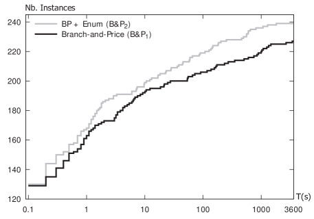
Figure 1: Number of instances solved over time by B&P₁ and B&P₂

Figure 1 displays the number of instances solved by B&P₁ and B&P₂ as a function of the CPU time limit. B&P₂ visibly produces superior results, but this method is also less flexible: its performance depends on the ability to do a complete route enumeration at the root node within the optimality gap. This process may possibly fail (due to time or memory limitations, or an unusually large gap), such that we recommend to first consider B&P₁ in exploratory analyses without any prior knowledge of the structure of the ITSRSP instances.

5.2 Heuristic solutions

As seen in the previous section, our exact methods can solve the majority of the instances, but their CPU time can widely vary, even for instances with similar characteristics. Therefore, fast heuristic solutions remain essential for applications requiring a response in a guaranteed short time. This section compares the performance of our HGS with that of the existing ITSRSP heuristics from Hemmati et al. (2014) and Hemmati and Hvattum (2016). To highlight the impact of the SP component, we evaluated two versions of our algorithm: without SP (HGS₁) and with SP (HGS₂).

We used the same parameters as Vidal et al. (2013) to avoid any problem-specific overfit. Therefore, $(\mu^{\textsc{min}},\mu^{\textsc{gen}})=(25,40)$, $\mu^{\textsc{elite}}=10$, $\mu^{\textsc{close}}=5$, $p_{\textsc{rep}}=0.5$, $\xi^{\textsc{ref}}=0.2$, $|\Gamma|=30$, and $(\gamma^{\textsc{tw}},\gamma^{\textsc{wt}})=(1.0,0.2)$. The penalty coefficients take $(\omega^{\textsc{q}},\omega^{\textsc{tw}},\omega^{I})=(\bar{c}/\bar{q},100,\bar{c})$ as a starting value, where $\bar{c}=\frac{\sum_{k\in K}\sum_{(i,j)\in A}c^{k}_{ij}}{|K||A|}$ and $\bar{q}=\frac{\sum_{i\in V}|q_{i}|}{n}$. To compare with previous literature in similar CPU time, we set $(It_{\textsc{ni}},T_{\textsc{max}})=(2.5\cdot 10^{3},15\,\text{min})$, and $T^{\textsc{sp}}_{\textsc{max}}=30\,\text{s}$. Finally, the full load instances (FUN) require directs visits from pickup to delivery points, such that neighborhoods ${\mathcal{N}}_{1}$ and ${\mathcal{N}}_{2}$ can be disabled and neighborhood ${\mathcal{N}}_{3}$ is restricted to $\Delta=0$. In the neighborhood restrictions, $i\in D$ is the only possible candidate successor of $i-n$, and only a pickup node $j\in P$ can follow a delivery $i\in D$.

Table 3 compares the results of the ALNS of Hemmati et al. (2014) with those of HGS₁ and HGS₂. Each line gives average results over 10 runs for five instances with the same characteristics. Each column “Gap” reports the percentage gap of one method relative to the optimal solutions found in Section 5.1, column “T” gives the total CPU time in minutes, and column “T*” gives the attainment time (in minutes) needed to reach the final solution. For each instance class, the best gap is highlighted in boldface. The detailed results of Hemmati et al. (2014) were kindly provided by the authors, and our complete detailed results (per instance) are also available in the electronic companion of this paper, located at https://w1.cirrelt.ca/~vidalt/en/VRP-resources.html.

Table 3: Performance comparison – Metaheuristics

		Hemmati et al. (2014)			HGS1				HGS2
	Instances	Gap	T		Gap	T	T*		Gap	T	T*
SS-MUN	C7-V3	0.00	0.03		0.00	0.02	0.00		0.00	0.02	0.00
	C10-V3	0.00	0.04		0.00	0.04	0.00		0.00	0.04	0.00
	C15-V4	0.58	0.09		0.00	0.08	0.00		0.00	0.08	0.00
	C18-V5	0.51	0.13		0.07	0.12	0.02		0.02	0.13	0.03
	C22-V6	1.82	0.19		0.05	0.19	0.05		0.00	0.18	0.04
	C23-V13	0.58	0.25		0.13	0.25	0.09		0.00	0.23	0.07
	C30-V6	1.60	0.38		0.17	0.36	0.17		0.00	0.33	0.12
	C35-V7	1.92	0.54		0.81	0.51	0.26		0.03	0.54	0.27
	C60-V13	1.69	2.01		1.03	2.44	1.81		0.14	2.25	1.37
	C80-V20	2.45	4.13		1.79	5.21	4.09		0.03	3.84	2.44
	C100-V30	2.68	7.77		1.67	9.97	8.01		0.01	5.31	3.02
	C130-V40	2.57	16.95		2.28	13.84	11.87		0.02	12.43	8.39
	Overall	1.37	2.71		0.67	2.75	2.20		0.02	2.12	1.31
SS-FUN	C8-V3	0.00	0.03		0.00	0.01	0.00		0.00	0.01	0.00
	C11-V4	0.13	0.05		0.00	0.02	0.00		0.00	0.02	0.00
	C13-V5	0.07	0.07		0.00	0.02	0.00		0.00	0.02	0.00
	C16-V6	0.05	0.10		0.00	0.03	0.00		0.00	0.03	0.00
	C17-V13	0.01	0.14		0.00	0.04	0.00		0.00	0.05	0.00
	C20-V6	0.14	0.18		0.00	0.04	0.00		0.00	0.05	0.00
	C25-V7	0.22	0.27		0.00	0.07	0.02		0.00	0.07	0.01
	C35-V13	0.29	0.60		0.01	0.19	0.08		0.00	0.17	0.05
	C50-V20	0.52	1.38		0.22	0.67	0.43		0.00	0.43	0.15
	C70-V30	1.29	3.51		0.68	1.86	1.28		0.00	1.09	0.42
	C90-V40	1.45	6.98		0.70	3.90	2.83		0.00	1.93	0.76
	C100-V50	0.96	9.79		0.50	5.98	4.46		0.00	2.83	1.20
	Overall	0.43	1.93		0.18	1.07	0.76		0.00	0.56	0.22
DS-MUN	C7-V3	0.00	0.03		0.00	0.02	0.00		0.00	0.02	0.00
	C10-V3	0.01	0.04		0.00	0.04	0.00		0.00	0.04	0.00
	C15-V4	1.26	0.08		0.00	0.08	0.01		0.00	0.08	0.01
	C18-V5	0.47	0.13		0.00	0.12	0.01		0.00	0.12	0.01
	C22-V6	2.18	0.19		0.01	0.18	0.05		0.00	0.18	0.05
	C23-V13	0.12	0.24		0.02	0.19	0.05		0.00	0.20	0.04
	C30-V6	1.04	0.37		0.22	0.36	0.17		0.03	0.32	0.12
	C35-V7	1.08	0.51		0.14	0.53	0.28		0.00	0.44	0.17
	C60-V13	3.74	1.92		1.41	2.58	1.96		0.03	1.81	1.06
	C80-V20	3.10	4.26		1.61	5.69	4.58		0.04	3.56	2.20
	C100-V30	3.69	8.00		3.27	9.22	7.27		0.01	9.87	6.84
	C130-V40	5.18	17.47		5.08	13.66	11.64		0.09	14.81	12.88
	Overall	1.82	2.77		0.98	2.72	2.17		0.02	2.62	1.95
DS-FUN	C8-V3	0.00	0.03		0.00	0.01	0.00		0.00	0.01	0.00
	C11-V4	0.00	0.05		0.00	0.02	0.00		0.00	0.02	0.00
	C13-V5	0.00	0.06		0.00	0.02	0.00		0.00	0.04	0.00
	C16-V6	0.03	0.10		0.00	0.03	0.00		0.00	0.04	0.00
	C17-V13	0.00	0.13		0.00	0.05	0.00		0.00	0.05	0.00
	C20-V6	0.01	0.16		0.00	0.04	0.00		0.00	0.05	0.00
	C25-V7	0.41	0.26		0.00	0.07	0.01		0.00	0.07	0.01
	C35-V13	1.03	0.59		0.01	0.26	0.14		0.00	0.21	0.08
	C50-V20	0.61	1.41		0.23	0.71	0.46		0.00	0.45	0.17
	C70-V30	0.59	3.55		0.31	2.02	1.43		0.00	1.02	0.38
	C90-V40	1.10	7.01		0.44	4.27	3.16		0.00	2.20	1.00
	C100-V50	1.07	9.85		0.41	6.37	4.80		0.00	3.13	1.44
	Overall	0.41	1.93		0.12	1.16	0.83		0.00	0.61	0.26

As visible in the results of Table 3, both versions of the HGS largely outperform previous algorithms. HGS₂ obtains near-optimal solutions within an average gap of $0.01\%$, compared to $1.01\%$ for the ALNS. The full load instances are generally easier to solve than the mixed load instances since the problem simplifies. Moreover, the SP-based procedure largely contributes to the performance of the algorithm: contrary to intuition, it does not increase the overall CPU time, but even decreases it from $1.93$ min (HGS₁) to $1.48$ min (HGS₂) on average. Indeed, the SP helps to reach optimal solutions more quickly, such that the method only performs $It_{\textsc{ni}}$ additional iterations before reaching the termination criteria instead of gradually improving over a longer time. The effect is manifest when comparing the average attainment time of HGS₁ (T* $=1.49\,\text{min}$) with that of HGS₂ ($0.94\,\text{min}$). In a follow-up work, Hemmati and Hvattum (2016) investigated the impact of some design decisions and parameters of their ALNS and reported the results of six variants of their algorithm on a smaller subset of instances. Drawing a comparison with these methods leads to similar conclusions: HGS₂ largely outperforms these methods. For the sake of brevity, this comparison is presented in the electronic companion.

5.3 Sensitivity analyses

To highlight the role of each main strategy and parameter, we have conducted extensive sensitivity analyses with the B&P and HGS algorithms. We started with the standard configurations of each method (B&P₁, B&P₂ and HGS₂) and generated a number of alternative configurations by deactivating a component or modifying a single parameter to study its impact. The results of these analyses are presented in Tables 4–5. In Table 4, Column “Gap” represent the average gap, Column “T” reports the average CPU time in minutes, Column “Root” counts the number of instances for which the root node solution was completed, and Column “Opt” counts the number of optimal solutions found. By convention, failing to solve the root node gives a Gap of 100%. In Table 5, Column “Gap” refers to the average gap, and Columns “T” and “T*” represent the average CPU time and attainment time.

Table 4: Impact of some of the key components of the B&P

		FUN					MUN
		Gap	T	Root	Opt		Gap	T	Root	Opt
Standard (B&P1)		0.00	0.02	120	120		0.01	8.94	120	107
A. No Heuristic Pricing		0.00	0.02	120	120		0.02	11.20	120	103
B. No Strong Branching		0.00	1.09	120	118		0.06	17.54	120	86
C. No Preprocessing		0.00	0.03	120	120		6.76	15.10	112	95
D. No DSSR		0.00	0.04	120	120		25.02	19.27	90	84
Standard (B&P2)		0.00	0.01	120	120		0.00	1.74	120	119
E. No Completion Bounds		0.00	0.01	120	120		13.33	9.97	104	104
F. No Subset-Row Cuts		0.00	0.01	120	120		0.00	2.47	120	118

Table 5: Impact of some of the key components and parameters of the HGS

	FUN					MUN
	Gap	T	T*			Gap	T	T*
Standard (HGS2)	0.00	0.58	0.24			0.02	2.37	1.63
G. No SP Intensification (HGS1)	0.15	1.11	0.80			0.82	2.74	2.18
H. Shorter SP Intensification ($T^{\textsc{sp}}_{\textsc{max}}=10\,\text{s}$)	0.00	0.58	0.24			0.02	2.29	1.54
I. Longer SP Intensification ($T^{\textsc{sp}}_{\textsc{max}}=120\,\text{s}$)	0.00	0.58	0.24			0.02	2.37	1.59
J. No neighborhood restrictions ($|\Gamma|=+\infty$)	0.00	0.72	0.29			0.05	3.49	2.35
K. No diversity management ($f_{\mathcal{P}}^{\textsc{div}}(\cdot)=0$)	0.00	0.58	0.25			0.03	2.39	1.71

In these experiments, again, the instances of class FUN are solved more easily. Since most methods achieve the same solution quality for this class, we will primarily rely on the harder MUN instances in our analyses.

Table 4 analyzes the components of the B&P algorithms. As illustrated by the results of Configuration A, heuristic pricing significantly reduces the overall pricing time. Without this component, four additional instances remain open and the CPU time increases by 25%, though this effect is generally less marked than in other VRP variants (see, e.g. Desaulniers et al. 2008, Martinelli et al. 2014).

Deactivating strong branching (Configuration B) has a larger impact. Strong branching helps predicting good branching decisions and reducing the search tree. Without it, the number of solved instances decreases from 107 to 86. The method can still nearly close the optimality gap (0.06% on average), but it often fails to complete the optimality proof.

Configurations C and D evaluate the impact of our advanced preprocessing strategies and DSSR (Section 3.1). Both components focus on enhancing the speed of the DP pricing algorithm. These components play a decisive role. Deactivating just one of these components makes it impossible to compute the root-node relaxation in a reasonable time for many instances. As an immediate consequence, the number of optimal solutions dramatically decreases (down to 84/120) and the optimality gap soars (up to 25.02%) due to the number of incomplete root node calculations.

The remaining analyses of Table 4 concern the B&P₂ algorithm, based on route enumeration. In addition to the preprocessing strategies and DSSR, the DP algorithm used for route enumeration exploits a sophisticated succession of completion bounds (Section 3.3). Deactivating these bounds, as in Configuration E, hinders the performance of the route enumeration algorithm, which fails on 16/120 largest instances. Remark that any instance which is successfully enumerated is subsequently solved. Finally, deactivating the SRC separation is moderately detrimental: it leads to an 42% increase of CPU time and one additional open instance.

The results of the sensitivity analysis of the HGS, in Table 5, essentially highlight the importance of the SP-based intensification procedure. As visible in Configuration F, the solution quality of HGS significantly decreases (up to 0.82% average gap on the MUN instances) when this strategy is deactivated. HGS identifies the routes (columns) belonging to the optimal solutions within the available number of iterations, but due to the large number of ships, ship types, and the cargo-ship incompatibility matrix, combining these routes into a complete solution can be a challenging task. In contrast, the SP component is perfectly suited for this role, such that the combination of both techniques leads to a particularly effective matheuristic.

The impact of other components and parameter settings is less marked: increasing or decreasing the time limit of each SP model (Configurations H and I) does not impact the solution method, due to the fact that most SP models are solved within a few seconds. Moreover, deactivating our ship-dependent neighborhood restrictions (Configuration J) and population-diversity management strategies (Configuration K) leads to a small but significant decrease of solution quality.

5.4 Experiments on large-scale instances

Most shipping companies solve planning problems involving at most a few dozen ships per segment (Wilson 2018). Still, some scenarios may exceptionally require to consider larger instances, for example when evaluating possible merger or coordinated freight operations. Efficient optimization tools are needed to react in such situations. The goal of this section is to evaluate the scalability of our algorithms in such cases. For this analysis, we produced $32$ new instances with the same problem generator as Hemmati et al. (2014), with up to $89$ ships and $260$ cargoes (i.e., $520$ pickups and deliveries). These instances are accessible at https://w1.cirrelt.ca/~vidalt/en/VRP-resources.html. We apply the B&P₂ and the HGS₂ with the same parameters as previously, and increase the CPU-time limits by a factor of four. Therefore, the HGS₂ is run with $T_{\textsc{max}}=1\,\text{h}$ and $T^{\textsc{sp}}_{\textsc{max}}=2\,\text{min}$. Similarly, the B&P₂ is run until a time limit of four hours is exceeded. However, to obtain lower bounds for all instances, we do not interrupt the B&P₂ until it has at least completed the solution of the root node.

Table 6 reports the results of this experiment using the same conventions as Tables 2 and 3. For these instances, we could not obtain optimal solutions on all instances, such that the column “Gap” for the HGS₂ reports the gap relative to the best lower bound found by the B&P₂. In addition, detailed solution values for each instance are provided in the electronic companion.

Table 6: Performance on larger instances

		Branch-and-Price + Enumeration + SRCs (B&P2)											HGS2
	Instance	TE	RE	Gap0	T0	Cuts0	RF	GapF	TF	CutsF	NF		Gap	T	T*
SS-MUN	C143-V41	5.22	385K	0.13	20.39	44	143K	0.00	24.38	209	33		0.04	15.85	10.69
	C156-V45	7.40	1M	0.12	35.42	58	509K	0.00	71.98	502	129		0.01	28.15	18.19
	C169-V48	6.83	199K	0.06	39.08	53	88K	0.00	41.71	159	19		0.01	26.32	19.28
	C182-V52	13.22	762K	0.10	53.72	38	482K	0.00	88.32	406	101		0.03	42.22	31.34
	C195-V56	29.25	297K	0.06	133.40	71	180K	0.00	147.68	282	47		0.04	50.21	39.07
	C208-V59	57.49	8M	0.12	135.82	59	2M	0.02	240.00	625	157		0.03	56.17	46.63
	C221-V63‡	-	-	0.17	495.02	-	-	0.17	495.02	-	-		0.20	56.32	45.02
	C260-V74‡	-	-	0.17	1196.78	-	-	0.17	1196.78	-	-		0.25	60.16	53.57
	Overall	19.90	2M	0.10	69.64	53.8	559K	0.04	258.23	363.8	81.0		0.08	41.93	32.97
SS-FUN	C110-V52	0.01	2K	0.01	0.07	0	2K	0.00	0.14	0	3		0.00	4.01	1.88
	C120-V53	0.01	3K	0.01	0.10	4	3K	0.00	0.29	7	5		0.00	4.40	1.87
	C130-V58	0.01	4K	0.01	0.14	10	3K	0.00	0.35	22	5		0.00	5.58	2.67
	C140-V62	0.01	1K	0.00	0.14	0	1K	0.00	0.14	0	1		0.00	6.49	2.71
	C150-V67	0.02	4K	0.00	0.20	3	4K	0.00	0.34	3	3		0.00	7.66	3.33
	C160-V71	0.03	6K	0.01	0.32	5	6K	0.00	1.31	19	11		0.00	9.14	3.96
	C170-V76	0.03	2K	0.00	0.34	0	2K	0.00	0.34	0	1		0.00	13.05	6.95
	C200-V89	0.05	4K	0.00	0.78	0	4K	0.00	0.78	0	1		0.01	20.74	11.52
	Overall	0.02	3K	0.00	0.26	2.8	3K	0.00	0.46	6.4	3.8		0.00	8.88	4.36
DS-MUN	C143-V41	5.51	16M	0.39	11.63	78	8M	0.00	33.66	315	37		0.04	42.36	34.89
	C156-V45	1.14	102K	0.01	7.73	78	12K	0.00	8.09	78	3		0.04	43.33	34.79
	C169-V48†	-	-	0.35	240.00	-	-	0.35	240.00	-	-		0.40	55.06	47.54
	C182-V52†	-	-	0.51	240.00	-	-	0.51	240.00	-	-		0.60	57.21	49.01
	C195-V56†	-	-	0.44	240.00	-	-	0.44	240.00	-	-		0.62	57.95	49.53
	C208-V59†	-	-	1.28	240.00	-	-	1.28	240.00	-	-		1.50	56.32	47.13
	C221-V63‡	-	-	0.46	481.31	-	-	0.46	481.31	-	-		0.62	59.39	50.24
	C260-V74‡	-	-	1.04	3848.88	-	-	1.04	3848.88	-	-		1.32	60.00	52.28
	Overall	3.33	8M	0.20	9.68	78.0	4M	0.51	666.49	196.5	20.0		0.64	53.95	45.67
DS-FUN	C110-V52	0.01	2K	0.00	0.04	0	2K	0.00	0.04	0	1		0.00	3.72	1.40
	C120-V53	0.01	2K	0.00	0.06	5	2K	0.00	0.06	5	1		0.00	4.75	2.12
	C130-V58	0.02	2K	0.00	0.07	0	2K	0.00	0.07	0	1		0.00	5.70	2.54
	C140-V62	0.02	5K	0.00	0.12	0	5K	0.00	0.12	0	1		0.00	6.87	3.16
	C150-V67	0.03	17K	0.00	0.14	2	17K	0.00	0.96	14	9		0.00	8.35	3.97
	C160-V71	0.03	2K	0.00	0.15	0	2K	0.00	0.15	0	1		0.00	13.46	8.19
	C170-V76	0.03	12K	0.00	0.18	5	12K	0.00	0.39	5	3		0.00	14.74	8.32
	C200-V89	0.06	77K	0.00	0.45	9	77K	0.00	8.54	73	37		0.00	17.95	9.37
	Overall	0.03	15K	0.00	0.15	2.6	15K	0.00	1.29	12.1	6.8		0.00	9.44	4.88
$\dagger$ Root-node solution was completed within four hours but enumeration exceeded four hours, triggering termination.
$\ddagger$ Root-node solution exceeded four hours.

The results on the new large-scale instances are consistent with our previous findings. All the full load instances are solved to optimality within a few minutes. In contrast, the mixed load instances are significantly more difficult since the deliveries can occur in any position after their associated pickups. This leads to a larger search space which effectively requires to arrange up to 520 visits (i.e., 260 pickups and deliveries) in the largest case. Seven out of the $16$ large mixed load instances are solved to optimality. For the remaining $9$ instances, the optimality gap is always smaller than $1.28\%$, but the root-node solution took up to 64 hours in the largest case (DS-MUN-C260-V74). The solutions of the proposed heuristic are also remarkably accurate. For the full load instances, the HGS₂ always finds near-optimal solutions (average gap below $0.01\%$) in an average time of $9.16$ minutes. For the mixed load instances, the HGS₂ complements very well the exact method by producing consistently good solutions (average gap of $0.36\%$) within a controllable CPU time ($47.94$ minutes on average).

6 Conclusions and Perspectives

As demonstrated in this paper, the literature on maritime logistics has attained a turning point where state-of-the-art exact algorithms can solve industrial and tramp ship routing optimization problems of a realistic scale. The B&P algorithm that we designed for this purpose capitalizes on multiple methodological elements to find a good balance between relaxation strength and pricing speed. As demonstrated by our sensitivity analyses, its most critical method components concern the efficiency of the DP pricing and enumeration algorithms: our sophisticated preprocessing techniques and filters, the use of DSSR to reintroduce elementarity and the successive completion bounds are essential to solve large ITSRSPs instances. These observations are in line with the works of Pecin et al. (2017), Sadykov et al. (2017) and the general research on MIP for VRPs which, for a large part, focuses on finding tighter relaxations and faster DP algorithms.

From the heuristic viewpoint, our experiments with a problem-tailored HGS show that the routes of optimal solutions can usually be quickly identified, but that crossover and local search methods are easily tricked into suboptimal route selections. Hybridizing the HGS with an SP solver fixes this issue and allows to attain near-optimal solutions within minutes.

Overall, the algorithms presented in this paper have contributed to push the limits of performance and problem tractability, but multiple avenues of research remain open concerning model accuracy. Indeed, despite its relevance for maritime transportation companies, the ITSRSPs remains a mere simplification of reality. As highlighted in Christiansen and Fagerholt (2014), it does not consider load-dependent fuel consumption, possible load splitting and flexible cargo quantities, or the possibility of slow-steaming on selected route segments. Emission control areas and sea conditions (e.g. depth and currents) are also largely ignored. Last but not the least, considerable reductions of turnaround time may be achieved by jointly optimizing ship routing and port operations within integrated supply chains. Adapting state-of-the-art exact and heuristic algorithms to handle these complex attributes remain a significant challenge for the future.

7 Acknowledgements

This work was supported by the Conselho Nacional de Desenvolvimento Científico e Tecnológico (CNPq) under Grant numbers 308528/2018-2, 134795/2016-4, 425962/2016-4 and 313521/2017-4, and Fundação Carlos Chagas Filho de Amparo à Pesquisa do Estado do Rio de Janeiro (FAPERJ) under Grant number E-26/202.790/2019.

Appendix – Detailed Results

Tables 7 to 11 give the detailed results of B&P₂ and HGS₂ (with the set partitioning component) on each individual instance. For the B&P₂, Columns “Opt” and “T” represent the optimal value and the total CPU time (in minutes). For the HGS₂, Columns “Best”, “Avg” and “Worst” represent the best, average and worst cost found over $10$ runs. Column “T” gives the total CPU time in minutes, and column “T*” gives the attainment time (in minutes) needed to reach the final solution. In Table 11, Columns “LB” and “UB” represent the bounds found by the B&P₂.

Table 7: Results for short sea mixed load instances

Instance	B&P2			HGS2
	Opt	T		Best	Avg	Worst	T	T*
SHORTSEA_MUN_C7_V3_HE_1	1476444	0.00		1476444	1476444.0	1476444	0.02	0.00
SHORTSEA_MUN_C7_V3_HE_2	1134176	0.00		1134176	1134176.0	1134176	0.02	0.00
SHORTSEA_MUN_C7_V3_HE_3	1196466	0.00		1196466	1196466.0	1196466	0.02	0.00
SHORTSEA_MUN_C7_V3_HE_4	1256139	0.00		1256139	1256139.0	1256139	0.02	0.00
SHORTSEA_MUN_C7_V3_HE_5	1160394	0.00		1160394	1160394.0	1160394	0.02	0.00
SHORTSEA_MUN_C10_V3_HE_1	2083965	0.00		2083965	2083965.0	2083965	0.04	0.00
SHORTSEA_MUN_C10_V3_HE_2	2012364	0.00		2012364	2012364.0	2012364	0.04	0.00
SHORTSEA_MUN_C10_V3_HE_3	1986779	0.00		1986779	1986779.0	1986779	0.04	0.00
SHORTSEA_MUN_C10_V3_HE_4	2125461	0.00		2125461	2125461.0	2125461	0.04	0.00
SHORTSEA_MUN_C10_V3_HE_5	2162453	0.00		2162453	2162453.0	2162453	0.04	0.00
SHORTSEA_MUN_C15_V4_HE_1	1959153	0.00		1959153	1959153.0	1959153	0.08	0.00
SHORTSEA_MUN_C15_V4_HE_2	2560004	0.00		2560004	2560004.0	2560004	0.08	0.00
SHORTSEA_MUN_C15_V4_HE_3	2582912	0.00		2582912	2582912.0	2582912	0.08	0.01
SHORTSEA_MUN_C15_V4_HE_4	2265396	0.00		2265396	2265396.0	2265396	0.09	0.00
SHORTSEA_MUN_C15_V4_HE_5	2230861	0.00		2230861	2230861.0	2230861	0.08	0.00
SHORTSEA_MUN_C18_V5_HE_1	2374420	0.00		2374420	2374420.0	2374420	0.11	0.00
SHORTSEA_MUN_C18_V5_HE_2	2987358	0.00		2987358	2987358.0	2987358	0.11	0.01
SHORTSEA_MUN_C18_V5_HE_3	2301308	0.00		2301308	2301308.0	2301308	0.12	0.01
SHORTSEA_MUN_C18_V5_HE_4	2400016	0.00		2400016	2402999.2	2414932	0.16	0.05
SHORTSEA_MUN_C18_V5_HE_5	2813167	0.00		2813167	2813167.0	2813167	0.17	0.06
SHORTSEA_MUN_C22_V6_HE_1	3928483	0.00		3928483	3928483.0	3928483	0.17	0.03
SHORTSEA_MUN_C22_V6_HE_2	3683436	0.01		3683436	3683436.0	3683436	0.16	0.02
SHORTSEA_MUN_C22_V6_HE_3	3264770	0.00		3264770	3264770.0	3264770	0.18	0.04
SHORTSEA_MUN_C22_V6_HE_4	3228262	0.00		3228262	3228262.0	3228262	0.22	0.07
SHORTSEA_MUN_C22_V6_HE_5	3770560	0.00		3770560	3770560.0	3770560	0.17	0.03
SHORTSEA_MUN_C23_V13_HE_1	2276832	0.01		2276832	2276832.0	2276832	0.22	0.04
SHORTSEA_MUN_C23_V13_HE_2	2255469	0.01		2255469	2255469.0	2255469	0.22	0.06
SHORTSEA_MUN_C23_V13_HE_3	2362503	0.00		2362503	2362503.0	2362503	0.23	0.08
SHORTSEA_MUN_C23_V13_HE_4	2250110	0.02		2250110	2250110.0	2250110	0.25	0.08
SHORTSEA_MUN_C23_V13_HE_5	2325941	0.00		2325941	2325941.0	2325941	0.22	0.06
SHORTSEA_MUN_C30_V6_HE_1	4958542	0.00		4958542	4958542.0	4958542	0.31	0.10
SHORTSEA_MUN_C30_V6_HE_2	4549708	0.01		4549708	4549708.0	4549708	0.34	0.13
SHORTSEA_MUN_C30_V6_HE_3	4098111	0.02		4098111	4098111.0	4098111	0.33	0.11
SHORTSEA_MUN_C30_V6_HE_4	4449449	0.02		4449449	4449485.3	4449812	0.36	0.15
SHORTSEA_MUN_C30_V6_HE_5	4528514	0.01		4528514	4528514.0	4528514	0.29	0.09
SHORTSEA_MUN_C35_V7_HE_1	4893734	0.03		4893734	4898167.9	4913975	0.59	0.32
SHORTSEA_MUN_C35_V7_HE_2	4533265	0.21		4533265	4534290.3	4543518	0.53	0.23
SHORTSEA_MUN_C35_V7_HE_3	4433847	0.03		4433847	4433847.0	4433847	0.46	0.20
SHORTSEA_MUN_C35_V7_HE_4	4580935	0.05		4580935	4580935.0	4580935	0.51	0.23
SHORTSEA_MUN_C35_V7_HE_5	5511661	0.01		5511661	5513388.5	5523201	0.61	0.35
SHORTSEA_MUN_C60_V13_HE_1	8133385	0.96		8133385	8147210.5	8163045	2.71	1.70
SHORTSEA_MUN_C60_V13_HE_2	7971476	0.88		7971476	7972935.0	7984871	1.84	1.05
SHORTSEA_MUN_C60_V13_HE_3	7604198	0.75		7604198	7632301.3	7647547	2.56	1.74
SHORTSEA_MUN_C60_V13_HE_4	8505125	0.87		8505125	8505971.4	8508321	2.09	1.24
SHORTSEA_MUN_C60_V13_HE_5	8921750	1.08		8921750	8931617.8	8942531	2.08	1.11
SHORTSEA_MUN_C80_V20_HE_1	10289573	1.67		10289573	10294261.3	10305785	5.04	3.37
SHORTSEA_MUN_C80_V20_HE_2	10240618	0.91		10240618	10241641.4	10246354	3.64	2.32
SHORTSEA_MUN_C80_V20_HE_3	9606530	2.84		9606530	9606573.1	9606961	2.91	1.66
SHORTSEA_MUN_C80_V20_HE_4	11302476	0.45		11302476	11311027.3	11333280	4.78	3.21
SHORTSEA_MUN_C80_V20_HE_5	10862563	0.31		10862563	10863032.1	10867254	2.85	1.63
SHORTSEA_MUN_C100_V30_HE_1	12626988	2.53		12626988	12627601.8	12633126	4.59	2.48
SHORTSEA_MUN_C100_V30_HE_2	12774864	2.98		12774864	12775622.5	12776760	5.80	3.23
SHORTSEA_MUN_C100_V30_HE_3	11935332	7.82		11935332	11935349.0	11935502	5.14	2.92
SHORTSEA_MUN_C100_V30_HE_4	13605352	1.82		13605352	13610213.4	13612134	5.20	2.96
SHORTSEA_MUN_C100_V30_HE_5	13240648	1.20		13240648	13241314.4	13244485	5.83	3.54
SHORTSEA_MUN_C130_V40_HE_1	16316051	13.45		16316388	16318378.8	16319526	13.31	8.71
SHORTSEA_MUN_C130_V40_HE_2	16260579	27.23		16260579	16263866.0	16272543	12.64	8.63
SHORTSEA_MUN_C130_V40_HE_3	15537963	17.97		15537963	15543747.8	15551928	12.68	9.03
SHORTSEA_MUN_C130_V40_HE_4	17011065	6.65		17011065	17012795.2	17014853	11.82	7.84
SHORTSEA_MUN_C130_V40_HE_5	18273893	10.11		18273893	18275423.4	18281922	11.71	7.75

Table 8: Results for short sea full load instances

Instance	B&P2			HGS2
	Opt	T		Best	Avg	Worst	T	T*
SHORTSEA_FUN_C8_V3_HE_1	1391997	0.00		1391997	1391997.0	1391997	0.01	0.00
SHORTSEA_FUN_C8_V3_HE_2	1246273	0.00		1246273	1246273.0	1246273	0.01	0.00
SHORTSEA_FUN_C8_V3_HE_3	1698102	0.00		1698102	1698102.0	1698102	0.01	0.00
SHORTSEA_FUN_C8_V3_HE_4	1777637	0.00		1777637	1777637.0	1777637	0.01	0.00
SHORTSEA_FUN_C8_V3_HE_5	1636788	0.00		1636788	1636788.0	1636788	0.01	0.00
SHORTSEA_FUN_C11_V4_HE_1	1052463	0.00		1052463	1052463.0	1052463	0.02	0.00
SHORTSEA_FUN_C11_V4_HE_2	1067139	0.00		1067139	1067139.0	1067139	0.02	0.00
SHORTSEA_FUN_C11_V4_HE_3	1212388	0.00		1212388	1212388.0	1212388	0.02	0.00
SHORTSEA_FUN_C11_V4_HE_4	1185465	0.00		1185465	1185465.0	1185465	0.02	0.00
SHORTSEA_FUN_C11_V4_HE_5	1310285	0.00		1310285	1310285.0	1310285	0.02	0.00
SHORTSEA_FUN_C13_V5_HE_1	2034184	0.00		2034184	2034184.0	2034184	0.02	0.00
SHORTSEA_FUN_C13_V5_HE_2	2043253	0.00		2043253	2043253.0	2043253	0.03	0.00
SHORTSEA_FUN_C13_V5_HE_3	2378283	0.00		2378283	2378283.0	2378283	0.03	0.00
SHORTSEA_FUN_C13_V5_HE_4	2707215	0.00		2707215	2707215.0	2707215	0.02	0.00
SHORTSEA_FUN_C13_V5_HE_5	3011648	0.00		3011648	3011648.0	3011648	0.02	0.00
SHORTSEA_FUN_C16_V6_HE_1	3577005	0.00		3577005	3577005.0	3577005	0.03	0.00
SHORTSEA_FUN_C16_V6_HE_2	3560203	0.00		3560203	3560203.0	3560203	0.03	0.00
SHORTSEA_FUN_C16_V6_HE_3	4081013	0.00		4081013	4081013.0	4081013	0.04	0.00
SHORTSEA_FUN_C16_V6_HE_4	3667080	0.00		3667080	3667080.0	3667080	0.03	0.00
SHORTSEA_FUN_C16_V6_HE_5	3438493	0.00		3438493	3438493.0	3438493	0.03	0.00
SHORTSEA_FUN_C17_V13_HE_1	2265731	0.00		2265731	2265731.0	2265731	0.05	0.00
SHORTSEA_FUN_C17_V13_HE_2	3154165	0.00		3154165	3154165.0	3154165	0.05	0.00
SHORTSEA_FUN_C17_V13_HE_3	2699378	0.00		2699378	2699378.0	2699378	0.06	0.01
SHORTSEA_FUN_C17_V13_HE_4	2806231	0.00		2806231	2806231.0	2806231	0.05	0.00
SHORTSEA_FUN_C17_V13_HE_5	2910814	0.00		2910814	2910814.0	2910814	0.05	0.00
SHORTSEA_FUN_C20_V6_HE_1	2973381	0.00		2973381	2973381.0	2973381	0.05	0.00
SHORTSEA_FUN_C20_V6_HE_2	3206514	0.00		3206514	3206514.0	3206514	0.05	0.01
SHORTSEA_FUN_C20_V6_HE_3	3197445	0.00		3197445	3197445.0	3197445	0.05	0.01
SHORTSEA_FUN_C20_V6_HE_4	3342130	0.00		3342130	3342130.0	3342130	0.05	0.00
SHORTSEA_FUN_C20_V6_HE_5	3156378	0.00		3156378	3156378.0	3156378	0.05	0.00
SHORTSEA_FUN_C25_V7_HE_1	3833588	0.00		3833588	3833588.0	3833588	0.07	0.02
SHORTSEA_FUN_C25_V7_HE_2	3673666	0.00		3673666	3673666.0	3673666	0.07	0.01
SHORTSEA_FUN_C25_V7_HE_3	4238213	0.00		4238213	4238213.0	4238213	0.07	0.01
SHORTSEA_FUN_C25_V7_HE_4	4260762	0.00		4260762	4260762.0	4260762	0.08	0.02
SHORTSEA_FUN_C25_V7_HE_5	4069693	0.00		4069693	4069693.0	4069693	0.08	0.02
SHORTSEA_FUN_C35_V13_HE_1	2986667	0.00		2986667	2986667.0	2986667	0.14	0.02
SHORTSEA_FUN_C35_V13_HE_2	3002973	0.00		3002973	3002973.0	3002973	0.20	0.07
SHORTSEA_FUN_C35_V13_HE_3	3084339	0.00		3084339	3084339.0	3084339	0.16	0.04
SHORTSEA_FUN_C35_V13_HE_4	3952461	0.00		3952461	3952461.0	3952461	0.18	0.06
SHORTSEA_FUN_C35_V13_HE_5	3293086	0.00		3293086	3293086.0	3293086	0.18	0.06
SHORTSEA_FUN_C50_V20_HE_1	7258266	0.00		7258266	7258266.0	7258266	0.40	0.13
SHORTSEA_FUN_C50_V20_HE_2	7452465	0.01		7452465	7452465.0	7452465	0.44	0.17
SHORTSEA_FUN_C50_V20_HE_3	6922293	0.01		6922293	6922293.0	6922293	0.44	0.15
SHORTSEA_FUN_C50_V20_HE_4	8933846	0.01		8933846	8933846.5	8933848	0.46	0.17
SHORTSEA_FUN_C50_V20_HE_5	7322307	0.01		7322307	7322307.0	7322307	0.40	0.13
SHORTSEA_FUN_C70_V30_HE_1	10051856	0.02		10051856	10051856.0	10051856	0.98	0.39
SHORTSEA_FUN_C70_V30_HE_2	10455468	0.01		10455468	10455468.0	10455468	0.99	0.38
SHORTSEA_FUN_C70_V30_HE_3	10172541	0.01		10172541	10172541.0	10172541	1.27	0.62
SHORTSEA_FUN_C70_V30_HE_4	10854036	0.06		10854036	10854036.0	10854036	1.02	0.38
SHORTSEA_FUN_C70_V30_HE_5	10886838	0.10		10886838	10886838.0	10886838	1.16	0.35
SHORTSEA_FUN_C90_V40_HE_1	13361947	0.03		13361947	13362943.0	13371155	1.94	0.82
SHORTSEA_FUN_C90_V40_HE_2	13828112	0.02		13828112	13828112.0	13828112	1.88	0.71
SHORTSEA_FUN_C90_V40_HE_3	12627125	0.08		12627125	12627476.1	12628003	1.77	0.63
SHORTSEA_FUN_C90_V40_HE_4	14406428	0.03		14406428	14406689.8	14409031	1.82	0.64
SHORTSEA_FUN_C90_V40_HE_5	13560830	0.06		13560830	13560835.3	13560853	2.23	1.01
SHORTSEA_FUN_C100_V50_HE_1	13800823	0.03		13800823	13800823.0	13800823	2.94	1.35
SHORTSEA_FUN_C100_V50_HE_2	14644836	0.19		14644836	14645381.1	14647299	3.02	1.30
SHORTSEA_FUN_C100_V50_HE_3	13135505	0.05		13135505	13135756.6	13136396	2.65	1.02
SHORTSEA_FUN_C100_V50_HE_4	14841840	0.14		14841840	14841840.4	14841841	3.06	1.41
SHORTSEA_FUN_C100_V50_HE_5	14009874	0.07		14009874	14009971.3	14010827	2.48	0.93

Table 9: Results for deep sea mixed load instances

Instance	B&P2			HGS2
	Opt	T		Best	Avg	Worst	T	T*
DEEPSEA_MUN_C7_V3_HE_1	5233464	0.00		5233464	5233464.0	5233464	0.02	0.00
DEEPSEA_MUN_C7_V3_HE_2	6053699	0.00		6053699	6053699.0	6053699	0.02	0.00
DEEPSEA_MUN_C7_V3_HE_3	5888949	0.00		5888949	5888949.0	5888949	0.02	0.00
DEEPSEA_MUN_C7_V3_HE_4	6510656	0.00		6510656	6510656.0	6510656	0.02	0.00
DEEPSEA_MUN_C7_V3_HE_5	7220458	0.00		7220458	7220458.0	7220458	0.02	0.00
DEEPSEA_MUN_C10_V3_HE_1	7986248	0.00		7986248	7986248.0	7986248	0.04	0.00
DEEPSEA_MUN_C10_V3_HE_2	7754484	0.00		7754484	7754484.0	7754484	0.04	0.00
DEEPSEA_MUN_C10_V3_HE_3	9499357	0.00		9499357	9499357.0	9499357	0.04	0.00
DEEPSEA_MUN_C10_V3_HE_4	8617192	0.00		8617192	8617192.0	8617192	0.04	0.00
DEEPSEA_MUN_C10_V3_HE_5	8653992	0.00		8653992	8653992.0	8653992	0.04	0.00
DEEPSEA_MUN_C15_V4_HE_1	13467090	0.00		13467090	13467090.0	13467090	0.07	0.00
DEEPSEA_MUN_C15_V4_HE_2	12457251	0.00		12457251	12457251.0	12457251	0.10	0.02
DEEPSEA_MUN_C15_V4_HE_3	12567396	0.00		12567396	12567396.0	12567396	0.08	0.00
DEEPSEA_MUN_C15_V4_HE_4	11764241	0.00		11764241	11764241.0	11764241	0.08	0.01
DEEPSEA_MUN_C15_V4_HE_5	10833640	0.00		10833640	10833640.0	10833640	0.08	0.00
DEEPSEA_MUN_C18_V5_HE_1	43054055	0.00		43054055	43054055.0	43054055	0.14	0.02
DEEPSEA_MUN_C18_V5_HE_2	25068287	0.00		25068287	25068287.0	25068287	0.13	0.02
DEEPSEA_MUN_C18_V5_HE_3	29211238	0.00		29211238	29211238.0	29211238	0.12	0.00
DEEPSEA_MUN_C18_V5_HE_4	32281904	0.00		32281904	32281904.0	32281904	0.11	0.00
DEEPSEA_MUN_C18_V5_HE_5	40718028	0.00		40718028	40718028.0	40718028	0.12	0.02
DEEPSEA_MUN_C22_V6_HE_1	41176718	0.00		41176718	41176718.0	41176718	0.16	0.03
DEEPSEA_MUN_C22_V6_HE_2	37236363	0.00		37236363	37236363.0	37236363	0.17	0.05
DEEPSEA_MUN_C22_V6_HE_3	38215238	0.00		38215238	38215238.0	38215238	0.17	0.03
DEEPSEA_MUN_C22_V6_HE_4	34129809	0.00		34129809	34129809.0	34129809	0.22	0.08
DEEPSEA_MUN_C22_V6_HE_5	46379332	0.00		46379332	46379332.0	46379332	0.17	0.04
DEEPSEA_MUN_C23_V13_HE_1	41002992	0.00		41002992	41002992.0	41002992	0.19	0.04
DEEPSEA_MUN_C23_V13_HE_2	28014147	0.00		28014147	28014147.0	28014147	0.19	0.02
DEEPSEA_MUN_C23_V13_HE_3	29090422	0.00		29090422	29090422.0	29090422	0.17	0.00
DEEPSEA_MUN_C23_V13_HE_4	33685274	0.00		33685274	33685274.0	33685274	0.23	0.07
DEEPSEA_MUN_C23_V13_HE_5	38664843	0.00		38664843	38664843.0	38664843	0.20	0.06
DEEPSEA_MUN_C30_V6_HE_1	19227093	0.00		19227093	19227093.0	19227093	0.31	0.12
DEEPSEA_MUN_C30_V6_HE_2	16784810	0.02		16784810	16784810.0	16784810	0.35	0.11
DEEPSEA_MUN_C30_V6_HE_3	21183928	0.01		21183928	21213100.9	21298546	0.35	0.16
DEEPSEA_MUN_C30_V6_HE_4	21076728	0.00		21076728	21076728.0	21076728	0.28	0.09
DEEPSEA_MUN_C30_V6_HE_5	24490671	0.01		24490671	24490671.0	24490671	0.33	0.12
DEEPSEA_MUN_C35_V7_HE_1	65082675	0.01		65082675	65086315.3	65119078	0.50	0.21
DEEPSEA_MUN_C35_V7_HE_2	54810586	0.03		54810586	54810586.0	54810586	0.45	0.18
DEEPSEA_MUN_C35_V7_HE_3	56182502	0.00		56182502	56182502.0	56182502	0.42	0.14
DEEPSEA_MUN_C35_V7_HE_4	61354812	0.02		61354812	61354812.0	61354812	0.46	0.16
DEEPSEA_MUN_C35_V7_HE_5	63904705	0.00		63904705	63904705.0	63904705	0.39	0.15
DEEPSEA_MUN_C60_V13_HE_1	80649895	3.25		80649895	80696507.0	80708160	2.13	1.14
DEEPSEA_MUN_C60_V13_HE_2	74881109	0.10		74881109	74881109.4	74881110	1.86	1.21
DEEPSEA_MUN_C60_V13_HE_3	91766747	0.03		91766747	91768529.1	91782830	1.47	0.78
DEEPSEA_MUN_C60_V13_HE_4	89702352	0.05		89702352	89763856.0	89863541	1.90	1.17
DEEPSEA_MUN_C60_V13_HE_5	88486544	0.08		88486544	88498544.6	88606550	1.71	1.00
DEEPSEA_MUN_C80_V20_HE_1	70718084	0.33		70718084	70799785.6	70922338	3.20	1.78
DEEPSEA_MUN_C80_V20_HE_2	73558165	1.95		73558165	73589043.3	73603212	5.07	3.47
DEEPSEA_MUN_C80_V20_HE_3	78250612	0.12		78250612	78251002.0	78254512	2.56	1.43
DEEPSEA_MUN_C80_V20_HE_4	75962439	0.32		75962439	75994306.3	76061556	3.67	2.34
DEEPSEA_MUN_C80_V20_HE_5	74162521	0.22		74162521	74169783.2	74207930	3.29	1.97
DEEPSEA_MUN_C100_V30_HE_1	150481912	1.25		150481912	150508649.2	150525751	10.03	7.17
DEEPSEA_MUN_C100_V30_HE_2	150826322	0.52		150826322	150834992.9	150866157	12.08	9.54
DEEPSEA_MUN_C100_V30_HE_3	151027805	1.83		151027805	151036770.9	151039246	8.58	4.48
DEEPSEA_MUN_C100_V30_HE_4	151193009	6.33		151193009	151218563.7	151331951	10.65	7.34
DEEPSEA_MUN_C100_V30_HE_5	159789021	0.75		159789021	159799748.9	159828402	8.02	5.67
DEEPSEA_MUN_C130_V40_HE_1	232582224	5.30		232625726	232672618.6	232835502	14.74	12.29
DEEPSEA_MUN_C130_V40_HE_2	228036360	265.06		228205988	228285255.3	228365518	15.00	13.56
DEEPSEA_MUN_C130_V40_HE_3	235657072	9.49		235666249	235772248.0	236033885	15.00	13.66
DEEPSEA_MUN_C130_V40_HE_4	220357686	6.40		220360711	220564140.8	220783879	14.31	11.66
DEEPSEA_MUN_C130_V40_HE_5	235381937	7.03		235487434	235739525.3	235849521	15.01	13.23

Table 10: Results for deep sea full load instances

Instance	B&P2			HGS2
	Opt	T		Best	Avg	Worst	T	T*
DEEPSEA_FUN_C8_V3_HE_1	9584863	0.00		9584863	9584863.0	9584863	0.01	0.00
DEEPSEA_FUN_C8_V3_HE_2	9369654	0.00		9369654	9369654.0	9369654	0.01	0.00
DEEPSEA_FUN_C8_V3_HE_3	4596681	0.00		4596681	4596681.0	4596681	0.01	0.00
DEEPSEA_FUN_C8_V3_HE_4	6899730	0.00		6899730	6899730.0	6899730	0.01	0.00
DEEPSEA_FUN_C8_V3_HE_5	6815253	0.00		6815253	6815253.0	6815253	0.01	0.00
DEEPSEA_FUN_C11_V4_HE_1	34854819	0.00		34854819	34854819.0	34854819	0.02	0.00
DEEPSEA_FUN_C11_V4_HE_2	25454434	0.00		25454434	25454434.0	25454434	0.02	0.00
DEEPSEA_FUN_C11_V4_HE_3	29627143	0.00		29627143	29627143.0	29627143	0.02	0.00
DEEPSEA_FUN_C11_V4_HE_4	33111680	0.00		33111680	33111680.0	33111680	0.02	0.00
DEEPSEA_FUN_C11_V4_HE_5	28175914	0.00		28175914	28175914.0	28175914	0.03	0.00
DEEPSEA_FUN_C13_V5_HE_1	11629005	0.00		11629005	11629005.0	11629005	0.04	0.00
DEEPSEA_FUN_C13_V5_HE_2	11820655	0.00		11820655	11820655.0	11820655	0.04	0.00
DEEPSEA_FUN_C13_V5_HE_3	9992593	0.00		9992593	9992593.0	9992593	0.04	0.00
DEEPSEA_FUN_C13_V5_HE_4	12819619	0.00		12819619	12819619.0	12819619	0.03	0.00
DEEPSEA_FUN_C13_V5_HE_5	10534892	0.00		10534892	10534892.0	10534892	0.03	0.00
DEEPSEA_FUN_C16_V6_HE_1	51127590	0.00		51127590	51127590.0	51127590	0.04	0.00
DEEPSEA_FUN_C16_V6_HE_2	44342796	0.00		44342796	44342796.0	44342796	0.03	0.00
DEEPSEA_FUN_C16_V6_HE_3	45391842	0.00		45391842	45391842.0	45391842	0.03	0.00
DEEPSEA_FUN_C16_V6_HE_4	39687114	0.00		39687114	39687114.0	39687114	0.04	0.00
DEEPSEA_FUN_C16_V6_HE_5	42855603	0.00		42855603	42855603.0	42855603	0.04	0.00
DEEPSEA_FUN_C17_V13_HE_1	17316720	0.00		17316720	17316720.0	17316720	0.04	0.00
DEEPSEA_FUN_C17_V13_HE_2	12194861	0.00		12194861	12194861.0	12194861	0.05	0.00
DEEPSEA_FUN_C17_V13_HE_3	12091554	0.00		12091554	12091554.0	12091554	0.05	0.00
DEEPSEA_FUN_C17_V13_HE_4	12847653	0.00		12847653	12847653.0	12847653	0.05	0.01
DEEPSEA_FUN_C17_V13_HE_5	13213406	0.00		13213406	13213406.0	13213406	0.05	0.00
DEEPSEA_FUN_C20_V6_HE_1	16406738	0.00		16406738	16406738.0	16406738	0.05	0.00
DEEPSEA_FUN_C20_V6_HE_2	16079401	0.00		16079401	16079401.0	16079401	0.05	0.00
DEEPSEA_FUN_C20_V6_HE_3	17342200	0.00		17342200	17342200.0	17342200	0.04	0.00
DEEPSEA_FUN_C20_V6_HE_4	16529748	0.00		16529748	16529748.0	16529748	0.05	0.01
DEEPSEA_FUN_C20_V6_HE_5	17449378	0.00		17449378	17449378.0	17449378	0.05	0.00
DEEPSEA_FUN_C25_V7_HE_1	22773158	0.00		22773158	22773158.0	22773158	0.07	0.01
DEEPSEA_FUN_C25_V7_HE_2	20206329	0.00		20206329	20206329.0	20206329	0.08	0.01
DEEPSEA_FUN_C25_V7_HE_3	19108952	0.00		19108952	19108952.0	19108952	0.07	0.01
DEEPSEA_FUN_C25_V7_HE_4	22668675	0.00		22668675	22668675.0	22668675	0.07	0.01
DEEPSEA_FUN_C25_V7_HE_5	23036603	0.00		23036603	23036603.0	23036603	0.08	0.02
DEEPSEA_FUN_C35_V13_HE_1	86951609	0.00		86951609	86951609.0	86951609	0.22	0.09
DEEPSEA_FUN_C35_V13_HE_2	83422071	0.00		83422071	83422071.0	83422071	0.19	0.07
DEEPSEA_FUN_C35_V13_HE_3	83898591	0.00		83898591	83898591.0	83898591	0.21	0.08
DEEPSEA_FUN_C35_V13_HE_4	91970481	0.00		91970481	91970481.0	91970481	0.23	0.09
DEEPSEA_FUN_C35_V13_HE_5	91123040	0.00		91123040	91123040.0	91123040	0.20	0.07
DEEPSEA_FUN_C50_V20_HE_1	41310946	0.00		41310946	41310946.0	41310946	0.46	0.18
DEEPSEA_FUN_C50_V20_HE_2	37784994	0.00		37784994	37784994.0	37784994	0.46	0.18
DEEPSEA_FUN_C50_V20_HE_3	39841724	0.00		39841724	39841724.0	39841724	0.41	0.13
DEEPSEA_FUN_C50_V20_HE_4	43941098	0.00		43941098	43941098.0	43941098	0.47	0.20
DEEPSEA_FUN_C50_V20_HE_5	41947437	0.00		41947437	41947437.0	41947437	0.46	0.18
DEEPSEA_FUN_C70_V30_HE_1	142679953	0.01		142679953	142679953.0	142679953	1.03	0.38
DEEPSEA_FUN_C70_V30_HE_2	135031988	0.02		135031988	135031988.0	135031988	1.06	0.36
DEEPSEA_FUN_C70_V30_HE_3	162759203	0.01		162759203	162759203.0	162759203	1.02	0.40
DEEPSEA_FUN_C70_V30_HE_4	155855123	0.01		155855123	155855123.0	155855123	1.06	0.44
DEEPSEA_FUN_C70_V30_HE_5	156557723	0.01		156557723	156557723.0	156557723	0.95	0.35
DEEPSEA_FUN_C90_V40_HE_1	190627186	0.06		190627186	190630992.5	190641592	2.08	0.83
DEEPSEA_FUN_C90_V40_HE_2	189770977	0.02		189770977	189771678.3	189777990	2.63	1.45
DEEPSEA_FUN_C90_V40_HE_3	211038412	0.02		211038412	211038684.4	211041136	2.15	0.94
DEEPSEA_FUN_C90_V40_HE_4	210449287	0.02		210449287	210449654.6	210451528	2.02	0.93
DEEPSEA_FUN_C90_V40_HE_5	197804917	0.05		197804917	197805398.0	197809727	2.11	0.87
DEEPSEA_FUN_C100_V50_HE_1	205826535	0.08		205826535	205831890.5	205844919	2.96	1.24
DEEPSEA_FUN_C100_V50_HE_2	207809147	0.03		207809147	207813969.7	207833395	4.33	2.62
DEEPSEA_FUN_C100_V50_HE_3	217000928	0.02		217000928	217000928.0	217000928	3.08	1.41
DEEPSEA_FUN_C100_V50_HE_4	220879632	0.03		220879632	220879794.0	220880172	2.49	0.83
DEEPSEA_FUN_C100_V50_HE_5	223265017	0.02		223265017	223265583.6	223270683	2.79	1.10

Table 11: Results for new large scale instances

Instance	B&P2				HGS2
	LB	UB	T		Best	Avg	Worst	T	T*
SHORTSEA_MUN_C143_V41	17799119.0	17799119	24.38		17804172	17806545.5	17810359	15.85	10.69
SHORTSEA_MUN_C156_V45	19342942.0	19342942	71.98		19343517	19344605.7	19346784	28.15	18.19
SHORTSEA_MUN_C169_V48	21268109.0	21268109	41.71		21268109	21270048.5	21278516	26.32	19.28
SHORTSEA_MUN_C182_V52	22980177.0	22980177	88.32		22982740	22986270.9	22991134	42.22	31.34
SHORTSEA_MUN_C195_V56	24440859.0	24440859	147.68		24440859	24450058.2	24468278	50.21	39.07
SHORTSEA_MUN_C208_V59	25708244.1	25712849	240.00		25712849	25716650.8	25723526	56.17	46.62
SHORTSEA_MUN_C221_V63	26989861.5	27034941	495.02		27034941	27042556.8	27058195	56.32	45.02
SHORTSEA_MUN_C260_V74	32407978.0	32464488	1196.78		32464488	32488515.1	32538633	60.16	53.57
SHORTSEA_FUN_C110_V52	15133771.0	15133771	0.14		15133771	15133926.9	15134691	4.01	1.88
SHORTSEA_FUN_C120_V53	16558958.0	16558958	0.29		16558993	16559104.9	16559264	4.40	1.87
SHORTSEA_FUN_C130_V58	17649436.0	17649436	0.35		17649436	17649659.7	17650377	5.58	2.67
SHORTSEA_FUN_C140_V62	19179026.0	19179026	0.14		19179026	19179026.2	19179027	6.49	2.71
SHORTSEA_FUN_C150_V67	20281407.0	20281407	0.34		20281407	20281794.0	20283296	7.65	3.33
SHORTSEA_FUN_C160_V71	21695647.0	21695647	1.31		21696335	21696659.8	21696858	9.14	3.96
SHORTSEA_FUN_C170_V76	23110481.0	23110481	0.34		23110481	23111291.2	23114048	13.06	6.95
SHORTSEA_FUN_C200_V89	27690324.0	27690324	0.78		27690324	27693029.9	27703323	20.74	11.52
DEEPSEA_MUN_C143_V41	254254590.0	254254590	33.66		254254591	254349635.7	254608621	42.36	34.89
DEEPSEA_MUN_C156_V45	270058045.0	270058045	8.09		270085318	270176938.6	270330689	43.32	34.79
DEEPSEA_MUN_C169_V48	289887680.2	290916269	240.00		290916269	291038620.0	291257150	55.06	47.54
DEEPSEA_MUN_C182_V52	300137926.8	301663875	240.00		301663875	301925296.5	302379995	57.21	49.01
DEEPSEA_MUN_C195_V56	310191451.9	311546377	240.00		311546377	312129552.3	313791486	57.95	49.53
DEEPSEA_MUN_C208_V59	341832426.9	346223133	240.00		346223133	346961721.4	347822705	56.32	47.13
DEEPSEA_MUN_C221_V63	350836918.3	352462189	481.31		352462189	352995236.0	354581124	59.39	50.24
DEEPSEA_MUN_C260_V74	404166031.4	408352976	3848.88		408352976	409513515.0	411652613	60.00	52.28
DEEPSEA_FUN_C110_V52	240011111.0	240011111	0.05		240011111	240014104.1	240026076	3.72	1.40
DEEPSEA_FUN_C120_V53	248614953.0	248614953	0.06		248614953	248618591.1	248633514	4.75	2.12
DEEPSEA_FUN_C130_V58	288771846.0	288771846	0.08		288771846	288771846.0	288771846	5.70	2.54
DEEPSEA_FUN_C140_V62	303231470.0	303231470	0.12		303231470	303231470.0	303231470	6.87	3.16
DEEPSEA_FUN_C150_V67	323442552.0	323442552	0.96		323442822	323455751.7	323466563	8.35	3.97
DEEPSEA_FUN_C160_V71	370429540.0	370429540	0.16		370429540	370439735.8	370471324	13.46	8.19
DEEPSEA_FUN_C170_V76	395641818.0	395641818	0.39		395641818	395648175.4	395663480	14.74	8.32
DEEPSEA_FUN_C200_V89	430966915.0	430966915	8.54		430970779	430984012.9	431008839	17.95	9.37

Appendix – Comparison with Hemmati and Hvattum (2016)

Hemmati and Hvattum (2016) have presented detailed results of six ALNS variants on a subset of the Hemmati et al. (2014) instances. Table 12 compares these results with those of HGS₂. Each line represents a group of instances, and the best results are highlighted in boldface. For each method, column “Gap” reports the percentage gap relative to the optimal solutions, and column “T” gives the total CPU time in minutes.

Table 12: Performance comparison with Hemmati and Hvattum (2016)

		ALNS1		ALNS2		ALNS3		ALNS4		ALNS5		ALNS6		HGS2
		Gap	T	Gap	T	Gap	T	Gap	T	Gap	T	Gap	T	Gap	T
SHORTSEA	C22-V6	0.29	0.18	0.29	0.20	0.23	0.19	0.17	0.19	0.35	0.20	0.53	0.18	0.00	0.18
	C23-V13	0.82	0.25	0.34	0.25	0.35	0.26	0.28	0.26	0.24	0.25	0.46	0.25	0.00	0.23
	C30-V6	1.32	0.35	0.66	0.40	1.14	0.41	0.90	0.42	1.04	0.39	1.95	0.38	0.00	0.33
	C35-V7	1.40	0.51	1.51	0.58	1.69	0.58	1.21	0.58	1.03	0.55	1.97	0.53	0.01	0.53
	C60-V13	2.89	2.05	2.29	2.18	2.83	2.29	2.30	2.42	2.63	2.06	1.81	1.95	0.13	2.14
	Overall	1.34	0.67	1.02	0.72	1.25	0.75	0.97	0.77	1.06	0.69	1.34	0.66	0.03	0.68
DEEPSEA	C22-V6	0.35	0.18	0.31	0.19	0.15	0.20	0.15	0.20	0.19	0.19	1.66	0.18	0.00	0.18
	C23-V13	0.00	0.26	0.00	0.26	0.02	0.28	0.01	0.28	0.00	0.25	0.00	0.24	0.00	0.20
	C30-V6	0.67	0.36	0.34	0.42	0.36	0.42	0.34	0.42	0.42	0.39	0.58	0.37	0.03	0.33
	C35-V7	0.61	0.52	0.51	0.60	0.50	0.60	0.58	0.63	0.37	0.54	0.69	0.51	0.00	0.43
	C60-V13	4.37	2.18	3.50	2.41	4.11	2.39	4.12	2.39	3.23	1.99	3.41	1.85	0.02	1.73
	Overall	1.20	0.70	0.93	0.78	1.03	0.78	1.04	0.78	0.84	0.67	1.27	0.63	0.01	0.57

References

- Andersson et al. (2011) Andersson, H., Christiansen, M., Fagerholt, K., 2011. The maritime pickup and delivery problem with time windows and split loads. INFOR: Information Systems and Operational Research 49, 79–91.
- Baldacci et al. (2011) Baldacci, R., Mingozzi, A., Roberti, R., 2011. New route relaxation and pricing strategies for the vehicle routing problem. Operations Research 59, 1269–1283.
- Bertsimas et al. (2019) Bertsimas, D., Jaillet, P., Martin, S., 2019. Online vehicle routing: The edge of optimization in large-scale applications. Operations Research 67, 143–162.
- Borthen et al. (2018) Borthen, T., Loennechen, H., Wang, X., Fagerholt, K., Vidal, T., 2018. A genetic search-based heuristic for a fleet size and periodic routing problem with application to offshore supply planning. EURO Journal on Transportation and Logistics 7, 121–150.
- Brønmo et al. (2007) Brønmo, G., Christiansen, M., Fagerholt, K., Nygreen, B., 2007. A multi-start local search heuristic for ship scheduling—a computational study. Computers & Operations Research 34, 900–917.
- Brown et al. (1987) Brown, G.G., Graves, G.W., Ronen, D., 1987. Scheduling ocean transportation of crude oil. Management Science 33, 335–346.
- Bulhões et al. (2018) Bulhões, T., Hà, M., Martinelli, R., Vidal, T., 2018. The vehicle routing problem with service level constraints. European Journal of Operational Research 265, 544–558.
- Christiansen and Fagerholt (2014) Christiansen, M., Fagerholt, K., 2014. Ship routing and scheduling in industrial and tramp shipping, in: Toth, P., Vigo, D. (Eds.), Vehicle Routing. Society for Industrial and Applied Mathematics, pp. 381–408.
- Christiansen et al. (2007) Christiansen, M., Fagerholt, K., Nygreen, B., Ronen, D., 2007. Maritime transportation, in: Barnhart, C., Laporte, G. (Eds.), Transportation. Elsevier, pp. 189–284.
- Christiansen et al. (2013) Christiansen, M., Fagerholt, K., Nygreen, B., Ronen, D., 2013. Ship routing and scheduling in the new millennium. European Journal of Operational Research 228, 467–483.
- Christofides et al. (1981) Christofides, N., Mingozzi, A., Toth, P., 1981. Exact algorithms for the vehicle routing problem, based on spanning tree and shortest path relaxations. Mathematical Programming 20, 255–282.
- Contardo and Martinelli (2014) Contardo, C., Martinelli, R., 2014. A new exact algorithm for the multi-depot vehicle routing problem under capacity and route length constraints. Discrete Optimization 12, 129–146.
- Desaulniers et al. (2008) Desaulniers, G., Lessard, F., Hadjar, A., 2008. Tabu search, partial elementarity, and generalized k-path inequalities for the vehicle routing problem with time windows. Transportation Science 42, 387–404.
- Duhamel et al. (2011) Duhamel, C., Lacomme, P., Prodhon, C., 2011. Efficient frameworks for greedy split and new depth first search split procedures for routing problems. Computers & Operations Research 38, 723–739.
- Dumas et al. (1991) Dumas, Y., Desrosiers, J., Soumis, F., 1991. The pickup and delivery problem with time windows. European Journal of Operational Research 54, 7–22.
- Fagerholt (2004) Fagerholt, K., 2004. A computer-based decision support system for vessel fleet scheduling - Experience and future research. Decision Support Systems 37, 35–47.
- Fagerholt and Christiansen (2000a) Fagerholt, K., Christiansen, M., 2000a. A combined ship scheduling and allocation problem. Journal of the Operational Research Society 51, 834–842.
- Fagerholt and Christiansen (2000b) Fagerholt, K., Christiansen, M., 2000b. A travelling salesman problem with allocation, time window and precedence constraints — an application to ship scheduling. International Transactions in Operational Research 7, 231–244.
- Glover and Hao (2009) Glover, F., Hao, J.K., 2009. The case for strategic oscillation. Annals of Operations Research 183, 163–173.
- Gschwind et al. (2018) Gschwind, T., Irnich, S., Rothenbächer, A.K., Tilk, C., 2018. Bidirectional labeling in column-generation algorithms for pickup-and-delivery problems. European Journal of Operational Research 266, 521–530.