A Mechanical Approach to One-Dimensional Interacting Gas

Abstract

Traditional derivations of the van der Waals equation typically use standard recipes involving ensemble averages of statistical mechanics. In this work, we study a box of weakly interacting gas particles in one-dimension from a purely mechanical point of view. This has the merit that it not only reproduces the van der Waals equation but also tells us some extra interesting physics not immediately clear from a pure statistical mechanical approach. For example, we find that the traditional handwaving interpretation of the van der Waals equation adopting mean field approximation is actually incorrect. In this investigation of one-dimensional interacting gas, we demonstrate the possibility taking a mechanical point of view and having deeper understanding for the physics of leading order effect of particle-particle interaction, for weakly interacting N-body systems that are usually studied in the framework of statistical mechanics or kinetic theory.

(This paper is the simplified version of the master thesis of Chung-Yang Wang at National Taiwan University.)

E-mail: chyawang@terpmail.umd.edu

1 Introduction

Statistical mechanics and kinetic theory are two main frameworks one adopts when studying a system containing a huge number of degrees of freedom. Researches in this field concern various systems, including hard sphere system [1, 2, 3, 4, 5, 6, 7, 8], hard ellipse system [9], hard needle system [10, 11], van der Waals theory [12, 13, 14, 15], granular particle system [16, 17, 18], etc. There are also researches concerning fundamental issues [19, 20].

Statistical mechanics and kinetic theory are powerful and systematic, but it often amounts to meaning that one has to pay the price of losing certain detailed dynamical information about the interparticular interactions. In order to study a weakly interacting N-body system, besides statistical mechanics, kinetic theory and numerical simulation, do we have other choice? At first glance, the idea of particle trajectory is useful only for systems containing small degrees of freedom. However, we can actually bring in the idea of trajectory for a N-body system if the effect of particle-particle interaction is weak. In this work, we study a weakly interacting one-dimensional gas to see how a direct approach investigating the detailed mechanical interaction between particles might shed some light on its merits as opposed to the traditional approach.

Before describing our mechanical approach, we first give a brief review of how one understands a weakly interacting one-dimensional gas in statistical mechanics. For a one-dimensional classical gas in the box, the equation of state at thermal equilibrium can be calculated by standard recipes in statistical mechanics [21, 22], and is given by

$$F=\rho(k_{B}T_{real})-\rho^{2}(k_{B}T_{real})\int_{0}^{\infty}dr\left[e^{-\frac{U(r)}{k_{B}T_{real}}}-1\right]+\mathcal{O}(\rho^{3}),$$ (1)

where $F$ is the force exerted on each side of the confining box, $\rho\equiv N/L$ is the linear number density ($N$ and $L$ are the particle number and the size of the one-dimensional box, respectively), $k_{B}$ is Boltzmann’s constant, $T_{real}$ is the temperature of the system (It will be clear why we use the notation $T_{real}$ instead of $T$.), and $U(r)$ is the potential between two gas particles with $r$ being their separation. In the above, one has assumed a low density limit so that a Taylor expansion in $\rho$ is possible.

We will specialize to the case when the potential representing particle-particle interaction is consisted of a hard core and an interaction tail, as shown in Fig. 1.

Figure 1: Particle-particle interaction consisting of a hard core (at $r=d_{1}$) and an interaction tail. $U(r)$ is the potential describing the interaction between two particles.

Consider only the low density limit and keep up to the second order in the number density, and further assume the high temperature limit and weakly interacting limit. Approximate Eq.1 to first order of $U(r)/k_{B}T_{real}$ under these limits, and the equation of state becomes

$$F=\rho(k_{B}T_{real})\left(1+\rho d_{1}-\rho\int_{d_{1}}^{\infty}dr\left[\frac{-U(r)}{k_{B}T_{real}}\right]\right).$$ (2)

After rearrangement, the equation of state becomes

$$\left(F+(\frac{N}{L})^{2}\int_{d_{1}}^{\infty}dr\left[-U(r)\right]\right)\left(L-d_{1}N\right)=Nk_{B}T_{real},$$ (3)

which is the van der Waals equation in one-dimension.

This is the statistical mechanics approach to the equation of state of interacting gas under the conditions of low density, high temperature and weak interaction. The derivation provided by statistical mechanics is simple, and in one scoop it easily relates the force with the temperature, the density and the potential describing particle-particle interaction. On the other hand, one also loses track of exactly what has happened to the dynamical behavior of the constituent particles. For example, if we “turn on” the interparticular interactions of an otherwise ideal gas, will that make the gas particle move faster or slower? And, does the answer depend on the original velocity of a particle? Statistical mechanics by itself doesn’t provide such information. In this regard, the physics contained in an equation of state is quite limited.

In this work, we adopt an approach different from statistical mechanics. We take a mechanical point of view, considering trajectories and detailed mechanics of the gas particles. Besides rebuilding the equation of state, we will have some physics that standard statistical mechanics doesn’t tell us. For example, we will try to answer the two previous questions in our mechanical approach.

The paper is organized as follows. In Section 2, we discuss the foundation of our mechanical model. In Section 3, we consider a special case of square well particle-particle interaction and show how the mechanical model is built. In Section 4, we generalize the previous results to generic interacting gas, with the help of physics insight we developed in Section 3. Finally, we summarize the result and give some possible implications in Section 5.

2 Mechanical picture for one-dimensional interacting gas

Consider first a box of ideal gas in one-dimension. For visualization, we attach a velocity arrow to each particle. When two particles collide, they will exchange their velocity arrows. Thus, we may follow an arrow all the way as it propagates from left to right, totally ignoring the fact that it is actually the different particles that are carrying it at different times. To avoid possible misunderstanding, we want to emphasize that we are tracking a velocity arrow instead of a particle itself. The time-averaged force experienced by the wall is then given by

$$F=\sum_{j}\frac{2mv_{j}^{0}}{T_{j}^{0}},$$ (4)

where $j$ is the index of each arrow hitting the wall, $v_{j}^{0}$ being the velocity associated with the $j$-th arrow, and $T_{j}^{0}=2L/v_{j}^{0}$ is the total time it takes for a specific arrow to complete one circuit. The superscript $0$ stands for free particle (the unperturbed state).

Figure 2: Velocity fluctuation of a particle (actually, a velocity arrow) for a typical motion.

Summation over $j$ is given by

$$\sum_{j}(...)=\frac{2N}{\sqrt{a\pi}}\int_{0}^{\infty}dv_{j}^{0}e^{-\frac{\left(v_{j}^{0}\right)^{2}}{a}}(...),$$ (5)

where $a\equiv 2k_{B}T/m$. Define dimensionless velocity $u\equiv v/\sqrt{a}$, which will be used in later calculations. Plugging Eq.5 into Eq.4, we have

$$F=\rho k_{B}T,$$ (6)

which is the one-dimensional version for $PV=Nk_{B}T$.

When particle-particle interaction is turned on, a particle is no longer a free particle and its velocity fluctuates, as shown in Fig. 2. Symbolically, we have

$$F=\sum_{j}\frac{2mv_{j}}{T_{j}}=\sum_{j}\frac{2m(v_{j}^{0}+\Delta v_{j}^{0})}{T_{j}^{0}+\Delta T_{j}^{0}},$$ (7)

where $v_{j}^{0}$ is the free particle velocity, $T_{j}^{0}$ is the flying time period without interaction, $v_{j}=v_{j}^{0}+\Delta v_{j}^{0}$ and $T_{j}=T_{j}^{0}+\Delta T_{j}^{0}$ are the collision velocity and the flying time period in the presence of interaction. The question we want to ask is, when there is particle-particle interaction, how do flying time period (physics in the bulk) and momentum transferred (physics on the boundary) change, and hence lead to the change of equation of state? Note that standard statistical mechanics cannot tell us “what happens in the bulk” and “what happens on the boundary.” It just gives us the equation of state, the net result after combining “physics in the bulk” and “physics on the boundary.”

In the mechanical approach, we consider the limits of low density (dilute gas), short-range and weak particle-particle interaction (weakly interacting) and high temperature. Compared with ideal gas, the correction due to particle-particle interaction in van der Waals equation of state is kept to order one, which can be seen in Eq.2. Therefore, in order to compare with the van der Waals equation, we consider the physics perturbed around ideal gas (free particle) regime and need only retain the perturbation up to the first order correction.

Keeping the physics to the first order correction, Eq.7 becomes

$$F=\sum_{j}\frac{2mv_{j}^{0}}{T_{j}^{0}}-\sum_{j}\frac{2mv_{j}^{0}}{T_{j}^{0}}\frac{\Delta T_{j}^{0}}{T_{j}^{0}}+\sum_{j}\frac{2m\Delta v_{j}^{0}}{T_{j}^{0}}.$$ (8)

In order to do the summation ($\sum_{j}$), we will make the explicit assumption that Maxwell’s velocity distribution is valid for $v_{j}^{0}$. That is, in our mechanical model, the unperturbed part (free particle part) described by $v_{j}^{0}$ satisfies Maxwell’s velocity distribution of temperature $T$. But is this $T$ equal to the real temperature of the box of interacting gas? We don’t know at this stage. The real temperature of the interacting gas (free particle part of temperature $T$ plus the effect of particle-particle interaction), denoted by $T_{real}$, will be studied in Section 3.3. Note that if we have $T\neq T_{real}$, then we have $\sum_{j}\left(2mv_{j}^{0}/T_{j}^{0}\right)=\rho k_{B}T\neq\rho k_{B}T_{real}$, which means that it is too naive to identify $\sum_{j}\left(2mv_{j}^{0}/T_{j}^{0}\right)$ (in our mechanical approach) with the ideal gas part in Eq.1 to Eq.3 (in standard statistical mechanics). Here we want to stress that temperature is a thermodynamic concept instead of a mechanical concept, and hence calculations are well-defined in our mechanical approach, without dealing with the thermodynamic issue of “What is the real temperature of the system?”

To avoid possible confusion, we should emphasize that we are talking about the real temperature of the system when taking standard statistical mechanics. This is why we use $T_{real}$ in Eq.1 to Eq.3.

What we are going to do with our mechanical model is trying to study the three terms in Eq.8 with the notion of particle trajectories. The first term corresponds to ideal gas, namely the unperturbed part. The second term arises from the modification of flying time period. The third term comes from the modification of collision velocity. The strategy is tracking a particle (actually, a velocity arrow) labeled by $j$ (which means that its free particle velocity is $v_{j}^{0}$), called the main particle, and finding out the influence of the other particles, called the background particles, on the main particle. Apparently, the main particle is not special but just a notion for bookkeeping.

At the end of this section, we want to point out that interacting gas is different from ideal gas due to particle-particle interaction. Therefore, it is not surprising that “how many particle-particle interactions are there” and “what is the influence of a particle-particle interaction” are at the heart of our mechanical approach when studying interacting gas. We will see how to understand the behavior of a box of interacting gas by these two central ideas.

3 One-dimensional interacting gas with square well potential

In this section, we consider one-dimensional interacting gas with square well potential, as shown in Fig. 3. By Eq.2, equation of state for square well potential is

$$F=\rho\left(k_{B}T_{real}\right)+\rho^{2}\left(k_{B}T_{real}\right)d_{1}-\rho^{2}\left(d_{2}-d_{1}\right)\epsilon.$$ (9)

Eq.9 is what we are going to compare with when obtaining an equation of state by our mechanical approach.

Figure 3: Square well potential.

3.1 Mechanics of interaction between two particles

Consider generic particle-particle interaction with a finite interaction range $r_{0}$. Suppose the interaction takes time interval of $\Delta t_{interaction}$. In the lab frame (of the confining box), the displacements of two interacting particles during $\Delta t_{interaction}$ are given by

$$\mathrm{displacement\ of\ left\ particle}=r_{0}+v_{CM}\Delta t_{interaction}$$ (10)

and

$$\mathrm{displacement\ of\ right\ particle}=-r_{0}+v_{CM}\Delta t_{interaction},$$ (11)

where $v_{CM}$ is the center-of-mass velocity. For a potential shown in Fig. 1, $\Delta t_{interaction}\left(v_{1},v_{2}\right)$ is given by

$$\Delta t_{interaction}\left(v_{1},v_{2}\right)=\int_{d_{1}}^{r_{0}}\frac{dr}{\sqrt{\left(\frac{v_{1}-v_{2}}{2}\right)^{2}-\frac{U(r)}{m}}}.$$ (12)

For particle-particle repulsion, $\Delta t_{interaction}$ is more complicated in the sense that the lower bound of $d_{1}$ of the integral in Eq.12 should be replaced by a function of $v_{1}$ and $v_{2}$. Particle-particle repulsion will be discussed later in Section 4.2.

3.2 Flying time period (physics in the bulk)

Without loss of generality, we may track a main “particle” (in fact, a velocity arrow) which flies from the left wall to the right wall. How is the flying time period modified by particle-particle interaction? We first study number of collisions for the main particle in the trip flying from the left wall to the right wall (Section 3.2.1). This number turns out not to have anything to do with the form of the particle-particle interaction, as we will show in the following. The details of the particle-particle interaction comes in only when we are dealing with the effect of each collision (Section 3.2.2).

Whenever the main particle is moving outside the interaction range of the rest of the particles (the “background”), it regains its free particle velocity $v_{j}^{0}$. Thus, the flying time period is given by

$$\frac{1}{2}T_{j}=\frac{L-\mathrm{total\ displacement\ of\ }v_{j}^{0}\ \mathrm{in\ interaction}}{v_{j}^{0}}+\sum_{k}\Delta t_{interaction}(v_{j}^{0},v_{k}),$$ (13)

where the background particles are labeled by $k$, and $v_{k}$ is the velocity of the background particle when colliding with the main particle. Particle-particle interactions can be classified as forward collision and backward collision. By forward collision, we mean the background particle collides with the main particle from the right. By backward collision, we mean the background particle collides with the main particle from the left. The numbers of forward collisions and backward collisions of the main particle in its whole trip are denoted as $\#_{R}$ and $\#_{L}$, respectively. Putting Eq.10 and Eq.11 into Eq.13, we have

$$\frac{1}{2}\Delta T_{j}^{0} = \#_{R}\text{\textperiodcentered}\left(-\frac{r_{0}}{v_{j}^{0}}+\frac{v_{j}^{0}-v_{k}}{2v_{j}^{0}}\Delta t_{interaction}(v_{j}^{0},v_{k})\right)$$ (14)

$$+\#_{L}\text{\textperiodcentered}\left(\frac{r_{0}}{v_{j}^{0}}+\frac{v_{j}^{0}-v_{k}}{2v_{j}^{0}}\Delta t_{interaction}(v_{j}^{0},v_{k})\right).$$

(Recall that $\Delta T_{j}^{0}=T_{j}-T_{j}^{0}$.) So we need to find out $\#_{R}$, $\#_{L}$, $v_{k}$ and $\Delta t_{interaction}(v_{j}^{0},v_{k})$. Now we are going to find out $\#_{R}$ and $\#_{L}$.

3.2.1 Counting the number of collisions

For a box of ideal gas, how many collisions does the main particle experience in the whole trip? For a background particle with specified initial velocity ($v_{k}^{0}$) and initial position ($x_{k}^{0}$), the numbers of forward collisions and backward collisions provided by the background particle are completely determined, as shown in Fig. 4.

Figure 4: The $x-t$ diagram for a typical motion of the main particle (solid line) and a background particle (dashed line).

Ideal gas is easy to study. But what about interacting gas particles? Because we are only computing corrections correct to the first order of particle-particle interaction, it turns out that the counting of the number of particle collisions can be essentially done by assuming that the particles behave just like ideal gas particles! This is the key point of our mechanical model. Mathematically speaking, consider a function $A(\delta)=B(\delta)C(\delta)$, where $\delta$ is small. Expand $A(\delta)$ with $\delta$

$$A(\delta)=\left(B_{0}+\delta B_{1}+\mathcal{O}(\delta^{2})\right)\left(C_{0}+\delta C_{1}+\mathcal{O}(\delta^{2})\right).$$ (15)

If $B_{0}=0$ and $A(\delta)$ is kept to $\mathcal{O}\left(\delta\right)$, we have

$$A(\delta)=\left(\delta B_{1}\right)C_{0}.$$ (16)

Total effect of particle-particle interaction, effect of each collision, number of collisions and strength of particle-particle interaction play the role of $A(\delta)$, $B(\delta)$, $C(\delta)$ and $\delta$ in Eq.15 and Eq.16, respectively. When the effect of particle-particle interaction is kept to order one, in order to count the number of collisions, the free particle model (ideal gas) is sufficient.

With some elementary counting of the intersection points of straight lines (For example, there are two forward collisions and one backward collision in Fig. 4.), $\frac{1}{L}\int_{0}^{L}dx_{k}^{0}\#_{L}\left(v_{j}^{0},v_{k}^{0},x_{k}^{0}\right)$ is calculated and the result is shown in Fig. 5. For $\#_{R}$, we have

$$\frac{1}{L}\int_{0}^{L}dx_{k}^{0}\#_{R}\left(v_{j}^{0},v_{k}^{0},x_{k}^{0}\right)=1+\frac{1}{L}\int_{0}^{L}dx_{k}^{0}\#_{L}\left(v_{j}^{0},v_{k}^{0},x_{k}^{0}\right).$$ (17)

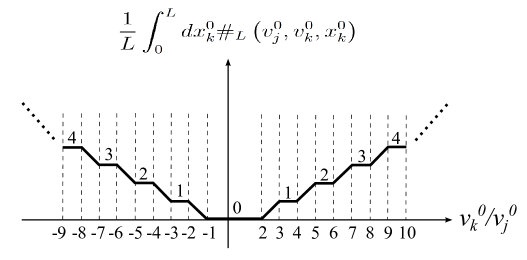
Figure 5: $\frac{1}{L}\int_{0}^{L}dx_{k}^{0}\#_{L}\left(v_{j}^{0},v_{k}^{0},x_{k}^{0}\right)$ as a function of $v_{k}^{0}/v_{j}^{0}$. The line segments connecting two adjacent flat parts are straight lines with slopes being $\pm 1$.

Let’s see what do Fig. 5 and Eq.17 mean. To have a backward collision with the main particle, a background particle needs to fly fast enough to catch up with the main particle, which can be seen from $\frac{1}{L}\int_{0}^{L}dx_{k}^{0}\#_{L}\left(v_{j}^{0},v_{k}^{0},x_{k}^{0}\right)=0$ for $-1<\left(v_{k}^{0}/v_{j}^{0}\right)<2$ in Fig. 5. Comparing the initial situation at $t=0$ and the final situation at $t=T_{j}^{0}/2$, all background particles change from sitting at the right side of the main particle to its left side. Therefore, the number of forward collisions is larger than the number of backward collisions by one, as shown in Eq.17.

Another viewpoint for the number of collisions is considering the condition of neighbor particles surrounding the main particle to collide with the main particle. The admissible velocities of neighbor particles causing forward collisions and backward collisions are $\left(-\infty,v_{j}^{0}\right)$ and $\left(v_{j}^{0},\infty\right)$, respectively, and hence forward collisions are more than backward collisions.

For a given $\left(x_{k}^{0},v_{k}^{0}\right)$, the corresponding $v_{k}$ can be found, with the help of $x-t$ diagram. Substituting the position distribution (homogeneous), the velocity distribution (Maxwellian), $\#_{R}$, $\#_{L}$ and $v_{k}$ into Eq.14, we have

$$\frac{1}{2}\Delta T_{j}^{0}=-r_{0}\frac{N}{v_{j}^{0}}+\frac{N}{2}\frac{1}{\sqrt{a\pi}\left(v_{j}^{0}\right)^{2}}\int_{0}^{\infty}dv_{k}^{0}\left[e^{-\frac{\left(v_{k}^{0}-v_{j}^{0}\right)^{2}}{a}}-e^{-\frac{\left(v_{k}^{0}+v_{j}^{0}\right)^{2}}{a}}\right]\left(v_{k}^{0}\right)^{2}\Delta t_{interaction}\left(0,v_{k}^{0}\right).$$ (18)

3.2.2 Correction of flying time period

Obtain $\Delta t_{interaction}\left(0,v_{k}^{0}\right)$ by Eq.12 for square well potential and then put it into Eq.18. Expand with $\frac{\epsilon}{k_{B}T}$ to $\mathcal{O}\left(\frac{\epsilon}{k_{B}T}\right)$. We have

$$\frac{1}{2}\Delta T_{j}^{0}=-\frac{Nd_{1}}{v_{j}^{0}}-\frac{N\left(d_{2}-d_{1}\right)\sqrt{a\pi}}{\left(v_{j}^{0}\right)^{2}}e^{-\frac{\left(v_{j}^{0}\right)^{2}}{a}}\mathrm{erfi}(\frac{v_{j}^{0}}{\sqrt{a}})\frac{\epsilon}{k_{B}T}.$$ (19)

This is the flying time period correction for square well potential.

Let’s try to figure out the physics behind Eq.19. The effect of hard core is decreasing the space that a particle can move, and the corresponding flying time correction is $\frac{1}{2}\Delta T_{j}^{0}=-Nd_{1}/v_{j}^{0}$. The second term is the effect of the attraction potential. It is always negative, which means that all particles are sped up. But why? The physics can be analyzed by average velocity $v_{j}\mid_{average}=\frac{2\left(L-Nd_{1}\right)}{T_{j}^{0}+\Delta T_{j}^{0}}$. By Eq.19, we get

$$\frac{u_{j}\mid_{average}-u_{j}^{0}}{\rho\left(d_{2}-d_{1}\right)\frac{\epsilon}{k_{B}T}}=\sqrt{\pi}e^{-\left(u_{j}^{0}\right)^{2}}\mathrm{erfi}(u_{j}^{0}).$$ (20)

(Recall that $u\equiv v/\sqrt{a}$.) The result is shown in Fig. 6.

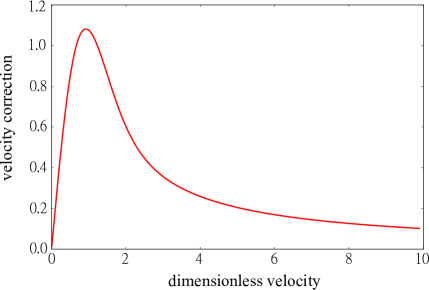
Figure 6: Correction of average velocity due to particle-particle attraction for square well potential. The x-axis is $u_{j}^{0}$ and the y-axis is $\frac{u_{j}\mid_{average}-u_{j}^{0}}{\rho\left(d_{2}-d_{1}\right)\frac{\epsilon}{k_{B}T}}$ given by Eq.20.

In Fig. 6, we have three features: $u_{j}\mid_{average}-u_{j}^{0}>0$, an increasing trend and a decreasing trend. In the following, we analyze the three features by number of collisions and effect of each collision.

For particle-particle attraction, when the main particle has a forward collision, its velocity is increased; when the main particle has a backward collision, its velocity is decreased. Since forward collisions are more than backward collisions, a particle is sped up when particle-particle attraction is turned on.

By Eq.17 and Fig. 5, the number of collisions provided by a background particle (with position distribution having been averaged by $\frac{1}{L}\int_{0}^{L}dx_{k}^{0}$) can be written as

$$1\ \mathrm{forward\ collision}+n\ \left(\mathrm{forward\ collision},\mathrm{backward\ collision}\right)\ \mathrm{pair},$$ (21)

where $n=\frac{1}{L}\int_{0}^{L}dx_{k}^{0}\#_{L}\left(v_{j}^{0},v_{k}^{0},x_{k}^{0}\right)$. For a background particle, the effect of a $(\mathrm{forward\ collision},$ $\mathrm{backward\ collision})$ pair is decreasing the velocity of the main particle, since the effect of particle-particle interaction is significant when the relative velocity is small. The feature that nonvanishing $n$ decreases as $v_{j}^{0}$ increases leads to the increasing trend in Fig. 6.

Velocity domain of background particles having significant contributions is a small neighborhood around $v_{j}^{0}$. When $v_{j}^{0}$ increases, the velocity of this small neighborhood also increases, and hence the population in this domain decreases, due to the exponential decay of Maxwell’s velocity distribution. This is the reason for the decreasing trend.

In the traditional picture of an interacting gas, particle-particle interaction disappears for the bulk part under mean field approximation [23]. With our mechanical approach, now we know that such handwaving picture is actually incorrect. Background particles are uniform, but the effect is not zero, since the main particle flies to a certain direction and thus breaks forward-backward symmetry. (The admissible velocities of neighbor particles causing forward collisions and backward collisions are $\left(-\infty,v_{j}^{0}\right)$ and $\left(v_{j}^{0},\infty\right)$, respectively.) The effect of forward collisions and the effect of backward collisions don’t cancel out. A particle is sped up when particle-particle attraction is turned on.

3.3 Temperature modification

Now let’s deal with the thermodynamic issue of “What is the real temperature of the system?” In Section 3.2, we see that particles fly faster when particle-particle attraction is turned on. Consequently, the temperature $T_{real}$ of the box of interacting gas is greater than it was ($T$) before the interaction is turned on. What this means is that, one really should start with an ideal gas with a suitably chosen lower temperature to perform the perturbation calculation, so that in the end the combined effect of the added interaction will raise the temperature of the system to the desired temperature. So what is the relation between $T_{real}$ and $T$?

The idea is, for average kinetic energy $\left\langle K.E.\right\rangle$, we should get $N\left\langle K.E.\right\rangle=\frac{N}{2}k_{B}T_{real}$. That is, the real temperature should be introduced by

$$\sum_{j}\frac{1}{2}m\left(v_{j}\mid_{average}\right)^{2}=\frac{N}{2}k_{B}T_{real}.$$ (22)

Putting $v_{j}\mid_{average}=\frac{2\left(L-Nd_{1}\right)}{T_{j}^{0}+\Delta T_{j}^{0}}$ and $\sum_{j}\frac{1}{2}m\left(v_{j}^{0}\right)^{2}=\frac{N}{2}k_{B}T$ into Eq.22, we get

$$\frac{N}{2}k_{B}T_{real}=\frac{N}{2}k_{B}T\left(1-2\rho d_{1}\right)-\sum_{j}m\left(v_{j}^{0}\right)^{2}\frac{\Delta T_{j}^{0}}{T_{j}^{0}}.$$ (23)

Eq.23 is the relation between $T_{real}$ and $T$. Putting Eq.23 into Eq.8, the equation of state is modified to

$$F=\rho k_{B}T_{real}+2\rho^{2}\left(k_{B}T_{real}\right)d_{1}+\sum_{j}\frac{2mv_{j}^{0}}{T_{j}^{0}}\frac{\Delta T_{j}^{0}}{T_{j}^{0}}+\sum_{j}\frac{2m\Delta v_{j}^{0}}{T_{j}^{0}}.$$ (24)

Actually, the idea of temperature modification can also be seen by considering the total energy of the box of gas. In our current formulation, turning on the interaction does not change the total energy of the system. Thus, on the one hand, this total energy should be equal to the total kinetic energy of the unperturbed ideal gas, which implies

$$\mathrm{total}\ \mathrm{energy}=\sum_{j}\frac{1}{2}m\left(v_{j}^{0}\right)^{2}=\frac{N}{2}k_{B}T.$$ (25)

On the other hand, this total energy becomes the summation of the average kinetic energy and average potential energy of each particle, which reads

$$\mathrm{total}\ \mathrm{energy}=\frac{N}{2}k_{B}T_{real}+N\left\langle U\right\rangle.$$ (26)

Comparing the above two expressions for the same total energy, we have

$$k_{B}T_{real}=k_{B}T-2\left\langle U\right\rangle.$$ (27)

Therefore, $T_{real}>T$ when particle-particle attraction is turned on, just as claimed before.

Note that we can see that traditional interpretation of the van der Waals equation adopting mean field approximation is incorrect simply by $\sum_{j}\frac{1}{2}m\left(v_{j}^{0}\right)^{2}=\sum_{j}\frac{1}{2}m\left(v_{j}\mid_{average}\right)^{2}+N\left\langle U\right\rangle$, without doing detailed calculations. When particle-particle attraction is turned on, potential energy is negative and hence particles move faster.

3.4 Momentum transferred (physics on the boundary)

Collision velocity of the main particle is determined by its state hitting the right wall. How to find out the state of the main particle at $t=T_{j}^{0}/2$? The idea is, the main particle experiences lots of collisions during its entire trip, and the last one determines its behavior at $t=T_{j}^{0}/2$. If the position of the last collision of the main particle is close to the right wall such that particle-wall collision is simultaneously happening when two particles are interacting, nonvanishing $\Delta v_{j}^{0}$ appears. That is, nonvanishing $\Delta v_{j}^{0}$ appears once the wall comes into play during the interaction and thus interrupts the otherwise “normal” interaction.

In order to deal with the effect of $\Delta v_{j}^{0}$, we collect the cases having nonvanishing $\Delta v_{j}^{0}$. The effect of $\Delta v_{j}^{0}$ can be decomposed into two parts. The first part is about the probability of a given situation of the last collision (Section 3.4.1). The second part is about the effect associated with a given situation of the last collision (Section 3.4.2). The total effect is the product of the two parts (Section 3.4.3).

3.4.1 Probability of the last collision

The setting of the start of the last collision is that the main particle is at $L-d_{3}$ and the background particle that causes the last collision hits the main particle with $v_{k}^{0}$. The probability of such scenario is studied in Appendix A, and is given by

$$N\left(\left|1-\frac{v_{k}^{0}}{v_{j}^{0}}\right|\frac{\Delta d_{3}}{L}\right)\left(f\left(v_{k}^{0}\right)\Delta v_{k}^{0}\right)\mathrm{exp}\left\{-\frac{1}{2}\left[1+\mathrm{erf}\left(\frac{v_{j}^{0}}{\sqrt{a}}\right)+\frac{\sqrt{a}}{\sqrt{\pi}v_{j}^{0}}e^{-\frac{\left(v_{j}^{0}\right)^{2}}{a}}\right]\rho d_{3}\right\}.$$ (28)

3.4.2 Situation around the wall

Let’s consider non-trivial situations (nonvanishing $\Delta v_{j}^{0}$) of the last collision of the main particle around the wall. For square well potential, the relation between $v_{in}$ and $v_{out}$ ($v_{in}$ and $v_{out}$ are the speeds inside and outside the potential well, respectively, defined in the center-of-mass frame of the two interacting particles.) is

$$v_{in}=\sqrt{\left(v_{out}\right)^{2}+\frac{\epsilon}{m}}.$$ (29)

Particle-particle interaction is easy to analyze in the center-of-mass frame. To investigate the role played by the wall, lab frame is a better choice. Therefore, we will switch between center-of-mass frame and lab frame. Note that collision velocity is defined in the lab frame. In the following analysis, we separate the situations of the last collision into forward collision part and backward collision part.

Forward collision part

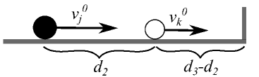
Figure 7: The initial state of the last collision being a forward collision.

The situation for the beginning of forward collision is shown in Fig. 7. $v_{k}^{0}$ is not arbitrary. First, the occurrence of forward collision implies $v_{k}^{0}<v_{j}^{0}$. Second, if $v_{CM}=\left(v_{j}^{0}+v_{k}^{0}\right)/2$ is not positive, the two particles don’t hit the wall until their interaction is over. Combining the two considerations, the condition for $v_{k}^{0}$ is

$$-v_{j}^{0}<v_{k}^{0}<v_{j}^{0}.$$ (30)

For the main particle to hit the wall when it is still in the potential well, $d_{3}$ should be short enough. The range of $d_{3}$ and the collision velocity is presented in Appendix B.

We put the range of $d_{3}$ and the collision velocity in appendix because it is the range of $v_{k}^{0}$ that plays the truly significant role for the feature of physics on the boundary. The role of the range of $v_{k}^{0}$ will be clear in Section 3.4.3 and Section 4.1.

Backward collision part

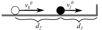
Figure 8: The initial state of the last collision being a backward collision.

The situation for the beginning of backward collision is shown in Fig. 8. The occurrence of backward collision implies

$$v_{k}^{0}>v_{j}^{0}.$$ (31)

The range of $d_{3}$ and the collision velocity is presented in Appendix C.

3.4.3 Correction of collision velocity

Having considered all the factors, we are now in a position to actually calculate the combined result for $\Delta v_{j}^{0}$. The total effect is the product of “probability of a given situation of the last collision” (Section 3.4.1, Appendix A) and “effect associated with a given situation of the last collision” (Section 3.4.2, Appendix B and Appendix C). The derivation is in Appendix D, E, and F. Finally, we get

	in the bulk	on the boundary
forward collision	$-\infty\sim v_{j}^{0}$	$-v_{j}^{0}\sim v_{j}^{0}$
backward collision	$v_{j}^{0}\sim\infty$	$v_{j}^{0}\sim\infty$

Table 1: Velocity domains of neighbor particles (surrounding the main particle) that cause forward and backward collisions.

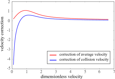
Figure 9: Correction of average velocity and correction of collision velocity for square well potential. The x-axis is $u_{j}^{0}$. The upper curve is the correction of average velocity given by $\frac{u_{j}\mid_{average}-u_{j}^{0}}{\rho\left(d_{2}-d_{1}\right)\frac{\epsilon}{k_{B}T}}$ in Eq.20. The lower curve is the correction of collision velocity given by $\frac{\left(u_{j}^{0}+\Delta u_{j}^{0}\right)-u_{j}^{0}}{\rho\left(d_{2}-d_{1}\right)\frac{\epsilon}{k_{B}T}}$ in Eq.32.

$$\frac{\Delta u_{j}^{0}}{\rho\left(d_{2}-d_{1}\right)\frac{\epsilon}{k_{B}T}}=\frac{1}{2\sqrt{\pi}u_{j}^{0}}\left(\int_{-u_{j}^{0}}^{\infty}du_{k}^{0}e^{-\left(u_{k}^{0}\right)^{2}}\frac{u_{j}^{0}+u_{k}^{0}}{u_{j}^{0}-u_{k}^{0}}+\int_{u_{j}^{0}}^{\infty}du_{k}^{0}e^{-\left(u_{k}^{0}\right)^{2}}\frac{u_{j}^{0}-u_{k}^{0}}{u_{j}^{0}+u_{k}^{0}}\right).$$ (32)

The result is shown in Fig. 9.

The profile of $\Delta u_{j}^{0}$ in Fig. 9 can be understood as we decompose the profile into two main trends, an increasing trend and a decreasing trend. From Table 1, for physics on the boundary, as $u_{j}^{0}$ increases, number of relevant forward collisions increases and number of relevant backward collisions decreases. So $\Delta u_{j}^{0}$ increases as $u_{j}^{0}$ increases. As for the decreasing trend, the physics is the same as the decreasing trend for $\left(u_{j}\mid_{average}-u_{j}^{0}\right)$. Analysis here is like what we do for the profile of $\left(u_{j}\mid_{average}-u_{j}^{0}\right)$ in Fig. 6. The underlying physics are both collision number and exponential decay suppression. This is why $\Delta u_{j}^{0}$ and $\left(u_{j}\mid_{average}-u_{j}^{0}\right)$ have similar profiles in Fig. 9.

We can see that average velocity is always larger than collision velocity. We will come back to the physical meaning of this feature later when studying generic particle-particle interaction.

3.4.4 Correction of momentum transferred in equation of state

It’s time to complete the last mile to a full description of the correction of momentum transferred in equation of state. Plugging Eq.32 into $\sum_{j}\left(2m\Delta v_{j}^{0}/T_{j}^{0}\right)$, we get

$$\sum_{j}\frac{2m\Delta v_{j}^{0}}{T_{j}^{0}}=0.$$ (33)

In order to obtain $\sum_{j}\left(2m\Delta v_{j}^{0}/T_{j}^{0}\right)$, we went through all the calculations from Section 3.4.1 to Section 3.4.3 and all the appendices, and yet the final result is just zero! What’s going on? For obtaining such simple result after a long calculation, we had better give a story. So here is the story.

Note that what we have is $\sum_{j}\left(2m\Delta v_{j}^{0}/T_{j}^{0}\right)=0$ but not $\left(2m\Delta v_{j}^{0}/T_{j}^{0}\right)=0$. A summation giving zero often relates to conservation law. This is the first hint for the physics behind Eq.33.

In our construction, $v_{j}^{0}+\Delta v_{j}^{0}$ is the collision velocity that a particle hits the wall. A different viewpoint is that the wall is a momentum provider, since it provides some momentum to the box of gas every time a particle hits it. Let’s check the total positive momentum of the system. For a box of $N$ particles, in order to have an idea of total positive momentum that is separate from total negative momentum, we take a snapshot for the box of gas and pull apart all particle pairs, and then define total positive momentum and total negative momentum by these $N$ decoupled particles.

When the box of gas is at thermal equilibrium, it is a steady state, and hence the total positive momentum is time-independent. After the system evolves for $\Delta t$, what is the total positive momentum now? For a particle with $v_{j}^{0}>0$ having initial position in $\left(L-v_{j}^{0}\Delta t,L\right)$, its velocity will be negative at $t=\Delta t$. When counting the total positive momentum at $t=\Delta t$, such particle has no contribution. Such particles have the population of $\left(v_{j}^{0}\Delta t\right)/L=\Delta t/\frac{1}{2}T_{j}^{0}$. When counting the total positive momentum at $t=\Delta t$, momentum loss due to the effect that a particle can change its direction is given by

$$\mathrm{momentum\ loss}=\sum_{j}\frac{\Delta t}{\frac{1}{2}T_{j}^{0}}\left(-mv_{j}^{0}\right).$$ (34)

On the other hand, we also have momentum gain due to the reflection provided by the left wall. For each collision, the left wall provides a momentum of $m\left(v_{j}^{0}+\Delta v_{j}^{0}\right)$ to the total positive momentum of the system. Momentum gain provided by the left wall during $\Delta t$ is

$$\mathrm{momentum\ gain}=\sum_{j}\frac{\Delta t}{\frac{1}{2}T_{j}^{0}}\left(m\left(v_{j}^{0}+\Delta v_{j}^{0}\right)\right).$$ (35)

Since the total positive momentum of the system is time-independent, by Eq.34 and Eq.35, we have

$$\sum_{j}\frac{2m\Delta v_{j}^{0}}{T_{j}^{0}}=0.$$ (36)

By requiring the system to be a steady state, we can get $\sum_{j}\left(2m\Delta v_{j}^{0}/T_{j}^{0}\right)=0$. However, it cannot tell us the $v_{j}^{0}-\mathrm{dependence}$ of $\Delta v_{j}^{0}$, since we have summed over all $v_{j}^{0}$ and thus lost such information. Such information can be figured out only if we study individual $\Delta v_{j}^{0}$. This is one merit of the mechanical model for calculating $\Delta v_{j}^{0}$ (Eq.32 and Fig. 9).

3.5 Equation of state

Now we are ready to write down the equation of state for a one-dimensional gas with square well potential. Putting Eq.19 and Eq.36 into Eq.24 and keeping the physics to the lowest order of particle-particle interaction, we have

$$F=\rho k_{B}T_{real}+\rho^{2}\left(k_{B}T_{real}\right)d_{1}-\rho^{2}\left(d_{2}-d_{1}\right)\epsilon.$$ (37)

This is the equation of state for square well potential in our mechanical approach, and it gives the same answer as statistical mechanics (Eq.9).

The physical meaning behind Eq.37 is a little subtle. Putting Eq.19 and Eq.36 into Eq.8, we have the equation of state of form

$$F=\rho k_{B}T+\rho^{2}\left(k_{B}T\right)d_{1}+\rho^{2}\left(d_{2}-d_{1}\right)\epsilon.$$ (38)

As a limiting case, let us neglect the hard core and consider only the effect of the particle-particle attraction. By Eq.37 and Eq.38, we have

$$\rho k_{B}T<F<\rho k_{B}T_{real}.$$ (39)

Thus, to the naive question of “When particle-particle attraction is turned on, is the force increased or decreased?” the answer is that the force is actually increased. But one should follow by the immediate qualifier that, “the temperature of the system is also increased.” However, if we are comparing the force exerted by an ideal gas and that by a van der Waals gas at the same temperature, but with the particle size effect ignored, then the van der Waals gas necessarily exerts a smaller force.

4 One-dimensional interacting gas with generic particle-particle interaction

With the lessons learnt from one-dimensional interacting gas with square well potential, we can generalize the mechanical model to generic one-dimensional interacting gas. By generic particle-particle interaction, we mean the potential is consisted of a hard core and an interaction tail with finite range $r_{0}$. In the following, we study attraction tail and then repulsion tail.

4.1 Particle-particle attraction

Obtain $\Delta t_{interaction}\left(0,v_{k}^{0}\right)$ by Eq.12 and then put it into Eq.18. Expand with $\frac{U(r)}{k_{B}T}$ to $\mathcal{O}\left(\frac{U(r)}{k_{B}T}\right)$. We have

$$\frac{1}{2}\Delta T_{j}^{0}=-\frac{Nd_{1}}{v_{j}^{0}}-\frac{N\sqrt{a\pi}}{\left(v_{j}^{0}\right)^{2}}e^{-\frac{\left(v_{j}^{0}\right)^{2}}{a}}\mathrm{erfi}(\frac{v_{j}^{0}}{\sqrt{a}})\left(\int_{d_{1}}^{r_{0}}dr\left[-\frac{U(r)}{k_{B}T}\right]\right).$$ (40)

Eq.40 is just Eq.19, with $\left(d_{2}-d_{1}\right)\frac{\epsilon}{k_{B}T}$ replaced by $\left(\int_{d_{1}}^{r_{0}}dr\left[-\frac{U(r)}{k_{B}T}\right]\right)$. Therefore, the physics is all the same. For generic particle-particle interaction being attractive, $U(r)$ is negative and particles are sped up. Putting Eq.36 and Eq.40 into Eq.24, we obtain

$$F=\rho k_{B}T_{real}+\rho^{2}\left(k_{B}T_{real}\right)d_{1}-\rho^{2}\left(\int_{d_{1}}^{r_{0}}dr\left[-U(r)\right]\right).$$ (41)

This is exactly the equation of state derived using standard statistical mechanics, as we show in Eq.2.

The physics behind Eq.41 is the same as what we present in Section 3. Now we want to analyze the physics from another viewpoint basing on the idea of average velocity. Instead of separating $\Delta T_{j}^{0}$ from $T_{j}=T_{j}^{0}+\Delta T_{j}^{0}$ (what we do from Eq.7 to Eq.8), we can regard $T_{j}$ as an entire entity and then work with the idea of average velocity ($v_{j}\mid_{average}=2\left(L-Nd_{1}\right)/T_{j}$) directly but not the free particle velocity. In such approach, “physics in the bulk” is simply embedded in the idea of average velocity. By our very construction, the only effect to be considered is what happens when a particle hits the wall.

Rewrite the equation of state with average velocity and collision velocity. Start from Eq.7 and keep the physics to the first order in the particle-particle interaction, and we have

$$F=\rho k_{B}T_{real}+\rho^{2}\left(k_{B}T_{real}\right)d_{1}+\frac{m}{L}\sum_{j}\left(v_{j}\mid_{average}\right)\left(\left(v_{j}^{0}+\Delta v_{j}^{0}\right)-v_{j}\mid_{average}\right).$$ (42)

Compared with Eq.41, for particle-particle interaction being attractive, the third term in Eq.42 should be negative. The reason hides in Table 1. From Table 1, we can see that, on the average, a particle experiences more forward collisions from its neighbors when it is in the bulk than it is on the boundary. Therefore, we have

$$\left(v_{j}^{0}+\Delta v_{j}^{0}\right)-v_{j}\mid_{average}<0.$$ (43)

The feature that $\left(v_{j}^{0}+\Delta v_{j}^{0}\right)-v_{j}\mid_{average}<0$ can be seen in Fig. 9. So now we understand that it is caused by the fact that the two kinds of velocities have different numbers of forward collisions.

In a naive description trying to explain the form of the van der Waals equation [23], one is tempted to claim that a particle hitting the wall is slowed down due to the attraction of other gas particles from the back, and hence the force felt by the wall is decreased. Put differently, this seemingly plausible theory claims that the velocity hitting the wall (collision velocity) is smaller than the velocity in the bulk (average velocity), which also holds true in our detailed mechanical approach.

However, we must quickly point out that, as particle-particle attraction is turned on, physics in the bulk is non-trivial and particles in the box do fly faster. The reason that we don’t need to consider average velocity correction in the conventional description of the van der Waals equation is not because forward collisions and backward collisions cancel out exactly (they don’t), but lies in the fact that they are all lumped into the idea of $v_{j}\mid_{average}$. Now it is clear that traditional picture of the van der Waals equation actually uses $v_{j}\mid_{average}$ but not $v_{j}^{0}$ in the argument. For physics in the bulk, it just takes the net result ($v_{j}\mid_{average}$) and then bypasses all the issues related to “what happens when a particle flies in the middle of the box,” including temperature modification. It is in this sense that traditional picture makes sense.

4.2 Particle-particle repulsion

For particle-particle repulsion, we just reverse the physics of attraction tail. However, one feature does stand out that is characteristic to particle-particle repulsion alone. When the relative velocity of two interacting particles is small, they don’t have enough kinetic energy (in center-of-mass frame) to overcome the potential barrier and reach $r=d_{1}$. Nevertheless, the population of such particle pairs is quite small since particle-particle interaction is weak by our construction, and hence such effect is negligible in equation of state.

Another issue related to particle-particle repulsion is soft core. An example of soft core is Lennard-Jones potential, which has a $r^{-12}$ repulsive term. Can we attack soft core in our mechanical approach? The answer is a sadly no. Soft core aims to stop two colliding particles, and this goal needs strong particle-particle interaction that cannot be treated as a perturbation. Nonperturbative approach is needed for studying soft core.

5 Conclusion

In this work, we have taken a mechanical approach to a one-dimensional interacting gas with particle-particle interaction made up of a hard core and an interaction tail. Perturbations around ideal gas are considered and the physics is computed correct up to $\mathcal{O}\left(\frac{U}{k_{B}T}\right)$. Equation of state given by our mechanical approach matches the result given by statistical mechanics. Assumptions and conditions we put in by hand include (1) the homogeneity assumption on the spatial distribution, (2) velocity distribution being Maxwellian, (3) the system being in steady state, (4) short range and weak interparticular interaction, (5) low density, and (6) high temperature, all of which are common assumed in traditional statistical mechanics.

5.1 Summary

Besides having been able to reproduce the equation of state, we do obtain some physics insight that traditional statistical mechanics doesn’t readily tell us. In the following, we list six points for the effects of particle-particle attraction. Almost all the physics in the mechanical model is hidden in Fig. 9 and Table 1.

(1) Due to the fact that the number of forward collisions is larger than the number of backward collisions, on the average, all particles move faster in the presence of particle-particle attraction.

(2) Since particles move faster as particle-particle attraction is turned on, the temperature of the system increases. Another point of view without concerning mechanics is considering total energy of the system.

(3) For a slow particle, $\Delta v_{j}^{0}<0$. For a fast particle, $\Delta v_{j}^{0}>0$. The increase and decrease of collision velocity necessarily cancel out due to our very assumption that the system is a steady state.

(4) Average velocity correction and collision velocity correction have similar trends since the physics are similar. When the main particle moves fast, the effect of forward collisions dominates and it leads to the increasing trend. Suppression of the effect of particle-particle interaction by exponential decay in Maxwell’s velocity distribution is responsible for the decreasing trend.

(5) Compared with collision velocity, average velocity has more forward collisions, and hence average velocity is bigger than collision velocity.

(6) Compared with $\rho k_{B}T$, the force is increased. But compared with $\rho k_{B}T_{real}$, the force is decreased.

5.2 Meaning and implication

Unlike most researches studying N-body systems in the framework of statistical mechanics or kinetic theory, we take a mechanical approach to a one-dimensional weakly interacting gas in thermal equilibrium. With the help from a detailed analysis of how gas particles interact, we have successfully gained some more interesting physics that the traditional approach doesn’t readily tell us. Our work is an example demonstrating the possibility to study weakly interacting N-body systems from a mechanical viewpoint working with particle trajectory.

Though the derivation here is focused on the equation of state, the spirit of this mechanical model is investigating the physics of particle-particle interaction and trying to have deeper understanding. With this mechanical model, we obtain some understanding for issues other than the equation of state.

How do we construct such mechanical model? There are three elements: (1) a mechanical picture for unperturbed part (free particle model), (2) plausible assumptions concerning things such as the velocity distribution and homogeneity of the system that we put in by hand, and (3) assumed form of (weak) particle-particle interaction. Adding the effect of particle-particle interaction on free particle model, we capture some interesting physics. The essence of such mechanical model lies in the fact that the effect of particle-particle interaction is weak ($\mathcal{O}\left(\rho r_{0}\right)<\mathcal{O}\left(1\right)$ and $\mathcal{O}\left(\frac{U}{k_{B}T}\right)<\mathcal{O}\left(1\right)$), and so in some sense we can have the notion of particle trajectory and focus on two-body interaction. For a system different from one-dimensional interacting gas (some colloidal systems or granular systems, for example), if we can figure out its free particle model and then put in particle-particle interaction, maybe we can have some interesting physics. We think it is possible to extend the idea to other systems that are usually studied in a statistical mechanics or kinetic theory point of view.

Statistical mechanics works with partition function. Traditional kinetic theory adopting Boltzmann equation considers a particle interacting with its neighbor particles. Our mechanical approach works with a more detailed analysis of the particle trajectory, the number of collisions and the effect of each collision. The merit of this mechanical approach is that it does provide us with more physics insight about how the individual effect affects the final answer.

Appendix A: Probability of the last collision

In this appendix, we calculate the probability of the last collision. To find the probability of such situation, we put in the background particles one by one. The probability of the background particle that causes the last collision is given by

$$\left(\left|1-\frac{v_{k}^{0}}{v_{j}^{0}}\right|\frac{\Delta d_{3}}{L}\right)\left(f\left(v_{k}^{0}\right)\Delta v_{k}^{0}\right).$$ (44)

For the remaining $N-2$ background particles, they should be put in the box in the manner that they cannot touch the main particle after the main particle has its last collision with the first background particle. The position of one of the remaining $N-2$ background particles with free particle velocity $v_{l}^{0}$ at $t=\left(L-d_{3}\right)/v_{j}^{0}$ is denoted as $\widetilde{x_{l}}$. The requirement for $\widetilde{x_{l}}$ is

$$0<\widetilde{x_{l}}<L-d_{3},$$ (45)

and the admissible velocity is

$$-\frac{L+\widetilde{x_{l}}}{d_{3}}v_{j}^{0}<v_{l}^{0}<\frac{L-\widetilde{x_{l}}}{d_{3}}v_{j}^{0}.$$ (46)

The probability of a single background particle in the admissible zone is thus given by

$$\int_{0}^{L-d_{3}}\frac{d\widetilde{x_{l}}}{L}\int_{-\frac{L+\widetilde{x_{l}}}{d_{3}}v_{j}^{0}}^{\frac{L-\widetilde{x_{l}}}{d_{3}}v_{j}^{0}}dv_{l}^{0}\frac{1}{\sqrt{a\pi}}e^{-\frac{\left(v_{l}^{0}\right)^{2}}{a}}.$$ (47)

When thermodynamic limit is considered, we have

$$\mathrm{probability\ }\mathrm{of}\ (N-2)\ \mathrm{background}\ \mathrm{particles}=\mathrm{exp}\left\{-\frac{1}{2}\left[1+\mathrm{erf}\left(\frac{v_{j}^{0}}{\sqrt{a}}\right)+\frac{\sqrt{a}}{\sqrt{\pi}v_{j}^{0}}e^{-\frac{\left(v_{j}^{0}\right)^{2}}{a}}\right]\rho d_{3}\right\}.$$ (48)

The complete probability of the last collision is the product of Eq.44 and Eq.48 and the permutation factor $N$, and is given by

$$N\left(\left|1-\frac{v_{k}^{0}}{v_{j}^{0}}\right|\frac{\Delta d_{3}}{L}\right)\left(f\left(v_{k}^{0}\right)\Delta v_{k}^{0}\right)\mathrm{exp}\left\{-\frac{1}{2}\left[1+\mathrm{erf}\left(\frac{v_{j}^{0}}{\sqrt{a}}\right)+\frac{\sqrt{a}}{\sqrt{\pi}v_{j}^{0}}e^{-\frac{\left(v_{j}^{0}\right)^{2}}{a}}\right]\rho d_{3}\right\}.$$ (49)

Appendix B: Physics on the boundary for forward collision

In this appendix, we study the range of $d_{3}$ and the collision velocity for forward collision. By Eq.10 and Eq.29, the condition for $d_{3}$ is

$$d_{3}<d_{2}+\left(d_{2}-d_{1}\right)\frac{\frac{v_{j}^{0}+v_{k}^{0}}{2}}{\sqrt{\left(\frac{v_{j}^{0}-v_{k}^{0}}{2}\right)^{2}+\frac{\epsilon}{m}}}.$$ (50)

If the main particle hits the wall when it is in the potential well, by Eq.29, the collision velocity is

$$v_{j}^{0}+\Delta v_{j}^{0}=\frac{v_{j}^{0}+v_{k}^{0}}{2}+\sqrt{\left(\frac{v_{j}^{0}-v_{k}^{0}}{2}\right)^{2}+\frac{\epsilon}{m}}.$$ (51)

By Eq.30, Eq.50 and Eq.51, the nonvanishing $\Delta v_{j}^{0}$ in forward collision part is summarized in Fig. 10, with

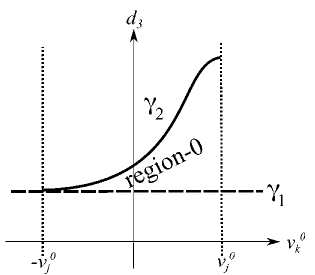
Figure 10: Nonvanishing $\Delta v_{j}^{0}$ in forward collision part. Nonvanishing $\Delta v_{j}^{0}$ appears in region-0. Detailed information is given by Eq.52 and Eq.53.

$$\gamma_{1} : d_{3}=d_{2},$$

$$\gamma_{2} : d_{3}=d_{2}+\left(d_{2}-d_{1}\right)\frac{\frac{v_{j}^{0}+v_{k}^{0}}{2}}{\sqrt{\left(\frac{v_{j}^{0}-v_{k}^{0}}{2}\right)^{2}+\frac{\epsilon}{m}}},$$ (52)

$$\Delta v_{j}^{0}\mid_{region-0}=\frac{-v_{j}^{0}+v_{k}^{0}}{2}+\sqrt{\left(\frac{v_{j}^{0}-v_{k}^{0}}{2}\right)^{2}+\frac{\epsilon}{m}}.$$ (53)

Appendix C: Physics on the boundary for backward collision

In this appendix, we study the range of $d_{3}$ and the collision velocity for backward collision. By Eq.10 and Eq.29, the condition for $d_{3}$ is

$$\left(d_{2}+d_{3}\right)<d_{2}+\left(d_{2}-d_{1}\right)\frac{\frac{v_{j}^{0}+v_{k}^{0}}{2}}{\sqrt{\left(\frac{v_{j}^{0}-v_{k}^{0}}{2}\right)^{2}+\frac{\epsilon}{m}}}.$$ (54)

Eq.31 and Eq.54 are necessary conditions to have nonvanishing $\Delta v_{j}^{0}$. Under the two necessary conditions, the situations can be classified as three classes (Class 1, Class 2 and Class 3) by different forms of collision velocities.

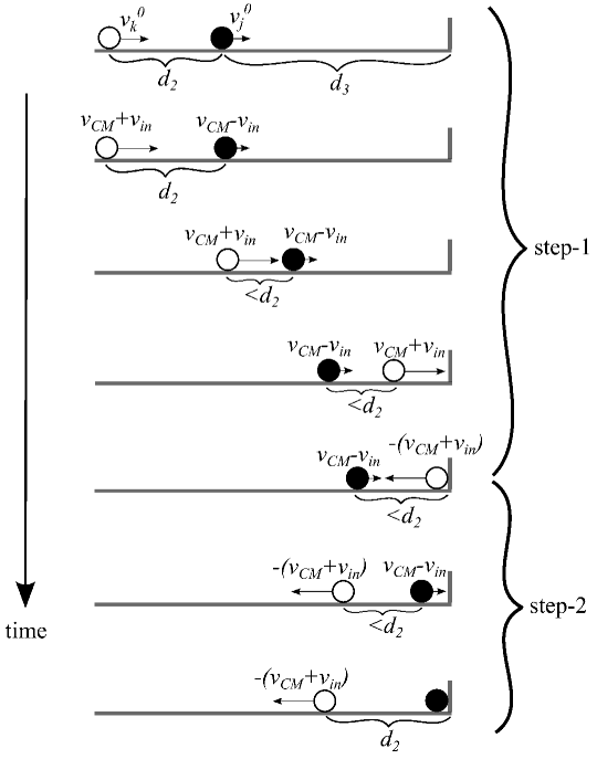
Figure 11: Critical situation that separates the three classes (Class 1, Class 2 and Class 3). The figure shows the motion of the main particle and the first background particle in the lab frame. Step-1 starts with the beginning of backward collision and ends with the event that the first background particle hits the wall. Step-2 starts with the end of step-1 and ends with the moment that the two particles are going to decouple. The value of $d_{3}$ in this critical situation is denoted as $d_{3}\mid_{critical}$.

The critical situation separating the three classes is shown in Fig. 11, with $d_{3}\mid_{critical}$ given by

$$d_{3}\mid_{critical}=\left(d_{2}-d_{1}\right)\left(\frac{\frac{v_{j}^{0}+v_{k}^{0}}{2}}{\sqrt{\left(\frac{v_{j}^{0}-v_{k}^{0}}{2}\right)^{2}+\frac{\epsilon}{m}}}-1\right).$$ (55)

Class 1:
In Class 1, $d_{3}<d_{3}\mid_{critical}$. In this class, the main particle hits the wall when it is in the potential well. The collision velocity is

$$v_{j}^{0}+\Delta v_{j}^{0}=\frac{v_{j}^{0}+v_{k}^{0}}{2}-\sqrt{\left(\frac{v_{j}^{0}-v_{k}^{0}}{2}\right)^{2}+\frac{\epsilon}{m}}.$$ (56)

Class 2:
In Class 2, $d_{3}>d_{3}\mid_{critical}$. In this class, the main particle hits the wall after it decouples with the first background particle and becomes a free particle again. However, the velocity of the main particle being a free particle is no longer $v_{j}^{0}$, since the wall comes into play and alters particle-particle interaction via particle-wall collision of the first background particle at the end of step-1. With the help of Eq.29, the new free particle velocity of the main particle, namely the collision velocity, is given by

$$v_{j}^{0}+\Delta v_{j}^{0}=\sqrt{\left(\frac{v_{j}^{0}+v_{k}^{0}}{2}\right)^{2}-\frac{\epsilon}{m}}-\sqrt{\left(\frac{v_{j}^{0}-v_{k}^{0}}{2}\right)^{2}+\frac{\epsilon}{m}}.$$ (57)

Class 3:
In Fig. 11, we actually already assume that the main particle always has a positive velocity. But this is not always guaranteed. If the main particle has a negative velocity, it cannot hit the wall, and the collision velocity in such case is zero. There are two situations when no collision happens between the main particle and the wall.

The first situation is that the velocity of the main particle is negative at the moment right after the collision starts. That is, $v_{CM}-v_{in}<0$. In this case, $v_{k}^{0}$ is given by

$$v_{k}^{0}<\frac{\frac{\epsilon}{m}}{v_{j}^{0}}.$$ (58)

The second situation is that the velocity of the main particle is negative after they decouple. That is, the new free particle velocity in Eq.57 is negative. In this case, $v_{k}^{0}$ is given by

$$\frac{\frac{\epsilon}{m}}{v_{j}^{0}}<v_{k}^{0}<\frac{2\frac{\epsilon}{m}}{v_{j}^{0}}.$$ (59)

In Class 1, the main particle hits the wall during its interaction with the first background particle. In Class 2, the main particle hits the wall when it becomes a free particle after it decouples with the first background particle. In Class 3, the main particle simply cannot hit the wall.

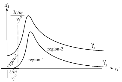
Figure 12: Nonvanishing $\Delta v_{j}^{0}$ in backward collision part. Region-1,2,3 corresponds to Class 1,2,3, respectively. In addition, region for $v_{k}^{0}<v_{j}^{0}$ is forbidden. Detailed information is given by Eq.60 and Eq.61.

The nonvanishing $\Delta v_{j}^{0}$ in backward collision part is summarized in Fig. 12, with

$$\gamma_{3} : d_{3}=\left(d_{2}-d_{1}\right)\left(\frac{\frac{v_{j}^{0}+v_{k}^{0}}{2}}{\sqrt{\left(\frac{v_{j}^{0}-v_{k}^{0}}{2}\right)^{2}+\frac{\epsilon}{m}}}-1\right),$$

$$\gamma_{4} : d_{3}=\left(d_{2}-d_{1}\right)\frac{\frac{v_{j}^{0}+v_{k}^{0}}{2}}{\sqrt{\left(\frac{v_{j}^{0}-v_{k}^{0}}{2}\right)^{2}+\frac{\epsilon}{m}}},$$ (60)

$$\mathrm{Class}\ 1 : \Delta v_{j}^{0}\mid_{region-1}=\frac{-v_{j}^{0}+v_{k}^{0}}{2}-\sqrt{\left(\frac{v_{j}^{0}-v_{k}^{0}}{2}\right)^{2}+\frac{\epsilon}{m}},$$

$$\mathrm{Class}\ 2 : \Delta v_{j}^{0}\mid_{region-2}=-v_{j}^{0}+\sqrt{\left(\frac{v_{j}^{0}+v_{k}^{0}}{2}\right)^{2}-\frac{\epsilon}{m}}-\sqrt{\left(\frac{v_{j}^{0}-v_{k}^{0}}{2}\right)^{2}+\frac{\epsilon}{m}},$$

$$\mathrm{Class}\ 3 : \Delta v_{j}^{0}\mid_{region-3}=-v_{j}^{0}.$$ (61)

Of course, we also have the condition of Eq.31, and hence the region that $v_{k}^{0}<v_{j}^{0}$ is forbidden. Therefore, Class 3 in backward collision part occurs only for small $u_{j}^{0}$ satisfying

$$u_{j}^{0}<\sqrt{\frac{\epsilon}{k_{B}T}}.$$ (62)

Appendix D: Total effect of the correction of collision velocity

In this appendix, we finally calculate the total effect of the correction of collision velocity. The task we are going to do is putting Eq.28 (probability), Eq.53 ($\Delta v_{j}^{0}$ for forward collision part) and Eq.61 ($\Delta v_{j}^{0}$ for backward collision part) together and then integrate over the four regions shown in Fig. 10 and Fig. 12. That is, we are going to deal with the integral

$$\Delta v_{j}^{0} = \rho\int d(d_{3})\int dv_{k}^{0}f\left(v_{k}^{0}\right)\left|1-\frac{v_{k}^{0}}{v_{j}^{0}}\right|\mathrm{exp}\left\{-\frac{1}{2}\left[1+\mathrm{erf}\left(\frac{v_{j}^{0}}{\sqrt{a}}\right)+\frac{\sqrt{a}}{\sqrt{\pi}v_{j}^{0}}e^{-\frac{\left(v_{j}^{0}\right)^{2}}{a}}\right]\rho d_{3}\right\}$$ (63)

$$\times\left(\Delta v_{j}^{0}\mid_{region-0}+\Delta v_{j}^{0}\mid_{region-1}+\Delta v_{j}^{0}\mid_{region-2}+\Delta v_{j}^{0}\mid_{region-3}\right).$$

Let’s stop and think whether Eq.63 can be simplified further. The value of $d_{3}$ in region-0,1,2,3 is quite small. Therefore, it is all right to replace the exponential decay part in the probability distribution by unity, due to the feature that the probability decays slowly. The argument is in Appendix E. Furthermore, since $\Delta v_{j}^{0}\mid_{region-3}$ exists only for small velocity (Eq.62), the population is small and hence the contribution is negligible for equation of state. The argument is in Appendix F. After the two simplifications, Eq.63 is now simplified as

$$\Delta v_{j}^{0}=\rho\int d(d_{3})\int dv_{k}^{0}f\left(v_{k}^{0}\right)\left|1-\frac{v_{k}^{0}}{v_{j}^{0}}\right|\left(\Delta v_{j}^{0}\mid_{region-0}+\Delta v_{j}^{0}\mid_{region-1}+\Delta v_{j}^{0}\mid_{region-2}\right).$$ (64)

Calculate $\Delta v_{j}^{0}$ via Eq.64 and expand the result with $\frac{\epsilon}{k_{B}T}$ to $\mathcal{O}\left(\frac{\epsilon}{k_{B}T}\right)$. We get

$$\Delta u_{j}^{0}=\frac{\Delta v_{j}^{0}}{\sqrt{a}}=\frac{\rho\left(d_{2}-d_{1}\right)}{2\sqrt{\pi}u_{j}^{0}}\left(\int_{-u_{j}^{0}}^{\infty}du_{k}^{0}e^{-\left(u_{k}^{0}\right)^{2}}\frac{u_{j}^{0}+u_{k}^{0}}{u_{j}^{0}-u_{k}^{0}}+\int_{u_{j}^{0}}^{\infty}du_{k}^{0}e^{-\left(u_{k}^{0}\right)^{2}}\frac{u_{j}^{0}-u_{k}^{0}}{u_{j}^{0}+u_{k}^{0}}\right)\frac{\epsilon}{k_{B}T}.$$ (65)

Appendix E: Simplification of the exponential decay probability distribution

In this appendix, we argue that the exponential decay probability distribution in Eq.63 can be replaced by unity. The basic idea is trying to show that $\mathrm{exp}\left\{-\frac{1}{2}\left[1+\mathrm{erf}\left(\frac{v_{j}^{0}}{\sqrt{a}}\right)+\frac{\sqrt{a}}{\sqrt{\pi}v_{j}^{0}}e^{-\frac{\left(v_{j}^{0}\right)^{2}}{a}}\right]\rho d_{3}\right\}$ decays with $d_{3}$ in a slow manner. To deal with the idea of “decays in a slow manner,” we define the “decay depth” as

$$\mathrm{decay\ depth}\equiv\left(\frac{1}{2}\left[1+\mathrm{erf}\left(\frac{v_{j}^{0}}{\sqrt{a}}\right)+\frac{\sqrt{a}}{\sqrt{\pi}v_{j}^{0}}e^{-\frac{\left(v_{j}^{0}\right)^{2}}{a}}\right]\rho\right)^{-1}.$$ (66)

On the other hand, from Fig. 10 and Fig. 12, we can see that

$$\mathrm{maximum\ of\ }\mathrm{relevant\ }d_{3}=d_{2}+\left(d_{2}-d_{1}\right)\frac{\frac{u_{j}^{0}+u_{k}^{0}}{2}}{\sqrt{\left(\frac{u_{j}^{0}-u_{k}^{0}}{2}\right)^{2}+\frac{\epsilon}{2k_{B}T}}}.$$ (67)

So we have

$$\mathcal{O}\left(\frac{\mathrm{maximum\ of\ relevant}\ d_{3}}{\mathrm{decay\ depth}}\right)=\mathcal{O}\left(\rho\left[1+\frac{1}{u_{j}^{0}}e^{-\left(u_{j}^{0}\right)^{2}}\right]\left(d_{2}+\left(d_{2}-d_{1}\right)\frac{\frac{u_{j}^{0}+u_{k}^{0}}{2}}{\sqrt{\left(\frac{u_{j}^{0}-u_{k}^{0}}{2}\right)^{2}+\frac{\epsilon}{2k_{B}T}}}\right)\right).$$ (68)

We want $\mathcal{O}\left(\frac{\mathrm{maximum\ of\ relevant}\ d_{3}}{\mathrm{decay\ depth}}\right)<\mathcal{O}\left(1\right)$. If $\mathcal{O}\left(\frac{\mathrm{maximum\ of\ relevant}\ d_{3}}{\mathrm{decay\ depth}}\right)$ is not smaller than unity, we have a trouble. With some analysis for Eq.68, we can find that there are some $\left(u_{j}^{0},u_{k}^{0}\right)$ that don’t respect $\mathcal{O}\left(\frac{\mathrm{maximum\ of\ relevant}\ d_{3}}{\mathrm{decay\ depth}}\right)<\mathcal{O}\left(1\right)$. However, the violations appear for small $u_{j}^{0}$ or the case that $u_{k}^{0}$ is very close to $u_{j}^{0}$. The result is, the contributions given by these trouble makers are negligible in the order being considered, due to the fact that their populations are small.

Appendix F: Contribution of $\Delta v_{j}^{0}\mid_{region-3}$

In this appendix, we argue that the contribution of $\Delta v_{j}^{0}\mid_{region-3}$ is negligible when we sum over all velocities to get the correction in momentum transferred. For $u_{j}^{0}<\sqrt{\frac{\epsilon}{k_{B}T}}$, we have $\Delta v_{j}^{0}\mid_{region-3}=-v_{j}^{0}$. So we have

$$\left[\sum_{j}\frac{2m\Delta v_{j}^{0}}{T_{j}^{0}}\right]_{u_{j}^{0}<\sqrt{\frac{\epsilon}{k_{B}T}},\mathrm{Class}\ 3}$$ (69)

$$= -\frac{4}{\pi}\rho^{2}k_{B}T\left[\int_{0}^{\sqrt{\frac{\epsilon}{k_{B}T}}}du_{j}^{0}e^{-\left(u_{j}^{0}\right)^{2}}\left(u_{j}^{0}\right)^{2}\int_{u_{j}^{0}}^{\frac{\epsilon}{k_{B}T}\frac{1}{u_{j}^{0}}}du_{k}^{0}e^{-\left(u_{k}^{0}\right)^{2}}\left(1-\frac{u_{k}^{0}}{u_{j}^{0}}\right)\int d(d_{3})\right].$$

By Eq.60 and Fig. 12, the integral of $d_{3}$ is bounded by

$$\int d(d_{3})<\left(d_{2}-d_{1}\right)\frac{u_{j}^{0}+u_{k}^{0}}{\sqrt{\left(u_{j}^{0}-u_{k}^{0}\right)^{2}+2\frac{\epsilon}{k_{B}T}}}.$$ (70)

And so we have

$$\frac{\pi}{4}\left|\left[\sum_{j}\frac{2m\Delta v_{j}^{0}}{T_{j}^{0}}\right]_{u_{j}^{0}<\sqrt{\frac{\epsilon}{k_{B}T}},\mathrm{Class}\ 3}\right|$$ (71)

$$< \rho^{2}k_{B}T\left(d_{2}-d_{1}\right)\left[\int_{0}^{\sqrt{\frac{\epsilon}{k_{B}T}}}du_{j}^{0}e^{-\left(u_{j}^{0}\right)^{2}}\left(u_{j}^{0}\right)^{2}\int_{u_{j}^{0}}^{\frac{\epsilon}{k_{B}T}\frac{1}{u_{j}^{0}}}du_{k}^{0}e^{-\left(u_{k}^{0}\right)^{2}}\right]$$

$$+\rho^{2}k_{B}T\left(d_{2}-d_{1}\right)\left[\int_{0}^{\sqrt{\frac{\epsilon}{k_{B}T}}}du_{j}^{0}e^{-\left(u_{j}^{0}\right)^{2}}u_{j}^{0}\int_{u_{j}^{0}}^{\frac{\epsilon}{k_{B}T}\frac{1}{u_{j}^{0}}}du_{k}^{0}e^{-\left(u_{k}^{0}\right)^{2}}u_{k}^{0}\right].$$

The first term and the second term in the right hand side of Eq.71 are both bounded by $\mathcal{O}\left(\left[\rho^{2}\left(d_{2}-d_{1}\right)\epsilon\right]\sqrt{\frac{\epsilon}{k_{B}T}}\right)$ and thus are negligible.

References

- [1] J. W. Dufty, A. Santos, and J. J. Brey. Practical kinetic model for hard sphere dynamics. Phys. Rev. Lett., 77(7):1270, 1996.
- [2] R. D. Rohrmann and A. Santos. Structure of hard-hypersphere fluids in odd dimensions. Phys. Rev. E, 76(5):051202, 2007.
- [3] L. Tonks. The complete equation of state of one, two and three-dimensional gases of hard elastic spheres. Phys. Rev., 50(10):955, 1936.
- [4] M. Uranagase. Effects of conservation of total angular momentum on two-hard-particle systems. Phys. Rev. E, 76(6):061111, 2007.
- [5] M. Uranagase and T. Munakata. Statistical mechanics of two hard spheres in a box. Phys. Rev. E, 74(6):066101, 2006.
- [6] I. Urrutia. Two hard spheres in a spherical pore: Exact analytic results in two and three dimensions. J. Stat. Phys., 131(4):597–611, 2008.
- [7] P. Visco, F. van Wijland, and E. Trizac. Collisional statistics of the hard-sphere gas. Phys. Rev. E, 77(4):041117, 2008.
- [8] X. Z. Wang. van der waals–tonks-type equations of state for hard-disk and hard-sphere fluids. Phys. Rev. E, 66(3):031203, 2002.
- [9] M. E. Foulaadvand and M. Yarifard. Two-dimensional system of hard ellipses: A molecular dynamics study. Phys. Rev. E, 88(5):052504, 2013.
- [10] P. Gurin and S. Varga. Towards understanding the ordering behavior of hard needles: Analytical solutions in one dimension. Phys. Rev. E, 83(6):061710, 2011.
- [11] Y. Kantor and M. Kardar. One-dimensional gas of hard needles. Phys. Rev. E, 79(4):041109, 2009.
- [12] J. Largo and JR. Solana. Generalized van der waals theory for the thermodynamic properties of square-well fluids. Phys. Rev. E, 67(6):066112, 2003.
- [13] Adriano Barra and Antonio Moro. Exact solution of the van der waals model in the critical region. Annals of Physics, 359:290–299, 2015.
- [14] Francesco Giglio, Giulio Landolfi, and Antonio Moro. Integrable extended van der waals model. Physica D: Nonlinear Phenomena, 333:293–300, 2016.
- [15] Wei Zhong, Changming Xiao, and Yongkai Zhu. Modified van der waals equation and law of corresponding states. Physica A: Statistical Mechanics and its Applications, 471:295–300, 2017.
- [16] J. J. Brey and J. W. Dufty. Hydrodynamic modes for a granular gas from kinetic theory. Phys. Rev. E, 72(1):011303, 2005.
- [17] I. Goldhirsch, SH. Noskowicz, and O. Bar-Lev. Nearly smooth granular gases. Phys. Rev. Lett., 95(6):068002, 2005.
- [18] D. Risso and P. Cordero. Dynamics of rarefied granular gases. Phys. Rev. E, 65(2):021304, 2002.
- [19] S. Liu and C. Zhong. Investigation of the kinetic model equations. Phys. Rev. E, 89(3):033306, 2014.
- [20] G. F. Mazenko. Fundamental theory of statistical particle dynamics. Phys. Rev. E, 81(6):061102, 2010.
- [21] R. P. Feynman. Statistical Mechanics: A Set of Lectures (Advanced Book Classics), Section 4.2. Westview Press Incorporated, 1998.
- [22] S. Salinas. Introduction to statistical physics, Section 6.4. Springer Science & Business Media, 2013.
- [23] J. D. van der Waals and J. S. Rowlinson. On the continuity of the gaseous and liquid states. Courier Corporation, 2004.