Conserving approximations in cavity quantum electrodynamics: Implications for density functional theory of electron-photon systems

Abstract

By analyzing the many-body problem for non-relativistic electrons strongly coupled to photon modes of a microcavity I derive the exact momentum/force balance equation for cavity quantum electrodynamics. Implications of this equation for the electron self-energy and the exchange-correlation potential of quantum electrodynamic time-dependent density functional (QED-TDDFT) are discussed. In particular I generalize the concept of $\Phi$-derivability to construct approximations which ensure the correct momentum balance. It is shown that a recently proposed optimized effective potential approximation for QED-TDDFT is conserving and its possible improvements are discussed.

I Introduction

In most typical situations in condensed matter and chemical physics electromagnetic fields interacting with the matter can be treated classically. In this standard approach the components of the electromagnetic 4-potential enter quantum dynamics of charged particles as external (possibly self-consistent) classical parameters by producing classical forces which drive the system out of equilibrium and control its dynamics. However an impressive progress in the fields of cavity and circuit quantum electrodynamics (QED) has opened a possibility to study phenomena in which the quantum nature of electromagnetic fields become essential and a strong coupling between electrons and confined photons play a key role. Historically, a strong coupling to quantum electromagnetic cavity modes was first realized for electrons in Rydberg atoms in the cavity-QED (Raimond et al., 2001; Mabuchi and Doherty, 2002; Walther et al., 2006). Further progress was related to the development of the circuit-QED where the regime of strong electron-photon coupling is achieved for mesoscopic systems, such as quantum dots or superconducting qubits embedded into microwave transmission line resonators (Wallraff et al., 2004; Blais et al., 2004; Frey et al., 2012; Delbecq et al., 2011; Petersson et al., 2012; Liu et al., 2014). Recently the realm of the cavity/circuit-QED has been extended to more complicated and reach electronic systems, such as organic molecules in an emerging field of “chemistry in cavity” or a “polaritonic chemistry” (Schwartz et al., 2011; Hutchison et al., 2012; Orgiu et al., 2015; Ebbesen, 2016; Zhong et al., 2017; Feist et al., 2018). In particular, a strong coupling of molecular states to microcavity photons has been demonstrated (Schwartz et al., 2011; Ebbesen, 2016). A cavity induced modification of photochemical landscapes and chemical reactivity has been reported (Hutchison et al., 2012; Anoop et al., 2016), and the influence of the cavity vacuum fields on the charge and energy transport in molecules has been observed experimentally (Orgiu et al., 2015; Zhong et al., 2017). These remarkable experiments at the interface between quantum optics, condensed matter and chemical physics triggered a theoretical activity in developing methods that would allow to treat non-relativistic electrons and the cavity electromagnetic modes on equal footing within a common quantum formalism (Tokatly, 2013; Ruggenthaler et al., 2014; Flick et al., 2015; Galego et al., 2015; Pellegrini et al., 2015; Kowalewski et al., 2016; Galego et al., 2016, 2017; Flick et al., 2017a, b; Feist et al., 2018; Flick et al., 2018a; Vendrell, 2018; Flick and Narang, 2018; Flick et al., 2018b).

Complex electronic structure of systems used in recent experiments requires a QED generalization of the first-principle many-body approaches to quantitatively describe the electronic degrees of freedom. The most common and universal frameworks of the standard electronic structure theory are the Green functions based many-body perturbation theory (MBPT) (Onida et al., 2002; Stefanucci and van Leeuwen, 2013), or the equilibrium and time-dependent density-functional theory (DFT and TDDFT) (Runge and Gross, 1984; Marques et al., 2012; Ullrich, 2012). In the recent years both frameworks have be generalized to include photonic degrees of freedom. A QED extension of the non-relativistic MBPT and the Hedin equations approach to describe many-electron systems in microcavities have been proposed in (Trevisanutto and Milletarì, 2015; de Melo and Marini, 2016). The generalization of TDDFT, known as QED-TDDFT or QEDFT, was developed in Refs.(Tokatly, 2013; Ruggenthaler et al., 2014) and the working power of this theory was demonstrated for several explicit examples (Pellegrini et al., 2015; Flick et al., 2015, 2017a, 2017b, 2018a).

In practice the application of many-body methods always relies on approximations. Apparently, in constructing approximate schemes it is desirable to fulfill as many exactly known conditions as possible. The conditions that follow from the fundamental conservation laws, such as the conservation laws of the number of particles and momentum, are of special importance because of their obvious physical significance. In the standard self-consistent MBPT the constraints imposed by the conservation laws have been analyzed in the seminal work by Baym (Baym, 1962) who proposed a general recipe for constructing so called conserving approximations (see also a recent book (Stefanucci and van Leeuwen, 2013)). The importance of the exact conditions, in particular those related to the conservation laws, for DFT and TDDFT is also well recognized (Marques et al., 2012; Ullrich, 2012). While in the Kohn-Sham formulation of (TD)DFT the number of particles is conserved automatically, the conservation of momentum requires a special care. The latter can be restated in a form of zero exchange correlation (xc) force condition that is directly related to a harmonic potential theorem and is crucial for constructing non-adiabatic approximations in TDDFT (Dobson, 1994; Vignale, 1995a, b). A general way to derive conserving approximations in the standard TDDFT within the optimized effective potential (OEP) approach was proposed in Ref.(von Barth et al., 2005). The author of this work extended the concept of $\Phi$-functional to TDDFT and showed how to construct approximate xc potentials which are guaranteed to be conserving.

In the present paper I analyze the number of particles and the momentum conservations laws for non-relativistic many-electron systems strongly coupled to the cavity photon modes. The exact conditions imposed by these conservation laws on possible approximations in the QED extension of MBPT and QED-TDDFT are derived. I demonstrate that in spite of the momentum exchange between the electronic and photonic subsystems the notion of conserving approximations can be introduced for many-body approaches to the cavity-QED, provided the electron-photon coupling is described within the dipole approximation. The coupling to the cavity photons induces an effective electron-electron interaction that does not depend on the distance between the electrons and apparently violates the Newton’s third law. From the first sight one can naively conclude that the idea of $\Phi$-derivable conserving approximations fails here as the standard proof of conservability heavily relies on the translation invariance of the electron-electron interaction (Baym, 1962; Stefanucci and van Leeuwen, 2013). In the present paper I show that this naive conclusion is not correct. It turns out that the concept of $\Phi$-derivable approximations allows for a broader class of electron-electron interactions that include the effective interaction mediated by the cavity photons. I demonstrate that a properly defined $\Phi$-functional for the cavity-QED does generate conserving approximation both for the self energy in MBPT and for the xc potential in QED-TDDFT. The results of this work prove that a recently proposed OEP approximation for QED-TDDFT (Pellegrini et al., 2015) is conserving, and suggest ways for its future improvements.

The structure of the paper is the following. In Sec. II I discuss general features of the many-body problem in the cavity-QED. The basic Hamiltonian in the length gauge is derived, the effective electron-electron interaction mediated by the cavity photons is introduced and its physical significance is discussed. In Sec. IIC I derive the exact force balance equation in the cavity-QED. The main result of this section is the zero xc force condition which has to be obeyed by any approximate theory to ensure the correct momentum balance. In Sec. III the construction of conserving approximations in the many-body approaches to electron-photon systems is discussed. Here the concept of $\Phi$-functional is generalized both for the QED extension of the self-consistent MBPT and for the QED-TDDFT. It is proved that $\Phi$-derivable approximations fulfill the zero xc force condition despite the lack of the Newton’s third law for the electron-electron interaction mediated by the long wavelength cavity photons. Finally, Sec. IV summarizes the main results of this work.

II Many-body problem in cavity QED and the electron force balance

II.1 Many-body Hamiltonian for cavity QED

In this work I consider a typical setup of a cavity/circuit-QED which consists of a non-relativistic many-electron system (an atom, a molecule, an atomic cluster, a quantum dot, etc.) embedded into a micro cavity supporting a discrete set quantum transverse electro-magnetic modes. The electrons are confined by an external potential $V({\bf r})$ and localized within a characteristic scale $\xi$ around some point ${\bf r}_{0}$ inside the cavity. Typically the size of the electronic subsystem $\xi$ is much smaller than the wavelength $\lambda$ of relevant cavity modes. The small parameter $\xi/\lambda\ll 1$ justifies the description of the electron-photon coupling within the dipole approximation. Physically this means that from the point of view of the electromagnetic degrees of freedom the electron subsystem looks like an effective point dipole with the following polarization density

$${\bf\hat{P}}({\bf r})=e{\bf\hat{R}}\delta({\bf r}-{\bf r}_{0}),$$ (1)

where ${\bf\hat{R}}=\int{\bf r}\hat{n}({\bf r})d{\bf r}$ is the center-of-mass coordinate of the electrons and $\hat{n}({\bf r})$ is the electron density operator. Within the dipole approximation it is convenient to describe the combined system of electrons and the electromagnetic field using the length gauge that in the QED context is commonly referred to as a Power-Zienau-Wooley (PZW) gauge (Power and Zienau, 1959; Woolley, 1971). The corresponding many-body Hamiltonian reads

$$\hat{H}=\hat{H}_{{\rm el}}+\hat{H}_{{\rm e-m}}$$ (2)

Here $\hat{H}_{{\rm el}}$ is the standard Hamiltonian of a non-relativistic many-electron system

$$\hat{H}_{{\rm el}} =\int d{\bf r}\left[-\hat{\psi}^{\dagger}({\bf r})\frac{\nabla^{2}}{2m}\hat{\psi}({\bf r})+V({\bf r})\hat{\psi}^{\dagger}({\bf r})\hat{\psi}({\bf r})\right]$$

$$+\frac{1}{2}\int d{\bf r}d{\bf r}^{\prime}W_{C}({\bf r}-{\bf r}^{\prime})\hat{\psi}^{\dagger}({\bf r})\hat{\psi}^{\dagger}({\bf r}^{\prime})\hat{\psi}({\bf r}^{\prime})\hat{\psi}({\bf r}),$$ (3)

where $\hat{\text{$\psi$}}({\bf r})$ is the fermionic field operator, and $W_{C}({\bf r})$ is the electron-electron Coulomb interaction potential. The second term in the Hamiltonian (2) corresponds to the energy of the transverse electromagnetic field, which also includes the dipole interaction with the electronic subsystem,

$$\hat{H}_{{\rm e-m}}=\frac{1}{8\pi}\int d{\bf r}\left[\hat{{\bf B}}^{2}+\left(\hat{{\bf D}}^{\perp}-4\pi\hat{{\bf P}}^{\perp}\right)^{2}\right],$$ (4)

where $\hat{{\bf B}}$ is the magnetic field, and the electric field $\hat{{\bf E}}^{\perp}=\hat{{\bf D}}^{\perp}-4\pi\hat{{\bf P}}^{\perp}$ is expressed in terms of the electric displacement $\hat{{\bf D}}^{\perp}({\bf r})$ and the transverse part $\hat{{\bf P}}^{\perp}({\bf r})$ of the electronic polarization density of Eq. (1) (note that only the transverse part of the vector field ${\bf P}({\bf r})$ is coupled to the cavity modes). The electric displacement $\hat{{\bf D}}^{\perp}({\bf r})$ is the proper canonical variable conjugated to the magnetic filed $\hat{{\bf B}}$. The corresponding commutation relations read as follows

$$[\hat{B}_{i}({\bf r}),\hat{D}_{j}^{\perp}({\bf r}^{\prime})]=-i4\pi c\varepsilon_{ijk}\partial_{k}\delta({\bf r}-{\bf r}^{\prime})$$ (5)

where $c$ is the speed of light. One can easily check that the Heisenberg equations of motion generated by the above commutation relations and the Hamiltonian of Eq. (4) indeed correctly reproduce the Maxwell equations.

The last step towards the basic cavity QED Hamiltonian is to introduce a set $\{{\bf E}_{\alpha}\}$ of cavity modes labeled by the mode index $\alpha$, and characterized by the mode’s frequencies $\omega_{\alpha}$ and electric fields ${\bf E}_{\alpha}({\bf r})$. After projecting on the cavity modes all transverse fields entering the electromagnetic Hamiltonian (4) one can reduce it to the following form

$$\hat{H}_{{\rm e-m}}=\frac{1}{2}\sum_{\alpha}\left[\hat{p}_{\alpha}^{2}+\omega_{\alpha}^{2}\left(\hat{q}_{\alpha}-\frac{\bm{\lambda}_{\alpha}}{\omega_{\alpha}}\hat{{\bf R}}\right)^{2}\right],$$ (6)

where the canonical momenta $\hat{p}_{\alpha}$ and coordinates $\hat{q}_{\alpha}$ obey the standard commutation relations $[\hat{p}_{\alpha},\hat{q}_{\beta}]=-i\delta_{\alpha\beta}$, and the vector coupling constant $\bm{\lambda}_{\alpha}=e\sqrt{4\pi}{\bf E}_{\alpha}({\bf r}_{0})$ is determined by the electric field of the $\alpha$-mode at the location of the electronic system. Formally the Hamiltonian of Eq. (6) corresponds to that of a set of shifted quantum harmonic oscillators with coordinates counted from the center-of-mass position of the electrons. This dynamical shift is responsible for the electron-photon coupling. By comparing the representations of Eqs. (4) and (6) we easily identify the physical significance of the canonical variables $\hat{p}_{\alpha}$ and $\hat{q}_{\alpha}$. Namely, $\sqrt{4\pi}\hat{p}_{\alpha}$ and $\sqrt{4\pi}\omega_{\alpha}\hat{q}_{\alpha}$ correspond, respectively, to quantum amplitudes of the magnetic and the electric displacement fields in the cavity mode $\alpha$.

The total Hamiltonian defined by Eqs. (2), (3), and (6) serves as a common starting point for the first principle theories of realistic many-electron systems in quantum cavities (Tokatly, 2013; Ruggenthaler et al., 2014; Pellegrini et al., 2015; Kowalewski et al., 2016; Vendrell, 2018; Flick et al., 2018b, 2017a). A more detailed simple derivation of this Hamiltonian can be found in a recent paper (Abedi et al., 2018) or, in somewhat different notations, in standard quantum optics textbooks (see e.g. Ref. (Faisal, 1987)). In the following I will use this Hamiltonian to analyze basic conservations laws and their implications for constructing approximations.

II.2 Electron-electron interaction induced by cavity photons

The coupling of electrons to quantum electromagnetic modes, originating from the second (electric energy) term in Eq. (6), induces an additional electron-electron interaction via the exchange by cavity photons. A very special harmonic form of this coupling has a deep physical meaning that can be revealed by analyzing the structure of the induced interaction between the electrons. Let us write more explicitly the part of $\hat{H}_{{\rm e-m}}$ in Eq. (6) which depends on electronic variables

$$\hat{H}_{{\rm int}}^{{\rm e-ph}} =\sum_{\alpha}\Big{[}-\int d{\bf r}\omega_{\alpha}(\bm{\lambda}_{\alpha}{\bf r})\hat{q}_{\alpha}\hat{\psi}^{\dagger}({\bf r})\hat{\text{$\psi$}}({\bf r})$$

$$+\frac{1}{2}\int d{\bf r}d{\bf r}^{\prime}(\bm{\lambda}_{\alpha}{\bf r})(\bm{\lambda}_{\alpha}{\bf r}^{\prime})\hat{n}({\bf r})\hat{n}({\bf r}^{\prime})\Big{]}.$$ (7)

By representing the canonical mode coordinate $\hat{q}_{\alpha}$ in terms of the bosonic creation and annihilation operators $\hat{q}_{\alpha}=\frac{1}{\sqrt{2\omega_{\alpha}}}(\hat{a}_{\alpha}^{\dagger}+\hat{a}_{\alpha})$ we recognize the first term in this equation as a typical fermion-boson coupling similar, for example, to the electron-phonon coupling in solids. This term generates an effective retarded interaction between the electrons. The second term in Eq. (7) comes from the ${\bf P}^{2}$ term in the electric energy and corresponds to an additional instantaneous electron-electron interaction with a bilinear potential $v({\bf r},{\bf r}^{\prime})=(\bm{\lambda}_{\alpha}{\bf r})(\bm{\lambda}_{\alpha}{\bf r}^{\prime})$. The total correction to the interaction induced by the $\alpha$-mode is a sum of the above two contributions

$${\cal W}_{\alpha}^{{\rm ph}}({\bf r},t;{\bf r}^{\prime},t^{\prime}) =\bm{\lambda}_{\alpha}{\bf r}\left[\omega_{\alpha}^{2}\langle\hat{q}_{\alpha}(t)\hat{q}_{\alpha}(t^{\prime})\rangle+\delta(t-t^{\prime})\right]\bm{\lambda}_{\alpha}{\bf r}^{\prime}$$

$$\equiv\bm{\lambda}_{\alpha}{\bf r}{\cal D}_{\alpha}(t-t^{\prime})\bm{\lambda}_{\alpha}{\bf r}^{\prime}.$$ (8)

Importantly, the two seemingly different contributions to ${\cal W}_{\alpha}^{{\rm ph}}$ enter the photon induced interaction in a special “balanced” way because the coefficients in front of the corresponding terms in $\hat{H}_{{\rm int}}^{{\rm e-ph}}$ of Eq. (7) reflect the harmonic form of the electric energy in Eq. (6). Physical implications of this balance are most easily visible in the frequency domain. By using the standard expression for the boson propagator $\langle\hat{q}_{\alpha}\cdot\hat{q}_{\alpha}\rangle_{\omega}=1/(\omega^{2}-\omega_{\alpha}^{2})$ one finds for the Fourier component of the function ${\cal D}_{\text{$\alpha$}}(t)$ in Eq. (8):

$${\cal D}_{\alpha}(\omega)=\frac{\omega_{\alpha}^{2}}{\omega^{2}-\omega_{\alpha}^{2}}+1=\frac{\omega^{2}}{\omega^{2}-\omega_{\alpha}^{2}}$$ (9)

The first term in this equation, or, equivalently, in Eq. (8), is the displacement propagator $\langle\hat{{\bf D}}^{\perp}\cdot\hat{{\bf D}}^{\perp}\rangle_{\omega}$, while the total induced interaction, given by the sum of the two contribution, is nothing, but the propagator of the transverse electric field $\langle\hat{{\bf E}}^{\perp}\cdot\hat{{\bf E}}^{\perp}\rangle_{\omega}$. This is very natural physically as the electric field is the object that determines the energy and the force acting on charged particles. The total propagator ${\cal D}_{\text{$\alpha$}}(\omega)$ in Eq. (9) is proportional to $\omega^{2}$, which reflects a well known fact that only accelerated electron can emit radiation felt by another electron. The corresponding electron-electron interaction is mediated by the electric field as one would expect physically. These fundamental physical consequences are formally related to a balanced nature of the two interaction terms in Eq. (7) as they both originate from the ${\bf E}^{2}$ contribution to the energy of the electromagnetic field.

An important practical outcome of the above analysis is that in any approximate approach (unavoidable in practice) the two cavity induced interaction terms in the Hamiltonian should be treated coherently at the same level of approximation. Otherwise there is a danger to violate the fundamental physics of the Maxwell electrodynamics.

Another important feature of the cavity induced interaction Eq. (8) is its dependence on the spatial coordinates of the interacting particles. In contrast to the direct Coulomb interaction the function ${\cal W}_{\alpha}^{{\rm ph}}({\bf r};{\bf r}^{\prime})$ is not translation invariant, that is, it does not depend on the coordinate difference ${\bf r}-{\bf r}^{\prime}$. This implies the lack of the Newton’s third law, and therefore one may expect a net force exerted on the center-of-mass of the electronic system due to the photon induced interaction. This is of course no surprising as the coupling to cavity photons can produce a net force on the electrons leading, for example, to a radiation friction.

The absence of translation invariance of the electron-electron interaction also has serious technical consequences for the demonstration of conservability of $\Phi$-derivable approximations. As the classical argumentation by Baym heavily relies on the fact that the interaction potential depends on the distance between particles (Baym, 1962; Stefanucci and van Leeuwen, 2013) the usual conservability proof apparently fails in the presence of cavity photons. These points will be carefully analyzed in subsequent sections.

II.3 Dynamics of observables and the force balance

In the present context the following physical observables are of interest: (i) the electron density $n({\bf r},t)=\langle\hat{n}({\bf r})\rangle$, (ii) the electron current ${\bf j}({\bf r},t)=\langle\hat{{\bf j}}({\bf r})\rangle$, and (iii) the expectation value of the electric displacement amplitude $Q_{\alpha}(t)=\langle\hat{q}_{\alpha}\rangle$. The dynamics of the observables is governed by the corresponding Heisenberg equations of motion,

$$\partial_{t}\langle\hat{q}_{\alpha}\rangle =i\langle[\hat{H},\hat{q}_{\alpha}]\rangle;\quad\partial_{t}\langle\hat{p}_{\alpha}\rangle=i\langle[\hat{H},\hat{p}_{\alpha}]\rangle,$$ (10)

$$\partial_{t}\langle\hat{n}({\bf r})\rangle=i\langle[\hat{H},\hat{n}({\bf r})]\rangle,$$ (11)

$$\partial_{t}\langle\hat{{\bf j}}({\bf r})\rangle=i\langle[\hat{H},\hat{{\bf j}}({\bf r})]\rangle.$$ (12)

The couple of equations in Eq. (10) corresponds to the mode-projected Maxwell equations for the expectation values of the transverse fields. After evaluating the commutators and eliminating the magnetic amplitude $\langle\hat{p}_{\alpha}\rangle$, we obtain the following projected “wave equation” for the electric displacement

$$\partial_{t}^{2}Q_{\alpha}+\omega_{\alpha}^{2}Q_{\alpha}-\omega_{\alpha}\bm{\lambda}_{\alpha}{\bf R}=0,$$ (13)

where ${\bf R}(t)=\langle\hat{\text{{\bf R}}}\rangle=\int{\bf r}n({\bf r},t)d{\bf r}$ is the expectation value of the center-of-mass coordinate of the electrons.

Since the electron density operator commutes with $\hat{H}_{{\rm e-m}}$ of Eq. (6) the equation of motion Eq. (11) reduces to the standard continuity equation which reflects the local conservation low of the number of electrons and stays unmodified by the presence of the cavity

$$\partial_{t}n+\nabla{\bf j}=0.$$ (14)

In contrast, for the electron current the commutator $[\hat{H}_{{\rm e-m}},\hat{{\bf j}}({\bf r})]\neq 0$ does not vanish thus producing a force exerted on electrons from the photonic subsystem. This force is our main concern here. Equation (12) describes a local electron force balance and can be written more explicitly as follows,

$$\partial_{t}{\bf j}-{\bf F}^{{\rm str}}-\sum_{\alpha}{\bf f}^{\alpha}+n\nabla V=0.$$ (15)

Here the last term is the force density due to the external classical potential (the second term in $\hat{H}_{{\rm el}}$ of Eq. (3)). The second term in Eq. (15) is the electron stress force originating from the kinetic $\hat{T}$ and the interaction $\hat{W}_{C}$ contributions in $\hat{H}_{{\rm el}}$,

$$F_{k}^{{\rm str}}({\bf r},t)=i\langle[\hat{T}+\hat{W}_{C},\hat{j}_{k}({\bf r})]\rangle=-\partial_{i}\Pi_{ik}$$ (16)

Since the Hamiltonian $\hat{T}+\hat{W}_{C}$ is translation invariant the local stress force obeys the Newton’s third law. This means that the vector ${\bf F}^{{\rm str}}({\bf r},t)$ can be represented as a divergence of a second rank tensor $\Pi_{ik}({\bf r},t)$ – the electron stress tensor (Tokatly, 2005). Finally, the third term is the force due to the coupling to the cavity modes,

$${\bf f}^{\alpha}({\bf r},t)=\langle\bm{\lambda}_{\alpha}(\omega_{\alpha}\hat{q}_{\alpha}-\bm{\lambda}_{\alpha}\cdot\hat{{\bf R}})\hat{n}({\bf r})\rangle=\langle\hat{{\bf e}}_{\alpha}\;\hat{n}({\bf r})\rangle$$ (17)

where we recognize $\hat{{\bf e}}_{\alpha}=\bm{\lambda}_{\alpha}(\omega_{\alpha}\hat{q}_{\alpha}-\bm{\lambda}_{\alpha}\cdot\hat{{\bf R}})$ as an operator of the $\alpha$-mode electric field at the position of the electronic system. Not surprisingly the force density Eq. (17) produced by the photonic subsystem is given by the equal time correlation function of the electric field and the electron density operators.

Equations of the global electron force/momentum balance is obtained by integrating Eq. (15) over the space variable ${\bf r}$. Because of the Newton’s third law the net electronic stress force vanishes, $\int{\bf F}^{{\rm str}}({\bf r},t)d{\bf r}=0,$ and we are left with the following result

$$\partial_{t}{\bf P}=\sum_{\alpha}\bm{\lambda}_{\alpha}(\omega_{\alpha}Q_{\alpha}-\bm{\lambda}_{\alpha}\cdot{\bf R})N-\int n\nabla Vd{\bf r},$$ (18)

where ${\bf P}(t)=\int{\bf j}({\bf r},t)d{\bf r}$ is the total momentum of the electrons. The first term in the right hand side of Eq. (18) is the net force exerted on electrons from the cavity photons,

$$\int{\bf f}^{\alpha}({\bf r},t)d{\bf r}=\bm{\lambda}_{\alpha}\big{[}\omega_{\alpha}Q_{\alpha}-\bm{\lambda}_{\alpha}\cdot{\bf R}\big{]}N=\langle\hat{{\bf e}}_{\alpha}\rangle N,$$ (19)

which is determined by the expectation (mean) value of the electric field operator. Having in mind this result I represent the local force ${\bf f}^{\alpha}({\bf r},t)$ as sum of a mean field and an exchange-correlation (xc) contributions

$${\bf f}^{\alpha}({\bf r},t)={\bf f}_{{\rm mf}}^{\alpha}({\bf r},t)+{\bf f}_{{\rm xc}}^{\alpha}({\bf r},t),$$

where the mean field force is given by the product of the expectation values of the electric field and the density,

$${\bf f}_{{\rm mf}}^{\alpha}({\bf r},t)=\langle\hat{{\bf e}}_{\alpha}\rangle n({\bf r},t)=\bm{\lambda}_{\alpha}\big{[}\omega_{\alpha}Q_{\alpha}(t)-\bm{\lambda}_{\alpha}{\bf R}(t)\big{]}n({\bf r},t),$$ (20)

while the xc force is determined by the equal time correlation function of the fluctuation operators,

$${\bf f}_{{\rm xc}}^{\alpha}({\bf r},t)=\langle\Delta\hat{{\bf e}}_{\alpha}\Delta\hat{n}({\bf r})\rangle=\langle\bm{\lambda}_{\alpha}(\omega_{\alpha}\Delta\hat{q}_{\alpha}-\bm{\lambda}_{\alpha}\Delta\hat{{\bf R}})\Delta\hat{n}({\bf r})\rangle$$ (21)

Here the fluctuation operators are defined in a standard manner as $\Delta\hat{O}=\hat{O}-\langle\hat{O}\rangle$.

Now the most important outcome of the above analysis can be formulated as follows. Within the dipole approximations the exact global force exerted on the electrons from the cavity photons is exhausted by the mean field contribution,

$$\int{\bf f}^{\alpha}({\bf r},t)d{\bf r}=\int{\bf f}_{{\rm mf}}^{\alpha}({\bf r},t)d{\bf r}.$$

In other words, the correct force balance of Eq. (18) is guaranteed only if the global xc force from the photons vanishes,

$$\int{\bf f}_{{\rm xc}}^{\alpha}({\bf r},t)d{\bf r}=\int\langle\Delta\hat{{\bf e}}_{\alpha}\Delta\hat{n}({\bf r})\rangle d{\bf r}=0.$$ (22)

This condition generalized the requirement of the momentum conservation to systems of electrons coupled to long wavelength cavity photons. Obviously, it is desirable for approximate many-body theories to fulfill the above exact condition. The corresponding approximations can be naturally called conserving.

In the next section I consider two possible first principle approaches to the non-equilibrium many-body theory: (i) a self-consistent MBPT, and (ii) the QED-TDDFT of Refs. (Tokatly, 2013; Ruggenthaler et al., 2014). I will show how the standard arguments leading to conserving approximations in the usual MBPT (Baym, 1962; Stefanucci and van Leeuwen, 2013) and TDDFT (von Barth et al., 2005) can be generalized to the case of electron-photon systems in the cavity-QED.

III Conserving approximations: generalization of baym argument

III.1 Self-consistent many-body perturbation theory

Let us start from a field theoretical formulation of the many-body problem – the MBPT. The key object of this approach is a one-particle Green function $G(1,2)=-i\langle T_{{\cal C}}\psi({\bf r}_{1},t_{1})\psi^{\dagger}({\bf r}_{2},t_{2})\rangle$ where the operator $T_{{\cal C}}$ orders “time” arguments along a certain contour ${\cal C}$ in a complex plane. Depending on the choice of the contour we recover different versions of MBPT, such as, zero-temperature, equilibrium Matsubara, or non-equilibrium Keldysh formalisms (van Leeuwen and Stefanucci, 2013; Stefanucci and van Leeuwen, 2013). As in the present paper I am interested in dynamics the Keldysh time contour is assumed.

By explicitly separating the mean field contribution I represent the equations of motion for the Green functions in the following form

$$i\partial_{t_{1}}G(1,2)-\hat{h}_{{\rm mf}}(1)G(1,2)-\int d3\Sigma_{{\rm xc}}(1,3)G(3,2) =\delta(1-2)$$ (23)

$$-i\partial_{t_{2}}G(1,2)-\hat{h}_{{\rm mf}}(2)G(1,2)-\int d3G(1,3)\Sigma_{{\rm xc}}(3,2) =\delta(1-2)$$ (24)

where the mean field Hamiltonian reads

$$\hat{h}_{{\rm mf}}({\bf r},t)=-\frac{\nabla^{2}}{2m}+V+V_{H}+\sum_{\alpha}(\omega_{\alpha}Q_{\alpha}-\bm{\lambda}_{\alpha}{\bf R})\bm{\lambda}_{\alpha}{\bf r}.$$ (25)

Here $V_{H}({\bf r},t)=\int W_{C}({\bf r}-{\bf r}^{\prime})n({\bf r}^{\prime},t)d{\bf r}^{\prime}$ is the usual Hartree potential, and the displacement amplitude $Q_{\alpha}(t)$ satisfies the projected Maxwell equation (13). The xc self energy $\Sigma_{{\rm xc}}(1,2)$ is constructed according to the standard diagrammatic rules from the one-particle Green functions and the total effective interaction ${\cal W}(1,2)$ that consists of the direct Coulomb interaction and the cavity induced correction ${\cal W}^{{\rm ph}}(1,2)$ of Eq. (8):

$${\cal W}(1,2)=W_{C}({\bf r}_{1}-{\bf r}_{2})\delta(t_{1}-t_{2})+\sum_{\alpha}\bm{\lambda}_{\alpha}{\bf r}_{1}{\cal D}_{\alpha}(t_{1}-t_{2})\bm{\lambda}_{\alpha}{\bf r}_{2}.$$ (26)

Specifically, $\Sigma_{{\rm xc}}$ is given by one-particle irreducible skeleton diagrams, excluding the Hartree diagram. The latter is represented by the last two terms in the mean field Hamiltonian (25).

The equations of motion for the electron density $n({\bf r},t)$ and the total electron momentum ${\bf P}(t)$ can be now straightforwardly derived from Eqs. (23)-(24) with any given $\Sigma_{{\rm xc}}$ (Stefanucci and van Leeuwen, 2013). By comparing the obtained equations with their exact counterparts of Eqs. (14) and (18) one finds the conditions which should be fulfilled by the self energy to guarantee the correct form of the conservation laws. In particular, the continuity equation is recovered if $\Sigma_{{\rm xc}}$ satisfies the condition

$$\int d2[\Sigma_{{\rm xc}}(1,2)G(2,1)-G(1,2)\Sigma_{{\rm xc}}(2,1)]=0.$$ (27)

Similarly we find that the correct momentum balance of Eq. (18) is reproduced provided the following equation is fulfilled

$$\int d{\bf r}_{1}d2[\Sigma_{{\rm xc}}(1,2)\nabla_{1}G(2,1)-G(1,2)\nabla_{1}\Sigma_{{\rm xc}}(2,1)]=0.$$ (28)

(27) and (28) coincide with the well known conditions imposed on the self energy of conserving of approximations in the standard MBPT (Baym, 1962; Stefanucci and van Leeuwen, 2013). The reason is that at the level of the conservation laws of interest the cavity induced modifications are exactly captured by the mean field part of Eqs. (23)-(24). Therefore, similarly to the standard MBPT, the many-body xc corrections due to $\Sigma_{{\rm xc}}$ should not contribute to the conservation laws. Note that (28) is nothing but the statement of vanishing xc force expressed in terms of the self energy of MBPT.

Let us now examine the standard arguments for constructing conserving approximations for xc self energy. The common prescription relies on the concept of $\Phi$-functional due to Baym (Baym, 1962). A functional $\Phi[G]$ of the Green function $G$ is constructed by selecting a subset of connected “energy diagrams”. An example of $\Phi$-functional is shown

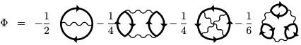
Figure 1: Example of $\Phi$-functional (Stefanucci and van Leeuwen, 2013)

on Fig. 1, where thick arrows denote the Green functions $G(1,2)$ and wiggled lines stand for the particle-particle interaction ${\cal W}(1,2)$ (Stefanucci and van Leeuwen, 2013). For a given $\Phi[G]$, the corresponding self energy is defined as the following functional derivative

$$\Sigma_{{\rm xc}}(1,2)=\frac{\delta\Phi}{\delta G(2,1)}.$$ (29)

Approximations generated via this procedure are called $\Phi$-derivable.

To prove that a $\Phi$-derivable approximation is conserving one has to look on symmetries of the underlying $\Phi$-functional. In particular the condition Eq. (27) is a consequence of the gauge invariance. By construction, any diagram for $\Phi[G]$ is invariant with respect to the following replacement $G(1,2)\mapsto e^{i\Lambda(1)}G(1,2)e^{-i\Lambda(2)}$ where $\Lambda({\bf r},t)$ is an arbitrary function. By requiring that $\Phi[G]$ is unchanged under the corresponding infinitesimal variation, $G(1,2)\mapsto G(1,2)+\delta G(1,2)$ with $\delta G(1,2)=i[\Lambda(1)-\Lambda(2)]G(1,2)$, and using the definition of Eq. (29) we immediately obtain Eq. (27).

Obviously, the gauge invariance of the diagrams for $\Phi[G]$ does not depend on a specific form of the particle-particle interaction ${\cal W}(1,2)$ (only the space-time locality of vertices where two Green functions meet is important). Therefore the modification of the interaction by the cavity photons does not influence the standard arguments and we can safely conclude that $\Phi$-derivable approximations still conserve the number of particles in the presence of quantum electromagnetic field in cavity-QED. In contrast, the situation with the momentum/force balance is very different. The standard proof of the momentum conservation assumes that $\Phi[G]$ is unchanged under a time-dependent shift of space arguments of the Green function $G({\bf r}_{1},t_{1};{\bf r}_{2},t_{2})\mapsto G({\bf r}_{1}+{\bf u}(t_{1}),t_{1};{\bf r}_{2}+{\bf u}(t_{2}),t_{2})$. However, this is only true for an instantaneous translation invariant particle-particle interaction ${\cal W}(1,2)=W({\bf r}_{1}-{\bf r}_{2})\delta(t_{1}-t_{2})$ that implies a Newton third law, $\nabla_{1}W({\bf r}_{1},{\bf r}_{2})=-\nabla_{2}W({\bf r}_{1},{\bf r}_{2})$. The coupling to cavity modes breaks this property by producing an additional photon-exchange interaction given by the second term in Eq. (26). Below I will show how to generalize the proof and demonstrate that the $\Phi$-derivable approximations are consistent with the zero xc force for a more general class of particle-particle interactions, including the one of Eq. (26).

First I notice that by construction $\Phi[G,{\cal W}]$ is a functional of the Green function $G$ and the interaction ${\cal W}$. Another simple observation is that, irrespectively of a specific form of interaction, the $\Phi$-functional is unchanged if we perform a simultaneous shift of space arguments both in $G(1,2)$ and in ${\cal W}(1,2)$,

$$G({\bf r}_{1},t_{1};{\bf r}_{2},t_{2})\mapsto G({\bf r}_{1}+{\bf u}(t_{1}),t_{1};{\bf r}_{2}+{\bf u}(t_{2}),t_{2})$$ ,

$${\cal W}({\bf r}_{1},t_{1};{\bf r}_{2},t_{2})\mapsto{\cal W}({\bf r}_{1}+{\bf u}(t_{1}),t_{1};{\bf r}_{2}+{\bf u}(t_{2}),t_{2})$$ .

The reason for the invariance is the space integration in all vertices in each diagram for a given approximate $\Phi$-functional. Because of this invariance a variation $\delta\Phi$ generated by an infinitesimal translation of spatial arguments of $G$ and ${\cal W}$ should vanish,

$$\int d2\left[\frac{\delta\Phi[G,{\cal W}]}{\delta G(1,2)}\delta G(1,2)+\frac{\delta\Phi[G,{\cal W}]}{\delta{\cal W}(1,2)}\delta{\cal W}(1,2)\right]=0,$$ (30)

where the variations of the two point functions are defined as $\delta F(1,2)={\bf u}(t_{1})\nabla_{1}F(1,2)+{\bf u}(t_{2})\nabla_{2}F(1,2)$. The functional derivative in first term in Eq. (30) is by definition the xc self energy $\Sigma_{{\rm xc}}$ of Eq. (29). By a direct inspection of diagrams the functional derivative in the second terms is easily recognized as the density response function $\chi(1,2)$ (Almbladh et al., 1999; Stefanucci and van Leeuwen, 2013),

$$\frac{\delta\Phi[G,{\cal W}]}{\delta{\cal W}(1,2)}=-\frac{1}{2}\chi(1,2).$$ (31)

Using the above identification of the functional derivatives one can rewrite the identity of Eq. (30) in the following form

$$\int d{\bf r}_{1}d2\left[\Sigma_{{\rm xc}}(1,2)\nabla_{1}G(2,1)-G(1,2)\nabla_{1}\Sigma_{{\rm xc}}(2,1)\right]$$

$$=\frac{1}{2}\int\int d{\bf r}_{1}d2\left[\chi(1,2)\nabla_{1}{\cal W}(2,1)+\nabla_{1}{\cal W}(1,2)\chi(2,1)\right]$$ (32)

where the left and the right hand sides correspond, respectively, to the first and the second terms in Eq. (30). The left hand side in Eq. (32) coincides with the left hand side in Eq. (28). Hence the zero xc force condition is satisfied if the right hand side in the above Eq. (32) vanishes. It obviously vanishes for an instantaneous translation invariant interaction of the form ${\cal W}(1,2)=W({\bf r}_{1}-{\bf r}_{2})\delta(t_{1}-t_{2})$ which satisfies the Newton’s third law. There is however another possibility for the interaction to nullify the right hand side in Eq. (32). Notice that because of the gauge invariance the response function $\chi(1,2)$ satisfies the following identity $\int d{\bf r}_{1}\chi(1,2)=\int d{\bf r}_{2}\chi(1,2)=0$, which guarantees the absence of the density response generated by a spatially uniform scalar potential. Using this property we find that the right hand side in Eq. (32) also vanishes for a biliner interaction of the form ${\cal W}(1,2)=r_{1}^{i}{\cal D}^{ij}(t_{1},t_{2})r_{2}^{j}$, where ${\cal D}^{ij}(t_{1},t_{2})$ is an arbitrary function of only time variables. Therefore a generic particle-particle interaction consistent with the zero xc force condition of Eq. (28) is the following,

$${\cal W}(1,2)=W({\bf r}_{1}-{\bf r}_{2})\delta(t_{1}-t_{2})+r_{1}^{i}{\cal D}^{ij}(t_{1},t_{2})r_{2}^{j}.$$ (33)

This is exactly the form of the particle-particle interaction we have found for the cavity-QED, see Eq. (26). Specifically for the many-electron system interacting with long wavelength cavity photons $W({\bf r}_{1}-{\bf r}_{2})=W_{C}(|{\bf r}_{1}-{\bf r}_{2}|)$ is the Coulomb interaction potential, and ${\cal D}^{ij}(t_{1},t_{2})=\sum_{\alpha}\lambda_{\alpha}^{i}{\cal D}_{\alpha}(t_{1}-t_{2})\lambda_{\alpha}^{j}$ is the electric field propagator for the cavity photons.

The most important conclusion is that despite the coupling to quantum cavity modes breaks the Newton’s third law, all $\Phi$-derivable approximations are still both number- and momentum-conserving.

III.2 Time-dependent density functional theory

In this subsection the previously obtained results will be applied to the construction of conserving approximations for xc potential in the QED extension of TDDFT.

I start with a brief review of QED-TDDFT in a form proposed in Ref. (Tokatly, 2013) and further elaborated in Ref. (Ruggenthaler et al., 2014). Generically QED-TDDFT relies on the following mapping theorem (Tokatly, 2013). The time-dependent many-body wave function $|\Psi(t)\rangle$ of the electron-photon system and the external one-particle potential $V({\bf r},t)$ are unique functionals of the initial state $|\Psi_{0}\rangle$, the electron density $n({\bf r},t)$ and the expectation values $Q_{\alpha}(t)$ of the displacement amplitudes. This statement allows us to calculate the basics observables, $n({\bf r},t)$ and $Q_{\alpha}(t)$, by solving a system of self-consistent Kohn-Sham-Maxwell equations for a set of one-particle KS orbitals $\phi_{i}({\bf r},t)$ and the displacement amplitudes $Q_{\alpha}(t)$:

$$i\partial_{t}\phi_{i} =-\frac{\nabla^{2}}{2m}\phi_{i}+\Big{[}V_{S}+\sum_{\alpha}(\omega_{\alpha}Q_{\alpha}-\bm{\lambda_{\alpha}}{\bf R})\bm{\lambda}_{\alpha}{\bf r}\Big{]}\phi_{i}$$ (34)

$$\partial_{t}^{2}Q_{\alpha}+\omega_{\alpha}^{2}Q_{\alpha}-\omega_{\alpha}\bm{\lambda}_{\alpha}{\bf R}=0.$$ (35)

Here the KS potential $V_{S}({\bf r},t)$ is a sum of the external potential $V({\bf r},t)$, the Hartree potential $V_{H}({\bf r},t)$, and the xc potential $V_{{\rm xc}}({\bf r},t)$,

$$V_{S}({\bf r},t)=V({\bf r},t)+V_{H}[n]({\bf r},t)+V_{{\rm xc}}[n,Q]({\bf r},t).$$ (36)

The xc potential is a functional of the basic observables $V_{{\rm xc}}[n,Q]$ which encodes all complicated many-body effects. It is adjusted in such a way that exact electron density is reproduced in the system of noninteracting KS particles, $n({\bf r},t)=\sum_{\alpha=1}^{N}|\phi_{i}({\bf r},t)|^{2}$. In has been shown in Ref. (Tokatly, 2013) that similarly to the usual TDDFT (Marques et al., 2012; Ullrich, 2012) the xc potential of QED-TDDFT satisfies the zero force condition

$$\int n({\bf r},t)\nabla V_{{\rm xc}}({\bf r},t)d{\bf r}=0.$$ (37)

Clearly this condition is a direct consequence of the conservations laws derived in Sec.II.3. In fact, Eq. (37) ensures the correct global momentum balance in the coupled electron-photon system. It is worth noting that in the KS formulation of any TDDFT the continuity equation is satisfied automatically.

Any practical application of TDDFT requires approximations for the xc potential. In the standard TDDFT a general scheme of constructing conserving optimized effective potential (OEP) approximations for $V_{{\rm xc}}$ has been proposed in Ref. (von Barth et al., 2005). I will show that this scheme can be easily adopted to QED-TDDFT and prove that here it also produces conserving xc potentials.

Following the idea of Ref. (von Barth et al., 2005) I consider an approximate $\Phi$-functional of MBPT, but evaluate it at the KS Green function $\Phi[G_{s},{\cal W}]$, where the KS Green function is the one-particle propagator related to the KS Hamiltonian in Eq. (34). Because of the density-potential mapping $G_{s}[n]$ is a functional of the electron density. Therefore the above $\Phi$-functional can be also regarded as a functional of the density and the particle-particle interaction, $\Phi[G_{s},{\cal W}]=\tilde{\Phi}[n,{\cal W}]$. Importantly, the $\Phi$-functional depends on $n$ only via $G_{s}$. The xc potential is now defined as follows (von Barth et al., 2005)

$$V_{{\rm xc}}({\bf r},t)=\frac{\delta\tilde{\Phi}[n,{\cal W}]}{\delta n({\bf r},t)}.$$ (38)

The level of OEP approximation in this scheme depends on the diagrams taken into account in $\Phi[G_{s},{\cal W}]$.

The first step in proving that xc potential of Eq. (38) is conserving is to analyze the symmetry of the functional $\tilde{\Phi}[n,{\cal W}]$. Let us shift the spatial argument of the density by a time-dependent amount $n({\bf r}+{\bf u}(t),t)$. This will generate the corresponding shift of arguments in the KS Green function $G_{s}({\bf r}_{1},t_{1};{\bf r}_{2},t_{2})\mapsto G_{s}({\bf r}_{1}+{\bf u}(t_{1}),t_{1};{\bf r}_{2}+{\bf u}(t_{2}),t_{2})$. If we simultaneously perform a similar shift in the particle-particle interaction ${\cal W}({\bf r}_{1},t_{1};{\bf r}_{2},t_{2})\mapsto{\cal W}({\bf r}_{1}+{\bf u}(t_{1}),t_{1};{\bf r}_{2}+{\bf u}(t_{2}),t_{2})$, then, in full analogy with the discussion in Sec.III.1, the $\Phi$-functional will remain unchanged. By requiring the invariance of $\Phi[G_{s},{\cal W}]=\tilde{\Phi}[n,{\cal W}]$ with respect to the infinitesimal version of the above shift and performing calculations similar to those in the previous section we arrive at the following identity,

$$\qquad-\int n({\bf r}_{1},t_{1})\nabla V_{{\rm xc}}({\bf r}_{1},t_{1})d{\bf r}_{1}$$ (39)

$$= \frac{1}{2}\int\int d{\bf r}_{1}d2\left[\tilde{\chi}(1,2)\nabla_{1}{\cal W}(2,1)+\nabla_{1}{\cal W}(1,2)\tilde{\chi}(2,1)\right].$$

Here $\tilde{\chi}(2,1)$ is defined similarly to Eq.(31), but with the $\Phi$-functional evaluated at the KS Green function,

$$\frac{\delta\Phi[G_{s},{\cal W}]}{\delta{\cal W}(1,2)}=-\frac{1}{2}\tilde{\chi}(1,2).$$ (40)

The function $\tilde{\chi}(2,1)$ is not the density response function of our physical system. However, by construction it is given by the density response diagrams constructed from the physical interaction ${\cal W}$ and the KS Green $G_{s}$ that is a legitimate one-particle propagator. Therefore $\tilde{\chi}(2,1)$ obeys all fundamental properties of the density response function, in particular $\int d{\bf r}_{1}\tilde{\chi}(1,2)=\int d{\bf r}_{2}\tilde{\chi}(1,2)=0$. Therefore using the same reasoning as in Sec.III.1 we conclude that the right hand side in Eq.(39) vanishes if the particle-particle interaction has a generic form of Eq.(33). In other words I have demonstrated that the described cavity-QED generalization of the OEP construction generates conserving approximations for the xc potential.

Recently an OEP approximation based on the first order xc self energy has been proposed for QED-TDDFT (Pellegrini et al., 2015). A good performance of this approximation has been already demonstrated in several publications (Pellegrini et al., 2015; Flick et al., 2017a, 2018a), however it remained unclear whether it satisfies the fundamental zero force theorem. In terms of the $\Phi$-functional the OEP $V_{{\rm xc}}$ of Ref.(Pellegrini et al., 2015) is generated by the first diagram on Fig.1. Hence the results of the present section imply that this approximation is perfectly conserving.

IV conclusion

In conclusion, by considering the many-body problem for electronic systems strongly coupled to the cavity photon modes I derived the electron force balance equation, and analyzed the exact conditions imposed by this equation on approximate many-body approaches to the cavity-QED. The correct momentum balance in the combined system is guarantied if a properly defined global xc force exerted on electrons from the photonic subsystem vanishes. This condition is similar to the momentum conservability in the standard many-body theory. To construct approximations which fulfill the zero xc force constraint in the frameworks of MBPT and OEP QED-TDDFT I generalized the concepts of $\Phi$-functional and $\Phi$-derivable approximations. In the case of cavity-QED the conservability of $\Phi$-derivable approximations is not as trivial as it may appear on the first sight. The reason is that the exchange by the long wavelength cavity photons induces an effective electron-electron interaction violating the Newton’s third law, which can be traced back to the momentum transfer between the electronic and photonic subsystems. Nonetheless, the concept of conserving approximations can be introduced and all $\Phi$-derivable approximations remain conserving as long as the dipole approximation is valid for the electron-photon coupling (which is the case in most experimentally relevant situations). In particular, this result implies that the recently proposed first order OEP xc potential for QED-TDDFT (Pellegrini et al., 2015) is conserving.

An interesting observation is that $\Phi$-derivable approximations are conserving independently on the specific form of the electric field propagator ${\cal D}^{ij}(t_{1},t_{2})$ in Eq.(33). This suggests a natural and simple way to improve/generalize the OEP of Ref.(Pellegrini et al., 2015) without introducing extra numerical complexity. In the genuine first order OEP one uses the bare photon propagator in the effective interaction, which obviously misses the renormalization of the cavity photons. However the photon renormalization effects can be easily mimicked without breaking the momentum balance by replacing the bare propagator with an effective one constructed phenomenologically on physical grounds, or imported form a simplified solvable system. It would be interesting to explore this possibility in the future.