Evolution of galactic magnetic fields

Abstract

We study the cosmic evolution of the magnetic fields of a large sample of spiral galaxies in a cosmologically representative volume by employing a semi-analytic galaxy formation model and numerical dynamo solver in tandem. We start by deriving time- and radius-dependent galaxy properties using the galform galaxy formation model, which are then fed into the nonlinear mean-field dynamo equations. These are solved to give the large-scale (mean) field as a function of time and galactocentric radius for a thin disc, assuming axial symmetry. A simple prescription for the evolution of the small-scale (random) magnetic field component is also adopted. We find that, while most massive galaxies are predicted to have large-scale magnetic fields at redshift $z=0$, a significant fraction of them is expected to contain negligible large-scale field. Our model indicates that, for most of the galaxies containing large-scale magnetic fields today, the mean-field dynamo becomes active at $z<3$. Moreover, the typical magnetic field strength at any given galactic stellar mass is predicted to decline with time up until the present epoch, in agreement with our earlier results. We compute the radial profiles of pitch angle, and find broad agreement with observational data for nearby galaxies.

1 Introduction

Galactic dynamo theory has had significant success in explaining the properties of the magnetic fields of nearby galaxies (Ruzmaikin et al., 1988; Brandenburg et al., 1992, 1993; Beck et al., 1996; Widrow, 2002; Shukurov, 2005, 2007; Moss et al., 2010; Beck & Wielebinski, 2013; Chamandy et al., 2016). The Square Kilometre Array and other new instruments and techniques will provide an opportunity to see further back in time at ever larger resolution and sensitivity (Beck, 2015b; Taylor et al., 2015; Mao et al., 2017). Properties of galactic magnetic fields at high redshifts, albeit in statistically modest samples, have already been probed by observations of Faraday rotation in Ly$\alpha$ and Mg ii absorption systems (Oren & Wolfe, 1995; Bernet et al., 2008; Irwin et al., 2013; Farnes et al., 2014, 2017; Basu et al., 2018, and references therein) and in a gravitationally lensed late-type galaxy at $z\lesssim 1$ (Mao et al., 2017). The CHANG-ES survey has significantly increased the sample in the nearby Universe with radio data of 35 nearby edge-on galaxies (Wiegert et al., 2015).

To provide appropriate theoretical foundations, three crucial ingredients must be added to dynamo models. Firstly, models need to take into account that galaxies change over cosmic time, and that this can happen suddenly because of galaxy mergers. Despite the fact that galaxy formation models are well-developed (Somerville & Davé, 2015), dedicated galactic dynamo studies have assumed, with rare exceptions, that the underlying galactic parameters are constant throughout the evolution of the magnetic field. Secondly, galaxies have a wide range of parameters. In particular, they vary greatly in size and mass, with dwarf galaxies having different properties from Milky Way (MW)-like galaxies, for instance. Yet most dynamo studies have focused on explaining a generic observed feature, or applying a new physical effect, and usually assume the somewhat canonical parameters that are thought to be roughly suitable for the MW and other similar-sized spiral galaxies. Thirdly, theory and observations of galactic magnetic fields need to be advanced beyond the exploration of a relatively small number of specific galaxies to a statistical analysis of large galaxy samples, both in the nearby Universe and at large redshifts. This requires modelling of the statistical distributions of other galactic properties which affect the dynamo. Thus, a dynamo model is needed that follows the evolution of galaxies over cosmic time, is generic enough to be applied to many different types of galaxy, and can produce a large set of simulated galaxies with a realistic distribution of properties, magnetic and otherwise. This is the challenge that this work begins to address.

Previous attempts to model dynamo action in young galaxies focussed on magnetic field evolution using oversimplified models for the evolution of the host galaxy itself. In the first study of this kind, Beck et al. (1994) employed a nonlinear thin-disc mean-field dynamo model for a generic spiral galaxy whose disc thickness decreases with time as the galaxy evolves. These authors show that the large-scale magnetic field can be amplified to a $\,\mu{\rm G}$ strength in 1–$2\,{\rm Gyr}$ and that large-scale magnetic fields in young galaxies are likely to display global reversals in magnetic field direction that can persist until the present day. Arshakian et al. (2009) used order of magnitude estimates based on dynamo theory to investigate the evolution of magnetic fields in prototypical dwarf, MW-like and giant galaxies. Following Beck et al. (1994), they assumed a mean field dynamo operating on a seed provided by the fluctuation (or small-scale) dynamo. Their results indicated that MW-like galaxies could reach $\sim\,\mu{\rm G}$ fields already at $z=3$, and that the mean field dynamo typically started operating when the age of the Universe was of order $1.6\,{\rm Gyr}$.

The first step in incorporating galactic dynamo theory into the hierarchical galaxy formation theory was taken by Rodrigues et al. (2015). There it was assumed that the galactic magnetic field would either reach the strength associated with the dynamo steady state in galaxies that host a strong dynamo or vanish if the dynamo is sub-critical, with galactic properties obtained from a semi-analytic galaxy formation model. Because of the assumption of instantaneous adjustment of magnetic field, many features of magnetic field evolution remained unresolved. Nevertheless, this approach allowed one to appreciate how the choice of galaxy formation model could affect the detailed distribution of magnetic field strengths. It was also shown that a fraction of galaxies may not contain active dynamos (and thus, large-scale magnetic fields) and that the probability of containing a large-scale magnetic field depends on galaxy mass. In particular, a large class of satellite galaxies was identified that are unlikely to host any large-scale magnetic field because of the stripping of their interstellar medium (ISM) despite possessing kinematic properties favourable for the dynamo action. Here we extend this model by resolving the time evolution of magnetic field and show that the main conclusions of Rodrigues et al. (2015) still hold.

The importance of magnetic fields (and cosmic rays) for galactic evolution is now more widely appreciated and there have been many recent attempts to include magnetic fields in cosmological simulations of forming and evolving galaxies (Pakmor & Springel, 2013; Pakmor et al., 2014, 2017; Marinacci et al., 2018). However, these simulations resolve neither the interstellar turbulence (which takes place on scales less than about $0.1\,{\rm kpc}$) nor the galactic discs (typically, $0.2\text{--}0.5\,{\rm kpc}$). Our earlier experience with using the velocity field from such a model, with adaptive mesh refinement at the highest resolution of $24\,{\rm pc}$, as input for a mean-field dynamo model, has demonstrated that even this resolution is not sufficient to obtain a robust model of magnetic field evolution free from extreme sensitivity to parameters (Agertz et al. 2010, unpublished). Such simulations cannot yet reproduce accurately dynamo action in galactic discs and haloes. Analysis similar to that presented here can be performed using any galaxy formation model but only semi-analytic models provide an opportunity to consider large galaxy samples.

Here we develop a framework to compute magnetic properties of spiral galaxies accounting for the formation history of individual galaxies produced by a galaxy formation model. In this paper we consider magnetic fields in galactic discs – the role of galactic haloes will be discussed elsewhere. For each galaxy, we compute the radial distributions of diffuse gas density and scale height, as well as the rotation curve. These are used as inputs for solving the mean-field dynamo equations, thus modelling the evolution of large-scale magnetic fields in the disc. We focus on describing the fiducial model and its most general and robust consequences. For simplicity, our fiducial model neglects the effects of galactic outflows and accretion flows on the evolution of magnetic fields. While we demonstrate that details of magnetic field structure and evolution are sensitive to specific properties of the galaxy formation model, we can also identify physical effects independent of details of a specific galaxy formation model. A systematic exploration of the parameter space as well as detailed observational consequences will be discussed in subsequent papers.

The plan of the paper is as follows. Section 2 presents galaxy formation models that we use and our ISM based on them (Sections 2.1.4–2.1.6). Our implementation of the fluctuation and mean-field dynamos is discussed in Section 2.2. Section 3 contains our results: for magnetic fields in nearby galaxies in Section 3.1, for a population of galaxies selected at $z=0$ for their significant large-scale magnetic field in Section 3.2, and for a galactic population selected at high redshift in Section 3.3. The radial distributions of large-scale magnetic fields in various redshift and galactic mass intervals are discussed in Section 3.4. Our results are put into a broader perspective in Section 4 and summarised in Section 5. Details of calculations can be found in Appendices.

2 The model

2.1 Galactic properties

We use a semi-analytic model of galaxy formation (SAMGF) to derive the evolution of galaxy properties for a large sample of galaxies of various masses and sizes, consisting of over a million galaxies in the stellar mass range ${8\lesssim\log(M_{\star}/\text{M}_{\odot})\lesssim 12}$. In these models, the assembly history of dark matter (DM) structures is first extracted from a cosmological simulation in the form of a DM halo merger tree. The formation and evolution of galaxies is then followed by solving a set of differential equations describing the physical processes involved in the star formation and its regulation (for reviews and references, see Baugh, 2006; Benson, 2010; Somerville & Davé, 2015). A SAMGF produces a large catalogue of global properties (e.g., disc and bulge stellar masses, their gas masses, the disc half-mass radius, assumed to be the same for gas and stars) at any given redshift. From these, using assumptions consistent with those adopted in the SAMGF, we derive radially-dependent properties of the ISM.

2.1.1 Galaxy formation models

We use the galform SAMGF, introduced by Cole et al. (2000) and continually updated since. We compare two published versions of galform: the one described by Lacey et al. (2016, L16 hereafter) and Gonzalez-Perez et al. (2014, G14 hereafter). Both models use halo merger trees from a Millennium-class $N$-body simulation adopting the WMAP7 cosmological parameters (Guo et al., 2013). The main difference between the two SAMGFs are the assumptions regarding the stellar initial mass function (IMF): L16 uses the IMF of Kennicutt (1983) for quiescent galaxies and assumes a top heavy IMF for starburst galaxies, while G14 assumes universally the Kennicutt IMF.

The results presented here correspond to about 7 per cent of the total volume of the cosmological simulation, that contains about ${1.4\times 10^{6}}$ tracked galaxies.

2.1.2 Correction of stellar disc sizes

galform generally overestimates the disc sizes of small-mass galaxies and underestimates the sizes of large-mass galaxies. We follow the same procedure as Rodrigues et al. (2015) and renormalise the half-mass radii, $r_{1/2}$, of galaxies so that the median of the predicted distribution of $r_{1/2}$ matches the observed relation between the galactic half-mass radius and stellar mass at $z=0$ (Lange et al., 2016). This preserves the dispersion of disc sizes and size evolution computed by the model, while enforcing realistic final galaxy sizes.

2.1.3 Morphology of galaxies

We concentrate on magnetic fields in the discs of spiral galaxies. We classify a galaxy as spiral in galform’s output if its bulge mass accounts for less than half of the total stellar mass, $M_{\text{bulge}}/M_{\text{total}}<0.5$.

2.1.4 Angular velocity and rotational shear rate

We reconstruct the rotation curve of each galaxy in agreement with what is used internally by galform: we assume that galactic discs are thin and have an exponential surface density profile, that the galactic bulges have a Hernquist density profile, and that the dark matter haloes have an adiabatically contracted NFW profile (see Appendix A.2 for details).

While the rotation curve $V(r)$ (where $r$ is the galactocentric distance) obtained under these assumptions is realistic away from the galactic centre, the angular velocity of rotation $\widetilde{\Omega}(r)=V(r)/r$ is singular at the rotation axis. We regularise the angular velocity using

$$\Omega(r)=\mathrm{e}^{-(r_{\xi}/r)^{2}}\left[\widetilde{\Omega}(r)-\Omega(r_{\xi})\right]+\Omega(r_{\xi})\,,$$ (1)

where we take $r_{\xi}=0.1\,r_{1/2}$ . The rotational shear rate is obtained as $S(r)=r\partial\Omega/\partial r$. Such a regularisation is compatible with the nature of the mean-field dynamo model used to obtain the large-scale magnetic field as it assumes that the gas disc is thin and thus only applies at $r\gtrsim r_{\xi}$.

2.1.5 ISM turbulence

The turbulence in the ISM is mostly driven by supernova (SN) explosions. We assume that the root-mean-square turbulent speed $v_{\mathrm{0}}$ is equal to the sound speed $c_{\text{s}}$ in the warm gas ($T\simeq 10^{4}\,\text{K}$),

$$v_{\mathrm{0}}=c_{\text{s}}=10\,{\rm km}\,{\rm s}^{-1}\,.$$ (2)

As discussed in Section 2.2.1 of Rodrigues et al. (2015), these quantities are expected to vary little between and within spiral galaxies. This assumption agrees with recent observations in H i and CO (see Mogotsi et al., 2016).

We assume that the turbulent scale is controlled by the size of a supernova remnant when its expansion velocity reduces to the sound speed in the warm gas, which is of order $0.1\,{\rm kpc}$. However, the turbulent scale is limited from above by the half-thickness of the galactic gaseous disc because larger supernova remnants and their clusters break through the disc into the halo. Thus, we adopt for the turbulent scale

$$l_{0}(r)=\min\left[100\,{\rm pc},h(r)\right]\,,$$ (3)

where $h(r)$ is the scale height of the diffuse gas disc.

2.1.6 Diffuse gas density and scale height

galform does not include a detailed description of the ISM. Thus, the radial profiles of the gas volume density $\rho(r)$ and scale height $h(r)$ have to be estimated from the simulated galaxy properties such as the total stellar mass $M_{\star}$ and the total gas mass of the galactic disc $M_{\text{g}}$.

As is done internally in galform for the stellar disc, the surface density of the gaseous disc is assumed to have an exponential radial profile with the same scale length $r_{\mathrm{s}}$, so for both stars and gas the mass surface densities are adopted as

$$\Sigma_{\text{g}}(r)=\frac{M_{\text{g}}}{2\pi r_{\mathrm{s}}^{2}}\mathrm{e}^{-r/r_{\mathrm{s}}}\quad\text{and}\quad\Sigma_{\star}(r)=\frac{M_{\star}}{2\pi r_{\mathrm{s}}^{2}}\mathrm{e}^{-r/r_{\mathrm{s}}}\,,$$ (4)

where $r_{\mathrm{s}}$ is the scale length (which is the same for stars and total gas).

At the level of spatial resolution available in any galaxy formation model, the multi-phase structure of the ISM can only be allowed for in an approximate manner. The large-scale dynamo appears to operate in the warm phase (Evirgen et al., 2017) because the cold gas occupies a negligible fraction of the disc volume whereas the hot phase is unsteady and leaves the disc for the gaseous halo in a fountain outflow or a wind on time scales shorter than the time scale of the mean-field dynamo. Therefore, we adopt for the ISM the density and temperature characteristic of the warm interstellar gas.

Most of the mass of the cold interstellar gas is in molecular form whereas the hot gas contributes negligibly to the gas mass. The total gas mass is therefore separated into the diffuse (warm) and molecular (cold) phases following a procedure similar to that used by Lagos et al. (2011). We compute the ratio of molecular to diffuse gas surface densities $\kappa=\Sigma_{\text{m}}/\Sigma_{\text{d}}$ using the empirical relation found by Blitz & Rosolowsky (2004, 2006) which relates $\kappa$ to the total gas surface density of $\Sigma_{\text{g}}$ and that of stars, $\Sigma_{\star}$ (see Appendix A.1). From $\kappa$, the surface densities of diffuse and molecular gas components are obtained as, respectively,

$$\Sigma_{\text{d}}(r)=\frac{\Sigma_{\mathrm{g}}(r)}{1+\kappa(r)}\quad\text{and}\quad\Sigma_{\text{m}}(r)=\kappa(r)\Sigma_{\mathrm{d}}(r)\,.$$ (5)

Since $\kappa$ is a function of galactocentric distance $r$, the diffuse and molecular gas phases have distinct radial scale lengths that differ from that of the total gas density.

We adopt exponential density profiles in the coordinate $Z$ perpendicular to the disc surface for the diffuse and molecular gas as well as the stars to obtain the volume mass densities:

$$\rho_{\text{d}}=\rho_{\text{d}0}\mathrm{e}^{-Z/h_{\text{d}}}\,,\quad\rho_{\text{m}}=\rho_{\text{m}0}\mathrm{e}^{-Z/h_{\text{m}}}\,,\quad\rho_{\star}=\rho_{\star 0}\mathrm{e}^{-Z/h_{\star}}\,,$$ (6)

where $\rho_{\text{d}0}$, $\rho_{\text{m}0}$ and $\rho_{\star 0}$ are the corresponding mid-plane values. Assuming that the ISM is in the state of statistical hydrostatic equilibrium, this allows us to derive the mid-plane total gas pressure profile as (see Appendix A.3.1 for the derivation)

$$P(r)= \frac{\pi}{2}G\,\Sigma_{\text{d}}(r)\left\{\Sigma_{\text{d}}(r)\left[1+\frac{2\,h_{\text{d}}(r)R_{\text{m}}(r)}{h_{\text{m}}+h_{\text{d}}(r)}\right]+\Sigma_{\star}(r)\frac{2\,h_{\text{d}}(r)}{h_{\star}+h_{\text{d}}(r)}\right\}$$

$$\quad+h_{\text{d}}(r)\Sigma_{\text{d}}(r)\left[\tfrac{3}{2}\Omega^{2}_{\text{b}}(r)+\Omega_{\text{b}}(r)\;S_{\text{b}}(r)\right]$$

$$\quad+h_{\text{d}}(r)\Sigma_{\text{d}}(r)\Omega_{\text{dm}}\left[\tfrac{3}{2}\Omega_{\text{dm}}(r)+S_{\text{dm}}(r)\right],$$ (7)

where $\Omega_{\mathrm{i}}(r)$ and $S_{\mathrm{i}}(r)=r\partial\Omega_{\mathrm{i}}/\partial r$ are the angular speed and shear rate of the component $\text{i}=\text{d,m,$\star$,b,dm}$, for the diffuse and molecular gas, stellar disc, galactic bulge and dark matter, respectively (see Appendix A.2 for details).

The stellar scale height is observed to be approximately constant with $r$ and related to the radial scale length as $h_{\star}=\beta_{\star}r_{\text{s}}$ with $\beta_{\star}\approx 0.1$ (Kregel et al., 2002). The scale height of the molecular gas in the Milky Way is also approximately constant with $h_{\text{m,MW}}\approx 80\,{\rm pc}$ (Cox, 2005; Heyer & Dame, 2015). We assume that this applies to other galaxies, with their molecular gas scale heights scaling with their disc sizes (analogously to the stellar disc): $h_{\text{m}}=\beta_{\text{m}}r_{\text{s}}$, with $\beta_{\text{m}}\approx 0.032$ and $r_{s}\approx 2.5\,{\rm kpc}$ in the MW (Licquia & Newman, 2016).

Altogether, by accounting for all sources of gravitational support, we have expressed in equation (2.1.6) the mid-plane total gas pressure in terms of the scale height, molecular fraction, surface densities and rotation curves. In order to derive the scale height of the diffuse gas, we represent the total pressure (the sum of thermal, turbulent, magnetic and cosmic-ray contributions), as a multiple of the turbulent pressure,

$$P(r)=\zeta\rho_{\text{d}}(r)v_{\mathrm{0}}^{2}\,,$$ (8)

where $\zeta\approx{1.1}$ is obtained by accounting for the non-thermal pressure components assuming various types of equipartition between them (see Appendix A.3.2 for the derivation). Equations (2.1.6) and (8) express the total mid-plane gas pressure in terms of the surface and volume gas densities, respectively, thus allowing us to obtain the scale height of the diffuse gas,

$$h_{\text{d}}(r)=\frac{\Sigma_{\text{d}}(r)}{2\rho_{\text{d}}(r)}\,.$$ (9)

From this point on, unless otherwise stated, we will omit the subscripts ‘d’ in the density and scale height of the diffuse gas. As discussed below, this leads to a form of a galactic flared disc that is fully compatible with H i observations in the MW.

2.2 Galactic magnetic fields

Turbulent dynamo theory can be conveniently separated into fluctuation dynamo theory, which describes the generation of random magnetic fields by random flows on scales smaller than the outer scale of turbulence (the random or small-scale field), and mean-field dynamo theory, which explains the origin of magnetic fields at scales larger than those of turbulence (the mean, large-scale or regular magnetic field). The mean-field dynamo action also leads to the generation of small-scale magnetic fields but these are uniquely related to the mean magnetic field. The two dynamo mechanisms can act independently and their interaction remains a matter of intense study (Brandenburg & Subramanian, 2005, and references therein). Both dynamos are threshold phenomena: the fluctuation dynamo can maintain a random magnetic field when the magnetic Reynolds number $\mathcal{R}_{\mathrm{m}}$ exceeds a certain critical value of order 100 depending on the detailed nature of the plasma flow, whereas the mean-field dynamo amplifies and then sustains a large-scale magnetic field when, in the simplest case, the dynamo number (depending on the rotation and its shear rates, as defined below) exceeds a critical value of order 10 in a thin disc. For galaxies, the magnetic Reynolds number $\mathcal{R}_{\mathrm{m}}$ exceeds the critical value by several orders of magnitude, and thus interstellar turbulence can amplify an arbitrarily weak random magnetic field exponentially on a time scale comparable to or shorter than the eddy-turnover time $l_{\mathrm{0}}/v_{\mathrm{0}}$ of energy-carrying eddies, of order $10\,{\rm Myr}$ in the Solar neighbourhood. On the other hand, the dynamo number in spiral galaxies is not far from its threshold value, and the large-scale dynamo may or may not be active in a given galaxy depending on its rotation properties and the thickness of its gas layer. For both dynamo mechanisms, the magnetic energy density in a steady-state is of the order of the turbulent energy density. We provide below a quantitative discussion of these mechanisms.

In what follows, we represent magnetic and velocity fields as the sums of large-scale and random parts, denoted with a bar and lower-case symbols, respectively:

$$\bm{B}=\overline{\bm{B}}+\bm{b}\,,\qquad\bm{V}=\overline{\bm{V}}+\bm{v}\,,$$ (10)

where $b_{\mathrm{0}}$ and $v_{0}$ are the respective root-mean-square values of the random parts.

2.2.1 Small-scale magnetic field

Random magnetic fields in the ISM of spiral galaxies are produced by the fluctuation dynamo action and, independently, together with the mean magnetic field as a part of the mean-field dynamo mechanism (e.g., Section 7.4.2 in Shukurov, 2007). As in Rodrigues et al. (2015), we assume that the energy density of the random magnetic field is a fraction $f_{B}$ of the interstellar turbulence energy density,

$$b_{\mathrm{0}}=f_{B}B_{\mathrm{eq}}\,,\quad B_{\mathrm{eq}}=(4\pi\rho)^{1/2}v_{0}\,,$$ (11)

where $\rho$ is the diffuse gas density. Our fiducial model takes $f_{B}=0.5$ (Brandenburg & Subramanian, 2005; Basu & Roy, 2013; Rodrigues et al., 2015; Kim & Ostriker, 2015). Theory and simulations of nonlinear fluctuation and mean-field dynamos still cannot provide a more detailed estimate than this.

2.2.2 Mean-field dynamo equations

We use the standard equations of the nonlinear turbulent mean-field dynamo with simplifications appropriate to the thin discs of spiral galaxies. In particular, differential rotation is assumed to be the dominant source of the azimuthal magnetic field (the $\alpha\omega$ approximation – Ruzmaikin et al., 1988) and derivatives of $\overline{\bm{B}}$ along the $Z$-axis perpendicular to the disc mid-plane are replaced by appropriate ratios involving the scale height of the diffuse gas (the no-$Z$ approximation – Subramanian & Mestel, 1993; Moss, 1995; Phillips, 2001; Chamandy et al., 2014). Apart from differential rotation, we include the outflow at a speed $V_{Z}$. In cylindrical coordinates $(r,\phi,Z)$ centred at the galactic centre with the $Z$-axis aligned with the galactic rotation axis, equations for the radial and azimuthal components of the mean magnetic field reduce to

$$\frac{\partial\overline{B}_{r}}{\partial t}= -\frac{V_{Z}\overline{B}_{r}}{2h}-\frac{2\alpha\overline{B}_{\phi}}{\pi h}+\eta\left\{-\frac{\pi^{2}\overline{B}_{r}}{4h^{2}}+\frac{\partial}{\partial r}\left[\frac{1}{r}\frac{\partial(r\overline{B}_{r})}{\partial r}\right]\right\}\,,$$ (12)

$$\frac{\partial\overline{B}_{\phi}}{\partial t}= -\frac{V_{Z}\overline{B}_{\phi}}{2h}+S\overline{B}_{r}+\eta\left\{-\frac{\pi^{2}\overline{B}_{\phi}}{4h^{2}}+\frac{\partial}{\partial r}\left[\frac{1}{r}\frac{\partial(r\overline{B}_{\phi})}{\partial r}\right]\right\}$$

$$+\frac{\partial\eta}{\partial r}\left(\frac{\partial\overline{B}_{\phi}}{\partial r}+\frac{\overline{B}_{\phi}}{r}\right)+f\,,$$ (13)

where $h(r)$ is the scale height profile obtained in Section 2.1.6, $S(r)$ is the shear rate profile, and $\alpha(r)=\alpha_{\mathrm{k}}(r)+\alpha_{\mathrm{m}}(r)$, with $\alpha_{\mathrm{k}}$ representing the effect of the background mean helicity of interstellar turbulence and $\alpha_{\mathrm{m}}$ the modification of the mean helicity induced by the magnetic field (Pouquet et al., 1976; Kleeorin & Ruzmaikin, 1982; Gruzinov & Diamond, 1994; Bhattacharjee & Yuan, 1995). The following equation for $\alpha_{\mathrm{m}}$ closes the system of equations by allowing for the nonlinear back-reaction of the mean magnetic field on the turbulence (e.g. Kleeorin et al., 2002; Blackman & Field, 2002; Shukurov et al., 2006):

$$\frac{\partial\alpha_{\mathrm{m}}}{\partial t}= -\frac{2\eta}{l_{\mathrm{0}}^{2}B_{\mathrm{eq}}^{2}}\left[\alpha(\overline{B}_{r}^{2}+\overline{B}_{\phi}^{2})+\frac{3\eta}{h}\sqrt{\frac{|D|}{\pi^{3}}}\overline{B}_{r}\overline{B}_{\phi}\right]-\frac{V_{Z}\alpha_{\mathrm{m}}}{h}$$

$$+R_{\kappa}\eta\left[-\frac{\pi^{2}\alpha_{\mathrm{m}}}{h^{2}}+\frac{1}{r}\frac{\partial}{\partial r}\left(r\frac{\partial\alpha_{\mathrm{m}}}{\partial r}\right)\right]+R_{\kappa}\frac{\partial\eta}{\partial r}\frac{\partial\alpha_{\mathrm{m}}}{\partial r}\,.$$ (14)

The $Z$-component of $\overline{\bm{B}}$ can be obtained either from the corresponding component of the dynamo equation (not shown) or, equivalently, from the solenoidality condition $\nabla\cdot\overline{\bm{B}}=0$. Derivation and detailed discussion of these equations and their solutions can be found in Chamandy et al. (2013, 2014) and Chamandy (2016).

The source term $f$ in equation (2.2.2) (its form is derived in Section 2.2.3) is designed to model the statistical contribution of the random magnetic field to the mean-field equation: the mean value of $\boldsymbol{b}$ only vanishes in infinite space but remains significant in the finite volume of a galactic disc.

The background $\alpha$-effect $\alpha_{\mathrm{k}}$ is estimated as

$$\alpha_{\mathrm{k}}=\min\left(\frac{l_{\mathrm{0}}^{2}(r)\Omega(r)}{h(r)},v_{\mathrm{0}}\right)\,,$$ (15)

where the upper limit $v_{\mathrm{0}}$ can be reached in the central parts of galaxies where $\Omega$ is large and $h$ is small, but this rarely happens.

The turbulent magnetic diffusivity is estimated from the mixing length theory as

$$\eta=\tfrac{1}{3}l_{\mathrm{0}}v_{\mathrm{0}}\,.$$ (16)

The microscopic diffusion has been neglected in equations (12)–(2.2.2), which is appropriate given that $\mathcal{R}_{\mathrm{m}}$ is large. The diffusive flux of magnetic helicity within the disc and through the disc surface into the halo is characterised by the parameter $R_{\kappa}$ which we assume to be equal to unity corresponding to equal turbulent diffusivities of magnetic field and helicity (for details, see Chamandy et al., 2014). Since the diffusive flux of magnetic helicity is expected to dominate over the advective flux in the disc (see Section 4.7 of Rodrigues et al., 2015), we neglected the effect of outflows on the magnetic field in the fiducial model we present here.

The intensity of the mean-field dynamo action in the $\alpha\omega$ approximation is controlled by the dynamo number $D$, defined in terms of the nonlinear $\alpha$-effect $\alpha=\alpha_{\mathrm{k}}+\alpha_{\mathrm{m}}$ as

$$D=\left(\alpha_{\mathrm{k}}+\alpha_{\mathrm{m}}\right)\frac{h^{3}S}{\eta^{2}}\,.$$ (17)

We also use the ‘kinematic’ dynamo number defined similarly but for the $\alpha$-effect unaffected by magnetic field,

$$D_{\mathrm{k}}=\alpha_{\mathrm{k}}\frac{h^{3}S}{\eta^{2}}\,.$$ (18)

$D_{\mathrm{k}}$ characterises the ability of a galaxy to launch the mean-field dynamo and contributes to the control of the steady-state strength of the magnetic field, whereas $D$ is approximately equal to $D_{\mathrm{k}}$ when $B\ll B_{\mathrm{eq}}$, and approaches the critical (threshold) values as the dynamo saturates. Both $D$ and $D_{\mathrm{k}}$ are functions of $r$. For the dynamo to be active in a given range of $r$, $D(r)/D_{\mathrm{c}}(r)$ should exceed unity. Since $\alpha_{\mathrm{k}}$ and $\alpha_{\mathrm{m}}$ normally have opposite signs, both $|\alpha|=|\alpha_{\mathrm{k}}+\alpha_{\mathrm{m}}|$ and $|D|$ decrease as magnetic field grows, leading to saturation of the dynamo action and the establishment of a quasi-steady state in which $D(r)/D_{\mathrm{c}}(r)\approx 1$. In this state, the magnetic field is subject to secular variation due to the evolutionary variation of galactic parameters. When $|D|$ decreases below the threshold value $|D_{\mathrm{c}}|$ of order 10 in a thin disc, magnetic field growth is halted and further decrease in $|D|$ leads to the decay of the mean magnetic field at a rate comparable to but lower than the inverse turbulent diffusion time across the disc. The term $f$ in equation (2.2.2) prevents the mean magnetic field from decreasing below the (low) strength that corresponds to the average strength of the random magnetic field in the finite galactic volume as discussed in Section 2.2.3. This weak mean magnetic field serves as a seed for the dynamo action should $|D_{\mathrm{k}}|$ become supercritical again due to the evolution of the galaxy.

Our dynamo model allows for periods of active dynamo action as well as periods of magnetic field decay depending on the nature of the galactic evolution. In particular, we assume that major mergers (i.e., those where the ratio of the merging stellar masses exceeds 0.3) lead to a dispersal of the galactic gaseous discs and their magnetic fields. The mean-field dynamo action can resume after such a merger if $|D_{\mathrm{k}}|>|D_{\mathrm{c}}|$ in the newly formed galaxy but it starts with a weak seed magnetic field.

2.2.3 Random magnetic field and the mean-field dynamo

The spectrum of the fluctuating magnetic field discussed in Section 2.2.1 has a tail extending to small wave numbers. Moreover, averaging of the magnetic fluctuations in a finite volume of the galactic disc does not vanish but rather scales as $N^{-1/2}$, where $N$ is the number of correlation cells of $\boldsymbol{b}$ in the disc volume (Section VII.14 in Ruzmaikin et al., 1988). This statistical large-scale tail acts as a seed for the mean-field dynamo action that is supplied constantly and throughout the galactic disc as long as interstellar turbulence keeps generating random magnetic fields. Therefore, it allows an evolving galaxy to launch the mean-field dynamo action again after a possible period of inactivity. For simplicity, we only include the corresponding source term $f$ into the azimuthal component of the dynamo equation (2.2.2). The magnitude of this seed has been estimated by Ruzmaikin et al. (1988) as

$$\widetilde{B}\simeq\tfrac{1}{3}\frac{b_{\mathrm{0}}}{N^{1/2}}\frac{l}{\Delta r}\,,$$ (19)

where $\Delta r$ ($\simeq 2\,{\rm kpc}$) is the radial width of the leading eigenfunction of the mean-field dynamo equation (close to the galactocentric radius where the rotational shear is maximum). This estimate allows for the fact that $\nabla\cdot\boldsymbol{b}=0$. The number of spherical turbulent correlation cells of a radius $l_{\mathrm{0}}$ in a cylindrical shell of a radius $r$ ($\gg\Delta r$), width $\Delta r$ and height $2h$ is estimated as

$$N\simeq\frac{4\pi hr\Delta r}{(4/3)\pi l_{\mathrm{0}}^{3}}=\frac{3hr\Delta r}{l_{\mathrm{0}}^{3}}\,.$$ (20)

To avoid the formal singularity at $r\to 0$, we introduce an exponential truncation at small radii (that only becomes important at $r\ll\Delta r$) and adopt

$$\widetilde{B}(r)=\tfrac{1}{3}\frac{b_{\mathrm{0}}(r)}{N^{1/2}(r)}\frac{l_{\mathrm{0}}(r)}{\Delta r}{\rm e}^{-\Delta r/(2r)}\,.$$ (21)

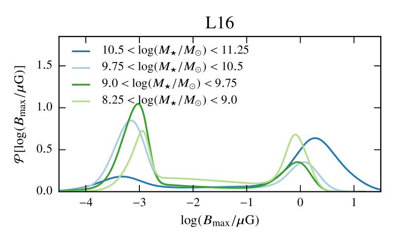
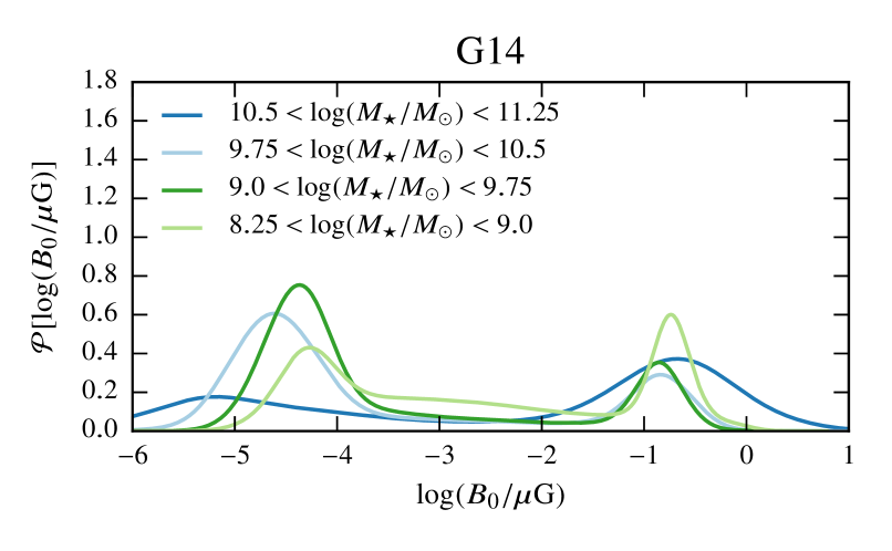
Figure 1: Probability density functions of $\log({B}_{\mathrm{max}})$ and $\log({B}_{0})$ at $z=0$ for spiral galaxies in various mass ranges. The left- and right-hand columns show the results for the G14 and L16 models.

Figure 2: Probability density functions of $\log({B}_{\mathrm{max}})$ at $z=0$ in various galactic stellar mass ranges for the G14 (top panel) and L16 (bottom panel) galaxy formation models. Dashed curves show spiral galaxies with subcritical dynamos at the radius of maximum field strength, i.e., $D_{\mathrm{k}}(r_{\mathrm{max}})/D_{\mathrm{c}}(r_{\mathrm{max}})<1$, while solid curves correspond to galaxies with active dynamos, $D_{\mathrm{k}}(r_{\mathrm{max}})/D_{\mathrm{c}}(r_{\mathrm{max}})>1$.

For $f$, we adopted, after some experimentation, a form that becomes important only for a strongly subcritical dynamo. We choose this term such that, if the dynamo is sub-critical, $\overline{B}_{\phi}$ decays towards a steady state with $\overline{B}_{\phi}\approx\widetilde{B}$. To obtain such a form for $f$, we simultaneously solve equations (12) and (2.2.2) analytically assuming $\partial/\partial t=0$, $\alpha=\alpha_{\mathrm{k}}$ and $\partial/\partial r=0$ (as radial diffusion is sub-dominant in a thin disc). Then $\overline{B}_{\phi}=\widetilde{B}$ leads to

$$f=\frac{\pi^{2}\eta}{4h^{2}}\left(1+\frac{R_{U}}{\pi^{2}}\right)\left(1-\frac{D}{D_{\mathrm{c}}}\right)\widetilde{B}\,,$$ (22)

where

$$R_{U}=\frac{V_{Z}h}{\eta}\,,\quad D_{\mathrm{c}}=-\left(\frac{\pi}{2}\right)^{5}\left(1+\frac{R_{U}}{\pi^{2}}\right)^{2}$$ (23)

are, respectively, the dimensionless outflow velocity (or the corresponding turbulent magnetic Reynolds number), and the critical dynamo number. We have verified that this prescription causes $\overline{B}_{\phi}(r)$ to converge to a profile very close to that of $\widetilde{B}(r)$. If the dynamo is only slightly subcritical, then $\overline{B}_{\phi}$ can be a few times smaller in magnitude than $\widetilde{B}$ in the steady state, due to the radial diffusion neglected in equation (22).

It is unclear how to rigorously prescribe the sign of $\widetilde{B}$: it can vary in both time and space. This variation has observational significance since it can give rise to magnetic field reversals. We applied the following prescription for the choice of the sign of $\widetilde{B}$: it is chosen randomly along $r$ remaining sign-constant within an annulus $10l_{\mathrm{0}}$ wide, and changes randomly over every time interval $10\tau_{\mathrm{0}}=10l_{\mathrm{0}}/v_{\mathrm{0}}$. For the parameter values typical of the Solar neighbourhood, $b_{\mathrm{0}}\simeq 5\,\mu{\rm G}$, $l_{\mathrm{0}}\simeq 0.1\,{\rm kpc}$ and $l_{\mathrm{0}}/v_{\mathrm{0}}\simeq 10\,{\rm Myr}$, $N\simeq 3\times 10^{4}$ and $\widetilde{B}\simeq 5\times 10^{-4}\,\mu{\rm G}$.

2.2.4 Numerical implementation

From the output of the galaxy formation model (galform), 45 fixed-redshift snapshots are extracted, corresponding to the properties of $1.4\times 10^{6}$ galaxies from $z=6$ to $z=0$ (evenly spaced in the logarithm of the cosmological scale factor, which corresponds to time intervals between $100$ and $300\,{\rm Myr}$). The galaxy properties are taken as approximately constant between two consecutive snapshots, and for each interval the angular velocity, density and scale height of diffuse gas are computed for each galaxy as functions of the galactocentric distance $r$.

All radially dependent quantities are computed on an evenly spaced grid spanning the range $0<r\leq 2.7r_{1/2}$, where $r_{1/2}$ is the half-mass radius of the galaxy (including the baryon mass alone). If it is the first snapshot or if $r_{1/2}$ did not increase since the previous snapshot, we use the number of the grid points $n_{r}=55$. If the galaxy had increased in size, the number of grid points is temporarily increased so that $r=2.7r_{1/2}$ can be accommodated using the same radial resolution as in the previous snapshot. After finishing the calculation for a given snapshot, the augmented grid is interpolated back into an $n_{r}$-point grid. For a typical value $r_{1/2}=10\,{\rm kpc}$, the standard grid separation, about $\delta r=0.2\,{\rm kpc}$, is comfortably smaller than the radial scales of the angular velocity, disc scale height, large-scale magnetic field and the seed field $\widetilde{B}$. Since our sample contains a large number of galaxies, significantly larger values of $n_{r}$ can be computationally unaffordable.

Over each time interval between the snapshots, equations (12)–(2.2.2) are solved numerically using a third order Runge–Kutta time stepping and sixth order spatial derivatives (Brandenburg, 2003). The time step $\delta t$ is chosen dynamically to satisfy the following Courant–Friedrichs–Lewy condition based on the advection time scale and magnetic diffusion time across the minimum disc scale height:

$$\delta t=0.16\min\left[\frac{\delta r}{V}\,,\ \frac{\underset{r}{\min}h^{2}(r)}{\eta}\right].$$ (24)

We assume $\overline{B}_{\phi}=\overline{B}_{r}=0$ at both the inner and outer boundaries. We have tested alternative outer boundary conditions $\partial B_{\phi}/\partial r=\partial B_{r}/\partial r=0$ and found negligible impact on the results in the test runs.

3 Results

While our model produces full radial profiles of magnetic properties for each galaxy, it is convenient to have a few diagnostic quantities which can characterise the magnetic field in each galaxy. For this purpose we use the maximum strength of the large-scale magnetic field and the corresponding galactocentric distance $r_{\mathrm{max}}$,

$${B}_{\mathrm{max}}=\max_{r}|\bm{\overline{B}}(r)|=|\bm{\overline{B}}(r_{\mathrm{max}})|\,,$$ (25)

as well as the root-mean-square (rms) large-scale field strength $B_{0}$,

$${B}^{2}_{0}=\frac{\int_{0}^{\infty}|\bm{\overline{B}}(r)|^{2}h(r)\,r\;\mathrm{d}r}{\int_{0}^{\infty}h(r)\,r\;\mathrm{d}r}\,.$$ (26)

3.1 Magnetic fields strength in nearby galaxies

Before discussing magnetic fields in high-redshift galaxies, we evaluate our model at $z=0$ where the results can be compared with observations of nearby galaxies. Figure 1 shows the probability distribution functions (PDFs) of magnetic field strengths in four galactic stellar mass ranges. For both galaxy formation models used and for every mass range, there are two populations, one with mode ${B}_{\mathrm{max}}\simeq 1\,\mu{\rm G}$ and another with mode ${B}_{\mathrm{max}}\simeq 10^{-3}\,\mu{\rm G}$. The large-scale field strength of the latter population is close to the seed field strength $\widetilde{B}$ described in Section 2.2.3. The galaxies in the other population display large-scale magnetic field strengths that are in broad agreement with the observations. The rms magnetic field, $B_{0}$, similarly has a bimodal probability distribution. The two populations are clearly separated by a wide minimum at $10^{-3.5}\lesssim{B}_{0}\lesssim 10^{-1.5}\,\mu{\rm G}$ and we select, for convenience, ${B}_{0}=0.05\,\mu{\rm G}$ as the field strength separating them. The fraction of galaxies with $0.05\lesssim{B}_{0}\lesssim 0.1\,\mu{\rm G}$ is negligible, so, for our present purposes, galaxies with ${B}_{0}>0.05\,\mu{\rm G}$ can be considered to host significant large-scale magnetic fields.

In Fig. 2, the PDFs of ${B}_{\mathrm{max}}$ are shown separately for galaxies with active dynamos (i.e., $D_{\mathrm{k}}/D_{\mathrm{c}}>1$ at ${r=r_{\mathrm{max}}}$) and galaxies incapable of sustaining dynamo action (${D_{\mathrm{k}}/D_{\mathrm{c}}<1}$ at ${r=r_{\mathrm{max}}}$), confirming that the population with the lower field strength in Fig. 1 hosts sub-critical mean-field dynamos.

Figure 3: Fraction of spiral galaxies containing large-scale magnetic field and/or active mean-field dynamos at $z=0$, showed for both L16 (green) and G14 (blue) models. The likelihood that a galaxy hosts a large-scale magnetic fields depends on its stellar mass, with less than 40 per cent of the galaxies with stellar masses about $4\times 10^{9}\text{M}_{\odot}$ containing significant magnetic fields, with the line styles explained in the legend above the figure frame. The red circles with error bars show the fraction of observed galaxies containing large-scale magnetic fields in the compilation of Beck & Wielebinski (2013) and stellar mass data from the S4G catalogue and other sources (see text for details). The vertical bars represent the Poisson errors and the horizontal bars show the width of the logarithmic mass range used. Note that mass ranges are different from those used for the model results in other figures.

There appears to be a connection between the galactic stellar mass and magnetic field strength: most galaxies in the largest-mass range contain strong magnetic fields at $z=0$ while galaxies of a smaller mass host negligible fields; however, this dependence is not monotonic and even smaller galaxies often contain stronger magnetic fields. This is demonstrated in Fig. 3, where we show the fraction of galaxies with a significant field strength exceeding $\widetilde{B}$, ${B}_{\mathrm{max}}>0.05\,\mu{\rm G}$, as a function of the stellar mass at $z=0$. For the L16 model (solid green) this fraction decreases below 40 per cent for $M_{*}\simeq(1\text{--}20)\times 10^{9}\text{M}_{\odot}$ and increases for larger and smaller masses. For the G14 model (solid blue, in Fig. 3), the trend is similar, but the fraction of galaxies with a significant large-scale magnetic field is somewhat smaller. In the same figure, we show the fraction of galaxies where the dynamo is active ($D_{\mathrm{k}}/D_{\mathrm{c}}>1$) at $r=r_{\mathrm{max}}$ depends on the stellar mass. The behaviour is similar to that described above but the fractions are larger, indicating that some of the galaxies did not have enough time to reach the $0.05\,\mu{\rm G}$ threshold even though they currently host an active dynamo.

The circles with error bars in Fig. 3 are based on the data for 89 galaxies compiled by Beck & Wielebinski (2013, arXiv eprint version, updated on 21/02/2018). If a galaxy in their Table 5 contained any indication of magnetic field parallel to the galactic disc (as specified in the ‘Structure’ column), it was counted as a galaxy containing a large-scale magnetic field. Those galaxies listed only as X-shaped, vertical, perpendicular to the plane or exhibiting halo spurs, as well as those listed as having no ordered field, were counted as not containing any large-scale magnetic field. The galactic stellar masses were obtained from the S4G catalogue (Sheth et al., 2010), except for M31 (Chemin et al., 2009), LMC (Kim et al., 1998), NGC 4236 (Pezzulli et al., 2015), NGC 4945, IC 342 (Sofue, 2016), NGC 7331, NGC 2403 and NGC 6946 (de Blok et al., 2008). The data are consistent with a decrease in the fraction of galaxies that host significant large-scale magnetic fields for masses below $10^{10}\text{M}_{\odot}$ but the number of such galaxies is too small (8 and 11 galaxies for the two lowest mass ranges) to reach any confident conclusions. Apart from the largest mass range, both galaxy formation models predict a smaller fraction of galaxies with large-scale magnetic fields than that indicated by observations. It is possible that null detections are under-reported, or that there is selection bias (e.g., galaxies being targeted because they are bright in the radio range), and such biases would tend to enhance the reported detection fraction. On the other hand, it is possible that in some galaxies the large-scale magnetic field was too weak to be detected, yet still above the $0.05\,\mu{\rm G}$ cut-off, which would tend to reduce the detection fraction. Another reason for the discrepancy could be an inaccurate estimation of the galactic stellar disc and bulge masses in the galaxy formation models. These issues will be addressed elsewhere. Nevertheless, it is encouraging that theory and observation agree that a significant fraction of galaxies at $z=0$ do not contain large-scale magnetic fields, and that this fraction appears to be higher for dwarf galaxies than for MW-like galaxies.

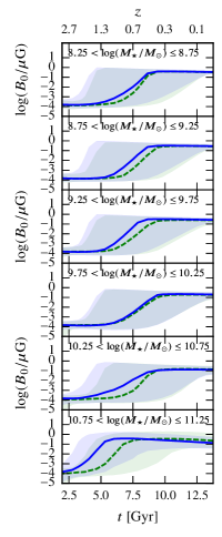
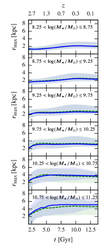
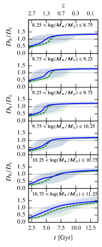
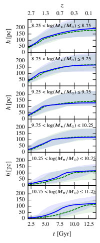
Figure 4: Evolution of (left to right and top to bottom): (i) the rms large-scale magnetic field strength ${B}_{0}$ of equation (26), (ii) the maximum large-scale field strength ${B}_{\mathrm{max}}$ defined in equation (25), (iii) galactocentric radius $r_{\mathrm{max}}$ where $\overline{B}(r_{\mathrm{max}})={B}_{\mathrm{max}}$, and the following quantities at $r=r_{\mathrm{max}}$: (iv) the ratio ${B}_{\mathrm{max}}(r_{\mathrm{max}})/B_{\mathrm{eq}}$, where $B_{\mathrm{eq}}$ corresponds to energy equipartition with interstellar turbulence, equation (11), (v) the ratio of the kinematic dynamo number $D_{\mathrm{k}}(r_{\mathrm{max}})$ of equation (18) to its critical value $D_{\mathrm{c}}(r_{\mathrm{max}})$ of equation (23) (vi) the scale height of the diffuse gas $h(r_{\mathrm{max}})$, (vii) the angular velocity $\Omega(r_{\mathrm{max}})$, and (viii) dimensionless rotational shear rate; $q=1$ for a flat rotation curve and $q=0$ for a solid-body rotation. Only those spiral galaxies are included that have ${B}_{\mathrm{max}}>0.05\,\mu{\rm G}$ at $z=0$ in each stellar mass interval indicated in the legend of each frame. The solid (blue) and dashed (green) curves show the median of the distribution for the L16 and G14 galaxy formation models, respectively, and the shaded areas of matching colour correspond to the interval between the 15th and 85th percentiles.

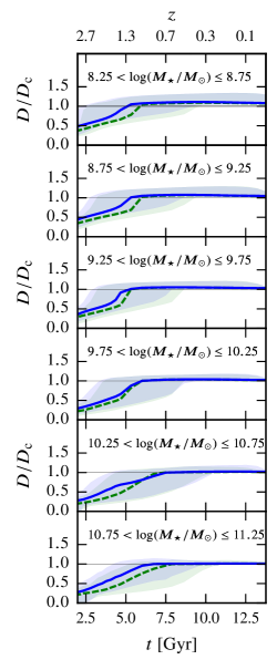
Figure 5: As in Fig. 4 but showing the ratio of the dynamo number affected by magnetic helicity, $D(r_{\mathrm{max}})$ of (17), to $D_{\mathrm{c}}(r_{\mathrm{max}})$.

3.2 Magnetic history of galaxies

In this section we consider in detail the population of galaxies that possess a large-scale magnetic field at $z=0$ to understand when it was amplified to the present-day strength. Figure 4 illustrates the time evolution of the rms and maximum strengths of the mean galactic magnetic fields as well as the derived parameters of the gaseous discs and dynamo number in various mass intervals. Spiral galaxies with ${B}_{\mathrm{max}}>0.05\,\mu{\rm G}$ in six stellar mass ranges were selected at $z=0$, and their evolution was traced back to the beginning of the galform simulation. For most galaxies, the large-scale magnetic field was amplified to the present-day level between $z=1$ and $z=3$. In each mass interval, there is a more or less well-defined epoch, of $\delta z\simeq 1$ in duration, when the magnetic field starts growing and galaxies reach a steady dynamo state after about $8.5\,{\rm Gyr}$ of evolution. The typical radius where the mean magnetic field strength is maximum varies little with time, ranging from $1\lesssim r/\,{\rm kpc}\lesssim 2$ in the smallest stellar mass range, to $2\lesssim r/\,{\rm kpc}\lesssim 7$ for the most massive galaxies. This radius is usually close to that of maximum rotation shear near the turnover radius of a flat rotation curve. The panel showing ${B}_{\mathrm{max}}/B_{\mathrm{eq}}$ indicates that the most massive galaxies tend to have large-scale magnetic fields above equipartition for $z<0.7$, while most galaxies of a smaller stellar mass never quite reach $B_{\mathrm{eq}}$.

The choice of a specific SAMGF has little impact except for the largest mass bin, where, in the L16 model, many galaxies produce large-scale magnetic fields approximately $2\,{\rm Gyr}$ earlier than in G14. The main reason for this difference is the larger rotation rates in the former model.

Given the critical value of the dynamo number $D_{\mathrm{c}}$ (equation 23), the mean-field dynamo activity is controlled by the diffuse gas scale height, $h$, angular velocity, $\Omega$, and shearing rate, $S=r\partial\Omega/\partial r$, as $D\propto h^{2}\Omega S$. The time evolution of each of these quantities at the radius of maximum field strength is shown in Fig. 4. It does not seem that the control of the dynamo activity can be attributed to a single dominant variable. The angular velocity of galactic rotation first decreases with time and then stagnates (as galaxy sizes grow faster than circular velocities perhaps because of the difference in the rates of dark matter and gas accumulation) while the shearing rate $S$ follows the behaviour of $\Omega$ (the ratio $q=-S/\Omega$ at $r=r_{\mathrm{max}}$ is approximately constant in time as shown in the lower-right panel of Fig. 4). Both the reduction in the rate of decrease of $\Omega$ (and $|S|$) and the steady increase of $h$ play a role in the establishment of a supercritical dynamo. This seems to apply to all stellar mass bins and redshifts, though the relative importance of these two factors varies with stellar mass. We also note that the rapid rise of $D/D_{\mathrm{c}}$ and of ${B}_{0}$ occurs earlier for galaxies with higher stellar mass. Moreover, the larger the stellar mass, the less scatter in the time at which this rapid growth phase happens.

Finally, comparing $D_{\mathrm{k}}/D_{\mathrm{c}}$ with $D/D_{\mathrm{c}}$ (the first panel in the bottom row of Fig. 4 and Fig. 5) allows one to appreciate the magnetic contribution to the $\alpha$-effect (the term $\alpha_{\mathrm{m}}$ in equations 12–2.2.2) and the associated quenching of the mean-field dynamo. As expected, the dynamo number modified by the magnetic field gradually approaches the critical value as magnetic field grows, so that $D/D_{\mathrm{c}}\approx 1$ whenever $D_{\mathrm{k}}/D_{\mathrm{c}}>1$.

Figure 6: The variation with redshift (the horizontal axis) of the probability density of the large-scale magnetic field strength (the rms field in the upper and lower panels, and the ratio of the maximum to the equipartition field in the middle panel) of spiral galaxies separated at each redshift into two stellar mass bins, $8.5<\log(M_{\star}/\text{M}_{\odot})<10.5$ (dark blue) and $\log(M_{\star}/\text{M}_{\odot})>10.5$ (light blue). The top two panels are obtained for the L16 model, while the bottom panel illustrates the difference between the L16 (blue) and G14 (green) models for the massive galaxies, $M_{\star}>10^{10.5}\text{M}_{\odot}$, in terms of the rms magnetic field strength.

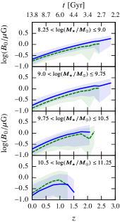
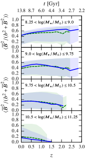
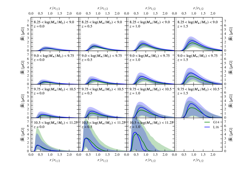
Figure 7: The evolution of magnetic field parameters for galaxies in the mass intervals shown in the legends (from left to right): (i) the fraction of spiral galaxies with ${B}_{\mathrm{max}}>0.1\,\mu{\rm G}$; (ii) the rms large-scale field strength ${B}_{0}$; (iii) magnetic pitch angle at the radius of maximum field, $p(r_{\mathrm{max}})$; and (iv) the ratio of the large-scale to total magnetic field strengths averaged over the galactic disc. The results are shown only for spiral galaxies with significant (exceeding $0.05\,\mu{\rm G}$) large-scale magnetic fields selected by mass at each redshift. The solid (blue) and dashed (green) curves show the median of the distribution for the L16 and G14 models, respectively. The shaded areas correspond to the interval between the 15th and 85th percentiles.

Figure 8: Radial profiles of large-scale magnetic field strength, for different choices of redshift and stellar mass (as indicated in the legends) for galaxies with ${B}_{\mathrm{max}}>0.1\,\mu{\rm G}$. Solid curves represent the median values and shaded areas show the 15th and 85th percentiles.

Figure 9: Pitch angle of the large-scale magnetic field $p=\arctan{\overline{B}_{r}/\overline{B}_{\phi}}$ versus galactocentric radius for different choices of redshift and stellar mass (as indicated in the panel legends) for galaxies with ${B}_{\mathrm{max}}>0.1\,\mu{\rm G}$. Solid curves show median values and shaded areas span the range between the 15th and 85th percentiles (blue for L16 and green for G14). Points with error bars at $z=0$ show observational estimates for M31 , M33, M51, M81, NGC 1566, NGC 253, NGC 6946, IC 342 (red) and barred galaxies NGC 1097 and NGC 1365 (black) (see Chamandy et al., 2016, for references); horizontal error bars represent the radial range to which the estimates belong.

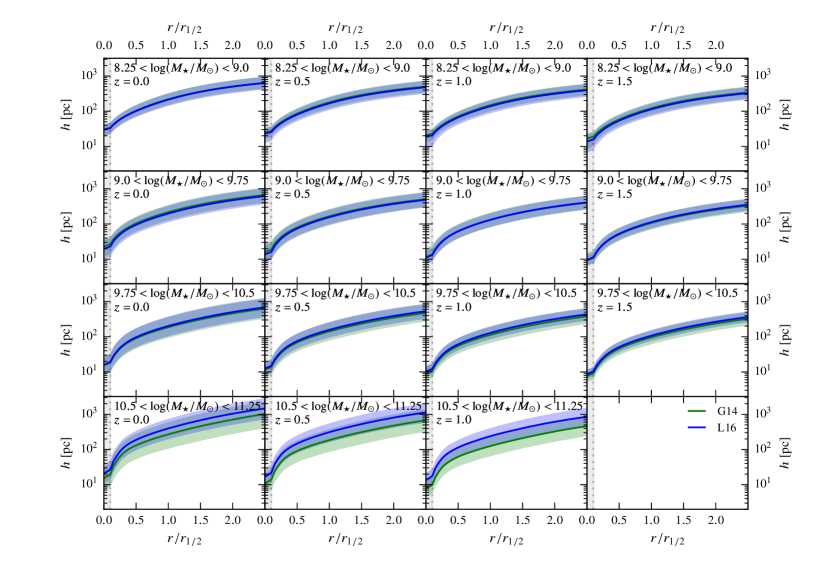
Figure 10: As in Figs 8 and 9 but for the diffuse gas scale height $h$.

3.3 Cosmological evolution of galactic magnetism

The previous section is focused on the evolution of the population of galaxies with significant large-scale magnetic field at redshift $z=0$. These are the galaxies that would be selected for magnetic field studies in the nearby Universe. The sample is obviously biased. To provide a more complete picture, here we consider constructing samples of galaxies from our simulation using criteria characteristic of observations of high-redshift galaxies, e.g., the surface brightness. Since most galactic observables are related to the galactic stellar mass, we use this variable as a proxy for any other observable.

Figure 6 shows how the probability density distributions of the rms and maximum field strengths of the large-scale magnetic field evolve for $0<z<2.5$ for two galactic mass ranges, $8.5<\log(M_{\star}/\text{M}_{\odot})<10.5$ and $\log(M_{\star}/\text{M}_{\odot})>10.5$. At each redshift, a significant fraction of the galaxies have weak magnetic field strengths of order $10^{-4}\,\mu{\rm G}$. The fraction of galaxies which do contain significant large-scale magnetic field decreases with redshift (and increases with time) in agreement with Rodrigues et al. (2015). This suggests that the assumption of Rodrigues et al. (2015), relaxed in this work, that the mean-field dynamo is approximately in a steady state in each galaxy at any given redshift, is fairly robust. This is consistent with the analysis of Section 3.2, where it is shown that once $D/D_{\mathrm{c}}$ has reached unity, it does not deviate very much from that value. If it was common for galaxies to deviate from the steady state once they produced significant large-scale fields, then this would have resulted in more scatter about $D/D_{\mathrm{c}}=1$ than what is seen in Fig. 5. The middle panel of Fig. 6 shows the ratio of the maximum field strength to the equipartition field strength – Eq. (11) –, the typical values $B_{\mathrm{max}}/B_{\mathrm{eq}}(r_{\mathrm{max}})$ for the galaxies with significant large-scale fields remain approximately constant, which is expected if the galaxies had reached steady-state.

The top panel of Fig. 6 shows that galaxies with stellar masses $\log(M_{\star}/\text{M}_{\odot})>10.5$ undergo a transition from being devoid of significant large-scale fields at $z=2$ to mostly having significant large-scale fields at $z=1$. Galaxies with $\log(M_{\star}/\text{M}_{\odot})<10.5$, on the other hand, have a very different history. At $z=2.5$, there is already a small but significant fraction of galaxies that contain large-scale fields of order a few $\!\,\mu{\rm G}$. The fraction of galaxies that have significant large-scale fields (the ratio of areas around the local maxima in the probability density) increases steadily with time, whereas for the higher stellar mass population, it increases until $z\simeq 0.5$, after which it remains roughly constant (and even decreases slightly). Thus, the overall evolution tends to be faster for the higher stellar mass population. Furthermore, of those galaxies that host significant large-scale magnetic fields in the lower stellar mass population, the median value is larger than for the more massive galaxies, while the width of the distribution is much narrower.

In the bottom panel of Fig 6, we compare the L16 and G14 models for $\log(M_{\star}/\text{M}_{\odot})>10.5$. The transition redshift after which most of the massive galaxies contain significant large-scale magnetic fields is lower in G14 than in L16. The results for small-mass galaxies are indistinguishable for the two models and have, thus, been omitted.

We found in Section 3.2 that in galaxies that host a large-scale magnetic field, the typical field strength decreases with time in each mass interval considered. This is further illustrated in the second column of Fig. 8 where the galaxies with negligible large-scale magnetic field were removed. Thus, a survey of galaxies selected by mass (or a related quantity) at each redshift would find a strong increase of the typical field strength observed with redshift. However, at higher redshifts, not only does the abundance of galaxies with a certain stellar mass decrease (due to the evolution of the stellar mass function – see, e.g., Fig. 24 in Lacey et al. 2016) but so does the fraction of those which contain significant large-scale magnetic fields (the first column of Fig. 8).

The third panel of Fig. 8 shows the evolution of the magnetic pitch angle, given by $\tan p=\overline{B}_{r}/\overline{B}_{\phi}$ (with $-90^{\circ}<p\leq 90^{\circ}$), that characterises how tightly wound is the large-scale magnetic field spiral (see Chamandy & Taylor, 2015; Chamandy et al., 2016, and references therein). The pitch angle, reported at the radius of maximum magnetic field strength, generally ranges from $-20^{\circ}$ to $-30^{\circ}$ (with negative values corresponding to a trailing spiral). The typical value of $p(r_{\mathrm{max}})$ depends on the galaxy mass, and, in all cases, the median value of $p(r_{\mathrm{max}})$ decreases (becomes more negative) with redshift: magnetic lines become more tightly wound as the galaxy evolves.

The rightmost panel of Fig. 8 shows the evolution of the degree of order in the magnetic field defined as the ratio of the mean to the total magnetic field averaged over the disc surface, $P=\langle\overline{B}^{2}/(\overline{B}^{2}+b_{\mathrm{0}}^{2})\rangle$. This quantity varies significantly with both galactic stellar mass and redshift: massive galaxies have less ordered magnetic fields, $0<P\lesssim 0.6$ with a median of $0.2$ at $z=0$, while the smallest galaxies, $8.25<\log(M_{\star}/\text{M}_{\odot})<9.0$, have $0.2\lesssim P\lesssim 0.8$ with a median of about $0.45$ at $z=0$. Since $P$ is related to the fractional polarisation of synchrotron emission (that can be further reduced by Faraday effects), these results indicate that the fractional polarisation is expected to decrease strongly with redshift if only massive galaxies are selected at each redshift. The opposite trend is expected for galaxies of the lowest stellar mass.

3.4 Radial magnetic profiles

Figures 8 and 9 present the radial profiles of the large-scale magnetic field strength and magnetic pitch angle, respectively. At redshifts $z=0$, $0.5$, $1.0$ and $1.5$, galaxies were selected by mass – in the four intervals shown – and, to account for variations in the sizes of galactic discs, the galactocentric radius is normalised to the half-mass radius of each galaxy, $r_{1/2}$. The grey shaded area along the left-hand vertical axis in each panel indicates the region where the angular velocity is truncated as described in Section 2.1.4. Our model underestimates magnetic field strength in this region because of this truncation; furthermore, the thin-disc and, possibly, $\alpha\omega$ approximations are not justified there (Ruzmaikin et al., 1988; Chamandy, 2016). Large-scale magnetic fields are expected to be strong in the central parts of galaxies.

The half-mass radii of individual nearby galaxies were estimated as $r_{1/2}=0.4R_{25}$, where $R_{25}$ is the radius of the $25\,\text{mag\,arcsec}^{-2}$ isophote from the LEDA database, and the stellar mass was obtained from the S4G (Sheth et al., 2010) catalogue. We have calculated $r_{1/2}/R_{25}$ for 101 galaxies in the 2MASS catalogue to obtain the median and mean values of 0.39 and 0.44, respectively, with the sample standard deviation of 0.16.

Figure 8 shows that the relative radius $r_{\mathrm{max}}/r_{1/2}$ where magnetic field strength is maximum is smaller at lower redshifts in each mass interval, apparently because the turnover radius of galactic rotation curves, where the rotational shear is maximum, decreases with time. There is generally good agreement between the two galaxy formation models, L16 and G14. Galaxies with smaller stellar mass have more extended profiles in the unit of half-mass radius, showing that the magnetic field profile does not scale linearly with the galaxy size. Large-scale magnetic fields are first amplified closer to the galactic centre, where the angular velocity and its shear are larger, and then spread outwards in the form of a magnetic front (Moss et al., 1998; Willis et al., 2004). Thus, our results suggest that the rate of growth of galactic discs is larger than the rate of spread of the magnetic field. Consistently with Figs. 1 and 6, the range of field strengths depends on galaxy stellar mass, being much wider at larger masses.

In the $z=0$ (leftmost) column of Fig. 9, we show observational estimates of the magnetic pitch angles in nearby galaxies compiled by Van Eck et al. (2015) and Chamandy et al. (2016). These data points are supplied with horizontal error bars that show the range of radii where the value was reported by Van Eck et al. (2015). (We note that our estimates of the half-mass radius for nearby galaxies may not be reliable even if they are statistically accurate; this may have affected the observational data points in Fig. 9.) Magnetic pitch angle, shown in Fig. 9, decrease in magnitude with radius, an overall trend consistent with observations (Section 4.6 in Beck, 2015a). The two galaxy formation models used lead to significantly different predictions for the pitch angle profiles of the most massive galaxies, with G14 producing larger $|p|$. At $r/r_{1/2}<1.5$, predictions of the G14 model are marginally consistent with the observations of nearby galaxies while the L16 model predicts somewhat too small values of $|p|$. Better agreement would require more accurate estimates of parameters like $l_{0}$ and $v_{0}$, which are likely to vary within and between galaxies. In addition, other refinements of our dynamo model may improve the agreement, such as accounting for the effects of spiral patterns, galactic outflows and accretion flows (see Chamandy et al., 2016, for a discussion).

The scale height of diffuse gas as shown in Fig. 10 increases with galactocentric radius – the gas disc is flared. At $r/r_{1/2}\gtrsim 0.5$, the scale height increases nearly exponentially, mainly because of the exponential radial decrease in the stellar gravity field. The exponential gas disc flaring agrees with H i observations in the MW (Kalberla & Kerp, 2009, and references therein) and other galaxies. (see e.g. Peters et al., 2017; O’Brien et al., 2010), and lends support to the ISM model in evolving galaxies developed in this paper. Also Chamandy et al. 2016 shows that flaring scale height profiles are necessary in order to explain the observed pitch angles of nearby galaxies using a general mean field dynamo model.

4 Discussion

The seed magnetic field for the mean-field dynamo, estimated as $\widetilde{B}\simeq 5\times 10^{-4}\,\mu{\rm G}$ in Section 2.2.3, is provided by the fluctuation dynamo action of interstellar turbulence. This mechanism to generate random magnetic fields can be active continuously as soon as star formation in an evolving galaxy becomes intense enough to drive pervasive random flows in the interstellar gas. Unlike primordial seed magnetic fields, this mechanism constantly seeds galactic mean-field dynamos and therefore can support re-launching of mean-field dynamo action in galaxies that became temporarily incapable of sustaining mean-field dynamo action in the course of their evolution, e.g., due to the destructive effects of mergers on the galactic rotation and gaseous disc.

The presence of random magnetic fields at all stages of evolution of star-forming galaxies has an important implication for the confinement of cosmic rays. The Larmor radius of a 1 GeV relativistic proton is smaller than the characteristic disc scale height of $200\,{\rm pc}$ in a magnetic field as weak as $10^{-5}\,\mu{\rm G}$. The fluctuation dynamo generates random magnetic fields of a strength comparable to that corresponding to equipartition with the turbulent kinetic energy density, a few microgauss. Therefore, cosmic rays can be efficiently confined to galaxies from the earliest stages of their evolution (Zweibel, 2013). This justifies our inclusion of cosmic ray pressure in the calculation of the gas scale height in hydrostatic equilibrium in Appendix A.3.2 and equation (8).

As Fig. 6 shows, the evolution of galactic large-scale magnetic fields is rather non-trivial: on the one hand, the fraction of galaxies that host such a field increases with time but, on the other hand, the field strength decreases. This has interesting implications for the effects of magnetic field on the stellar feedback on galactic evolution via galactic outflows. As discussed by Evirgen et al. (2019), large-scale magnetic fields produced by dynamo action are effective in quenching galactic outflows, with the dependence of the outflow speed on magnetic field strength fitted by

$$V_{z}\propto\left[1+0.5(\overline{B}/B_{\mathrm{eq}})^{n}\right]^{-1}\,,$$ (27)

with $n$ in the range 3–4 (see also Bendre et al., 2015; Shukurov et al., 2018). The dependence on $\overline{B}$ is strong, implying a very efficient suppression of an outflow. Simulations of the supernova-driven ISM, on which this result relies, do not yet contain cosmic rays; their pressure may make the effect weaker. Nevertheless, the possibility of a strong effect of the galactic mean-field dynamo action on the stellar feedback needs to be considered carefully. Taken at their face value, our results suggest that the outflows can be more readily suppressed at larger redshifts where magnetic field strength is larger. This question requires further analysis.

In every mass range (perhaps except for the most massive galaxies – see Fig. 3), there are galaxies that do not have any significant large-scale magnetic fields. Apart from the statistical scatter in the magnitude of rotation speed and its shear (resulting from the random nature of the evolution of the galactic angular momentum), reflected in the scatter of the kinematic dynamo number $D_{\mathrm{k}}$, galaxy mergers can contribute to disturbing the mean-field dynamo action. In the model that we use, the major mergers are assumed to destroy galactic gaseous discs and disperse magnetic fields, and then the dynamo may be launched again. It is not surprising then that massive galaxies have a wider range of field strengths as they have more complex formation history than galaxies of smaller mass.

The present work focused on the magnetic fields in galactic discs. Galactic discs are much brighter in synchrotron emission than the haloes (Wiegert et al., 2015) and therefore dominate in such observables as the galactic radio luminosity function. On the other hand, the magnetic field in galactic haloes – which was not considered here – may be significant for Faraday rotation measure studies and in detailed radio characterisation of resolved edge-on galaxies, and has been explored in recent works (see e.g. Henriksen et al., 2018). A treatment of the magnetic field in haloes which consistently accounts for the galaxy evolution requires detailed understanding of the magnetised winds produced by galaxies (see Heesen et al., 2018, and references therein) and is the subject of our present active research.

5 Summary and conclusions

We have developed an ISM model for a large sample of more than a million evolving galaxies based on SAMGF and used it to explore statistical properties of galactic dynamos and magnetic fields that they produce. The ISM model includes those ingredients that control fluctuation and mean-field turbulent dynamos, galactic rotation curves and flared gas discs in particular (Figs. 4 and 10). Seed magnetic fields in our model of the galactic mean-field dynamo are continuously replenished by fluctuation dynamo action, which allows the mean-field dynamo to be reactivated after major galactic mergers or other events destructive for galactic discs and their magnetic fields. (This mechanism of galactic seed magnetic field generation is therefore more flexible than primordial mechanisms.) Such disruptions are especially common in the formation history of massive galaxies. As a result, the more massive is a galaxy, the later, on average, it becomes able to support a sustained mean-field dynamo action and a microgauss-strength large-scale magnetic field (Fig. 8).

A significant fraction (dependent on galactic mass) of galaxies possess no large-scale magnetic fields, with a minimum of about 20 per cent for the stellar mass $M_{\star}\simeq 10^{10}\text{M}_{\odot}$ (Figs. 3 and 6), some galaxies cannot support the mean-field dynamo (Fig. 2) because their rotation rate and/or velocity shear is too weak or the gas disc is too thin.

Our results suggest that large-scale magnetic fields can be amplified to a microgauss strength in $2\text{--}3\,{\rm Gyr}$, starting at $z=3\text{--}2$ depending on the galactic mass (Fig. 4). We stress that this time scale is much shorter than the often quoted estimate of $10\,{\rm Gyr}$ (or more) based on estimates only applicable in the Solar neighbourhood of the MW. The galactocentric radius where the large-scale magnetic field is maximum ranges from about $2\,{\rm kpc}$ in low-mass galaxies to $5\,{\rm kpc}$ in massive ones. In general, dynamo action starts later in more massive galaxies (Fig. 8) but this depends subtly on sample selection criteria: for galaxies selected at $z=0$ for their strong magnetic field, the trend is reversed and more massive galaxies produce their magnetic fields earlier (Fig. 4). The differences between magnetic histories of galaxies of various masses are largely due to the differences in their assembly; our model assumes that each major merger disperses galactic gas discs with their magnetic fields, and dynamo action resumes again after such events. This shows that interpretations of either observations or simulations of galactic magnetic fields in high-redshift galaxies require extreme care and attention to sample biases and selection effects.

Another non-trivial aspect of our results is a prediction that the fraction of galaxies with significant large-scale magnetic fields increases with time but the strength of their magnetic fields decreases due to the depletion of interstellar gas as a galaxy evolves (Figs. 6 and 8).

The two versions of the galform galaxy formation model considered (L16 and G14) lead to broadly similar magnetic field forms and evolution patterns but there is some variance too. The most prominent difference is that they predict different fractions of galaxies with strong large-scale magnetic fields (Fig. 6). This and other differences can be used to constrain galaxy formation models using magnetic field observations in statistically representative samples of galaxies, either in the nearby Universe or at high redshifts.

Appendix A Details of the galaxy modelling

A.1 Molecular gas fraction

To compute the molecular fraction of the interstellar gas density, we start by computing a notional pressure profile, $\widetilde{P}(\Sigma_{\star},\Sigma_{\text{g}})$, based on the approximate expression for the mid-plane pressure suggested by Elmegreen (1989),

$$\widetilde{P}(r)=\frac{\pi}{2}G\,\Sigma_{\mathrm{g}}(r)\left[\Sigma_{\mathrm{g}}(r)+\frac{v_{0}}{\sigma_{\star}(r)}\Sigma_{\star}(r)\right]\,,$$ (28)

where $\sigma_{\star}$ is the velocity dispersion of the stellar component, estimated using

$$\sigma_{\star}^{2}=\pi Gh_{\star}\Sigma_{\star}(r)\,,$$ (29)

where the stellar scale height is $h_{\star}=fr_{s}$, with $f\approx 0.137$ (Kregel et al., 2002).

Once $\widetilde{P}(r)$ is known, the fraction of molecular gas can be computed as

$$\kappa(r)=\left[{\widetilde{P}(r)}/{P_{0}}\right]^{\alpha}\,,$$ (30)

where $P_{0}=4.787\times 10^{-12}\,{\rm erg}\,{\rm cm}^{-3}$ and $\alpha=0.92$ were obtained from observations (Blitz & Rosolowsky, 2004, 2006; Leroy et al., 2008).

A.2 Rotation curves

To be able to obtain an accurate solution for the magnetic field, good knowledge of the rotation curve is required. We reconstruct the rotation curve from galform output in the following way. The disc is assumed to be thin and to have an exponential surface density profile, which leads to the following rotation curve (Binney & Tremaine, 2008):

$$V_{\text{disc}}(y)\propto y\left[I_{0}(y)K_{0}(y)-I_{1}(y)K_{1}(y)\right]^{1/2}\,,$$ (31)

where $y=r/(2r_{s})$, and $I_{n}$ and $K_{n}$ are modified Bessel functions of the first and second kinds, respectively, and $r_{s}$ is the disc scale radius.

We assume the mass in the bulge follows a Hernquist (1990) profile which leads to the following circular velocity profile

$$V_{\text{b}}\propto\sqrt{\frac{r}{(r+r_{\text{b}})^{2}}}\,,$$ (32)

where $r_{\text{b}}$ is a characteristic radius.

Finally the dark matter halo is assumed to follow an NFW profile, which leads to a rotation curve (Mo et al., 2010),

$$V_{0}(r)=V_{\text{vir}}\left[\frac{1}{x}\frac{\ln(1+cx)-cx/(1+c)}{\ln(1+c)-c/(1+c)}\right]\,,$$ (33)

where $x=r/r_{\text{vir}}$, $c$ is the halo concentration parameter, $r_{\text{vir}}$ is the virial radius and $V_{\text{vir}}=V_{0}(r_{\text{vir}})$.

The initial dark matter profile is, then, corrected for the effect of the contraction of the dark matter halo due to the presence of baryonic matter. We use the assumption of adiabatic contraction, where individual mass shells of the system are assumed to conserve mass and angular momentum after the contraction. This is done finding, for each radius, $r$, the radius in the initial mass distribution, $r_{0}$, such that

$$r_{0}^{2}V_{0}^{2}(r_{0})=r^{2}\left[V_{\text{disk}}^{2}(r)+V_{\text{b}}^{2}(r)\right]+(1-f_{\text{b}})r_{0}^{2}V_{0}^{2}(r_{0})\,,$$ (34)

where $f_{\text{b}}=(M_{\text{b}}+M_{\text{disk}})/M_{\text{total}}$ is the baryon fraction. From equation (34), the final dark matter circular velocity can be computed as

$$V_{\text{dm}}(r)=V_{0}(r_{0})\sqrt{1-f_{\text{b}}}\;.$$ (35)

The various contributions can then be combined to obtain the total rotation curve through

$$V=\sqrt{V_{\text{disk}}^{2}+V_{\text{b}}^{2}+V_{\text{dm}}^{2}}\,.$$ (36)

A.3 Pressure profile

A.3.1 Hydrostatic equilibrium

Assuming that the vertical gradient of the total gas pressure balances gravity, we write

$$\frac{\partial P}{\partial Z}=-\rho_{\mathrm{d}}(r,Z)\frac{\partial\phi}{\partial Z}\,,$$ (37)

where $r$ is the cylindrical radial coordinate. The gravitational potential satisfies the Poisson equation written here for a thin disc (e.g., Binney & Tremaine, 2008, p. 77)

$${\frac{\partial^{2}\phi}{\partial Z^{2}}}=4\pi G\sum_{i}\rho_{i}(Z)\,,$$ (38)

where the sum includes the contributions from diffuse gas, $\rho_{\text{d}}$; molecular gas, $\rho_{\text{m}}$; stars, $\rho_{\star}$; galaxy bulge, $\rho_{\text{b}}$, and dark matter halo, $\rho_{\text{dm}}$. Assuming that the diffuse gas has an exponential distribution in $Z$, $\rho_{\mathrm{d}}=\rho_{0,\mathrm{d}}\exp(-|Z|/h_{\mathrm{d}})$, equation (37) can be integrated by parts,

$$P|_{Z=0}=-h_{\mathrm{d}}\rho_{\mathrm{d}}(Z)\left.\frac{\partial\phi}{\partial Z}\right\rvert^{\infty}_{0}+\int^{\infty}_{0}h_{\mathrm{d}}\rho_{\mathrm{d}}(Z)\frac{\partial^{2}\phi}{\partial Z^{2}}\,\mathrm{d}Z\,,$$ (39)

and, since $\rho_{\mathrm{d}}|_{Z\to\infty}=0$ and $\left.\partial{\phi}/\partial{Z}\right|_{Z=0}=0$, the mid-plane total gas pressure follows as

$$P|_{Z=0}=4\pi G\int^{\infty}_{0}h_{\mathrm{d}}\rho_{\mathrm{d}}(Z)\sum_{i}\rho_{i}(Z)\,\mathrm{d}Z\,.$$ (40)

We assume that all the components associated with the galactic disc (diffuse gas, molecular gas and stars) have exponential distributions in $Z$,

$$\rho_{j}(r,Z)=\rho_{0,j}(r)\;e^{-|Z|/h_{j}(r)}=\frac{\Sigma_{j}(r)}{2\,h_{j}(r)}e^{-|Z|/h_{j}(r)}\,,$$ (41)

where $h_{j}$ and $\Sigma_{j}$ are the scale height and surface density of the $j$-th component. Thus, for each of these disc components, we have

$$P_{j}(r)=\frac{\pi}{2}G\Sigma_{\mathrm{d}}(r)\Sigma_{j}(r)\frac{2h_{\mathrm{d}}(r)}{h_{j}(r)+h_{\mathrm{d}}(r)}\quad(\text{for }j=\mathrm{d},\text{m},\star)\,.$$ (42)

To account for the contribution of the dark matter halo and stellar bulge, we first examine the relation between their circular velocities – discussed in the previous section – and the density profile. Since these two components are spherically symmetric, the Poisson equation can be written as (with $R$ the spherical radius)

$$\frac{1}{R^{2}}\frac{\partial}{\partial R}\left(R^{2}\frac{\partial\phi_{k}}{\partial R}\right)=4\pi G\rho_{k}\quad(\text{for }k=\text{dm,b})\,.$$ (43)

We now recast the quantities in terms of the angular velocity $\Omega=V/R$, which is related to the gravitational potential as $-\partial\phi/\partial R=\Omega^{2}r$,

$$4\pi G\rho_{k}=\frac{1}{R^{2}}\frac{\partial}{\partial R}\left(R^{3}\Omega_{k}^{2}\right)=3\Omega_{k}^{2}+2\Omega_{k}R\frac{\partial\Omega_{k}}{\partial R}\,,$$ (44)

then, for the dark matter halo and bulge components,

$$\rho_{k}(r,Z)=\frac{1}{2\pi G}\left[\tfrac{3}{2}\Omega^{2}_{k}(r,Z)+\Omega_{k}(r,Z)\;S_{k}(r,Z)\right].$$ (45)

Since we do not expect that the $\Omega$ and $S$ profiles (and thus, $\rho$) would vary significantly for these two components over one diffuse gas scale height, we approximate the integral (40) to obtain the parts of the gas pressure that support the weights of the bulge and dark matter halo:

$$P_{b/\text{dm}}(r)\approx 4\pi Gh_{d}(r)\rho_{b/\text{dm}}(r,Z\!=\!0)\int^{\infty}_{0}\!\rho_{d}(Z^{\prime})\mathrm{d}Z^{\prime}\;,$$

thus

$$P_{\text{b}/\text{dm}}\approx\;h_{\mathrm{d}}(r)\Sigma_{\mathrm{d}}(r) \left[\tfrac{3}{2}\Omega^{2}_{\text{b}/\text{dm}}(r,0)\right.$$

$$\;\left.+\,\Omega_{\text{b}/\text{dm}}(r,0)\;S_{\text{b}/\text{dm}}(r,0)\right]\,.$$ (46)

Combining equations (42) and (A.3.1), we obtain equation (2.1.6).

A.3.2 Gas pressure

The gas pressure has several parts, and the left-hand side of equation (2.1.6) has

$$P=P_{\text{t}}+P_{\text{th}}+P_{\text{m}}+P_{\text{cr}}\,,$$ (47)

where the thermal pressure is given by

$$P_{\text{th}}=\gamma^{-1}\rho_{\mathrm{d}}c_{\text{s}}^{2}\,,$$ (48)

where $\gamma$ is the adiabatic index and $c_{\text{s}}$ is the sound speed; the turbulent pressure is

$$P_{\text{t}}=\tfrac{1}{3}\rho_{\mathrm{d}}v_{0}^{2}\,,$$ (49)

where $v_{0}$ is the turbulent velocity; magnetic pressure due to both large-scale and random magnetic fields can be estimated as

$$P_{\text{m}}=\xi P_{\text{t}}\,,$$ (50)

with a certain constant $\xi$; and the cosmic ray pressure can be assumed to be proportional to the magnetic pressure,

$$P_{\text{cr}}=\epsilon P_{\text{mag}}\,,$$ (51)

with another constant $\epsilon$.

Assuming that the turbulent speed is equal to the sound speed, the total pressure can be written as

$$P(r)=\zeta\rho_{\mathrm{d}}(r)v_{0}^{2}\,,$$ (52)

where

$$\zeta=\tfrac{1}{3}(1+\xi+\xi\epsilon)+\gamma^{-1}\,,$$ (53)

which leads to equation (8) with $\gamma=5/3$ (monatomic ideal gas), $\mu=1$ (see Section 2.1.5), $\xi=1/4$, $\epsilon=1$ (pressure balance), and then $\zeta=1.1$.

References

- Arshakian et al. (2009) Arshakian T. G., Beck R., Krause M., Sokoloff D., 2009, A&A, 494, 21
- Basu & Roy (2013) Basu A., Roy S., 2013, MNRAS, 433, 1675
- Basu et al. (2018) Basu A., Mao S. A., Fletcher A., Kanekar N., Shukurov A., Schnitzeler D., Vacca V., Junklewitz H., 2018, MNRAS,
- Baugh (2006) Baugh C. M., 2006, Reports on Progress in Physics, 69, 3101
- Beck (2015a) Beck R., 2015a, A&ARv, 24, 4
- Beck (2015b) Beck R., 2015b, in Lazarian A., de Gouveia Dal Pino E. M., Melioli C., eds, Astrophysics and Space Science Library Vol. 407, Magnetic Fields in Diffuse Media. p. 3, doi:10.1007/978-3-662-44625-6_1
- Beck & Wielebinski (2013) Beck R., Wielebinski R., 2013, Magnetic Fields in Galaxies. p. 641, doi:10.1007/978-94-007-5612-0_13
- Beck et al. (1994) Beck R., Poezd A. D., Shukurov A., Sokoloff D. D., 1994, A&A, 289, 94
- Beck et al. (1996) Beck R., Brandenburg A., Moss D., Shukurov A., Sokoloff D., 1996, ARA&A, 34, 155
- Bendre et al. (2015) Bendre A., Gressel O., Elstner D., 2015, Astron. Nachr., 336, 991
- Benson (2010) Benson A. J., 2010, Phys. Rep., 495, 33
- Bernet et al. (2008) Bernet M. L., Miniati F., Lilly S. J., Kronberg P. P., Dessauges-Zavadsky M., 2008, Nature, 454, 302
- Bhattacharjee & Yuan (1995) Bhattacharjee A., Yuan Y., 1995, ApJ, 449, 739
- Binney & Tremaine (2008) Binney J., Tremaine S., 2008, Galactic Dynamics, 2nd edn. Princeton University Press, Princeton, USA
- Blackman & Field (2002) Blackman E. G., Field G. B., 2002, Physical Review Letters, 89, 265007
- Blitz & Rosolowsky (2004) Blitz L., Rosolowsky E., 2004, ApJ, 612, L29
- Blitz & Rosolowsky (2006) Blitz L., Rosolowsky E., 2006, ApJ, 650, 933
- Brandenburg (2003) Brandenburg A., 2003, Computational aspects of astrophysical MHD and turbulence. Taylor & Francis, London and New York, p. 269
- Brandenburg & Subramanian (2005) Brandenburg A., Subramanian K., 2005, Phys. Rep., 417, 1
- Brandenburg et al. (1992) Brandenburg A., Donner K. J., Moss D., Shukurov A., Sokolov D. D., Tuominen I., 1992, A&A, 259, 453
- Brandenburg et al. (1993) Brandenburg A., Donner K. J., Moss D., Shukurov A., Sokoloff D. D., Tuominen I., 1993, A&A, 271, 36
- Chamandy (2016) Chamandy L., 2016, MNRAS, 462, 4402
- Chamandy & Taylor (2015) Chamandy L., Taylor A. R., 2015, ApJ, 808, 28
- Chamandy et al. (2013) Chamandy L., Subramanian K., Shukurov A., 2013, MNRAS, 428, 3569
- Chamandy et al. (2014) Chamandy L., Shukurov A., Subramanian K., Stoker K., 2014, MNRAS, 443, 1867
- Chamandy et al. (2016) Chamandy L., Shukurov A., Taylor A. R., 2016, ApJ, 833, 43
- Chemin et al. (2009) Chemin L., Carignan C., Foster T., 2009, ApJ, 705, 1395
- Cole et al. (2000) Cole S., Lacey C. G., Baugh C. M., Frenk C. S., 2000, MNRAS, 319, 168
- Cox (2005) Cox D. P., 2005, ARA&A, 43, 337
- Elmegreen (1989) Elmegreen B. G., 1989, ApJ, 338, 178
- Evirgen et al. (2017) Evirgen C. C., Gent F. A., Shukurov A., Fletcher A., Bushby P., 2017, MNRAS, 464, L105
- Evirgen et al. (2019) Evirgen C. C., Gent F. A., Shukurov A., Fletcher A., Bushby P. J., 2019, in preparation
- Farnes et al. (2014) Farnes J. S., O’Sullivan S. P., Corrigan M. E., Gaensler B. M., 2014, ApJ, 795, 63
- Farnes et al. (2017) Farnes J. S., Rudnick L., Gaensler B. M., Haverkorn M., O’Sullivan S. P., Curran S. J., 2017, ApJ, 841, 67
- Gonzalez-Perez et al. (2014) Gonzalez-Perez V., Lacey C. G., Baugh C. M., Lagos C. D. P., Helly J., Campbell D. J. R., Mitchell P. D., 2014, MNRAS, 439, 264
- Gruzinov & Diamond (1994) Gruzinov A. V., Diamond P. H., 1994, Physical Review Letters, 72, 1651
- Guo et al. (2013) Guo Q., White S., Angulo R. E., Henriques B., Lemson G., Boylan-Kolchin M., Thomas P., Short C., 2013, MNRAS, 428, 1351
- Heesen et al. (2018) Heesen V., et al., 2018, MNRAS, 476, 158
- Henriksen et al. (2018) Henriksen R. N., Woodfinden A., Irwin J. A., 2018, MNRAS, 476, 635
- Hernquist (1990) Hernquist L., 1990, ApJ, 356, 359
- Heyer & Dame (2015) Heyer M., Dame T. M., 2015, ARA&A, 53, 583
- Irwin et al. (2013) Irwin J., et al., 2013, AJ, 146, 164
- Kalberla & Kerp (2009) Kalberla P. M. W., Kerp J., 2009, ARA&A, 47, 27
- Kennicutt (1983) Kennicutt Jr. R. C., 1983, ApJ, 272, 54
- Kim & Ostriker (2015) Kim C.-G., Ostriker E. C., 2015, ApJ, 815, 67
- Kim et al. (1998) Kim S., Staveley-Smith L., Dopita M. A., Freeman K. C., Sault R. J., Kesteven M. J., McConnell D., 1998, ApJ, 503, 674
- Kleeorin & Ruzmaikin (1982) Kleeorin N., Ruzmaikin A. A., 1982, Magnetohydrodynamics, 18, 116
- Kleeorin et al. (2002) Kleeorin N., Moss D., Rogachevskii I., Sokoloff D., 2002, A&A, 387, 453
- Kregel et al. (2002) Kregel M., van der Kruit P. C., de Grijs R., 2002, MNRAS, 334, 646
- Lacey et al. (2016) Lacey C. G., et al., 2016, MNRAS, 462, 3854
- Lagos et al. (2011) Lagos C. D. P., Baugh C. M., Lacey C. G., Benson A. J., Kim H.-S., Power C., 2011, MNRAS, 418, 1649
- Lange et al. (2016) Lange R., et al., 2016, MNRAS, 462, 1470
- Leroy et al. (2008) Leroy A. K., Walter F., Brinks E., Bigiel F., de Blok W. J. G., Madore B., Thornley M. D., 2008, AJ, 136, 2782
- Licquia & Newman (2016) Licquia T. C., Newman J. A., 2016, ApJ, 831, 71
- Mao et al. (2017) Mao S. A., et al., 2017, Nature Astronomy, 1, 621
- Marinacci et al. (2018) Marinacci F., et al., 2018, MNRAS, 480, 5113
- Mo et al. (2010) Mo H., van den Bosch F. C., White S., 2010, Galaxy Formation and Evolution. Cambridge University Press, Cambridge, UK
- Mogotsi et al. (2016) Mogotsi K. M., de Blok W. J. G., Caldú-Primo A., Walter F., Ianjamasimanana R., Leroy A. K., 2016, AJ, 151, 15
- Moss (1995) Moss D., 1995, MNRAS, 275, 191
- Moss et al. (1998) Moss D., Shukurov A., Sokoloff D., 1998, Geophys. Astrophys. Fluid Dyn., 89, 285
- Moss et al. (2010) Moss D., Sokoloff D., Beck R., Krause M., 2010, A&A, 512, A61
- O’Brien et al. (2010) O’Brien J. C., Freeman K. C., van der Kruit P. C., 2010, A&A, 515, A62
- Oren & Wolfe (1995) Oren A. L., Wolfe A. M., 1995, ApJ, 445, 624
- Pakmor & Springel (2013) Pakmor R., Springel V., 2013, MNRAS, 432, 176
- Pakmor et al. (2014) Pakmor R., Marinacci F., Springel V., 2014, ApJ, 783, L20
- Pakmor et al. (2017) Pakmor R., et al., 2017, MNRAS, 469, 3185
- Peters et al. (2017) Peters S. P. C., van der Kruit P. C., Allen R. J., Freeman K. C., 2017, MNRAS, 464, 32
- Pezzulli et al. (2015) Pezzulli G., Fraternali F., Boissier S., Muñoz- Mateos J. C., 2015, MNRAS, 451, 2324
- Phillips (2001) Phillips A., 2001, Geophys. Astrophys. Fluid Dyn., 94, 135
- Pouquet et al. (1976) Pouquet A., Frisch U., Leorat J., 1976, Journal of Fluid Mechanics, 77, 321
- Rodrigues et al. (2015) Rodrigues L. F. S., Shukurov A., Fletcher A., Baugh C. M., 2015, MNRAS, 450, 3472
- Ruzmaikin et al. (1988) Ruzmaikin A. A., Shukurov A. M., Sokoloff D. D., 1988, Magnetic Fields of Galaxies. Kluwer, Dordrecht, NL
- Sheth et al. (2010) Sheth K., et al., 2010, PASP, 122, 1397
- Shukurov (2005) Shukurov A., 2005, in Wielebinski R., Beck R., eds, Lecture Notes in Physics, Berlin Springer Verlag Vol. 664, Cosmic Magnetic Fields. p. 113, doi:10.1007/11369875_6
- Shukurov (2007) Shukurov A., 2007, in Dormy E., Soward A. M., eds, Mathematical Aspects of Natural Dynamos. Chapman & Hall/CRC, pp 313–359
- Shukurov et al. (2006) Shukurov A., Sokoloff D., Subramanian K., Brandenburg A., 2006, A&A, 448, L33
- Shukurov et al. (2018) Shukurov A., Evirgen C. C., Fletcher A., Bushby P. J., Gent F. A., 2018, preprint, (arXiv:1810.01202)
- Sofue (2016) Sofue Y., 2016, Publ. Astron. Soc. Japan, 68, 2
- Somerville & Davé (2015) Somerville R. S., Davé R., 2015, ARA&A, 53, 51
- Subramanian & Mestel (1993) Subramanian K., Mestel L., 1993, MNRAS, 265, 649
- Taylor et al. (2015) Taylor R., et al., 2015, Advancing Astrophysics with the Square Kilometre Array (AASKA14), p. 113
- Van Eck et al. (2015) Van Eck C. L., Brown J. C., Shukurov A., Fletcher A., 2015, ApJ, 799, 35
- Widrow (2002) Widrow L. M., 2002, Rev. Mod. Phys., 74, 775
- Wiegert et al. (2015) Wiegert T., et al., 2015, AJ, 150, 81
- Willis et al. (2004) Willis A. P., Shukurov A., Soward A. M., Sokoloff D., 2004, Geophys. Astrophys. Fluid Dyn., 98, 345
- Zweibel (2013) Zweibel E. G., 2013, Phys. Plasmas, 20, 055501
- de Blok et al. (2008) de Blok W. J. G., Walter F., Brinks E., Trachternach C., Oh S.-H., Kennicutt Jr. R. C., 2008, AJ, 136, 2648