Statistical dependence: Beyond Pearson’s 111This work has been partly supported by the Finance Market Fund, grant number 261570
Abstract
Pearson’s is the most used measure of statistical dependence. It gives a complete characterization of dependence in the Gaussian case, and it also works well in some non-Gaussian situations. It is well known, however, that it has a number of shortcomings; in particular for heavy tailed distributions and in nonlinear situations, where it may produce misleading, and even disastrous results. In recent years a number of alternatives have been proposed. In this paper, we will survey these developments, especially results obtained in the last couple of decades. Among measures discussed are the copula, distribution-based measures, the distance covariance, the HSIC measure popular in machine learning, and finally the local Gaussian correlation, which is a local version of Pearson’s . Throughout we put the emphasis on conceptual developments and a comparison of these. We point out relevant references to technical details as well as comparative empirical and simulated experiments. There is a broad selection of references under each topic treated.
1 Introduction
Pearson’s , the product moment correlation, was not invented by Pearson, but rather by Francis Galton. Galton, a cousin of Charles Darwin, needed a measure of association in his hereditary studies, Galton (1888; 1890). This was formulated in a scatter diagram and regression context, and he chose (for regression) as the symbol for his measure of association. Pearson (1896) gave a more precise mathematical development and used as a symbol for the population value and for its estimated value. The product moment correlation is now universally referred to as Pearson’s . Galton died in 1911, and Karl Pearson became his biographer, resulting in a massive 4-volume biography, Pearson (1922; 1930). All of this and much more is detailed in Stigler (1989) and Stanton (2001). Some other relevant historical references are Fisher (1915; 1921), von Neumann (1941; 1942) and the survey paper by King (1987).
Write the covariance between two random variables and having finite second moments as . The Pearson’s , or the product moment correlation, is defined by
with being the standard deviation of and similarly for . The correlation takes values between and including and . For a given set of pairs of observations of and , an estimate of is given by
| (1) |
with , and similarly for . Consistency and asymptotic normality can be proved using an appropriate law of large numbers and a central limit theorem, respectively.
The correlation coefficient has been, and probably still is, the most used measure for statistical association. There are several reasons for this.
-
(i)
It is easy to compute (estimate), and it is generally accepted as the measure of dependence, not only in statistics, but in most applications of statistics to the natural and social sciences.
-
(ii)
Linear models are much used, and in a linear regression model of on , say, is proportional to the slope of the regression line. More precisely; if where is a sequence of zero-mean iid error terms whose second moment exists, then
This also means that and its estimate appears naturally in a linear least squares analysis
-
(iii)
In a bivariate Gaussian density
the dependence between and is completely characterized by . In particular, two jointly Gaussian variables are independent if and only if they are uncorrelated (See e.g. Billingsley (2008, 384–85) for a formal proof of this statement). For a considerable number of data sets, the Gaussian distribution works at least as a fairly good approximation. Moreover, joint asymptotic normality often appears as a consequence of the central limit theorem for many statistics, and the joint asymptotic behavior of such statistics are therefore generally well defined by the correlation coefficient.
-
(iv)
The product moment correlation is easily generalized to the multivariate case. For stochastic variables , their joint dependencies can simply (but not always accurately) be characterized by their covariance matrix , with being the covariance between and . Similarly the correlation matrix is defined by , with being the correlation between and . Again, for a column vector , the joint normality density is defined by
where is the determinant of the covariance matrix (whose inverse is assumed to exist), and . Then the complete dependence structure of the Gaussian vector is given by the pairwise covariances , or equivalently the pairwise correlations . This is remarkable: the entire dependence structure is determined by pairwise dependencies. We will make good use of this fact later when we get to the local Gaussian dependence measure in Section 6.
-
(v)
It is easy to extend the correlation concept to time series. For a time series , the autocovariance and autocorrelation function, respectively, are defined, assuming stationarity and existence of second moments, by and for arbitrary integers and . For a Gaussian time series, the dependence structure is completely determined by . For linear (say ARMA) type series the analysis as a rule is based on the autocovariance function, even though the entire joint probability structure cannot be captured by this in the non-Gaussian case. Even for nonlinear time series and nonlinear regression models the autocovariance function has often been made to play a major role. In the frequency domain all of the traditional spectral analysis is based again on the autocovariance function. Similar considerations have been made in spatial models such as in linear Kriging models, see Stein (1999).
In spite of these assets, there are several serious weaknesses of Pearson’s . These will be briefly reviewed in Section 2. In the remaining sections of this paper a number of alternative dependence measures going beyond the Pearson will be described. The emphasis will be on concepts, conceptual developments and comparisons of these. We do provide some illustrative plots of key properties, but when it comes to technical details, empirical and simulated experiments with numerical comparisons, we point out relevant references instead.
2 Weaknesses of Pearson’s
We have subsumed, somewhat arbitrarily, the problems of Pearson’s under three issues:
2.1 The non-Gaussianity issue
A natural question to ask is whether the close connection between Gaussianity and correlation/covariance properties can be extended to larger classes of distributions. The answer to this question is a conditional yes. The multivariate Gaussian distribution is a member of the vastly larger class of elliptical distributions. That class of distributions is defined both for discrete and continuous variables, but we limit ourselves to the continuous case. An elliptical distribution can be defined in terms of a parametric representation of the characteristic function or the density function. For our purposes it is simplest to phrase this in terms of a density function.
Consider a stochastic vector and a non-negative Lebesgue measurable function on such that
Further, let and let be a positive definite matrix, then an elliptical density function parameterized by , and is given by
| (2) |
where is a normalizing factor given by
The parameters and can be interpreted as location and scale parameters, respectively, but they cannot in general be identified with the mean and covariance matrix . In fact the parameters and in equation (2) may remain meaningful even if the mean and the covariance matrix do not exist. If they do exist, can be identified with the mean, and is proportional to the covariance matrix, the proportionality factor in general depending on . A redefinition of may then make this proportionality factor equal to 1, cf. Gómez, Gómez-Villegas, and Mari’in (2003) and Landsman and Valdez (2003).
A number of additional properties of elliptical distributions, among other things pertaining to linear transformations, marginal distributions and conditional distributions are surveyed in Gómez, Gómez-Villegas, and Mari’in (2003) and Landsman and Valdez (2003). Many of these properties are analogous to those of the multivariate normal distribution, which is an elliptical distribution defined by .
Unfortunately, the equivalence between uncorrelatedness and independence is generally not true for elliptical distributions. Consider for instance the multivariate -distribution with degrees of freedom
| (3) |
Unlike the multinormal distribution where the exponential form of the distribution forces the distribution to factor if is a diagonal matrix (uncorrelatedness), this is not true for the distribution defined in equation (3) if is diagonal. In other words, if two components of a bivariate distribution are uncorrelated, they are not necessarily independent. This pinpoints a serious deficiency of the Pearson’s in measuring dependence in distributions, and indeed in general elliptical (and of course non-elliptical) distributions.
2.2 The robustness issue
As is the case for regression, it is well known that the product moment estimator is sensitive to outliers. Even just one single outlier may be very damaging. There are therefore several robustified versions of , primarily based on ranks. The idea of rank correlation goes back at least to Spearman (1904), and it is most easily explained through its sample version. Given scalar observations , we denote by the rank of among . (There are various rules for treating ties). The estimated Spearman rank correlation function given pairwise observations of two random variables and is given by
If and have continuous cumulative distribution functions and , and joint distribution function , then the population value of the Spearman’s is given by
| (4) |
and hence it is a linear transformation of the correlation between the two uniform variables and . The rank correlation is thought to be especially effective in picking up linear trends in the data, but it suffers in a very similar way as the Pearson’s to certain nonlinearities of the data which are treated in the next subsection. Spearman’s may be modified to a rank autocorrelation measure for time series in the obvious way, see Knoke (1977), Bartels (1982), Hallin and Mélard (1988), and Ferguson, Genest, and Hallin (2000).
Another way of using the ranks is the Kendall’s rank correlation coefficient given by Kendall (1938). Again, consider the situation of pairs of the random variables and . Two pairs of observations and , are said to be concordant if the ranks for both elements agree; that is, if both and or if both and . Similarly, they are said to be discordant if and or if and . If one has equality, they are neither concordant nor discordant, even though there are various rules for treating ties in this case as well. The estimated Kendall is then given by
The population value can be shown to be
| (5) |
Both and are expressible in terms of the copula (see Section 3) associated with . It is then perhaps not surprising that both and are bivariate measures of monotone dependence. This means that (i) they are invariant with respect to strictly increasing (decreasing) transformations of both variables, and (ii) they are equal to (or ) if one of the variables is an increasing (or decreasing) transformation of the other one. Property (i) does not hold for Pearson’s , and is not directly expressible in terms of the copula of either. The invariance property (i) is also shared by the van der Waerden (1952) correlation based on normal scores. Some will argue that this invariance property make them more desirable as dependence measures in case and are non-Gaussian.
The asymptotic normality of the Spearman’s and Kendall’s was established early. Some of the theory is reviewed in Kendall (1970). It can be viewed as special cases of much more general results obtained by Hallin, Ingenbleek, and Puri (1985) and Ferguson, Genest, and Hallin (2000). For some details in the time series case we refer to Tjøstheim (1996). A more recent account from the copula point of view is given by Genest and Rémillard (2004). They show in Section 3 of their paper that serialized and non-serialized versions of Spearman’s and other linear rank statistics share the same limiting distribution.
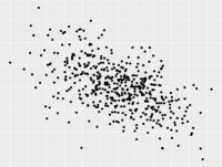
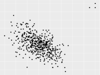
We will illustrate the robustness issue using a simple example. In Figure 1a we see 500 observations that have been simulated from the bivariate Gaussian distribution having correlation . The sample value for Pearson’s is . If we add just three outliers to the data, however, as shown in Figure 1b, the sample correlation changes to . The sample versions of Spearman’s for the simulated data in Figures 1a and 1b are on the other hand very similar: and , and the corresponding values for the estimated Kendall’s are and .
2.3 The nonlinearity issue
This is probably the most serious issue with Pearson’s , and it is an issue also for the rank based correlations of Spearman and Kendall. All of these (and similar measures), are designed to detect rather specific types of statistical dependencies, namely those for which large values of tend to be associated with large values of , and small values of with small values of (positive dependence), or the opposite case of negative dependence in which large values of one variable tend to be associated with small values of the other variable. It is easy to find examples where this is not the case, but where nevertheless there is strong dependence. A standard introductory text book example is the case where
| (6) |
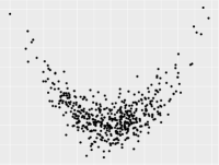
Here, is uniquely determined once is given; i.e., basically the strongest form of dependence one can have. If , however, it is trivial to show that , and moreover that and will also fail spectacularly. A version of this situation is illustrated in Figure 1c, where we have generated 500 observations of the standard normally distributed independent variables and , and calculated as . Still, . The sample values for Pearson’s , Spearman’s and Kendall’s are , and respectively, and none of them are significantly different from zero.
Essentially the same problem will occur if and , where and are independent of each other and independent of . It is trivial to show that if , whereas and are clearly dependent. This example typifies the kind of dependence one has in ARCH/GARCH time series models: If is a time series of zero-mean iid variables and if the time series is independent of , and and are given by the recursive relationship
| (7) |
where the stochastic process is the so-called volatility process, then the resulting model is a GARCH(1,1) model. Further, , and and are non-negative constants satisfying . This model can be extended in many ways and the ARCH/GARCH models are extremely important in finance. A recent book is Francq and Zakoian (2011). The work on these kind of models was initiated by Engle (1982), and he was awarded the Nobel prize for his work. The point as far as Pearson’s is concerned, is that and are uncorrelated for , but they are in fact strongly dependent through the volatility process , which can be taken to measure financial risk. This is probably the best known and most important model class where the dependence structure of the process is not at all revealed by the autocorreletion function. The variables are uncorrelated, but contain a dependence structure that is very important from an economic point of view.
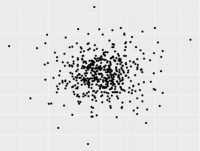
In Figure 1d we see some simulated data from a GARCH(1,1)-model with iid , , and , with on the horizontal axis, and on the vertical axis. In this particular case, , despite the strong serial dependence that is seen to exist directly from equation (7).
The nonlinearity issue will be analysed very extensively and quite systematically in the following sections, but there have also been various more ad hoc solutions to this problem. We will just mention briefly two of them here. Slightly more details are given in the survey paper Tjøstheim (1996), and much more details in the literature cited there.
-
(a)
Higher moments: An «obvious» ad hoc solution in the nonlinear GARCH case is to compute the product moment correlation on squares instead of themselves. It is easily seen that the squares are autocorrelated. This is the idea behind the McLeod and Li (1983) test. It requires the existence of 4th moments, though, which will not always be fulfilled for models of financial time series that typically have heavy tails, see e.g. Teräsvirta et al. (2010, Ch. 8).
-
(b)
Frequency based tests: These are also based on higher product moments, but in this instance one takes the Fourier transform of these to obtain the so-called bi-spectrum and tri-spectrum, on which in turn independence tests can be based (Subba Rao and Gabr 1980; Hinich 1982).
In the following sections we will look at ways of detecting nonlinear and non-Gaussian structures by going beyond Pearson’s .
3 Beyond Pearson’s : The copula
For two variables one may ask, why not just take the joint density function or the cumulative distribution function as a descriptor of the joint dependence? The answer is quite obvious. If a parametric density model is considered, it is usually quite difficult to give an interpretation of the parameters in terms of the strength of the dependence. An exception is the multivariate normal distribution of course, but even for elliptical distributions the «correlation» parameter is not, as we have seen, necessarily a good measure of dependence. If one looks at nonparametric estimates for multivariate density functions, to a certain degree one may get an informal indication of strength of dependence in certain regions from a display of the density, but the problems increase quickly with dimension due both to difficulties of producing a graphical display and to the lack of precision of the estimates due to the curse of dimensionality.
Another problem in analyzing a joint density function is that it may be difficult to disentangle effects due to the shape of marginal distributions and effects due to dependence among the variables involved. This last problem is resolved by the copula construction. Sklar’s (1959) theorem states that a multivariate cumulative distribution function with marginals , can be decomposed as
| (8) |
where is a distribution function over the unit cube . Klaassen and Wellner (1997) point out that Hoeffding (1940) had the basic idea of summarizing the dependence properties of a multivariate distribution by its associated copula, but he chose to define the corresponding function on the interval instead of on the interval . In the continuous case, is a function of uniform variables , using the well-known fact that for a continuous random variable , is uniform on [0,1]. Further, in the continuous case is uniquely determined by Sklar’s (1959) theorem.
The theorem continues to hold for discrete variables under certain weak regularity conditions securing uniqueness. We refer to Nelsen (1999) and Joe (2014) for extensive treatments of the copula. Joe (2014), in particular, contains a large section on copulas in the discrete case. See also Genest and Nešlehová (2007). For simplicity and in keeping with the assumptions in the rest of this paper we will mostly limit ourselves to the continuous case.
The decomposition (8) very effectively disentangle the distributional properties of a multivariate distribution into a dependence part measured by the copula C and a marginal part described by the univariate marginals. Note that is invariant with respect to one-to-one transformations of the marginal variables . In this respect it is analogous to the invariance of the Kendall and Spearman rank based correlation coefficients.
A representation in terms of uniform variables can be said to be in accord with a statistical principle that complicated models should preferably be represented in terms of the most simple variables possible, in this case uniform random variables. A possible disadvantage of the multivariate uniform distribution is that tail behavior of distributions may be difficult to discern on the uniform scale, as it may result in singular type behavior in the corners of the uniform distribution with accumulations of points there in a scatter diagram on or . It is therefore sometimes an advantage to change the scale to a standard normal scale, where the uniform scores are replaced by standard normal scores with being the cumulative distribution of the standard normal distribution. This leads to a more clear representation of tail properties. This scale is sometimes used in copula theory (see e.g. Joe (2014)), and we have used it systematically in our work on local Gaussian approximation described in Section 6.
The decomposition in (8) is very useful in that it leads to
large classes of models that can be specified by defining the marginals
and the copula function separately. It has great flexibility in that
very different models can be chosen for the marginal distribution, and
there is a large catalog of possible parametric models available for the
copula function ; it can also be estimated nonparametrically. The
simplest one is the Gaussian copula. It is constructed from a
multivariate Gaussian distribution with correlation
matrix . It is defined by
| (9) |
such that are standard normal variables for . It should be carefully noted that if one uses (9) in model building, one is still allowed to put in a marginal cumulative distribution functions of one’s own choice, resulting in a joint distribution that is not Gaussian. A multivariate Gaussian distribution with correlation matrix is obtained if the marginals are univariate Gaussians. If the marginals are not Gaussians the correlation matrix in the distribution obtained by (8) will not in general be . Klaassen and Wellner (1997) present an interesting optimality property of the normal scores rank correlation coefficient, the van der Waerden correlation, as an estimate of .
A similar construction taking as its departure the multivariate -distribution can be used to obtain a -copula.
A general family of copulas is the family of Archimedean copulas. It is useful because it can be defined in an arbitrary dimension with only one parameter belonging to some parameter space . A copula is called Archimedean if it has the representation
| (10) |
where is a continuous, strictly decreasing and convex function such that . Moreover, is a parameter within some parameter space . The function is called the generator function and is the pseudo inverse of . We refer to Joe (2014) and Nelsen (1999) for more details and added regularity conditions. In practice, copulas have been mostly used in the bivariate situation, in which case there are many special cases of the Archimedian copula (10), such as the Clayton, Gumbel and Frank copulas. In particular the Clayton copula has been important in economics and finance. It is defined by
| (11) |
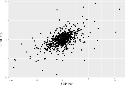
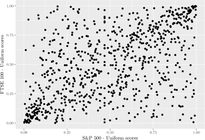
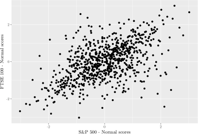
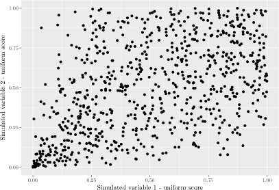
We will throughout this paper illustrate several points using a bivariate data set on some financial returns. We use daily international equity price index data for the United States (i.e. the S&P 500) and the United Kingdom (i.e. the FTSE 100). The data are obtained from Datastream (2018), and the returns are defined as
where is the price index at time . The observation span covers the period from January 1st 2007 through December 31st 2009, in total 784 observations. In Figure 2, four scatterplots are presented.
Figure 2a displays a scatterplot of the observed log-returns, with S&P 500 on the horizontal axis, and the FTSE 100 on the vertical axis. Figure 2b displays the uniform scores of the same data, and we see indications of a singular behavior of the copula density in the lower left and upper right corners of the unit square. In Figure 2c the observations have been transformed to normal scores, which more clearly reveals the tail properties of the underlying distribution. Finally, Figure 2d shows the scatter plot of 784 simulated pairs of variables, on uniform scale, from a Clayton copula fitted to the return data. This plot partially resembles Figure 2b, in particular in the lower left corner. However, there are some differences in the upper right corner. We will look into this discrepancy in Section 6.
In Figure 2a, and perhaps more clearly in Figure 2c, we see that there seems to be stronger dependence between the variables when the market is going either up or down, which is very sensible from an economic point of view, but it is not easy to give an interpretation of the parameter of the Clayton copula in terms of such type of dependence. In fact, in this particular case, . The difficulty of giving a clear and concrete interpretation of copula parameters in terms of measuring strength of dependence can be stated as a potential issue of the copula representation. In this respect it is very different from the Pearson’s . We will return to this point in much detail in Section 6, where we define a local correlation.
Another issue of the original copula approach has been the lack of good practical models as the dimension increases, as it would for example in a portfolio problem in finance. This has recently been sought solved by the so-called pair copula construction. To simplify, in a trivariate density , by conditioning this can be written , and a bivariate copula construction, e.g. a Clayton copula, can be applied to the conditional density with fixed. This conditioning can be extended to higher dimensions under a few simplifying assumptions, resulting in a so-called vine copula, of which there are several types. The procedure is well described by Aas et al. (2009), and has found a number of applications. The Clayton canonical vine copula, for instance, allows for the occurrence of very strongly correlated downside events and has been successfully applied in portfolio choice and risk management operations. The model is able to reduce the effects of extreme downside correlations and produces improved statistical and economical performance compared to elliptical type copulas such as the Gaussian copula (9) and the -copula, see Low et al. (2013).
Other models developed for risk management applications are so-called panic copulas to analyze the effect of panic regimes in the portfolio profit and loss distribution, see e.g Meucci (2011). A panic reaction is taken to mean that a number of investors react in the same way, such that the statistical dependence becomes very strong between financial returns from various financial objects, in this way rendering the risk spreading of the portfolio illusory. We will return to this situation in Section 6 where among other things we can show that in a panic situation the local correlation increases and approaches one as a function of a copula parameter. The copula has also been used directly for independence testing; see e.g. Genest and Rémillard (2004) and Mangold (2017).
Most of the copula theory and also most of the applications are to variables that are assumed to be iid, but there is also a growing literature on stochastic processes such as Markov chains. The existence of both auto dependence and cross dependence in a multivariate stochastic process is quite challenging. Some of the mathematical difficulties in the Markov chain case is clearly displayed in the paper Darsow, Nguyen, and Olsen (1992). They used the ordinary copula, but it is not obvious how the theory of Markov processes can be helped by the concept of a copula. That work was limited to first order Markov chain. The pair copula has also been introduced in a Markov theory framework, and then in higher-order Markov processes, by Ibragimov (2009). Again, so far, the impact on Markov theory has not been overwhelming. This may partly be due to complicated technical conditions.
Two other papers using copulas (and pair copulas) in serial dependence are Beare (2010) and Smith et al. (2010). When it comes to parametric time series analysis, especially for multivariate time series, it has been easier to implement the copula concept as developed for iid variables. This is well documented in the survey paper by Patton (2012). The reason is that the auto dependence can first be filtered out by a marginal fit to each component series, and the copula could then be applied to the residuals which may be assumed to be iid or at least can be replaced by an iid vector process asymptotically. More precisely in the framework of Patton and others,
| (12) |
where in the bivariate case primarily considered by Patton,
Here can be taken as the -algebra generated by for . and is a stochastic vector variable, e.g. higher lags of measurable with respect to . The estimation can be done in two steps, cf. also Chen and Fan (2006). First the parameters of the marginal processes are estimated. Then a copula modeling stage is applied to the estimated residuals
In this context both parametric and nonparametric (resulting in a semiparametric model) models have been considered for the residual distribution . In the parametric case, time dependence can be allowed for , whereas in the nonparametric case there is no dependence of permitted in . Much more details and references are provided in Patton (2012). The modeling in (12) is restricted to the bivariate case. Modeling of both cross and auto dependence, including use of vine copulas, in a multivariate time series or Markov process is given in Smith (2015). Time dependent risk is treated using a dynamic copula model by Oh and Patton (2018).
4 Beyond Pearson’s : Global dependence functionals and tests of independence
Studies of statistical dependence may be said to center mainly around two problems: (i) definition and estimation of measures of dependence and (ii) tests of independence. Of course these two themes are closely related. Measures of association such as the Pearson’s can also be used in tests of independence, or more precisely: tests of uncorrelatedness. On the other hand, test functionals for tests of independence can also in many, but not all, cases be used as a measures of dependence. A disadvantage with measures derived from tests is that they are virtually always based on a distance function and therefore non-negative. This means that they cannot distinguish between negative and positive dependence, whatever this may mean in the general nonlinear case. We will return to this later in the paper.
Most of the test functionals are based on the definition of independence in terms of cumulative distribution functions or in terms of density functions. Consider stochastic variables . These variables are independent if and only if their joint cumulative distribution function is the product of the marginal distribution functions: , and the same is true for all subsets of variables of . If the variables are continuous, this identity can be phrased in terms of the corresponding density functions instead. A typical test functional is then designed to measure the distance between the estimated joint distributions/densities and the product of the estimated marginals. This is not so easily done for parametric densities, since the dependence on parameters in the test functional may be very complex, and tests of independence may be more sensibly stated in terms of the parameters themselves, as is certainly the case for the Gaussian distribution. Therefore one would usually estimate the involved distributions nonparametrically, which, for joint distributions, may be problematic for moderate and large ’s due to the curse of dimensionality. We will treat these problems in some detail in Sections 4.2-4.5.
Before starting on the description of the various dependence measures, let us remark that Rényi (1959) proposed that a measure of dependence between two stochastic variables and , , should ideally have the following 7 properties:
-
(i)
is defined for any neither of which is constant with probability 1.
-
(ii)
.
-
(iii)
.
-
(iv)
if and only if and are independent.
-
(v)
if either or , where and are measurable functions.
-
(vi)
If the Borel-measurable functions and map the real axis in a one-to-one way to itself, then .
-
(vii)
If the joint distribution of and is normal, then , where is Pearson’s .
The product moment correlation satisfies only (i), (ii) and (vii).
One can argue that the rules i) - vii) do not take into account the difference between positive and negative dependence; it only looks at the strength of the measured dependence. If this wider point of view were to be taken into account, (iii) could be changed into (iii’) : , (v) into (v’): or if there is a deterministic relationship between and . Finally, (vii) should be changed into (vii’) requiring . Moreover, some will argue that property (vi) may be too strong to require. It means that the strength of dependence is essentially independent of the marginals as for the copula case.
We will discuss these properties as we proceed in the paper. Before we begin surveying the test functionals as announced above, we start with the maximal correlation which, it will be seen, is intertwined with at least one of the test functionals to be presented in the sequel.
4.1 Maximal correlation
The maximal correlation is based on the Pearson . It is constructed to avoid the problem demonstrated in Section 2.3 that Pearson’s can easily be zero even if there is strong dependence.
It seems that the maximal correlation was first introduced by Gebelein (1941). He introduced it as
where is the Pearson’s . Here the supremum is taken over all Borel-measurable functions with finite and positive variance for and . The measure gets rid of the nonlinearity issue of . It is not difficult to check that if and only if and are independent. On the other hand cannot distinguish between negative and positive dependence, and it is in general difficult to compute.
The maximal correlation cannot be evaluated explicitly except in special cases, not the least because there does not always exist functions and such that . If this equality holds for some and , it is said that the maximal correlation between and is attained. Rényi (1959) gave a characterization of attainability.
Czáki and Fischer (1963) studied mathematical properties of the maximal correlation and computed it for a number of examples. Abrahams and Thomas (1980) considered maximal correlation in the context of stochastic processes. A multivariate version of maximal correlation was proposed in Koyak (1987). In a rather influential paper, at least at the time, Breiman and Friedman (1985) presented the ACE (alternating conditional expectation) algorithm for estimating the optimal functions and in the definition of the maximal correlation. They applied it both to correlation and regression. Some curious aspects of the ACE algorithm is highlighted in Hastie and Tibshirani (1990, 84–86).
Two more recent publications are Huang (2010), where the maximal correlation is used to test for conditional independence, and Yenigün, Székely, and Rizzo (2011), where it is used to test for independence in contingency tables. The latter paper introduces a new example where can be explicitly computed. See also Yenigün and Rizzo (2014).
4.2 Measures and tests based on the distribution function
We start with, and in fact put the main emphasis on, the bivariate case. Let and be stochastic variables with cumulative distribution functions and . The problem of measuring the dependence between and can then be formulated as a problem of measuring the distance between the joint cumulative distribution function of and the distribution function formed by taking the product of the marginals. Let be a candidate for such a distance functional. It will be assumed that is a metric, and it is natural to require, Skaug and Tjøstheim (1996), that
| (13) |
Clearly, such a measure is capable only of measuring the strength of dependence, not its direction. Corresponding to requirement (vi) in Rényi’s scheme listed in the beginning of this section, one may want to require invariance under transformations, or more precisely
| (14) |
where , and . Here and are increasing functions, and are the marginals and bivariate distribution functions of the random variables and , respectively.
For distance functionals not satisfying equation (14), one can at least obtain scale and location invariance by standardizing such that and , assuming that the second moment exists. In practice, empirical averages and variances must be employed, but asymptotically the difference between using empirical and theoretical quantities is a second order effect. In Skaug and Tjøstheim (1996) and Tjøstheim (1996) such a standardization has been employed for all functionals.
Pearson’s can be expressed as a functional on , and although not generally as a distance functional depending on and . For instance, with and standardized, the Pearson correlation squared can be expressed,
Clearly does not satisfy either of the conditions (13) or (14). Similarly, the square of the population values of the Spearman rank correlation and Kendall’s are obtained by squaring in the formulas (4) and (5). For these measures the requirement (13) is not fulfilled, whereas the invariance property does hold.
A natural estimate of a distance functional is obtained by setting
where may be taken to be the empirical distribution functions given by
and
or a normalized version with replaced by for given observations . Similarly, for a stationary time series at lag ,
Conventional distance measures between two distribution functions and are the Kolmogorov-Smirnov distance
and the Cramér-von Mises type distance of a distribution from a distribution
Here satisfies (13) and (14), whereas satisfies (13) but not (14).
Most of the work pertaining to measuring dependence and testing of independence has been done in terms of the Cramér-von Mises distance. This work started already by Hoeffding (1948) who looked at iid pairs , and studied finite sample distributions in some special cases. With considerable justification it has been named the Hoeffding-functional by some. This work was continued by Blum, Kiefer, and Rosenblatt (1961) who provided an asymptotic theory, still for the iid case. It was extended to the time series case with a resulting test of serial independence in Skaug and Tjøstheim (1993a). A recent paper using a copula framework is Kojadinovic and Holmes (2009). We will briefly review the time series case because it illustrates some of the problems, and because some of the same essential ideas as for the Hoeffding-functional have been used in more recent work on the distance covariance, which we treat in Section 4.3. Since does not depend on for a stationary time series, we simply write in the following.
In the time series case the Cramér-von Mises distance at lag is given by
where and are the joint and marginal distributions of and , respectively. Replacing theoretical distributions by empirical ones leads to the estimate
| (15) |
Assuming to be ergodic, we have that almost surely as .
To construct a test of serial independence we need the distribution of under the assumption of the null hypothesis of being iid. Let . Then it is possible to represent as
where is a von Mises U-statistic in the technical sense of Denker and Keller (1983) with a degenerate symmetric kernel function. Using asymptotic theory, Carlstein (1988), Denker and Keller (1983) and Skaug (1993), of this statistic or the related U-statistic one has (Skaug and Tjøstheim 1993a, Theorem 2) the convergence in distribution
| (16) |
where is an independent identically distributed sequence of variables, and where the are the eigenvalues of the eigenvalue problem
with
If the distribution of each is continuous, then is distribution free, i.e., its distribution does not depend on . Then all calculations can be carried out with being the uniform distribution, in which case and , and the distribution of the right hand side of (16) can be tabulated by truncating it for a large value of the summation index. Similar distribution results will be seen to hold for test functionals in Sections 4.3 and 4.4.
A test of the null hypothesis of independence, or rather pairwise independence at lag , can now be constructed. It is then reasonable to reject if large values of is observed. Thus a test of level is:
where is the upper -point in the null distribution of . Since the exact distribution of is unknown, we can use the asymptotic approximation furnished by retaining a finite number of terms in (16). For and small this works well. However, as increases, in general (Skaug and Tjøstheim 1993a) the level is severely overestimated. The results of Skaug and Tjøstheim (1993a) have since been very considerably extended and improved by Hong (1998).
Under the hypothesis of being iid the bootstrap is a natural tool to use for constructing the null distribution and critical values. For moderate and large ’s the bootstrapping yields a substantially better approximation to the level.
Under the alternative hypothesis that and are dependent, the test statistic will in general be asymptotically normal with a different rate from that of (16), but the power function will be complicated; see e.g. Hong (2000).
To extend the scope to testing of serial dependence among , or alternatively between a set of several random variables for which there are iid observations of the set, one might use a functional
| (17) |
The asymptotic theory under the null hypothesis of independence for such a test has been examined by Delgado (1996) using empirical process theory, but due to the curse of dimensionality, problems in practice might be expected for moderately large ’s. As an alternative Skaug and Tjøstheim (1993a) used a “Box-Pierce-Ljung” analogy, testing for pairwise independence in all of the pairs using the statistic
| (18) |
The asymptotic theory of such a test is given in Skaug (1993). Hong (1998) noted that
| (19) |
has better size properties for large .
There have been several contributions to the limit theory of statistics such as (15) and (17) using empirical process theory. Delgado did that based on developments in Blum, Kiefer, and Rosenblatt (1961), but the limiting Gaussian process is complicated with a complex covariance matrix which makes it difficult to tabulate critical values. Ghoudi, Kulperger, and Rémillard (2001) based their work on the so-called Möbius transformation promoted by Deheuvels (1981a; 1981b) in his papers on independence testing. This transformation takes explicitly into account the joint distribution function of all subsets of mentioned in the second paragraph of Section 3. To explain the Möbius transformation, let , be random variables. For let denote the marginal cumulative distribution function of and let be the corresponding joint cumulative distribution function. Consider a subset , and for any , define
where is the number of elements in a set , , where by convention , and where is the vector whose th component is defined by if , and otherwise. Then one can state the following criterion of independence: are independent if and only if for any . This is shown in e.g. Ghoudi, Kulperger, and Rémillard (2001). In that paper it is also shown how this transformation leads to a Gaussian empirical process limit with a relatively simple covariance function, making it easier to tabulate critical values. The authors manage to do this both for the Cramér-von Mises statistic and the Kolmogorov-Smirnov statistic, and they consider three cases: iid vector samples, time series samples and residuals in time series models. See also Beran, Bilodeau, and Lafaye de Micheaux (2007).
Genest and Rémillard (2004) use the Möbius transformation in testing of independence in a copula framework, and Ghoudi and Rémillard (2018) use it to obtain tests for independence of residuals in a parametric model
where the iid innovations have mean 0 and variance 1.
As an alternative to testing uncorrelatedness in time series using the Pearson at accumulated lags as in the Box-Ljung-Pierce statistic, one could test for a constant spectral density. Quite general specification tests in terms of the spectral density has been considered by Anderson (1993), who looked at tests of constant by using both the Cramér-von Mises and the Kolmogorov-Smirnov criteria. Hong (2000) introduced a spectral counterpart for the independence tests based on the marginal distribution function for a time series and the lag distribution function introduced earlier in this section. This was achieved by replacing the ordinary autocorrelation function by the dependence measure
and then taking Fourier transforms, which leads to
| (20) |
where . It is shown in Hong (2000) how this can be used to construct a test of independence that has power in cases where the tests based on the ordinary spectrum has not. However, as explained in a note in that paper, weak power can be expected for this test against ARCH/GARCH type dependence.
Instead of stating independence in terms of cumulative distribution functions this can alternatively be expressed in terms of the characteristic function. Székely, Rizzo, and Bakirov (2007) and Székely and Rizzo (2009), as will be seen in Section 4.3, make systematic use of this in their introduction of the distance covariance test. Two random variables and are independent if and only if the characteristic functions satisfy
where
This was exploited by Csörgö (1985) and Pinkse (1998) to construct tests for independence based on the characteristic function in the iid and time series case, respectively. Further work on testing of conditional independence was done by Su and White (2007). See also Fan et al. (2017). Hong (1999) put this into a much more general context by replacing in (20) by
By taking Fourier transform of this quantity one obtains
| (21) |
Hong (1999) called (21) the generalized spectral density function. Here can be estimated by
where is a kernel weight function, is a bandwidth or lag order, and
with
Under the null hypothesis of serial independence becomes a constant function of frequency :
with , where . In order to test for independence one can compare and using e.g. an -functional. More work related to this has been done by Hong and Lee (2003) and Escanciano and Velasco (2006).
4.3 Distance covariance
We have seen that there are at least two ways of constructing functionals that are consistent against all forms of dependence, namely those based on the empirical distribution function initiated by Hoeffding (1948) and briefly reviewed above, and those based on the characteristic function represented by Csörgö (1985) in the iid case and Pinkse (1998) in the serial dependence case, and continued in Hong (1999; 2000) in a time series spectrum approach. Se also Fan et al. (2017). Both Pinkse and Hong use a kernel type weight function in their functionals. Thus, Pinkse uses a weight function in the functional
where for a pair of two random variables
Let . Pinkse in his simulation experiments chose the weight functions and .
The authors of two remarkable papers, Székely, Rizzo, and Bakirov (2007) and Székely and Rizzo (2009), take up the characteristic function test statistic again in the non-time series case. But what distinguishes these from earlier papers is an especially judicious choice of weight function reducing the empirical characteristic function functional to empirical moments of differences between the variables, or distances in the vector case, this leading to covariance of distances. Some of these ideas go back to what the authors term an “energy statistic”; see Székely (2002), Székely and Rizzo (2013) and also Székely and Rizzo (2012). It has been extended to time series and multiple dependencies by Davis et al. (2018), Fokianos and Pitsillou (2017), Zhou (2012), and Dueck et al. (2014), Dueck, Edelman, and Richards (2015) and Yao, Zhang, and Shao (2018). In the locally stationary time series case there is even a theory, see Jentsch et al. (2018). The distance covariance, dcov, seems to work well in a number of situations, and it has been used as a yardstick by several authors writing on dependence and tests of independence. In particular it has been used as a measure of comparison in the work on local Gaussian correlation to be detailed in Section 6. There are also points of contacts, as will be seen in Section 4.4, with the HSIC measure of dependence popular in the machine learning community.
The central ideas and derivations are more or less all present in Székely, Rizzo, and Bakirov (2007). The framework is that of pairs of iid vector variables in and , respectively, and the task is to construct a test functional for independence between and . Let , and be the characteristic functions involved, where is the inner product in and , respectively. The starting point is again the weighted characteristic functional
| (22) |
where is a weight function to be chosen, Note that it is easy to choose so that if and only if and are independent. Similarly, one defines
| (23) |
and . The distance correlation, dcor, is next defined by, assuming ,
These quantities can be estimated by the empirical counterparts given observations of the vector pair with
| (24) |
where, for a set of observations the empirical characteristic functions are given by
and
It turns out that it is easier to handle the weight function in the framework of the empirical characteristic functions. It will be seen below that
| (25) |
is a good choice. Here is the Euclidean norm in and similarly for . Moreover, the normalizing constants are given by , . For it to make sense to introduce the weight function on the empirical characteristic function one must show that the empirical functionals converges to the theoretical functionals for this weight function. This is not trivial because of the singularity at for given by (25). A detailed argument is given in the proof of Theorem 2 in Székely, Rizzo, and Bakirov (2007).
The advantage of introducing the weight function for the empirical characteristic functions is that one can compute the squares in (24) and then interchange summation and integration. The resulting integrals can be computed using trigonometric identities, in particular the odd symmetry of products of cosines and sines which makes corresponding integrals disappear. The details are given in the proof of Theorem 1 in Székely, Rizzo, and Bakirov (2007) and in Lemma 1 of the Appendix of Szekely and Rizzo (2005) who in turn refer to Prudnikov, Brychkov, and Marichev (1986) for the fundamental lemma
for with
| (26) |
and where the weight function considered above corresponds to and or in (25). The general -case corresponds to a weight function
With the simplification all of this implies that as defined in (24), can be computed as
where
| (27) |
which explains the appellation distance covariance. In fact, it is possible to further simplify this by introducing
for . Similarly, one can define and and
and
and similarly for . From this one can easily compute . The computations are available in an R-package: Rizzo and Szekely (2018).
As is the case of the empirical joint distribution functional it can be expected that the curse of dimensionality will influence the result for large and moderate values of and . Obviously, in the time series case, it is possible to base oneself on pairwise distances as in (18) or (19), which has been done in Yao, Zhang, and Shao (2018).
Letting , it is not difficult to prove that an alternative expression for is given by (assuming and )
| (28) |
where , are iid. This expression will be useful later in Section 4.4 in a comparison with the HSIC statistic. Properly scaled has a limiting behavior under independence somewhat similar to that of (16) in Section 4.2. Namely, under the condition of existence of first moment, , converges in distribution to a quadratic form
where are independent standard normal variables, are non-negative constants that depend on the distribution of . One can also obtain an empirical process limit theorem, Theorem 5 of Székely, Rizzo, and Bakirov (2007). In the R-package, as for the case of the empirical distribution function, it has been found advantageous to rely on re-sampling via permutations. This is quite fast since the algebraic formulas (27) are especially amenable to permutations. Both Székely, Rizzo, and Bakirov (2007) and Székely and Rizzo (2009) in their experiments only treat the case of in (26).
Turning to the properties (i) - (vii) of Rényi (1959) listed in the beginning of this section, it is clear that (i) - (iv) are satisfied by . Moreover, according to Székely, Rizzo, and Bakirov (2007), if , then there exists a vector , a non-zero real number and an orthogonal matrix such that , which is not quite the same as Rényi’s requirement (v). Also, the general invariance in his property (vi) does not seem to hold. The final criterion (vii) of Rényi is that the dependent measure should reduce to the absolute value of Pearson’s in the bivariate normal case. This is not quite the case for the dcov, but it comes close, as is seen from Theorem 6 of Székely and Rizzo (2009). In fact, if is bivariate normal with and and with correlation , then and
4.4 The HSIC measure of dependence
Recall the definition and formula for the maximal correlation. This, as stated in Section 4.1 gives rise to a statistic , where if and only if and are independent. But it is difficult to compute since it requires the supremum of the correlation taken over Borel-measurable and . In the framework of reproducing kernel Hilbert spaces (RKHS) it is possible to pose this problem, or an analogous one, much more generally, and one can compute an analogue of quite easily. This is the so-called HSIC (Hilbert-Schmidt Independence Criterion).
Reproducing kernel Hilbert spaces are very important tools in mathematics as well as in statistics. A general reference to applications in statistics is Berlinet and Thomas-Agnan (2004). In the last decade or so there has also been a number of uses of RKHS in dependence modeling. These have often been published in the machine learning literature. See e.g Gretton, Herbrich, et al. (2005), Gretton and Györfi (2010), Gretton and Györfi (2012) and Sejdinovic et al. (2013).
We have found the quite early paper by Gretton, Bousquet, et al. (2005) useful both for a glimpse of the general theory and for the HSIC criterion in particular.
A reproducing kernel Hilbert space is a separable Hilbert space of functions on a set , such that the evaluation functional is a continuous linear functional on for every . Then, from the Riesz representation theorem, Muscat (2014), chapter 10, there exists an element such that , where is the inner product in . Applying this to and another point we have . The function from to is the kernel of the RKHS . It is symmetric and positive definite because of the symmetry and positive definiteness of the inner product in . We use the notation for the kernel.
The next step is to introduce another set with a corresponding RKHS and to introduce a probability structure and probability measures , and on , and , respectively. With these probability measures and function spaces and one can introduce correlation of functions of stochastic variables on , and . This is an analogy of the functions used in the definition of the maximal correlation. In RKHS setting the covariance (or cross covariance) is an operator on the function space . Note also that this has a clear analogy in functional statistics, see e.g. Ferraty and Vieu (2006).
It is time to introduce the Hilbert-Schmidt operator: A linear operator is called a Hilbert-Schmidt operator if its Hilbert-Schmidt (HS) norm
where and are orthonormal bases of and , respectively. The HS-norm generalizes the Froebenius norm for a matrix . Finally, we need to define the tensor product in this context: If and , then the tensor product operator is defined by
Moreover, by using the definition of the HS norm it is not difficult to show that
We can now introduce an expectation and a covariance on these function spaces. Again, the analogy with corresponding quantities in functional statistics will be clear. We assume that and are furnished with probability measures , and with and being -algebras of sets on and . The expectations and are defined by, and are stochastic variables in and , respectively,
and
where and are well-defined as elements in and because of the Riesz representation theorem. The norm is obtained by
where as before and are independent but have the same distribution , and where is defined in the same way. With given , we can now define the cross covariance operator as
Now, take to be identified with defined above as a result of the Riesz representation theorem, and defined in exactly the same way. The Hilbert-Schmidt Information Criterion (HSIC) is then defined as the squared HS norm of the associated cross-covariance operator
Let and be kernel functions on and . Then (Gretton, Bousquet, et al. 2005, Lemma 1), the HSIC criterion can be written in terms of these kernels as
| (29) |
Existence is guaranteed if the kernels are bounded. The similarity in structure to (28) for the distance covariance should be noted (partly due to the identity but going deeper as will be seen below when HSIC is compared to dcov). Note that the kernel functions depend on the way the spaces and and their inner products are defined. In fact it follows from a famous result by Moore-Aronszajn, see Aronszajn (1950), that if is a symmetric, positive definite kernel on a set , then there is a unique Hilbert space of functions on for which is a reproducing kernel. Hence as will be seen next, in practice when applying the HSIC criterion, the user has to choose a kernel.
With some restrictions the HSIC measure is a proper measure of dependence in the sense of the Rényi (1959) criterion (iv): From Theorem 4 of Gretton, Bousquet, et al. (2005) one has that if the kernels and are universal (universal kernel is a mild continuity requirement on the kernel) on compact domains and , then if and only if and are independent. The compactness assumption results from the application of an equality for bounded random variables taken from Hoeffding (1963), that is being used actively in the proof.
A big asset of the HSIC measure it that its empirical version is easily computable. In fact if we have independent observations and independent observations , then
| (30) |
where tr is the trace operator and the matrices are defined by
where is the Kronecker delta. It is shown in Gretton, Bousquet, et al. (2005) that this estimator converges towards . The convergence rate is . There is also a limit theorem for the asymptotic distribution, which under the null hypothesis of independence and scaled with converges in distribution to the random variable , where the are independent standard normal variables, and and are eigenvalues of integral operators associated with centralized kernels derived from and and integrating using the probability measures and , respectively. Again, this should be compared to the limiting variable for the statistic in the Cramér- von Mises functional (16). Critical values can be obtained for , but as a rule one seems to rely more on resampling as is the case for most independence test functionals.
It is seen from (30) that computation of the empirical HSIC criterion requires the evaluation of and . Then appropriate kernels have to be chosen. Two commonly used kernels are the Gaussian kernel given by
and the Laplace kernel
Pfister and Peters (2017) describe a recent R-package involving HSIC. Gretton, Bousquet, et al. (2005) use these kernels in comparing the HSIC test with several other tests, including the dcov test in, among other cases, an independent component setting. Both of these tests do well, and one of these tests does not decisively out-compete the other one. This is perhaps not so unexpected because there is a strong relationship between these two tests. This is demonstrated by Sejdinovic et al. (2013). They look at both the dcov test and the HSIC test in a generalized setting of semimetric spaces, i.e with kernels and distances defined on such spaces and . For a given distance function they introduce a distance-induced kernel, and under certain regularity conditions they establish a relationship between these two quantities. There is a related paper by Lyons (2013) which obtains similar results but not in an explicit RKHS context, in fact in a general dcov context.
Let and be distance measures on the semi-metric spaces and , respectively. Then a generalized dcov distance functional can be defined as, compare again to (28),
This distance covariance in metric spaces characterizes independence, that is, if and only if and are independent, and if the metrics and satisfy an additional property, termed strong negative type. See Sejdinovic et al. (2013) for more details. An asset of the RKHS formulation is that it is very general. As was seen from the introduction of HSIC above, the sets and can have a metric space structure, and probability measures , and can still be introduced, and the definition of HSIC given in the beginning of this section and the accompanying decomposition (29) still make sense in this generalized framework. It can then be shown that, Theorem 24 in Sejdinovic et al. (2013), one has the following equivalence: Let and be any two kernels on and that generate and , respectively, and let , then . Among the regularity conditions required for this result is the assumption of “negative type”, which is satisfied in standard Euclidean spaces.
However, it is not possible to find a direct RKHS representation of the characteristic function representation (23) of .
Lately there have been other extensions of both the dcov and HSIC to conditional dependence, partial distance and to time series. A few references are Szekely and Rizzo (2014), Chwialkowski and Gretton (2014), Zhang et al. (2012) and Pfister et al. (2018). A recent tutorial on RKHS is Gretton (2017).
4.5 Density based tests of independence
Intuitively, one might think that knowing that the density exists should lead to increased power of the independence tests due to more information. This is true, at least for some examples (see e.g. Teräsvirta, Tjøstheim, and Granger (2010), Chapter 7.7). As in the preceding sections one can construct distance functionals between the joint density under dependence and the product density under independence. A number of authors have considered such an approach; both in the iid and time series case, see e.g. Rosenblatt (1975), Robinson (1991), Skaug and Tjøstheim (1993b; 1996), Granger, Maasoumi, and Racine (2004), Hong and White (2005), Su and White (2007) and Berrett and Samworth (2017). For two random variables and having joint density and marginals and the degree of dependence can be measured by , where is now the distance measure between two bivariate density functions. The variables are normalized with and . It is natural to consider the Rényi (1959) requirements again, in particular the requirements (iv) and (vi).
All of the distance functionals considered will be of type
| (31) |
where is a real-valued function such that the integral exists. If is of the form , we have
| (32) |
which by the change of variable formula for integrals is seen to have the Rényi property (vi). Moreover, if and if and only if , then Rényi property (iv) is fulfilled. Several well-known distance measures for density functions are of this type. For instance, letting we obtain the Hellinger distance
between and . The Hellinger distance is a metric and hence satisfies the Rényi property (iv).
Chung et al. (1989) defined the so-called directed divergence of degree , which is also related to the Rényi divergence, Rényi (1961),
| (33) |
It is seen that the Hellinger distance is a special case . Clearly, the measure satisfies (vi), and for , using Hölder’s inequality,
with equality if and only if . Hence, satisfies (iv) for .
The familiar Kullback-Leibler information (entropy) distance is obtained as a limiting case as ,
| (34) |
Since this distance is of type (32), it satisfies (vi), and it can also be shown to satisfy (iv). Going outside the range , for in (33), the test-of-fit distance in Bickel and Rosenblatt (1973) emerges. See also Granger and Lin (1994). A very recent paper linking with other recent approaches to independence testing is Berrett and Samworth (2017).
All of the above measures are trivially extended to two arbitrary multivariate densities. However, estimating such densities in high or moderate dimensions may be difficult due to the curse of dimensionality. A functional built up from pairwise dependencies can be considered instead such as in (18) and (19).
For a given functional depending on two densities and , may be estimated by . There are several ways of estimating the densities, e.g. the kernel density estimator,
for given observations . Here , where is the bandwidth (generally a matrix), is the kernel function, and is the dimension of . The kernel function is usually taken to be a product of one-dimensional kernels; i.e., , where each generally is non-negative and satisfies
Once estimators for , and in the integral expression (31) for have been obtained, the integral can be computed by numerical integration or by empirical averages using the ergodic theorem (or law of large numbers in the iid case). Consequently for a given lag in the time series case,
Here is the joint density of , and is a weight function, e.g., for some chosen constant .
Under regularity conditions (see e.g. Skaug and Tjøstheim (1996)}, consistency and asymptotic normality can be obtained for the estimated test functionals. It should be noted that the leading term in an asymptotic expansion of the standard deviation of for the estimated Kullback-Leibler functional and the estimated Hellinger functional is of order . This is of course the same as for the standard deviation of a parametric estimate in a parametric estimation problem. In that situation the next term of the Edgeworth expansion is of order , and for moderately large values of the first order term will dominate. However, for the functionals considered above, due to the presence of an -dependent bandwidth, the next terms in the Edgeworth expansion are much closer, being of order and , and since typically or , must be very large indeed to have the first term dominate in the asymptotic expansion. As a consequence, first order asymptotics in terms of the normal approximation cannot be expected to work well unless is exceedingly large. Hence, basing a test of independence directly on the asymptotic theory may be hazardous as the real test size will typically deviate substantially from the nominal size. In this sense the situation is quite different from the empirical functionals treated in the previous sections, where there is no bandwidth parameter involved.
All of this suggests the use of the bootstrap or permutations as an alternative for constructing the null distribution. One may anticipate that it picks up higher-order terms of the Edgeworth expansion (Hall 1992, Chapters 3 and 4), although no rigorous analysis to confirm this has been carried out for the functionals discussed here.
The fact that the permutation test yields an exact size, and that resampling tests generally perform much better, underscores a major point. In tests involving a bandwidth it is absolutely essential to use resampling in practice. The asymptotic theory is far too inaccurate except possibly in cases where the sample size is extremely large. In the empirical functional case treated in Sections 4.2 and 4.3, the asymptotic theory is incomparably more accurate, but even in this case the experience so far seems to be that resampling generally does slightly better.
It is quite difficult to undertake local asymptotic power analyses for the functionals based on estimated density functions. For reasons mentioned above, asymptotic studies could be expected to be unreliable unless is very large. It has therefore been found more useful to carry out comparative simulation studies against a wide choice of alternatives using a modest sample size, see e.g. Skaug and Tjøstheim (1993; 1996) and Hong and White (2005). These references also contain applications to real data.
4.6 Test functionals generated by local dependence relationships
If one has bivariate normal data with standard normal marginals and one gets observations scattered in a close to circular region around zero, and most test functionals will easily recognize this as a situation of independence. However, as pointed out by Heller, Heller, and Gorfine (2013), if data are generated along a circle, e.g. for some stochastic noise variable , then and are dependent, but the dcov, and undoubtedly other test functionals, among which -based tests, fail. They give some other examples as well of similar failures for test functionals to detect symmetric geometric patterns. Heller, Heller, and Gorfine (2013) point a way out of this difficulty, namely by looking at dependence locally (along the circle) and then aggregate the dependence by integrating or by other means over the local regions. There are of course several ways of measuring local dependence and we will approach this problem more fundamentally in Section 5.
Before coming to the paper by Heller, Heller, and Gorfine (2013) and papers using similar approaches, partly for historic reasons, we look briefly at the correlation integral and the so-called BDS test named after its originators Brock, Dechert and Scheinkman. This test has a local flavor at its basis, but the philosophy is a bit different from the other tests presented in the current subsection. The BDS test attracted much attention among econometricians in the 1990s, and it has since been improved.
The starting point is the correlation integral introduced in Grassberger and Procaccia (1983) as a means of measuring fractal dimension of deterministic data. It measures serial dependence patterns in the sense that it keeps track of the frequency with which temporal patterns are repeated in a data sequence. Let be a sequence of numbers and let
Then the correlation integral for embedding dimension is given by
Here, for , , where is the indicator function and is a cut off threshold which could be a multiple of the standard deviation in the case of a stationary process. The parameter may also be considered to be a tuning parameter. Let
If is an absolutely regular (Bradley, 1986, p.169) stationary process the above limit exists and is given by
where is the joint cumulative distribution function of . Since
it is easily seen that if consists of iid random variables, then
This theory is the starting point for the BDS test. Under the hypothesis of independence, and excluding the case of uniformly distributed random variables, Broock et al. (1996) have established asymptotic normality of under an appropriate scaling factor . As mentioned, the test has found considerable use among econometricians, but it suffers from some limitations, the arbitrariness of the choice of , the probability of rejecting independence does not always approach 1 as , and finally, and probably most critically, the convergence to the asymptotic normal distribution may be very slow, making bootstrapping a possible alternative. These problems were pointed out by Genest, Ghoudi, and Rémillard (2007) who proposed a rank based extension, where these difficulties are to a large degree eliminated. Because the limiting distribution of the rank-based test statistics is margin-free, their finite-sample p-values can be easily calculated by simulations.
Next, returning to the test of Heller, Heller, and Gorfine (2013), note that if and (in and , say) are continuous and are dependent, then there exists a point in the sample space of , and radii and around and , respectively, such that the joint distribution of is different from the product of the marginals in the neighborhood defined by and . The next step is the introduction of a distance functions in the sample spaces of and , and following Heller, Heller, and Gorfine (2013) we do not distinguish between these distance functions in our notation. Consider the indicator functions and . For a sample one gets pairs of values of zeros and ones from the indicator functions that can be set up in a contingency table structure. Evidence against independence may then be quantified by Pearson’s chi-square test statistic or the likelihood ratio test for contingency tables.
The data is used to guide in the choice of , and . For every sample point , that point is in its turn chosen to be and for every sample point , , it is chosen in turn to define and (thus defining the locality of the test). The remaining observations are then inserted in the indicator functions. For every pair based on this one can construct a classic test statistic for a Pearson chi-square test for a contingency table. To test for independence these quantities are aggregated in a test statistic . Critical values are obtained by resampling. The test, taking local properties into account, works very well for the circle example and several other examples, both similar to the circle example and not. See also Heller et al. (2016).
The next paper in this category, Reshef et al. (2011), is published in Science. The idea behind their MIC (Maximal Information Coefficient) statistic consists in computing the mutual information as defined in (34) locally over a grid in the data set and then take as statistic the maximum value of these local information measures as obtained by maximizing over a suitable choice of grid. The authors compare with several other classifiers on simulated and real data with apparently good results. Some limitations of the method are identified in a later article by Reshef et al. (2013). Another follow-up article is Chen et al. (2016). See also Kinney and Atwal (2014), Reshef et al. (2014) and Murrell, Murrell, and Murrell (2014). There are, however, publications where the results are more mixed. See Simon and Tibshirani (2014) and Gorfine, Heller, and Heller (2012). In particular these two papers give several examples where the MIC is clearly inferior to dcov.
The two final papers in this category are Wang et al. (2015) and Wang et al. (2017). In both papers the authors defines the locality by means of a neighborhood of and then consider suitable -values. Consequently, as remarked by Wang et al. (2015) their test may be best suited to nonlinear regression alternatives of the form . Wang et al. (2015) denote by , observations of the stochastic variables and in the construction of their CANOVA test statistic. They define the within neighborhood sum of squares statistic as
where is an integer constant which is supposed to be chosen by the user. Then defines the -neighborhood structure. The assumption of CANOVA is that dependence should imply that “similar/neighbor -values lead to similar -values”. Thus when and are dependent, small values of are expected. Critical values of is determined by permutations. The test for 4 values of (2, 4, 8, 12) is compared to a number of other tests among them Pearson’s , the Kendall and Spearman correlation coefficients, dcov, MIC, and the Hoeffding-test based on the empirical distribution function. The CANOVA tests does not do particularly well for linear models and it fails for the circle data with weak noise, but its performance on the tested nonlinear examples is very good.
The paper by Wang et al. (2017) follows much of the same pattern and ideas. The -values are first used to construct bagging neighborhoods. And then they get an out-of-bag estimator of , based on the bagging neighborhood structure. The square error is calculated to measure how well is predicted by . Critical values are again obtained by permutations in the resulting statistic. In a comparison with other methods five out of eight examples consist of various sinusoidal function with added noise, where the new test does very well.
5 Beyond Pearson’s : Local dependence
The test functionals treated in Section 4 deal with the the second aspect of modelling dependence stated in the beginning of that section, namely that of testing of independence. These functionals all do so by the computation of one non-negative number, which is derived from local properties in Section 4.6. This number properly scaled may possibly be said to deal with the the first aspect stated, namely that of measuring the strength of dependence. But, as such, it can be faulted in several ways. Unlike the Pearson , these functionals do not distinguish between positive and negative dependence, and it is not local, thus not allowing for stronger dependence in multivariate tails as is felt intuitively is the case for data in finance for example.
In Section 6 the main story will be the treatment of local Gaussian correlation which in a sense returns to the Pearson but a local version of which satisfies many of Rényi (1959)’s requirements. But first, in the present section, we go back to some other attempts to define local dependence, starting with a remarkable paper by Lehmann (1966), who manages to define positive and negative dependence in a quite general nonlinear situation.
5.1 Quadrant dependence
Lehmann’s theory is based on the concept of quadrant dependence. Consider two random variables and with cumulative distribution . Then the pair or its distribution function is said to be positively quadrant dependent if
| (35) |
Similarly, or is said to be negatively quadrant dependent if (35) holds with the central inequality sign reversed.
The connection between quadrant dependence and Pearson’s is secured through a lemma of Hoeffding (1940). The lemma is a general result and resembles the result by Székely (2002) in his treatment of the so-called Cramér functional, a forerunner of the Cramér - von Mises functional. If denotes the joint and and the marginals, then assuming that the necessary moments exist,
It follows immediately from definitions that if is positively quadrant dependent (negatively quadrant dependent), then for the Pearson’s , (). Similarly, it is shown by Lehmann that if is positively quadrant dependent, then Kendall’s , Spearman’s , and the quadrant measure defined by Blomqvist (1950) are all non-negative. The paper by Blomqvist is an even earlier paper where positive and negative dependence were considered in a nonlinear case, and using quadrants centered at the median. An analogous result holds in the negatively quadrant dependent case.
Lehmann (1966) introduces two additional and stronger concepts of dependence. The first is regression dependence. Definition (35) can be written
but following Lehman, it may be felt that the intuitive concept of positive dependence is better represented by the stronger condition
| (36) |
Rather than (36), Lehmann considers the stronger condition
which was discussed earlier by Tukey (1958). The concept of negative regression dependence is defined by an obvious analog.
Finally, Lehmann introduces a stronger type of dependence still, by requiring the conditional density of given to have a monotone likelihood ratio. Assuming the existence of a density , the condition may be written formally as
If the inequality is reversed is said to be negatively likelihood ratio dependent. The bivariate normal distribution is positively or negatively likelihood ratio dependent according to or . We will briefly return to these dependence concepts when we get to the local Gaussian correlation in Section 6.
5.2 Local measures of dependence
As mentioned already, econometricians have long looked for a formal statistical way of describing the shifting region-like dependence structure of financial markets. It is obvious that when the market is going down there is a stronger dependence between financial objects, and very strong in case of a panic. Similar effects, but perhaps not quite so strong, appear when the market is going up. But how should it be quantified and measured? This is important in finance, not the least in portfolio theory, where it is well-known, see e.g. Taleb (2007), that ordinary Gaussian description does not work, and if used, may lead to catastrophic results. Mainly two approaches have been used among econometricians. The first is non-local and consists simply in using copula theory, but it may not always be so easy to implement in a time series and portfolio context. The other approach is local and is to use “conditional correlation” as in Silvapulle and Granger (2001) and Forbes and Rigobon (2002). One then computes an estimate as in (1) of Pearson’s but in various regions of the sample space, e.g. in the tail of two distributions. Let be such a region. A conditional correlation estimate is then given by (we let be the number of observed pairs and , and similarly for ),
However, this estimate suffers from a serious bias, which is obvious by using the ergodic theorem or the law of large numbers, in the sense that for a Gaussian distribution it does not converge to . This is unfortunate because if the data happen to be Gaussian, one would like estimated correlations to be close or identical to in order to approximate the classic Gaussian portfolio theory of Markowitz (1952). This requirement is consistent with Rényi’s property (vii).
The bias is examined in Boyer, Gibson, and Loretan (1999). Consider, as an example, a bivariate Gaussian distribution with correlation . The conditional correlation when one of the variables is large, for example larger than its 75% quantile, , is reduced to 0.27, and as the quantile increases converges to zero. In the finance literature one has tried to correct for this for instance in contagion studies, Forbes and Rigobon (2002). What is wrong here, one may think, is that one tries to use a product moment estimator, which is a linear concept, on a quantity that in the nonlinear case is better thought of as a distributional parameter. We will return to this in Section 6, where a distributional approach yields an estimate without bias.
Statisticians have also tried various other ways of describing local dependence. We will report on two such attempts: Bjerve and Doksum (1993) had the idea of trying to extend the relationship between correlation and regression coefficients in a linear regression model to a nonlinear situation. Recall that in a linear model ,
where , and are the variances of , and . Based on this formula Bjerve and Doksum suggested a local measure of dependence, the correlation curve, based on localizing by conditioning on (note that methods of Section 4.6 for aggregating local dependence also conditioned on ). Consider a generalization of the linear model to where and are continuous functions, is in addition continuously differentiable, and has zero mean and is independent of . The correlation curve is defined by
where
and . It is trivial to check that reduces to in the linear case. The quantities and can be estimated by standard nonparametric methods. The correlation curve inherits many of the properties of , but it succeeds in several of the cases where fails to detect dependence, such as the parabola (6) in Section 2.3. However, unlike , it is not symmetric in . In fact, it depends only on , whereas one would want it to depend on in such a way that . This is of course due to the conditioning on and regression on . Conditioning and regression on would in general produce a different result. This brings out the difference between regression analysis and multivariate analysis, where is a concept of the latter, which accidentally enters into the first. Bjerve and Doksum do propose a solution to this dilemma, but it is an ad hoc one. Moreover, it is not so difficult to find examples where the correlation curve is zero even though there is dependence. Some further references are Wilcox (2005; 2007).
In Section 4.6 we saw that Heller, Heller, and Gorfine (2013) used local contingency type arguments to construct a global test functional. Such reasoning goes further back in time. Holland and Wang (1987) consider continuous stochastic variables defined on . Let denote the rectangle containing the point having sides of length and . Then, approximately, as the sides become small,
where is the joint density function. We now imagine that the sample space of are covered by such non-overlapping rectangles (cells). For each cell we pick one point contained in that cell. Based on all these pairs , construct a contingency table with indices with the elements . Now consider four neighboring cells , , and with and and with a point in the cell defined by and using the simplified notation for . The cross-product ratio is
Let . Letting the sides of all four cells tend to zero and then taking limits, one obtains
which is the local dependence function. Implicitly it is assumed here that both the mixed second order partial derivatives exist and are continuous. For an alternative derivation based on limiting arguments of local covariance functions and for properties and extensions we refer to Jones (1996), Jones (1998), Jones and Koch (2003), Sankaran and Gupta (2004) and Inci, Li, and McCarthy (2011).
The local dependence function does not take values between -1 and 1, and it does not reduce to in the Gaussian bivariate case. Actually, in that case
Both the correlation curve and the local dependence function works well for the example , where , see (6), producing dependence proportional to and producing a sign of the dependence in accordance with intuition.
6 Beyond Pearson’s : Local Gaussian correlation
The Pearson gives a complete characterization of dependence in a bivariate Gaussian distribution but, as has been seen, not for a general density for two random variables and . The idea of the Local Gaussian Correlation (LGC), introduced in Tjøstheim and Hufthammer (2013) is to approximate locally in a neighborhood of a point by a bivariate Gaussian distribution , where are running variables. In this neighborhood we get close to a complete local characterization of dependence, its precision depending on the size of the neighborhood and of course on the properties of the density at the point . In practice it has to be reasonably smooth. This section of the paper gives a suvey of some of the results obtained so far.
6.1 Definition and examples
For notational convenience in this section we write instead of , and, by a slight inconsistency of notation, . Similarly, is replaced by . Then, in this notation, letting be the mean vector of , the vector of standard deviations and the correlation of , the approximating density is then given by
Moving to another point in general gives another approximating normal distribution depending on a new set of parameters. An exception is the case where itself is Gaussian with parameters , in which case . This means that the bias of the conditional correlation described in Section 5 is avoided and it means that the property (vii) in Rényi (1959)’s scheme is satisfied.
To make this into a construction that can be used in practice one must define the vector population parameter and estimate it. Fortunately, this is a problem that has been treated in larger generality by Hjort and Jones (1996) and Loader (1996). They looked at the problem of approximating with a general parametric family of densities, the Gaussian being one such family. Here in principle can have a dimension ranging from 1 to , but with mostly covered in those publications. They were concerned with estimating rather than the local parameters, one of which is the LGC . But their estimation method using local likelihood is applicable also for estimating local parameters, and will be followed here.
But first we need a more precise definition of . This can be done in two stages using a neighborhood defined by bandwidths in the direction, and then letting component-wise. (Alternatively one could use a set of smoothness conditions requiring not only and to coincide at , but also first and second order derivatives as indicated in Berentsen et al. (2017), but the resulting equations are in general difficult to solve).
A suitable function measyring the difference between and is defined by
| (37) |
where is a product kernel. As is seen in Hjort and Jones (1996), the expression in (37) can be interpreted as a locally weighted Kullback-Leibler distance from to . We then obtain that the minimizer (also depending on ) should satisfy
| (38) |
In the first stage we define the population value as the minimizer of (37), assuming that there is a unique solution to (38). The definition of and the assumption of uniqueness are essentially identical to those used in Hjort and Jones (1996) for more general parametric families of densities. A trivial example where (38) is satisfied with a unique is when where is the covariance matrix of . Another is the step function of a Gaussian variable as given in equation (5) of Tjøstheim and Hufthammer (2013).
In the next stage we let and consider the the limiting value . This is in fact considered indirectly by Hjort and Jones (1996) on pp. 1627-1630 and more directly in Tjøstheim and Hufthammer (2013), both using Taylor expansion arguments. In the following we will assume that a limiting value independent of and exists. (It is possible to avoid the problem of a population value altogether if one takes the view of some of the publications cited in Section 4.6 by just estimating a suitable dependence function). Excepting the Gaussian or the Gaussian step model, it seems difficult to find an explicit expression for We will return, however, to a useful partial result for copulas later in this section.
In estimating and a neighborhood with a finite bandwidth has to be used in analogy with nonparametric density estimation. The estimate is obtained from maximizing a local likelihood. Given observations the local log likelihood is determined by
The last (and perhaps somewhat unexpected) term is essential, as it implies that is not allowed to stray far away from as . It is also discussed at length in Hjort and Jones (1996). (When , the last term has 1 as its limiting value and the likelihood reduces to the ordinary global likelihood). Using the notation
by the law of large numbers, or by the ergodic theorem in the time series case, assuming , we have almost surely
| (39) |
Putting the expression in the first line of (39) equal to zero yields the local maximum likelihood estimate of the population value which satisfies (38).
We see the importance of the additional last term in the local likelihood by letting , Taylor expanding and requiring , which leads to
where is the transposed of . It is seen that ignoring solutions that yield requires to be close to .
An asymptotic theory has been developed in Tjøstheim and Hufthammer (2013) for for the case that is fixed and for in the case that . The first case is much easier to treat than the second one. In fact for the first case the theory of Hjort and Jones (1996) can be taken over almost directly, although it is extended to the ergodic time series case in Tjøstheim and Hufthammer (2013). In the case that , this leads to a slow convergence rate of , which is the same convergence rate as for the the estimated dependence function treated in Jones (1996).
The local correlation is clearly dependent on the marginal distributions of and as is Pearson’s . This marginal dependence can be removed by scaling the observations to a standard normal scale. As mentioned in Section 3 about the copula, the dependence structure is disentangled from the marginals by Sklar’s theorem. For the purpose of measuring local dependence in terms of the LGC, at least for a number of purposes it is advantageous to replace a scaling with uniform variables by standard normal variables
| (40) |
where is the cumulative distribution of the standard normal distribution. The local Gaussian correlation on the -scale will be denoted by . Of course the variable cannot be computed via the transformation (40) without knowledge of the margins and , but these can be estimated by the empirical distribution function. Extensive use has been made of , or rather with . Under certain regularity conditions, as in the copula case, the difference between and can be ignored in limit theorems. Using the sample of pairs of Gaussian pseudo observations , one can estimate by local log likelihood as described above. Under regularity conditions the asymptotic theory will be the same as in Tjøstheim and Hufthammer (2013). In Otneim and Tjøstheim (2017; 2018) a further simplification is made by taking and , in which case the asymptotic theory simplifies and one obtains the familiar nonparametric rate of for .
The choice of Gaussian margins in the transformation (40) is not made without a purpose. Since the copula of is defined as the distribution function of one could in principle consider the local Gaussian correlation of the variable (or the corresponding pseudo uniforms). However, fitting a family of Gaussian density functions to finite support variables requires special considerations of boundary effects which makes this approach unpractical and illogical. The choice of Gaussian margins is natural since we are dealing with local Gaussian approximations.
The LGC can be defined for a time series as well simply by taking and for a lag . The asymptotic theory in Tjøstheim and Hufthammer (2013) is in fact carried through for a stationary ergodic process , resulting in a local autocorrelation function. Similarly, for a pair of time series one can define the local cross correlation function by taking and . The asymptotic estimation theory can be found in Lacal and Tjøstheim (2017a). The asymptotic distribution is fairly complicated and cannot be expected to work well for a moderate sample size because of the presence of the bandwidth parameter . Instead we have used the ordinary bootstrap and the block bootstrap to obtain confidence intervals. The validity of the bootstrapping procedures is demonstrated in Lacal and Tjøstheim (2017b; 2017a).
It should be noted that, in general, the local autocorrelation function defined in this way lacks the important property of being positive definite, since several Gaussians are involved in its definition (In the Gaussian case it is positive definite). One has to bear this in mind in applications to independence testing, density estimation and local spectral estimation. See e.g. Otneim and Tjøstheim (2017; 2018) and Jordanger and Tjøstheim (2017b; 2017a).
In practical applications of the LGC an important point consists in choosing the bandwidth parameter . Generally a cross-validation procedure has been used for this; see e.g.Berentsen and Tjøstheim (2014). Note that choosing the bandwidth by cross-validation generally results in more stable results for . This is not surprising in view of the standardized region. In a bootstrapping situation the cross-validation procedure takes much time, so that for the estimation of a plug-in formula has also been used, which seems to be working fairly well, and where some empirical reasoning for its justification is presented in Otneim (2016), who uses a simplified model for the asymptotics of .
Figures 3a - 3h show some examples of estimated LGC maps, using bandwidths determined by the cross-validation procedure by Berentsen and Tjøstheim (2014), on both the original scale () and the Z-scale ( for the following data:
-
(i)
Simulations from a bivariate standard normal distribution with correlation equal to -0.5.
-
(ii)
Simulations from a bivariate -distribution with 4 degrees of freedom and a global correlation of 0.
-
(iii)
Simulations from the GARCH(1,1) model (7) with parameters , and .
-
(iv)
The daily log-return data as described in Section 2.
We use the same sample size in the simulations as we have for the log-return data: .
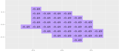

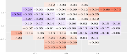
of freedom
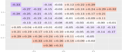
freedom, normal scale
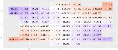
a GARCH(1,1)-model
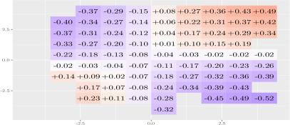
a GARCH(1,1)-model, normal scale
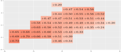
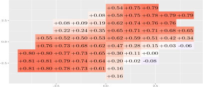
normal scale
For the first example in Figure 3a and 3b, the original scale and the normal scale are almost identical (subject only to the estimation error in the marginal distribution functions), and we see the estimated LGC is close to the true value across all points (in fact the sample Pearson correlation is for these data). Radial and odd reflection symmetry of the LGC, to be discussed in the next subsection, emerge clearly from the estimated values in Figures 3c and 3d. Although and are uncorrelated in the GARCH model, Figures 3e and 3f show strong local dependence, with much the same, although a bit stronger, pattern as for the -distribution, i.e. positive dependence in the first and third quadrant, and negative dependence in the second and fourth quadrant, with increasing dependence away from the center.
For the return data in Figures 3g and 3h we see clearly that the bivariate return distribution is not Gaussian, since in particular there are large local correlations for both large negative and large positive returns. The pattern remains the same on the normal scale. Confidence intervals in such situations can be found in Lacal and Tjøstheim (2017b; 2017a).
We will also illustrate the difference between and by looking at an exchangeable copula with . Several of the standard copulas such as the Clayton, Frank and Gumbel copula are exchangeable. It is shown in Berentsen et al. (2014) that it is possible to compute analytically , and in particular along the curve defined by . If , then the curve reduces to the diagonal . In such a case it is shown in Berentsen et al. (2014) that
| (41) |
where is the standard normal density, where and . Note that and due to exchangeability. It is seen that in addition to the copula , the resulting local Gaussian correlation in (41) also depends on the marginals .
For the -variable version in (40), the cumulative distribution function given by is invariant to transformations of the marginals as detailed above, and in particular by inserting in (41), it follows that along the diagonal
| (42) |
For a parametric copula, the canonical local correlation will depend only on these parameters. In Berentsen et al. (2014) this is used to pinpoint important dependence properties of exchangeable copulas such as the Clayton, Gumbel and Frank copula and copula. Among other things it is shown for the Clayton and Frank copulas that tends to 1 as . Translated to the language of returns of financial variables, this means that if variables are described by the Clayton copula, then for very large negative returns all guarding against risk in a portfolio of and will disappear. Note that for the Gaussian copula, then .
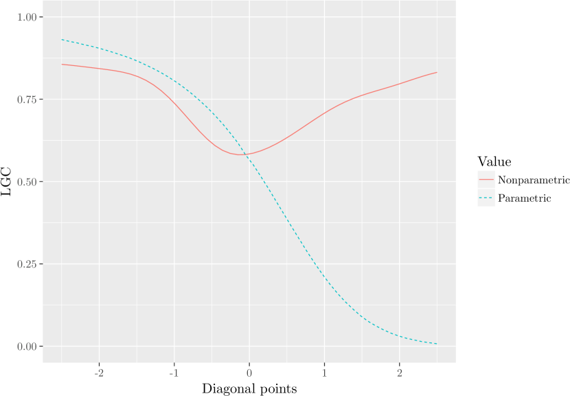
In Figure 4 we have plotted the estimated LGC of the returns (on -scale) on diagonal points, denoted by the label «nonparametric». This curve corresponds to the values along the diagonal through the first and third quadrant in the LGC map given in Figure 3h. We have also estimated the canonical local correlation in (42), by assuming a Clayton copula, estimating the copula parameter. This curve is denoted by the label «parametric» in Figure 4. As we see, this curve is reasonably close to the estimated LGC in the left hand side of the plot (i.e. for negative returns), but as seen, the local Clayton-based correlation goes towards zero on the right hand side of the plot (i.e. for positive returns), whereas the LGC is again increasing. Thus the Clayton copula, which indeed is mostly intended to describe a falling market, does not pick up the dependence patterns for positive returns. The U-shaped LGC of daily returns often occurs. A possible explanation for this, in addition to increasing dependence in a bull market, is that during time periods with a bear market (falling prices), even though the price trend is falling, for some days we actually will see quite large positive daily returns, for example a bear market rally (also known as “sucker’s rally”). These facts may explain why we observe the high local correlation for positive returns too and not just for negative returns. This effect is not typically seen when looking at returns with longer time horizon, e.g. one month. See Støve and Tjøstheim (2014) for further examples.
Another example where an explicit formula for can be obtained is in the parabola model that we have mentioned several times before and where , which gives an intuitive picture of the local dependence properties of this situation where the ordinary Pearson fails so miserably. It is seen that as , if and as and that , which all seem reasonable.
6.2 Some additional properties of the local Gaussian correlation
Before stating particular properties of the LGC, it should be remarked that the family of Gaussian distributions is especially attractive because of its extensive and elegant theory in the multivariate case. Most statisticians will agree that the Gaussian distribution is in a class of itself when it comes to transparency and simplicity of multivariate theory, and this is of course the main reason that it has been so much used in applications, not only in finance but in a host of multivariate problems. But sometimes, and this is certainly the case in econometrics and finance, data do not follow a multivariate Gaussian, and applications based on it can give very misleading results, see Taleb (2007). The point of using the local Gaussian approximation is that one can then move away from Gaussian distributions and describe much more general situations, also multivariate thick tailed distributions like those met in finance. At the same time one can exploit much of the multivariate Gaussian theory locally. We have found this useful in a number of papers extending in various directions: Støve, Tjøstheim, and Hufthammer (2014), Støve and Tjøstheim (2014), Berentsen and Tjøstheim (2014), Berentsen, Kleppe, and Tjøstheim (2014), Berentsen et al. (2014), Berentsen et al. (2017), Lacal and Tjøstheim (2017b), Lacal and Tjøstheim (2017a), Otneim and Tjøstheim (2017), Otneim and Tjøstheim (2018). These results and further extensions will be collected in a forthcoming book, Tjøstheim, Otneim, and Støve (2020).
We will now state some particulars for the local Gaussian correlation as a measure of (local) dependence. We first look at the seven properties (i) - (vii) stated in the beginning of Section 4. These were first stated by Rényi (1959) as desirable properties for a dependence measure to have.
-
(i)
is a local measure, but it is defined for any and under the regularity conditions discussed when defining the population value.
-
(ii)
Because is a local measure we generally have but of course.
-
(iii)
From definitions it follows that and . We believe the possibility to measure negative as well as positive dependence to be one of the main assets of the local Gaussian correlation.
-
(iv)
The condition implies independence of and , but it is not sufficient. Then one must in addition require and for , Tjøstheim and Hufthammer (2013). In the global Gaussian case this is of course trivially fulfilled since all -dependence disappears. Arguably, is a better measure for the dependence between and . (Note that even if we do not necessarily have , and in a bivariate Gaussian approximation. For distributions where this is true, and are independent if and only if ).
-
(v)
If or , then, according to Tjøstheim and Hufthammer (2013), the limiting value as the neighborhood shrinks to the point is equal to 1 or -1, according to or having a positive or negative slope at or . The same is true for a closed curve relationship for a constant , then is equal to 1 or -1 along the curve, depending on whether the tangent at the point has positive or negative slope.
-
(vi)
Like the Pearson the LGC depends on the marginals, but on the -scale, is independent of marginals. Note that in the global case, transformations to standard normals of the margins, the Pearson’s reduces to the van der Waerden rank correlation, Waerden (1952).
-
(vii)
In the Gaussian case we have by construction. Note that this is also true for the Gaussian copula (under monotone transformations of the marginals from normal distributions).
Concerning further properties of the LGC, first note the connection with Lehmann’s quadrant dependence. It is easily shown using the results in that paper that if or for all , then belongs to the class defined in Lehmann’s paper. Moreover, if second moments exist, then for all , implies , and for all implies .
One main asset of Pearson’s is its scale invariance, . There is a corresponding scale invariance for the LGC, but with the proviso that the point is moved to the point . More generally, it is shown by Tjøstheim and Hufthammer (2013) that for a vector and a matrix and for the stochastic variable , then for the local parameter vector at the point , we have and . It follows that we have scale invariance in the following sense .
In Tjøstheim and Hufthammer (2013) the transformation results for have been used to prove a number of symmetry properties. In stating the results we have assumed , because otherwise we may just center the density at , and make statements about symmetry about . These symmetries are illustrated in Figures 3c-3f.
-
(i)
Radial symmetry: If , then , from which , and .
-
(ii)
Reflection symmetry: and/or imply , , , , , .
-
(iii)
Exchange symmetry: If , then and hence .
-
(iv)
Rotation symmetry: Then for a function . If is a spherical density, then satisfies all the symmetry requirements mentioned above. It can be shown that in such a case takes its maximum along the lines and .
In Tjøstheim and Hufthammer (2013) simulations are shown for distributions satisfying these requirements.
6.3 Testing for independence
The LGC can be used for testing independence, and hence as a possible supplement and competitor to the tests in Section 4. A general estimated test functional for testing the independence between two random variables and can be written
| (43) |
where is a measurable function, in general non-negative, and where is the empirical distribution function of . This functional estimates the functionals
and
By choosing the set one can focus the test against special regions, e.g. the tails. One can also pre-test for symmetry properties discussed above and take advantage of those as indicated in Berentsen and Tjøstheim (2014). Such a test can be carried trough in increasing generality as demonstrated in Berentsen and Tjøstheim (2014), and Lacal and Tjøstheim (2017b; 2017a).
Berentsen and Tjøstheim (2014) look at the case of iid pairs and test for independence between and . Lacal and Tjøstheim (2017b; 2017a) consider the time series case where for a time series one can test for independence between and . The corresponding LGC is a function of for a stationary , and it defines a local autocorrelation function. Its estimation theory is covered in Lacal and Tjøstheim (2017b). The theory for the test functional is developed in Lacal and Tjøstheim (2017b; 2017a). From the reasoning in Section 4.5, the asymptotic theory cannot be expected to be very accurate, and they have, as for many (most) of the tests functionals of this type used bootstrapping in tests for serial independence and the block bootstrap for the tests of independence between two time series. In both cases the asymptotic theory for the test functional and the validity of the bootstrap and the block bootstrap have been established. The starting point for the theory is a test functional based on a pairs for the single time series case and pairs for the two time series case. These have been extended in Lacal and Tjøstheim (2017a) to Box-Ljung type of functionals such as
where is of type (43) based on pairs having a lag . Alternatively, they have also used a a test functional
These test functionals have been compared to several other test functionals including Pearson’s and the dcov test. For the simulation experiments tried in Lacal and Tjøstheim (2017b; 2017a) the LGC test functional compares favorably with dcov. As is the case for the dcov it beats the Pearson’s very clearly in non-Gaussian situations, and for the sample sizes used it does not lose much compared to in a Gaussian situation, where is optimal.
References
Aas, Kjersti, Claudia Czado, Arnoldo Frigessi, and Henrik Bakken. 2009. “Pair-Copula Constructions of Multiple Dependence.” Insurance: Mathematics and Economics 44 (2). Elsevier: 182–98.
Abrahams, Julia, and John B. Thomas. 1980. “Properties of the Maximal Correlation Function.” Journal of the Franklin Institute 310 (6): 317–23.
Anderson, Theodore W. 1993. “Goodness of Fit Tests for Spectral Distributions.” The Annals of Statistics 21 (2): 830–47.
Aronszajn, Nachman. 1950. “Theory of Reproducing Kernels.” Transactions of the American Mathematical Society 68 (3): 337–404.
Bartels, Robert. 1982. “The Rank Version of von Neumann’s Ratio Test for Randomness.” Journal of the American Statistical Association 77 (377): 40–46.
Beare, Brendan K. 2010. “Copulas and Temporal Dependence.” Econometrica 78 (1): 395–410.
Beran, Rudolf, Martin Bilodeau, and Pierre Lafaye de Micheaux. 2007. “Nonparametric Tests of Independence Between Random Vectors.” Journal of Multivariate Analysis 98 (9): 1805–24.
Berentsen, Geir Drage, and Dag Tjøstheim. 2014. “Recognizing and Visualizing Departures from Independence in Bivariate Data Using Local Gaussian Correlation.” Statistics and Computing 24 (5): 785–801.
Berentsen, Geir Drage, Ricardo Cao, Mario Francisco-Fernández, and Dag Tjøstheim. 2017. “Some Properties of Local Gaussian Autocorrelation and Other Nonlinear Dependence Measures.” Journal of Time Series Analysis 38 (2): 352–80.
Berentsen, Geir Drage, Tore Kleppe, and Dag Tjøstheim. 2014. “Introducing localgauss, an R-Package for Estimating and Visualizing Local Gaussian Corelation.” Journal of Statistical Software 56 (12): 1–18.
Berentsen, Geir Drage, Bård Støve, Dag Tjøstheim, and Tommy Nordbø. 2014. “Recognizing and Visualizing Copulas: An Approach Using Local Gaussian Approximation.” Insurance: Mathematics and Economics 57: 90–103.
Berlinet, Alain, and Christine Thomas-Agnan. 2004. Reproducing Kernel Hilbert Spaces in Probability and Statistics. Springer.
Berrett, Thomas B, and Richard J Samworth. 2017. “Nonparametric Independence Testing via Mutual Information.” arXiv Preprint arXiv:1711.06642.
Bickel, Peter J., and Murray Rosenblatt. 1973. “On Some Global Measures of the Deviations of Density Function Estimators.” The Annals of Statistics 1: 1071–95.
Billingsley, Patrick. 2008. Probability and Measure. John Wiley & Sons.
Bjerve, Steinar, and Kjell Doksum. 1993. “Correlation Curves: Measures of Association as Function of Covariate Values.” The Annals of Statistics 21 (2): 890–902.
Blomqvist, Nils. 1950. “On a Measure of Dependence Between Two Random Variables.” The Annals of Mathematical Statistics 21 (4): 593–60.
Blum, Julius R., Jack Kiefer, and Murray Rosenblatt. 1961. “Distribution Free Tests of Independence Based on the Sample Distribution Function.” The Annals of Mathematical Statistics 32 (2): 485–98.
Boyer, Brian H., Michael S. Gibson, and Mico Loretan. 1999. “Pitfalls in Tests for Changes in Correlation.” Discussion Paper 597. Federal Reserve Government Papers.
Bradley, Richard C. 1986. “Basic Properties of Strong Mixing Conditions.” Edited by E. Eberlein and M.S. Taqqu. Birkhäuser, Boston, 165–92.
Breiman, Leo, and Jerome H. Friedman. 1985. “Estimating Optimal Transformations for Multiple Regression and Correlation (with Discussion).” Journal of the American Statistical Association 80 (391): 580–619.
Broock, William A., José A. Scheinkman, W. Davis Dechert, and Blake LeBaron. 1996. “A Test for Independence Based on the Correlation Dimension.” Econometric Reviews 15 (3): 197–236.
Carlstein, Edward. 1988. “Degenerate -Statistics Based on Non-Independent Observations.” Calcutta Statistical Association Bulletin 37 (1-2): 55–65.
Chen, Xiaohong, and Yanqin Fan. 2006. “Estimation of Copula Based Semiparametric Time Series Models.” Journal of Econometrics 130 (2): 307–35.
Chen, Yuan, Ying Zeng, Feng Luo, and Yuan Zheming. 2016. “A New Algorithm to Optimize Maximal Information Coefficient.” PLoS ONE 11 (6): e0157567.
Chung, J. K., P. L. Kannapan, C. T. Ng, and P. K. Sahoo. 1989. “Measures of Distance Between Probability Distributions.” Journal of Mathematical Analysis and Applications 138 (1): 280–92.
Chwialkowski, Kacper, and Arthur Gretton. 2014. “A Kernel Independence Test for Random Processes.” In Proceedings of the 31st International Conference on Machine Learning, 32:1422–30.
Csörgö, Sándor. 1985. “Testing for Independence by the Empirical Characteristic Function.” Journal of Multivariate Analysis 16: 290–99.
Czáki, Péter, and János Fischer. 1963. “On the General Notion of Maximal Correlation.” Magyar Tudományos Akad. Mat. Kutató Intézetenk Közlemenényei (Publ. Math. Inst. Hungar: Acad. Sci. 8: 27–51.
Darsow, William F., Bao Nguyen, and Elwood T. Olsen. 1992. “Copulas and Markov Processes.” Illinois Journal of Mathematics 36 (4): 600–642.
Datastream. 2018. Subscription service (Accessed June 2018).
Davis, Richard, Muneya Matsui, Thomas Mikosch, and Phyllis Wan. 2018. “Applications of Distance Correlation to Time Series.” Bernoulli 24 (4A): 3087–3116.
Deheuvels, Paul. 1981a. “A Kolmogorov-Smirnov Type Test for Independence and Multivariate Samples.” Revue Roumaine de Mathemátiques Pures et Appliquées 26 (2): 213–26.
———. 1981b. “An Asymptotic Decomposition for Multivariate Distribution-Free Tests of Independence.” Journal of Multivariate Analysis 11 (1): 102–13.
Delgado, Miguel A. 1996. “Testing Serial Independence Using the Sample Distribution Function.” Journal of Time Series Analysis 17 (3): 271–86.
Denker, Manfred, and Gerhard L. Keller. 1983. “On -Statistics and von Mises’ Statistics for Weakly Dependent Processes.” Zeitschrift Für Wahrscheinlichkeitstheorie Und Verwandte Gebiete 64 (4): 505–22.
Dueck, Johannes, Dominic Edelman, and Donald Richards. 2015. “A Generalization of an Integral Arising in the Theory of Distance Correlation.” Statistics and Probability Letters 97: 116–19.
Dueck, Johannes, Dominic Edelman, Tilmann Gneiting, and Donald Richards. 2014. “The Affinely Invariant Distance Correlation.” Bernoulli 20 (4): 2305–30.
Engle, Robert F. 1982. “Autoregressive Conditional Heteroscedasticity with Estimates of Varaiance of U.K. Inflation.” Econometrica 50 (4): 987–1008.
Escanciano, J. Carlos, and Carlos Velasco. 2006. “Generalized Spectral Tests for the Martingale Difference Hypothesis.” Journal of Econometrics 134 (1): 151–85.
Fan, Yanan, Pierre Lafaye de Micheaux, Spiridon Penev, and Donna Sapolek. 2017. “Multivariate Nonparametric Tests of Independence.” Journal of Multivariate Analysis 153: 189–210.
Ferguson, Thomas S., Christian Genest, and Marc Hallin. 2000. “Kendall’s Tau for Serial Dependence.” Canadian Journal of Statistics 28 (3): 587–604.
Ferraty, Frédéric, and Philippe Vieu. 2006. Nonparametric Functional Data Analysis: Theory and Practice. Springer, New York.
Fisher, Ronald A. 1915. “Frequency Distribution of the Values of the Correlation Coefficient in Samples of an Indefinitely Large Population.” Biometrika 10 (4): 507–21.
———. 1921. “On the Probable Error of a Coefficient of Correlation Deduced from a Small Sample.” Metron 1: 3–32.
Fokianos, Konstantinos, and Maria Pitsillou. 2017. “Consistent Testing for Pairwise Dependence in Time Series.” Technometrics 59 (2): 262–70.
Forbes, Kristin J., and Roberto Rigobon. 2002. “No Contagion, Only Interdependence: Measuring Stock Market Comovements.” The Journal of Finance 57 (5): 2223–61.
Francq, Christian, and Jean-Michel Zakoian. 2011. GARCH Models: Structure, Statistical Inference and Financial Applications. John Wiley & Sons.
Galton, Francis. 1888. “Co-Relations and Their Measurement, Chiefly from Anthropometric Data.” Proceedings Royal Society, London 45 (273–279): 135–45.
———. 1890. “Kinship and Correlation.” North American Review 150 (401): 419–31.
Gebelein, Hans. 1941. “Das Statistische Problem Der Korrelation as Variations - Und Egenwerthproblem Und Sein Zusammengeng Mit Der Ausgleichsrechnung.” ZAMM-Journal of Applied Mathematics and Mechanics/Zeitschrift Für Angewandte Mathematik Und Mechanik 21 (6): 364–79.
Genest, Christian, and Johanna Nešlehová. 2007. “A Primer on Copulas for Count Data.” ASTIN Bulletin 37 (2): 475–515.
Genest, Christian, and Bruno Rémillard. 2004. “Tests of Independence and Randomness Based on the Empirical Copula Process.” TEST 13 (2): 335–69.
Genest, Christian, Kilani Ghoudi, and Bruno Rémillard. 2007. “Rank-Based Extensions of the Brock, Dechert, Scheinkman Test.” Journal of the American Statistical Association 102 (480): 1363–76.
Ghoudi, Kilani, and Bruno Rémillard. 2018. “Serial Independence Tests for Innovations of Conditional Mean and Variance Models.” TEST 27 (1): 3–26.
Ghoudi, Kilani, Reg J. Kulperger, and Briuno Rémillard. 2001. “A Nonparametric Test of Serial Independence for Time Series and Residuals.” Journal of Multivariate Analysis 79 (2): 191–201.
Gorfine, Malka, Ruth Heller, and Yair Heller. 2012. “Comment on “Detecting Novel Associations in Large Data Sets’ by Reshef et al.", Science Dec 16, 2011.”
Gómez, Eusebio, Miguel A. Gómez-Villegas, and J.Miguel Mari’in. 2003. “A Survey on Continuous Elliptical Vector Distributions.” Revista Matemática Computense 16: 345–61.
Granger, Clive, and Jin-Lung Lin. 1994. “Using the Mutual Information Coefficient to Identify Lags in Nonlinear Time Series Models.” Journal of Time Series Analysis 15 (4): 371–84.
Granger, Clive, Esfandiar Maasoumi, and Jeffrey Racine. 2004. “A Dependence Metric for Possible Nonlinear Processes.” Journal of Time Series Analysis 25 (5): 649–70.
Grassberger, Peter, and Itamar Procaccia. 1983. “Measuring the Strangeness of Attractors.” Physica D: Nonlinear Phenomena 9 (1-2): 189–208.
Gretton, Arthur. 2017. “Introduction to RKHS, and Some Simple Kernel Algorithms.” Lecture notes Gatsby Computational Neuroscience Unit.
Gretton, Arthur, and László Györfi. 2010. “Consistent Nonparametric Tests of Independence.” Journal of Machine Learning Research 11 (Apr): 1391–1423.
———. 2012. “Strongly Consistent Nonparametric Test of Conditional Independence.” Journal of Multivariate Analysis 82 (6): 1145–50.
Gretton, Arthur, Olivier Bousquet, Alex Smola, and Bernhard Schölkopf. 2005. “Measuring Statistical Dependence with Hilbert-Schmidt Norms.” In International Conference on Algorithmic Learning Theory, edited by S. Jain, U. Simon, and E. Tomita, 63–77. Springer, Berlin.
Gretton, Arthur, Ralf Herbrich, Alexander Smola, Olivier Bousquet, and Bernhard Schölkopf. 2005. “Kernel Methods for Measuring Independence.” Journal of Machine Learning Research 6 (Dec): 2075–2129.
Hall, Peter. 1992. The Bootstrap and Edgeworth Expansion. Springer, New York.
Hallin, Marc, and Guy Mélard. 1988. “Rank Based Tests for Randomness Against First Order Serial Dependence.” Journal of the American Statistical Association 83 (404): 1117–29.
Hallin, Marc, Jean-François Ingenbleek, and Madan L Puri. 1985. “Linear Serial Rank Tests for Randomness Against ARMA Alternatives.” The Annals of Statistics 13 (3): 1156–81.
Hastie, Trevor, and Rob Tibshirani. 1990. Generalized Additive Models. Chapman; Hall, London.
Heller, Ruth, Yair Heller, and Malka Gorfine. 2013. “A Consistent Multivariate Test of Association Based on Ranks of Distances.” Biometrika 100 (2): 503–10.
Heller, Ruth, Yair Heller, Shachar Kaufman, Barak Brill, and Malka Gorfine. 2016. “Consistent Distribution-Free K-Sample and Independence Tests for Univariate Random Variables.” Journal of Machine Learning Research 17 (1): 978–1031.
Hinich, Melvin J. 1982. “Testing for Gaussianity and Linearity of a Stationary Time Series.” Journal of Time Series Analysis 3 (3): 169–76.
Hjort, Nils Lid, and M. Chris Jones. 1996. “Locally Parametric Nonparametric Density Estimation.” Annals of Statistics 24 (4): 1619–47.
Hoeffding, Wassily. 1940. “Mass-Stabinvariante Korrelationstheorie.” Schriften Des Mathematischen Seminars Und Des Instituts Für Angewandte Mathematik Der Universität Berlin 5 (3): 179–233.
———. 1948. “A Nonparametric Test of Independence.” Annals of Mathematical Statistics 19 (4): 546–57.
———. 1963. “Probability Inequalities for Sums of Bounded Random Variables.” Journal of the American Statistical Association 58 (301): 13–30.
Holland, Paul W, and Yuchung J Wang. 1987. “Dependence Functions for Continuous Bivariate Densities.” Communications in Statistics 16 (3): 863–76.
Hong, Yongmiao. 1998. “Testing for Pairwise Serial Independence via the Empirirical Distribution Function.” Journal of the Royal Statistical Society Series B 60 (2): 429–60.
———. 1999. “Hypothesis Testing in Time Series via the Empirical Characteristic Function: A Generalized Spectral Density Approach.” Journal of the American Statistical Association 94 (448): 1201–20.
———. 2000. “Generalized Spectral Tests for Serial Dependence.” Journal of the Royal Statistical Society Series B 62 (3): 557–74.
Hong, Yongmiao, and Tae-Hwy Lee. 2003. “Inference on Predictability of Foreign Exchange Rates via Generalized Spectrum and Nonlinear Time Series Models.” Review of Economics and Statistics 80 (4): 188–201.
Hong, Yongmiao, and Halbert White. 2005. “Asymptotic Distribution Theory for Nonparametric Entropy Measures of Serial Dependence.” Econometrica 73 (3): 837–901.
Huang, Tzee-Ming. 2010. “Testing Conditional Independence Using Maximal Nonlinear Conditional Correlation.” Annals of Statistics 38 (4): 2047–91.
Ibragimov, Rustam. 2009. “Copula Based Characterizations for Higher-Order Markov Processes.” Econometric Theory 25 (3): 819–46.
Inci, A Can, Hsi-Cheng Li, and Joseph McCarthy. 2011. “Financial Contagion: A Local Correlation Analysis.” Research in International Business and Finance 25 (1): 11–25.
Jentsch, Carsten, Anne Leucht, Marco Meyer, and Carina Beering. 2018. “Empirical Characteristic Functions-Based Estimation and Distance Correlation for Locally Stationary Processes.” Working paper, University of Mannheim.
Joe, Harry. 2014. Dependence Modeling with Copulas. Chapman; Hall, London.
Jones, M. Chris. 1996. “The Local Dependence Function.” Biometrika 83 (4): 899–904.
———. 1998. “Constant Local Dependence.” Journal of Multivariate Analysis 64 (2): 148–55.
Jones, M. Chris, and Inge Koch. 2003. “Dependence Maps: Local Dependence in Practice.” Statistics and Computing 13 (3): 241–55.
Jordanger, Lars Arne, and Dag Tjøstheim. 2017a. “Nonlinear Cross-Spectrum Analysis via the Local Gaussian Correlation.” arXiv Preprint arXiv:1708.02495.
———. 2017b. “Nonlinear Spectral Analysis via the Local Gaussian Correlation.” arXiv Preprint arXiv:1708.02166v2.
Kendall, Maurice G. 1938. “A New Measure of Rank Correlation.” Biometrika 30 (1/2): 81–89.
———. 1970. Rank Correlation Methods. 4th ed. Griffin, London.
King, Maxwell L. 1987. “Testing for Autocorrelation in Linear Regression Models: A Survey.” In Specification Analysis in the Linear Regression Model, edited by M.L. King and D.E.A. Giles, 19–73. Rutledge; Kegan Paul, London.
Kinney, Justin B, and Gurinder S Atwal. 2014. “Equitability, Mutual Information, and the Maximal Information Coefficient.” Proceedings National Academy of Science USA 111: 3354–9.