Comparison of cosmological simulations and deep submillimetre galaxy surveys

Abstract

Recent progress in submillimetre surveys by single-dish telescopes allows us to further challenge the consistency between cosmological simulations and observations. In particular, we compare our simulations that include dust formation and destruction with the recent SCUBA-2 surveys (‘STUDIES’) by putting emphases on basic observational properties of dust emission such as dust temperature, size of infrared (IR)-emitting region, IR luminosity function and IRX–$\beta$ relation. After confirming that our models reproduce the local galaxy properties, we examine the STUDIES sample at $z\approx 1-4$, finding that the simulation reproduces the aforementioned quantities except for the $z\gtrsim 2$ IR luminosity function at the massive end ($\sim 10^{13}$ L_⊙). This means that the current simulation correctly reproduces the overall scaling between the size and luminosity (or star formation rate) of dusty region, but lacks extreme starburst phenomena at $z\gtrsim 2$. We also discuss extinction curves and possible AGN contribution.

1 Introduction

Infrared (IR) observations of galaxies are essential for studying galaxy evolution. Dust grains absorb stellar ultraviolet (UV)-to-optical radiation and reemit it in the IR, thereby strongly modifying the spectral energy distribution (SED) in the UV–IR wavelength range. Therefore the dust emission in galaxies traces the obscured star formation activities, and it accounts for a dominant fraction of star formation activities toward higher redshifts of $z\sim 2$, when the cosmic star formation rate (SFR) peaks in the entire history of the Universe (e.g. Takeuchi et al., 2005; Burgarella et al., 2013, and references therein). Thus, dust extinction and emission are of fundamental importance in deriving the star formation history in the Universe. A large number of IR-detected galaxies are barely visible in the optical and UV (Hwang & Geller, 2013; Calanog et al., 2013).

The luminosity function (LF) is one of the most important properties that represent the statistical nature of galaxies. In particular, the IR LF reflects not only the number density of IR-luminous galaxies, but also the dust abundance in the Universe and the nature of central engines of the luminous sources. Statistical properties of IR-luminous objects have been derived using, for example, the Herschel data. Gruppioni et al. (2013) obtained not only the IR LF at $z=0$ but also its evolution up to $z\sim 4$ (see also Magnelli et al., 2013). The typical detection limit of Herschel survey is $L_{\mathrm{IR}}\sim 10^{11.5}$ L_☉ at $z\sim 1$ and $L_{\mathrm{IR}}\sim 10^{12.5}$ L_☉ at $z\sim 2$.

Clemens et al. (2013) combined Herschel data with Wide-field Infrared Survey Explorer (WISE), Spitzer, and Infrared Astronomical Satellite (IRAS) observations to investigate the properties of a flux-limited sample of local star-forming galaxies. They fit the SEDs with modified blackbody spectra, and showed that they are well-described by dust emission components with emissivity indices $\beta\simeq 2$ and dust temperatures in the range of 10–25 K. They also showed that the dust temperature is strongly influenced by the ratio of SFR to total dust mass of galaxies, indicating that ongoing star formation activities are important for dust heating. Symeonidis et al. (2013) performed a comprehensive study of SEDs and dust temperatures of IR-luminous galaxies at $0.1<z<2$. They used Herschel data from the deepest Spectral and Photometric Imaging Receiver (SPIRE) and Photodetecting Array Camera and Spectrometer (PACS) surveys in the Cosmological Evolution Survey (COSMOS), the Great Observatories Origins Deep Survey (GOODS)-S and GOODS-N fields, and examined the dust properties of IR-luminous ($L_{\rm IR}>10^{10}$ L_⊙) galaxies. They showed that the dust temperatures of galaxies with $L_{\rm IR}\sim 10^{12.5}$ L_⊙ are significantly higher than those with $L_{\rm IR}\sim 10^{10.5}$ L_⊙.

All the above studies have expanded our views on the IR galaxies at high redshift; however, it is important to note that high-$z$ observations by Herschel were strongly affected by the confusion limit (e.g. Koprowski et al., 2017). To obtain a deeper view of dust emission in the Universe, interferometric observations at submillimetre (submm) wavelengths are useful, e.g., by the Atacama Large Millimetre/submillimetre Array (ALMA), which has much higher spatial resolution and sensitivity than Herschel. For example, Fujimoto et al. (2017), using the high-resolution capability of ALMA, indeed constrained the size of dust-emitting region in individual IR-luminous galaxies at $z=0$–6, and found that the IR-emitting region becomes smaller at higher redshift although the dependence is weak. Since the radiation field for a certain luminosity depends on the size of the emitting region, spatially resolving the IR emission is important. Crocker et al. (2018) argued theoretically that the surface brightness of star-forming galaxy cannot exceed $\sim 10^{13}\,\mathrm{L}_{\odot}\,{\rm kpc}^{-2}$, which is determined by the Eddington-limited star formation activity. With the size of dust-emitting region ($\sim 1$ kpc) obtained for IR-luminous objects by Fujimoto et al. (2017), extremely IR-luminous objects ($L_{\rm IR}>10^{13}$ L_⊙) might host a luminosity source other than stars, most probably active galactic nuclei (AGNs).

High spatial resolution is not the only important factor. Because of their narrow field of view, interferometers are generally not suitable for a wide-field survey. Deep surveys with a large ground-based single-dish telescope is a viable way of deriving statistical properties of galaxies up to high redshift. For example, the James Clerk Maxwell Telescope (JCMT) [the Submillimetre Common-User Bolometer Array (SCUBA) on JCMT] was used to investigate the dust properties at various redshifts. Vlahakis et al. (2005) derived the local submm luminosity and dust mass functions by the SCUBA Local Universe Galaxy Survey (SLUGS) and the IRAS Point Source Catalog Redshift Survey (PSCz). The submm observations are suitable for tracing the cold dust component (17–24 K in their sample for $\beta=2$), which usually dominates the total dust mass in galaxies. They showed that, after an appropriate treatment of IR SEDs, the dust mass functions derived from those two surveys agree well.

In general, the IR SED depends not only on the total dust amount but also on the dust temperature. The dust temperature reflects the stellar radiation field incident on the dust; thus, it provides us with important information on the relative spatial distribution of dust to stars. In addition, if we analyze UV attenuation properties, especially based on the UV spectral slope $\beta_{\rm UV}$, we are able to infer how the reddening at UV wavelengths affects the IR luminosity (Meurer et al., 1999). Therefore, a deep survey that satisfies the following conditions is desirable: (i) it covers a large area; (ii) the area is observed at two IR wavelengths (one of the wavelengths should be near the SED peak) so that the derivation of dust temperature is possible; and (iii) the detected galaxies are followed up at rest-frame UV wavelengths. The current deepest survey that satisfies all the above (i)–(iii) is the SCUBA-2 Ultra Deep Imaging EAO Survey (STUDIES) as we introduce below.

The SCUBA-2 camera on JCMT is a powerful instrument for surveying and characterizing the submm emission in the distant Universe with a high simultaneous mapping capability at 450 and 850 $\micron$. STUDIES realized both substantial sensitivity and observing area (Wang et al., 2017). The program has been allocated 650 hours on SCUBA-2 in order to obtain confusion-limited 450 and 850 $\mu$m images in the Cosmic Assembly Near-infrared Deep Extragalactic Legacy Survey (CANDELS) regions in the COSMOS and Subaru/XMM-Newton Deep Survey (SXDS) fields. The program is still ongoing, and it has already produced one of the deepest 450 $\micron$ maps in the COSMOS-CANDELS region. Before STUDIES, the population of known submm galaxies (SMGs) were limited to ultra-luminous ($L_{\rm IR}\gtrsim 10^{12}$ L_⊙) ones for $z>1$ by Herschel (e.g. Gruppioni et al., 2013). By taking advantage of the fast mapping speed of SCUBA-2 and the higher resolution at 450 $\micron$, they claimed that the dust mass function can be derived down to the objects ten times fainter than those detected by Herschel. Wang et al. (2017) showed that the integrated surface brightness from their counts down to 1 mJy is $90\pm 17.2\,{\rm Jy}\,{\rm deg}^{-2}$, which can account for up to $83^{+15}_{-16}$ % of the COBE 450 $\mu$m background. Chang et al. (2018) further showed that the survey can detect $L_{\rm IR}<10^{11}\,{\rm L}_{\odot}$ main-sequence star-forming galaxies up to $z\sim 3$.

Together with the observational advancement, there have also been significant theoretical developments in understanding the dust properties in a cosmological volume. Dayal et al. (2010) implemented models for dust formation by supernovae (SNe) and dust destruction by SN shocks in their cosmological simulation to predict the detectability of dust emission at $z\gtrsim 5$ by ALMA. Popping et al. (2017a) derived the time evolution of the cosmic dust abundance, the dust mass function and the relation between dust-to-gas mass ratio and stellar mass with a semi-analytic model. McKinnon et al. (2017) treated dust as a component associated with gas (treated as a fluid) in their AREPO cosmological hydrodynamical simulations. They broadly reproduced the cosmic dust abundance, the relation between SFR and stellar mass, the relation between dust-to-gas mass ratio and metallicity, and the dust mass function of SMGs. Aoyama et al. (2018, hereafter A18) performed GADGET-3 cosmological hydrodynamic simulations with dust evolution, obtaining cosmic dust abundances at various redshifts consistently with observations. In their simulation, the chemical evolution code CELib (Saitoh, 2017) was coupled with the models of star formation, SN feedback, metal enrichment, dust formation and its destruction. The dust grain size distribution was treated by the ‘two-size approximation’, in which large and small grains are separated at $\sim 0.03\,\mu$m (Hirashita, 2015). This two-size approximation has also been applied to a simulation of galaxy clusters by Gjergo et al. (2018), who confirmed the importance of dust processing in the gas. McKinnon et al. (2018) followed up their earlier work with an implementation of the evolution of grain size distribution in isolated galaxy simulations, providing some test calculations. Thus, for cosmological simulations, the two-size approximation has been the most advanced way of implementing the grain size information so far.

Since the extinction properties of UV stellar light strongly depend on the grain size distribution (Asano et al., 2014), A18’s simulation based on the two-size approximation provides a unique tool that predicts the extinction curves in individual galaxies in a cosmological volume. Therefore, among the simulations that explicitly include dust evolution, A18’s work is the most suitable for the comparison with recent deep submm surveys. The only caveat is the poor spatial resolution, which is unavoidable for a cosmological simulation that attempts to simulate a large sample of galaxies simultaneously. However, as shown later, we resolve the observationally suggested size of IR-emitting region $\sim 1$ kpc (Fujimoto et al., 2017) at high redshift. We also test our models against the observational data at $z=0$, and confirm that our simulation reproduces the observed properties of dust in the local Universe. Thus, the aim of this paper is to examine the consistency between the state-of-the-art large-volume simulation of dust enrichment and the deepest observation of statistical dusty-galaxy properties.

In addition, taking advantage of the implementation of grain size distribution in our simulations and the existence of rest-UV follow-ups for the observational data, we consider the so-called IRX–$\beta_{\mathrm{UV}}$ relation. The relation between IR excess (IRX: UV-to-IR luminosity ratio) and $\beta_{\rm UV}$ was originally obtained by Meurer et al. (1999) for nearby starburst galaxies. Theoretically, $\beta_{\rm UV}$ can be predicted by a stellar population synthesis model with dust extinction included. The IRX–$\beta_{\mathrm{UV}}$ relation is observationally useful because it enables us to infer what fraction of star formation activity is attenuated by dust (e.g. Hao et al., 2011; Reddy et al., 2012; Smit et al., 2012; Finkelstein et al., 2012; Bouwens et al., 2014). The IRX–$\beta_{\mathrm{UV}}$ relation is still being debated. Takeuchi et al. (2012) reconsidered the IRX–$\beta_{\rm UV}$ relation by correcting it for the photometric aperture effect, and obtained a ‘shifted’ IRX–$\beta_{\mathrm{UV}}$ relation relative to that derived by Meurer et al. (1999). There is also an indication that the IRX–$\beta_{\mathrm{UV}}$ relation is different at $z\gtrsim 5$ (Capak et al., 2015; Bouwens et al., 2016). Some theoretical models of IRX–$\beta_{\mathrm{UV}}$ relation show that the relation is affected by the contamination of old stars and the relative distribution of dust and stars (or radiation transfer effects) (Mancini et al., 2016; Ferrara et al., 2017; Narayanan et al., 2018; Popping et al., 2017b).

This paper is organized as follows. We introduce the simulation and the analysis method in Section 2. We test our results against observational data at $z=0$ in Section 3. In Section 4, we compare the simulation results at $z=1$–4 with the STUDIES galaxy survey data. In Section 5, we further discuss this comparison, including the uncertainties and limitations. Section 6 concludes this paper. We adopt the following cosmological parameters (Planck Collaboration et al., 2016): baryon density parameter $\Omega_{\rm b}=0.049$, total matter density parameter $\Omega_{\rm m}=0.32$, cosmological constant parameter $\Omega_{\Lambda}=0.68$, Hubble constant $H_{0}=67$ km s^-1 Mpc^-1, power spectrum index $n_{\rm s}=0.9645$, and density fluctuation normalisation $\sigma_{8}=0.831$. In this paper, we also use $h\equiv H_{0}/(100$ km s^-1 Mpc${}^{-1})=0.67$ for the non-dimensional Hubble constant.

2 MODEL

2.1 Cosmological simulation with dust evolution

Table 1: Simulation Parameters

Name	Boxsize	$N$	$\varepsilon_{\rm grav}$	$m_{\rm dm}$	$m_{\rm gas}^{\rm init}$
	[$h^{-1}$Mpc]		[$h^{-1}$kpc]	[$h^{-1}{\rm M}_{\odot}$]	[$h^{-1}{\rm M}_{\odot}$]
L50N512	50	$2\times 512^{3}$	3	$6.89\times 10^{7}$	$1.28\times 10^{7}$
L25N512	25	$2\times 512^{3}$	1.6	$8.61\times 10^{6}$	$1.60\times 10^{6}$

Note: $N$, $\varepsilon_{\rm grav}$, $m_{\rm dm}$ and $m_{\rm gas}^{\rm init}$ are the total number of particles, the gravitational softening length, the mass of dark matter particle and the initial mass of gas particle, respectively.

We use and post-process the simulation of A18 to derive the statistical dust emission properties in a cosmological volume. We briefly review the simulation here. We performed cosmological $N$-body/smoothed particle hydrodynamic (SPH) simulations with gadget3-osaka developed by Aoyama et al. (2017) and Shimizu et al. (2019, in preparation) based on the gadget-3 code (originally described in Springel, 2005). Important parameters for the simulation setup are summarized in Table 1, and L50N512 is our default simulation.

In addition to the L50N512 run in A18, we also performed another simulation, referred to as L25N512, with a smaller box size in order to test the effect of spatial resolution (Table 1). However, the number of galaxies whose luminosities are in the range of the adopted observational sample decreases because of the 8 times smaller volume. Therefore, L25N512 is not very suitable for our main comparison with the observations, and is only used to examine the effect of spatial resolution. We also find that the effective resolution of L50N512 (sub-kpc) is sufficient for resolving the IR-luminous regions (Section 3.1), but twice worse spatial resolution would fail to resolve them. Note that we allow the SPH smoothing length to become as small as one-tenth of the gravitational softening length. For example, the minimum SPH smoothing in the L50N512 run has decreased to 0.84 kpc and 0.3 kpc (both physical) for $z=0$ and $z=3$, respectively. Therefore, considering the currently available computational resource, L50N512 is the optimum setup in terms of box size and resolution. In other words, we are able to clarify how much such an ‘optimum’ simulation could reproduce the observational properties of IR-selected galaxies, and extract physical information through the comparison with observations.

In order to clarify the resolution effects of simulations, A18 also compared dust mass functions between L50N512 and a lower resolution simulation with $2\times 256^{3}$ particles. There were no significant differences between the two results. We also confirmed that the basic relations between the dust abundance and other physical quantities do not significantly change between the low- and high-resolution runs. Thus, the convergence of dust properties has already been confirmed. In the following, we display the results from L50N512 run unless otherwise stated.

We treat star formation, SN explosion, stellar feedback, and metal enrichment by SNe and asymptotic giant branch stars consistently using CELib (Saitoh, 2017). We solve the dust evolution on each gas particle. In order to calculate the grain size distribution within a reasonable computational cost, we adopt the two-size approximation, in which the entire grain size range is represented by two sizes divided at grain radius $a\sim 0.03\,\mu$m (Hirashita, 2015). The following processes are included for dust evolution: dust condensation in stellar ejecta, dust growth in the dense and cold gas via accretion and coagulation, dust disruption (or fragmentation) by shattering in the diffuse medium, dust destruction by sputtering in SN shocks and hot inter-galactic medium (IGM). The simulation is not capable of resolving dense clouds in which dust grains grow via accretion and coagulation. Thus, A18 adopted a subgrid model where each gas particle satisfying the ‘dense-gas condition’ (number density $n_{\mathrm{gas}}>0.1$ cm^-3 and temperature $T_{\mathrm{gas}}<10^{4}$ K) hosts dense clouds with $n_{\mathrm{gas}}=10^{3}$ cm^-3 and $T_{\mathrm{gas}}=50$ K (the mass fraction of the dense clouds in the gas particle is assumed to be 10 per cent). For stellar dust enrichment, we assume that 10 per cent of the metals condense into dust. For the other processes, we adopt proper time-scales for large and small grains basically estimated from the collision time-scales between dust grains or between dust and gas, depending on the process. These time-scales generally depend on gas density, temperature, and metallicity (see Sections 2.2–2.4 of A18 for detailed descriptions of each process).

Galaxies are identified using P-Star groupfinder (Springel et al., 2001). In short, we find the baryonic (gas + stars) density peaks in the smoothed density field and measure the densities of $N_{\rm ngb}$ nearest neighbour particles around the density peak. We adopt $N_{\rm ngb}=512$ and $N_{\rm ngb}=128$ for L50N256 and L25N512, respectively. The particle at the density peak is considered as a ‘head particle’ around which a galaxy is identified if all the neighbor particles have lower densities.

The most basic quantities in individual galaxies are the masses of dust and stars, which are needed to treat the absorption and reprocessed of stellar light by dust. The spatial extent of dust and stars is also important since the heating of dust by the radiation field depends on how compactly dust and stars are distributed. We find that the radial profile of dust mass density in a galaxy is approximately described by an exponential function in our simulation, which provides the scale length $R_{\rm dust}$. In order to estimate $R_{\mathrm{dust}}$, we extract the (20 comoving kpc)³ cubic region around each galaxy centre. We cut each region into $20^{3}$ cubic grid. Thus the effective resolution of the radial profile estimate is 1 kpc, which is comparable to the spatial resolution of our simulation. By fitting the profile to an exponential function with the least-square method, we obtain the scale length $R_{\mathrm{dust}}$, and adopt it as the radius of dusty region.

To estimate the optical depth of dust, we first estimate the surface densities of large and small grains, denoted as $\Sigma_{\rm L}$ and $\Sigma_{\rm S}$, respectively, in the following manner:

$$M_{\mathrm{L/S}} = \int_{0}^{\alpha R_{\mathrm{dust}}}4\pi R^{2}\rho_{\mathrm{L/S}}\,\mathrm{d}R,$$ (1)

$$\Sigma_{\rm L/S} = \dfrac{M_{\rm L/S}}{\pi(\alpha R_{\rm dust})^{2}}~{},$$ (2)

where $M_{\mathrm{L}}$, $M_{\mathrm{S}}$, $\rho_{\mathrm{L}}$, and $\rho_{\mathrm{S}}$ are the total mass of large grains, the total mass of small grains, the mass density of large grains, and the mass density of small grains, respectively. The parameter $\alpha$ determines the radial range where the total dust mass is derived. We later fix the value of $\alpha$ in Section 3.1. The total dust mass, $M_{\mathrm{dust}}$, is defined as

$$M_{\mathrm{dust}}=M_{\mathrm{L}}+M_{\mathrm{S}}.$$ (3)

2.2 Estimation of dust extinction optical depth

Dust extinction including its wavelength dependence (extinction curve) is estimated based on the surface densities of large and small grains in equation (2). For the calculation of extinction curve, we need a continuous functional form of grain size distribution while we represent the entire grain size range by two sizes. Following Hirashita (2015) and Hou et al. (2017), we adopt the ‘modified-lognormal function’ of grain size distribution for large and small grains:

$$N_{i}(a) = \dfrac{C_{i}}{a^{4}}\exp\left(-\dfrac{\left(\ln(a/a_{0,i})\right)^{2}}{2\sigma^{2}}\right)~{},$$ (4)

where $a$ is the grain radius (we assume grains to be spherical), $i=\mathrm{L}$ or S is the label for large or small grains, $C_{i}$ is the normalization constant, $a_{0,i}$ is the typical grain radius of each size domain (we adopt $a_{0,{\rm L}}=0.1\,\mu{\rm m}$ and $a_{0,{\rm S}}=0.005\,\mu{\rm m}$), and $\sigma$ is the standard deviation of the lognormal distribution. The normalization $C_{i}$ is determined in a consistent manner with the total surface densities estimated in Eq. (2) as

$$\Sigma_{i} = \displaystyle\int_{0}^{\infty}\dfrac{4}{3}\pi a^{3}sN_{i}(a)\,\mathrm{d}a,$$ (5)

where $s$ is the material density of dust grains. We adopt $s=3$ g cm^-3.

We calculate the optical depth $\tau_{\lambda}$ and the extinction curve $A_{\lambda}$ (magnitude of extinction as a function of wavelength) as follows:

$$\tau_{\lambda} = \displaystyle\sum_{i={\rm L,S}}\displaystyle\int_{0}^{\infty}N_{i}(a)\pi a^{2}Q_{\rm ext}(a,\lambda)\,\mathrm{d}a~{},$$ (6)

$$A_{\lambda} = (2.5\log_{10}\mathrm{e})\tau_{\lambda}~{},$$ (7)

where $Q_{\rm ext}(a,\lambda)$ is the extinction cross-section relative to the geometric cross-section, which is evaluated by using the Mie theory (Bohren & Huffman, 1983). For the optical constants necessary for the Mie theory calculation, we need to specify the grain materials. However, in our simulation, we do not separate grain species. Thus, we simply assume that all grains are composed of silicate, for which we adopt the same optical constants as in Weingartner & Draine (2001). To avoid the complexity in the prediction arising from the 2175 Å bump, we neglect graphite. Neglecting graphite empirically gives a good fit to the Small Magellanic Cloud (SMC) extinction curve (Pei, 1992; Weingartner & Draine, 2001; Hou et al., 2016). In other words, our model assumes a bumpless extinction curve, which will explain the observational data well, as we show later. We emphasize that the steepness of extinction curve can still be estimated in a manner consistent with the calculated grain size distribution. We discuss the resulting extinction curves in Section 5.3.

2.3 Stellar SED and dust emission

We now calculate the stellar SED for each galaxy taking into account the extinction optical depth estimated in equation (6). We adopt a spectral synthesis model by Bruzual & Charlot (2003) to obtain the intrinsic SED of single stellar population at various ages. The SED per stellar mass of single stellar population is denoted as $\tilde{L}_{\lambda}$, which depends on the stellar age ($t_{*}$) and metallicity ($Z_{*}$). We adopt the Chabrier initial mass function (IMF) (Chabrier, 2003). The intrinsic stellar SED, $L_{\lambda}^{0}$, is calculated by summing up all the contribution from the stellar particles within the radius $R_{\mathrm{dust}}$ as ($k$ is the index of stellar particle)

$$L_{\lambda}^{0} = \displaystyle\sum_{\begin{subarray}{c}k\\ 0\leq R_{k}\leq\alpha R_{\rm dust}\end{subarray}}\!\!\!\!\!\tilde{L}_{\lambda}(t_{*(k)},\,Z_{*(k)})m_{{\rm star}(k)},$$ (8)

where $m_{{\rm star}(k)}$ and $R_{k}$ are the mass and the distance from the galaxy centre for the $k$-th stellar particle. The observed SED after dust extinction is calculated by

$$L_{\lambda}=\left\{\begin{array}[]{ll}L_{\lambda}^{0}{\displaystyle\frac{1-\exp(-\tau_{\lambda})}{\tau_{\lambda}}}&\mbox{(for $\lambda>912$\,\AA)},\\ 0&\mbox{(for $\lambda\leq 912$\,\AA)},\\ \end{array}\right.$$ (11)

where we assume a mixed geometry between dust and stars (which gives a better approximation for the dust–star geometry within $\alpha R_{\mathrm{dust}}$ than a screen geometry) and complete absorption of ionizing photons ($\lambda\leq 912$ Å) by hydrogen. We use $\tau_{\lambda}$ calculated in equation (6). We assume that the extinguished light is reprocessed into the IR regime:

$$L_{{\rm IR}} = \displaystyle\int_{912\,\text{\AA}}^{\infty}(L_{\lambda}^{0}-L_{\lambda})\,\mathrm{d}\lambda~{},$$ (12)

where $L_{\mathrm{IR}}$ is the total IR luminosity, which is directly compared with the observationally derived IR luminosity at rest-frame $\lambda=8$–1000 $\micron$ by assuming that the dust luminosity emitted at wavelengths shorter than 8 $\micron$ or longer than 1000 $\micron$ is negligible.

2.4 Derivation of dust temperature

For simplicity, we assume that the dust emission follows the so-called modified blackbody spectrum with a single dust temperature $T_{\mathrm{dust}}$ (i.e. we neglect the variation of dust temperature within a galaxy). With this simplification, the IR SED $L_{\nu}^{\rm IR}$ is described by the following equations:

$$L_{\nu}^{\rm IR} = 4\pi M_{\rm dust}\kappa_{\nu}B_{\nu}(T_{\rm dust})~{},$$ (13)

$$\kappa_{\nu} = \kappa_{0}\left(\frac{\nu}{\nu_{0}}\right)^{\beta},$$ (14)

where $B_{\nu}(T)$ is the Planck function, $\kappa_{\nu}$ is the mass absorption coefficient at frequency $\nu$, $T_{\mathrm{dust}}$ is the dust temperature, and $\kappa_{0}$ is the value of $\kappa_{\nu}$ at frequency $\nu_{0}$. We adopt $\nu_{0}=3.00\times 10^{12}$ Hz and $\kappa_{0}=52.2$ cm² g^-1 (Dayal et al., 2010). Since $T_{\mathrm{dust}}\propto\kappa_{0}^{-1/(4+\beta)}$ under a fixed $L_{\mathrm{IR}}$, the resulting dust temperature is not sensitive to the adopted value of $\kappa_{0}$. With the above SED shape, the total IR luminosity $L_{\rm IR}$ is evaluated as (e.g. Dayal et al., 2010)

$$L_{\rm IR} = \displaystyle\int_{0}^{\infty}L_{\nu}^{\rm IR}\mathrm{d}\nu$$

$$= 4\pi M_{\rm dust}\kappa_{\nu_{0}}\nu_{0}^{-\beta}\left(\dfrac{k_{\rm B}T_{\rm dust}}{h}\right)^{4+\beta}\left(\dfrac{2h}{c^{2}}\right)\Gamma(4+\beta)\zeta(\beta+4)~{},$$

where $\Gamma(x)$ and $\zeta(x)$ are the Gamma function and the Riemann zeta function, respectively, and $k_{\rm B}$, $h$ and $c$ are the Boltzmann constant, the Planck constant and the speed of light, respectively. We assume radiative equilibrium for dust grains in order to derive the dust temperature, so that we substitute equation (12) for $L_{\mathrm{IR}}$ in equation (LABEL:eq:integ_LIR). By solving equation (2.4) for $T_{\rm dust}$, we obtain (Shimizu et al., 2012)

$$T_{\rm dust} = \dfrac{h}{k_{\rm B}}\left(\dfrac{c^{2}\nu_{0}^{\beta}}{8\pi h\kappa_{0}\Gamma(4+\beta)\zeta(4+\beta)}\dfrac{L_{\rm IR}}{M_{\rm dust}}\right)^{\dfrac{1}{4+\beta}}.~{}$$ (16)

We adopt $\beta=2$ unless otherwise noted (Clemens et al., 2013). In this case, equation (16) is reduced to

$$T_{\rm dust} = 7.5\left(\dfrac{L_{\rm IR}/L_{\odot}}{M_{\rm dust}/M_{\odot}}\right)^{\dfrac{1}{6}}~{}{\rm K}~{}.$$ (17)

2.5 IRX-$\beta_{\rm UV}$ relation

The IRX is defined as

$${\rm IRX} \equiv \dfrac{L_{\rm IR}}{L_{\mathrm{UV}}(1650\AA)},$$ (18)

where $L_{\mathrm{UV}}(\lambda)\equiv\lambda L_{\lambda}$ and we adopt $\lambda=1650$ Å following the UV wavelength of the STUDIES sample (see Section 4.1). The UV SED slope, $\beta_{\rm UV}$, which is defined by the relation $L_{\lambda}\propto\lambda^{\beta_{\rm UV}}$ at rest-UV wavelengths, is estimated as

$$\beta_{{\rm UV}} = \dfrac{\log_{10}(L_{\lambda_{2}})-\log_{10}(L_{\lambda_{1}})}{\log_{10}(\lambda_{2})-\log_{10}(\lambda_{1})}~{},$$ (19)

where $\lambda_{1}$ and $\lambda_{2}$ are fixed to 1650 Å and 2300 Å, respectively, for the comparison with the STUDIES sample.

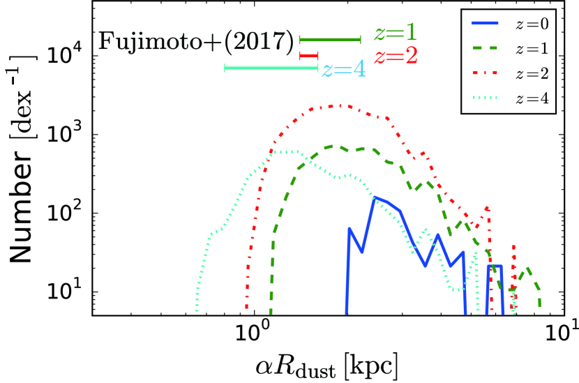
Figure 1: Histogram of the radius ($\alpha R_{\mathrm{dust}}$) of IR-emitting region at $z=0$, 1, 2, and 4 (solid, dashed, dot-dashed, and dotted lines, respectively) for the galaxies in the simulation box. We adopt $\alpha=2$ in this paper; that is, the IR-emitting region is twice the scale length of the dust distribution. We selected galaxies whose IR luminosity is greater than $10^{11}{\rm L}_{\odot}$. The horizontal bars show the corresponding observed ranges at $z=1$, 2, and 4 taken from Fujimoto et al. (2017). We find that $\alpha=2$ produces the radii consistent with the observed results including the evolution along the redshift.

3 Calibration and Tests

Before comparison with the STUDIES sample, we check if our models reproduce the principal properties of dust emission at $z=0$. In the above, the radius of the IR-emitting regions relative to the scale length of dust distribution ($\alpha$ in equation 2) was left undetermined. We first determine it in Section 3.1. For the statistical properties of dust emission, we focus on the IR LF. We also examine the $T_{\rm dust}$–$L_{\rm IR}$, $R_{\rm dust}$–$L_{\rm IR}$ and IRX–$\beta_{\rm UV}$ relations. The dust mass and its relation to the metallicity have already been tested by A18; thus, we concentrate on the IR emission properties in this paper.

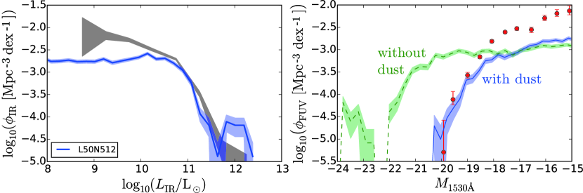
Figure 2: Left panel: IR LF in the simulation at $z=0$ with the shaded region showing the Poisson error. The grey shaded region indicates the IR LF obtained by Herschel with 1 $\sigma$ uncertainty (Gruppioni et al., 2013). Right panel: Rest-frame UV LF in the simulation at $z=0$. The solid and dashed lines show the results with and without dust extinction. The blue and green shaded regions show the Poisson error. Observational result from GALEX is shown as red points with error bars (Treyer et al., 2005).

3.1 Radius of IR-emitting region

In our simulation, the radius of IR-emitting region is assumed to be $\alpha$ times the scale length of dust distribution ($R_{\mathrm{dust}}$). We determine $\alpha$ to reproduce the observed IR-emitting region sizes of IR-luminous galaxies with $L_{\mathrm{IR}}\gtrsim 10^{12}$ L_☉. We find that $\alpha=2$ can reproduce the ALMA measurement of IR-emitting region sizes in Fujimoto et al. (2017) as shown in Fig. 1; we compare the distribution of $\alpha R_{\mathrm{dust}}$ with $\alpha=2$ for the simulated galaxies whose IR luminosity is greater than $10^{11}\,{\rm L}_{\odot}$ with the observational data at $z=1$–4. We find that our dust-emitting region radii agree not only with the observations at a particular redshift, but also with the observed decreasing trend towards higher redshifts. This comparison shows that our simulation captures the redshift evolution of dust-emitting region consistently with the current observation. Because $\alpha R_{\mathrm{dust}}$ is important in determining the dust optical depth (or the dust surface density; equations 2 and 6), the consistency in $R_{\mathrm{dust}}$ confirms that our simulation can give a reasonable estimate for the dust optical depth under a given dust mass.

3.2 IR LF

The IR LF is significantly affected by the dust abundance and the stellar populations of galaxies. Thus, comparison of the IR LF in the simulation with the observed one is useful to test our treatment of dust evolution and star formation as shown in Fig. 2, where we compare our simulation results with the observational data obtained by Herschel at $z=0$ (Gruppioni et al., 2013). The IR LF is also derived from other IR observations (e.g. Kilerci Eser & Goto 2018 for a recent ‘accurate’ IR LF). Since recently obtained IR LFs at $z\sim 0$ are consistent with the previous results within the uncertainty of our theoretical estimates of $L_{\mathrm{IR}}$, we only focus on the Herschel data in this paper.

We also compared the UV LF at $z\simeq 0$ with a corresponding observational result (GALEX; Treyer et al., 2005) in Fig. 2. We observe a good agreement at the bright-end of $M_{1530}<-19$, where $M_{1530}$ is the rest-frame UV magnitude at 1530 Å. However we underestimate the number of UV faint objects at $M_{1530}>-19$ by 0.5 dex at most. This is because the low-mass galaxies in our simulation is not so active in star formation. We also show the intrinsic UV LF (before applying dust extinction) in Fig. 2 in order to show the impact of dust. If dust extinction effect is not considered, then the bright end of UV LF is overestimated and the observed data points cannot be explained. We emphasize that the dust extinction correctly suppresses the UV luminosity at the bright end, which is important in our studies of IR-luminous galaxies.

There is a bump in the IR LF at $L_{\rm IR}\simeq 10^{12}\,L_{\odot}$, which corresponds to the bump at $M_{1530}\simeq-23.5$ in the intrinsic UV LF. This bump is created by just a few objects in the simulation box. In this simulation, the star formation in some massive galaxies is not quenched even in the low-$z$ Universe. However, this bump does not affect the conclusion of this paper because the number of such massive galaxies is very small.

Our simulation reproduces the observed IR LF within a factor of 3 at $z=0$, although the simulated LF is lower than the observed data at the faint end. The overall match of LF indicates that our model is ‘calibrated’ roughly by the local observation in a statistical sense. In other words, the total IR emissivity in a cosmological volume is correctly modeled in our simulation; i.e., the total fraction of stellar light absorbed by dust is appropriately modeled. This success at $z=0$ gives a basis on which we discuss the LFs at other redshifts.

We also investigated the relation between $L_{\rm IR}$ and $\mathcal{D}_{\rm tot}$. $\mathcal{D}_{\rm tot}$ and $L_{\rm IR}(z)$ are correlated at all redshifts ($z<5$). $L_{\rm IR}(z)=10^{12}\,L_{\odot}$ corresponds to $\mathcal{D}_{\rm tot}=0.01$. When one fixes $\mathcal{D}_{\rm tot}$, $L_{\rm IR}(z)$ decreases as the redshift increases. The reason is that the stellar population becomes older as the redshift becomes smaller.

However, the LF only provides a statistical aspect of the dust emission properties. In the following subsections, we examine the relations among quantities characteristic of dust emission in individual galaxies at $z=0$.

3.3 $T_{\rm dust}-L_{\rm IR}$ relation

Dust temperature depends on the total radiative energy incident on the dust. Therefore, the $T_{\rm dust}-L_{\rm IR}$ relation gives us a useful clue as to how the increase of dust emission is associated with the increase of dust heating. In Fig. 3, we compare the $T_{\rm dust}-L_{\rm IR}$ relation in the simulation with the observational data for local galaxies (Clemens et al., 2013; Zavala et al., 2018). We successfully and quantitatively reproduce the observed trend of rising $T_{\mathrm{dust}}$ with increasing $L_{\mathrm{IR}}$ seen for most of the sample. This means that the stellar radiation field incident on the dust (or the spatial distribution of stars and dust) is appropriately modeled in the simulation.

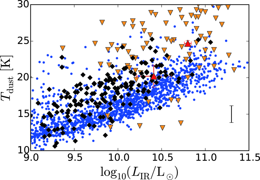
Figure 3: Relation between dust temperature and IR luminosity at $z=0$. The simulated galaxies are represented by the blue points. The black diamonds, orange inverted triangles and red triangles are taken from Clemens et al. (2013), Amblard et al. (2010) and Zavala et al. (2018), respectively. The typical observational uncertainty of the dust temperature is shown in the bottom right corner (Clemens et al., 2013).

3.4 IRX–$\beta_{\rm UV}$ relation

Finally, we examine the IRX–$\beta_{\mathrm{UV}}$ relation, which connects the dust extinction and emission properties. As shown in Fig. 4, our simulation shows a rising trend of IRX and $\beta_{\mathrm{UV}}$, which roughly agrees with the observed trends represented by Meurer et al. (1999), Takeuchi et al. (2012) and Casey et al. (2014) (see also references therein). A significant fraction of galaxies are distributed around the curves which are obtained for a nearby galaxy sample. A large part of objects with low stellar mass ($10^{8}\lesssim M_{\ast}/{\rm M}_{\odot}\lesssim 10^{9}$; dark blue points in Fig. 4) have low IRX and relatively red SEDs because the dust-to-gas mass ratio of these galaxies is small ($\mathcal{D}_{\rm tot}\lesssim 10^{-3}$) (i.e. the dust extinction is small) and the current star formation activity is low (i.e. the stellar colour is red) in our simulation.

There are several very actively star-forming galaxies seen in their extremely blue colours around $\beta_{\rm UV}\simeq-3$. They are dust-poor low-mass systems whose stellar light is dominated by a very young ($\sim 10^{6}$ yr) stellar population and is little extinguished by dust. Massive starburst galaxies show high IRX ($\gtrsim 10$) and $\beta_{\mathrm{UV}}$ between $\sim-2$ and $-1$. The narrow range of $\beta_{\mathrm{UV}}$ is due to the limit of $\beta_{\rm UV}$ in the mixed dust geometry as we discuss in Section 5.2 (and Appendix A). Thus, the range of $\beta_{\mathrm{UV}}$ for those massive starbursts may be underestimated. If we assume a screen geometry, the data points are distributed over a wider range of $\beta_{\mathrm{UV}}$, but the IRX of some galaxies also becomes extremely high (up to $10^{6}$; such a high number is not observed). Probably, the real geometry of dust distribution is in the middle of these two extremes (mixed and screen). Since we do not resolve the detailed dust distribution, we do not tune the dust geometry. We only emphasize that we obtain the IRX–$\beta_{\mathrm{UV}}$ relation broadly consistent with the observed one.

4 Comparison with the STUDIES Sample

4.1 Observational data

We compare our simulation results with the high-redshift observational sample obtained by the STUDIES project. We adopt deep submm imaging surveys that have been carried out in the COSMOS field with SCUBA-2 by various teams (Casey et al., 2013; Geach et al., 2013, 2017; Wang et al., 2017) at 450 and 850 $\micron$. Casey et al. (2013) performed a large and uniform blank-field survey over a large scan area of $\sim 15^{\prime}\times 15^{\prime}$ with a noise level of $\sim 3.6$ mJy at 450 $\micron$. The SCUBA-2 Cosmology Legacy Survey (S2CLS; Geach et al., 2013, 2017) and the SCUBA-2 Survey of SMGs in the COSMOS field (S2COSMOS; Simpson et al. in preparation) covered several well studied extragalactic legacy fields. We adopt the deep blank-field survey in the COSMOS field. The noise level at the deepest regions of this survey is $\sim 0.9$ mJy at 450 $\micron$. Finally, STUDIES (Wang et al., 2017) is an ongoing JCMT Large Program that aims at reaching the confusion limit in the COSMOS-CANDELS field. The current r.m.s noise at the deepest regions of this image is $\sim 0.75$ mJy. After combining all these data, the extremely deep image leads to a sample of 269 galaxies selected at 450 $\micron$ (see, e.g., Chang et al., 2018), with a redshift range of $0.21<z<4.37$ (median $z=1.64$). In addition to the dataset of STUDIES, we also use the observational data obtained by another SCUBA-2 project with a comparable capability (Zavala et al., 2018) and a representative Herschel program (Casey et al., 2014) for reference. Note that these two samples give consistent conclusions to those derived from the STUDIES sample as we see below.

Since the COSMOS field has been surveyed at other wavelengths, Lim et al. (in preparation; see also Chang et al. 2018) used those data to derive physical properties of the sources with SED fitting in the optical and IR. As a consequence, they succeeded in deriving the relations between the quantities that we considered in the previous section such as IRX, $\beta_{\rm UV}$, dust temperature, and IR luminosity. The sample provides us with an opportunity of comparing our theoretical results with a uniform sample (sample collected by a uniform method), so that we do not have to worry about systematic difference between different samples. We should keep in mind that the sample we adopt is IR-selected: Those submm sources are usually optically faint mainly because they are heavily obscured by dust.

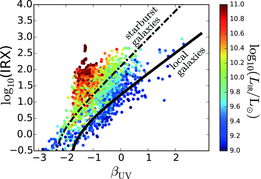
Figure 4: IRX–$\beta_{\rm UV}$ relation at $z=0$. The colour of each point shows the logarithmic IR luminosity in units of ${\rm L}_{\odot}$ as shown by the colour bar. We show the fitting formulae of IRX–$\beta_{\rm UV}$ for starburst galaxies (dot–dashed line; Kong et al., 2004) and galaxies in the local Universe (solid line; Takeuchi et al., 2012).

Below we compare the IR-emitting properties of the simulated galaxies at various redshifts to the above observational sample. We consider the redshift ranges $0.5<z<1.5$, $1.5<z<2.5$, $2.5<z<3.5$, and $3.5<z<4.5$, where the observed LFs are derived with sufficient statistical significance. We adopt the simulation snapshots at $z=1$, 2, 3, and 4 for comparison.

4.2 $M_{*}$–$L_{\mathrm{IR}}$ relation

Before examining the dust emission properties, it is useful to clarify the stellar mass ($M_{*}$) in the IR luminosity range covered by the STUDIES sample. In Fig. 5, we show the relation between IR luminosity and stellar mass of each galaxy in the simulation. Although the scatters are large, there is a clear correlation between these two quantities. We also show the observational points which are obtained by STUDIES (Lim et al. in prep.) and SCUBA-2 data (Zavala et al., 2018) as gray diamonds and red triangles with error bars, respectively.

The simulated galaxies are consistent with the observed data at the massive end, and we see that our simulation contains numerous lower mass galaxies that are currently not observed by the IR surveys (i.e. below their observational limit). At $z>3$, our simulation lacks the very IR-luminous objects with $L_{\rm IR}>10^{12}\,{\rm L}_{\odot}$ as we also discuss in Section 4.3.

4.3 IR luminosity function

We show the IR LFs at $z=1$–4 in Fig. 6. The LFs in the default run (L50N512) are consistent with the data at their ‘knees’, while they tend to underproduce the abundance of galaxies at $L_{\mathrm{IR}}>10^{12}$ L_☉. Thus, our default simulation is not fully successful in treating a mechanism of producing extremely IR-luminous objects.

There are some possible reasons for the failure at the IR-luminous end. The lack of extremely IR-luminous objects could be due to insufficient spatial resolution (see Section 5.1). To present the effect of spatial resolution, we show the results for the two box sizes (L50N512 and L25N512). Indeed, the higher-resolution run is successful in producing galaxies with $L_{\mathrm{IR}}>10^{12}$ L_☉ at $z=1$ because more concentrated (or denser) starbursts are realized in the high-resolution condition. The higher-resolution run reproduces the observed luminosity functions up to $L_{\mathrm{IR}}\sim 10^{12}$ L_☉, but still fails to explain the brightest ($L_{\mathrm{IR}}\gtrsim 10^{13}$ L_☉) objects detected at $z>2$ (despite the better physical-scale resolution at higher redshift). At $z\gtrsim 2$, the major effect of increased spatial resolution is to increase the abundance of galaxies below the knee of luminosity function, i.e., the lower mass galaxies in lower mass halos. Therefore, we conclude that the poor spatial resolution is not the only reason for not reproducing the extremely IR-luminous objects at $z\gtrsim 2$.

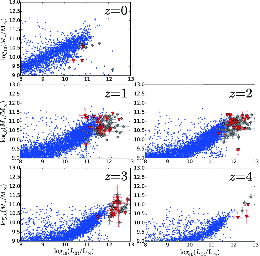
Figure 5: Relation between stellar mass and IR luminosity in the simulated galaxies (blue points) and the observational sample [gray diamonds ($\diamondsuit$; Lim et al., in preparation) and red triangles ($\triangledown$; Zavala et al. 2018)] at $z=0$, 1, 2, 3, and 4.

It is worth emphasizing the good match between the simulation and observation at the knees of luminosity functions. This is achieved by the depth of the STUDIES sample. However, we should keep in mind that it is still difficult to theoretically reproduce the brightest objects with $L_{\mathrm{IR}}\gtrsim 10^{13}$ L_☉. We discuss a possibility of explaining such luminous objects with AGN contribution in Section 5.4.

4.4 $T_{\rm dust}-L_{\rm IR}$ relation

In Fig. 7, we plot the $T_{\rm dust}$–$L_{\rm IR}$ relation at $z=1$–$4$ with observational results from STUDIES (Lim et al. in prep.) and Herschel (Casey et al., 2014). Because the observations only detect luminous objects $(L_{\rm IR}\gtrsim 10^{11}L_{\odot}~{}{\rm at}~{}z=1$ and $L_{\rm IR}\gtrsim 10^{12}L_{\odot}~{}{\rm at}~{}z=3)$, they can only be compared with the luminous population in our simulation. The dust temperatures of the luminous galaxies in our simulation are within the dispersion of the observed ones at all redshifts. The observational data seem to have greater dispersion than the theoretical predictions. The diversity in the small-scale dust distribution, which cannot be resolved in our simulation, could cause more dispersion in the dust temperature. Since a region with a higher dust temperature emit more, the inhomogeneity tends to raise the apparent $T_{\mathrm{dust}}$ (e.g. Sun & Hirashita, 2011) which could explain high-$T_{\mathrm{dust}}$ objects in the observational sample. We also find that the dust temperatures in the simulation tend to become higher as the redshift increases, which is not clearly seen in the observational sample that we are comparing against. However, we note that some observational studies showed that the dust temperatures tend to be higher at higher redshifts Schreiber et al. (2018).

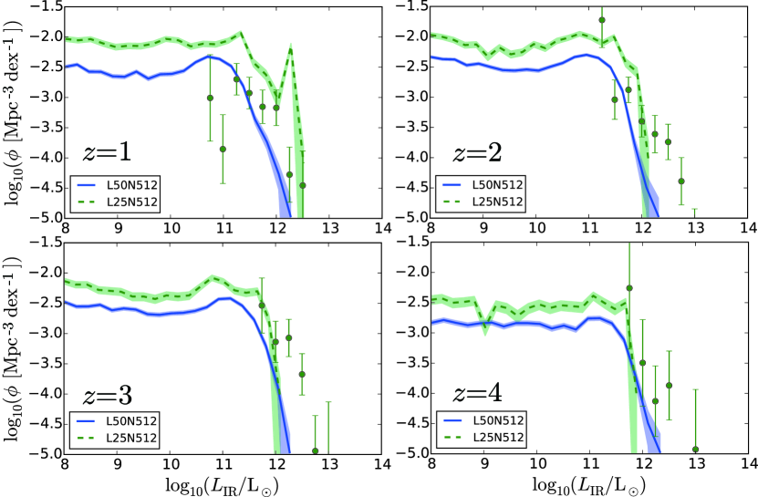
Figure 6: IR luminosity functions at $1\leq z\leq 4$. The solid blue and dashed green lines represent the results of L50N512 and L25N512, respectively. The shaded regions show the Poissonian error. The points with error bars are the STUDIES data.

In the simulation, we do not have sufficient number of galaxies with $L_{\mathrm{IR}}\gtrsim 10^{13}$ L_☉, but the extrapolation of the luminous end successfully explains the observed dust temperature. As we will discuss in Section 5.4, there could be an extra source of dust heating. Since the simulation box contains galaxies up to $L_{\mathrm{IR}}\sim 10^{12.5}$ L_☉, the increase of $L_{\mathrm{IR}}$ by a factor of 3 would be necessary. If we raise $L_{\mathrm{IR}}$ by a factor of 3, $T_{\mathrm{dust}}$ would be $3^{1/6}\simeq 1.2$ times higher (Eq. 17). Because the change in the dust temperature is small, the good match of $T_{\mathrm{dust}}$ between the simulation and observations is not significantly affected by the underestimate of $L_{\mathrm{IR}}$. Therefore, we conclude that the dust temperatures obtained in the simulation lie in a range consistent with the observed values.

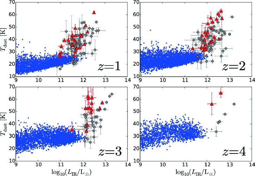
Figure 7: $T_{\rm dust}$-$L_{\rm IR}$ relation at $z=1$–4. The grey diamonds and red triangles with error bars are taken from the STUDIES sample (Lim et al., in preparation) and another SCUBA2 sample (Zavala et al., 2018), respectively.

4.5 IRX–$\beta_{\rm UV}$ relation

We show the IRX–$\beta_{\rm UV}$ relations at $z=1$–4 in Fig. 8. Because the IR-selected STUDIES sample is optically faint, the determination of $\beta_{\rm UV}$ is uncertain (i.e. error bars are large). Our simulation reproduces the observed IRX–$\beta_{\mathrm{UV}}$ relation in the following two aspects. First, the IRX values are broadly consistent with the observed ones. Since the observational sample is IR-selected, it only covers the high IRX values. Second, the $\beta_{\mathrm{UV}}$ values predicted by our simulation are roughly located in the middle of the observed range of $\beta_{\mathrm{UV}}$ for $z=1$–3, although the uncertainty in the observed $\beta_{\mathrm{UV}}$ is large. The sample size is too small at $z=4$.

Although it is difficult to derive an evolutionary trend from the scattered observational data, the theoretical results predict some evolutionary tendencies. As the redshift becomes higher, the extension of the simulation data toward large $\beta_{\mathrm{UV}}$ is less mainly because of less contribution from old stellar populations. The clump of data located between $\beta_{\mathrm{UV}}\sim-2$ and $-1$ is also seen at $z=0$ (Fig. 4), and is due to the optically thick limit of $\beta_{\rm UV}$ (see Appendix A). Although the observational error bars are large, there is a tension between theoretical and observational $\beta_{\mathrm{UV}}$ values in that the simulation underproduces galaxies with $\beta_{\mathrm{UV}}>0$. This may be partly resolved by changing the dust distribution geometry. As mentioned in Section 3.4, if we assume a screen geometry, $\beta_{\mathrm{UV}}$ can become larger; however, we should keep in mind that IRX also becomes larger (note that the observed IRX values are nicely reproduced by the simulation). Because of the large uncertainties in the observational $\beta_{\mathrm{UV}}$ values, we do not fine-tune the simulation results any further.

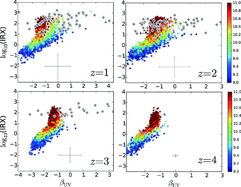
Figure 8: IRX–$\beta_{\rm UV}$ relation at $1\leq z\leq 4$. The colour bar indicates the logarithmic IR luminosity in units of ${\rm L}_{\odot}$ of each galaxy. The grey diamonds and black triangles show the observational samples (STUDIES data taken from Lim et al., in preparation and Herschel data from Casey et al. 2014). Note that Casey et al. (2014) took the average of $\beta_{\rm UV}$ for each IRX bin. The typical size of error bars for the STUDIES sample is shown in each panel.

5 Discussion

Although our simulation is successful in explaining some important aspects in the dust emission properties of the STUDIES sample, there are some discrepancies and uncertainties. In this section, we give further discussions on these issues.

5.1 Effect of spatial resolution

It is suggested that the brightness of a starburst is limited to $\lesssim 10^{13}$ L_⊙ kpc^-2 by radiation pressure (or the Eddington limit) (Crocker et al., 2018). Ideally, the simulation should be able to treat such a high-density starburst. However, in our simulation (or in cosmological simulations under the current computational resources), it is practically impossible to realize such an extreme starburst, as we estimate in what follows.

The highest gas density that can be achieved in the simulation is related to the smallest smoothing length of gas particles, $h_{\rm min}$. Since $h_{\rm min}\simeq 0.3$ kpc (physical) at $z=3$ for L50N512, only about 40 gas particles can be packed in a $\sim$1 kpc region. When we consider the situation that these gas particles with a mass of $7.0\times 10^{8}\,{\rm M}_{\odot}$ are converted into stars within a free-fall time of $\simeq 10^{7}$ yr, the intrinsic UV luminosity is estimated to be $2.5\times 10^{11}\,{\rm L}_{\odot}$ based on the population synthesis model we adopted. Therefore, if we consider that all UV photons are reprocessed into the IR by dust grains, the IR luminosity roughly corresponds to the cut-off scale of luminosity function in Fig. 6. In this sense, the lack of extremely IR-luminous objects could be due to the limited spatial resolution.

Indeed, as discussed in Section 4.3, a higher spatial resolution serves to produce luminous IR galaxies at $z=1$. However, a higher spatial resolution requires a smaller box size under a fixed computational resource. Since IR-luminous objects are rare, a large box size is also important. For example, if we halve the comoving box size to $12.5\,h^{-1}$ Mpc from $25\,h^{-1}$ Mpc, the objects with comoving number densities $\lesssim 10^{-3.5}$ Mpc^-3 cannot be produced, while the observations detect rare objects with $\sim 10^{-5}$ Mpc^-3. On the other hand, increasing the box size with a fixed particle number would reduce the resolution, and then the central region of IR-luminous objects such as compact starburst or AGN cannot be resolved. Ideally one would like to increase the box size and resolution at the same time with a larger number of particles; however, this requires far more computing resources, and it is not feasible at this moment.

Zoom-in simulations, which utilise higher resolution gas particles selectively in the region of interest, are a viable way of achieving a high resolution in cosmological simulations (e.g. Yajima et al., 2015; Hopkins et al., 2018). However, since the regions of interest are pre-selected, this method is not suitable for predicting statistical quantities such as luminosity function. On the other hand, it may be possible to apply a zoom-in method to one of the IR-brightest objects. This will enable us to test whether a dense gas concentration actually leads to an extremely IR-luminous objects or not.

5.2 Geometry of dust distribution

In the above, we assumed a mixed distribution of dust and stars. However, because there is an upper limit for $\beta_{\mathrm{UV}}$ as shown in Appendix A, $\beta_{\mathrm{UV}}$ could be underestimated in the mixed geometry. We could alternatively consider screen geometry, which does not have any upper limit for $\beta_{\mathrm{UV}}$. Totani & Takeuchi (2002) considered in their ‘screen model’ that only a part of dust is heated by stellar radiation. They explained the $T_{\mathrm{dust}}$–$L_{\mathrm{IR}}$ relation by the screen geometry rather than the ‘slab’ geometry. Our mixed geometry is close to their slab treatment. However, in our model, if we adopt the screen geometry, we find that some galaxies reach as high as IRX $\sim 10^{6}$. Since no observed galaxies show such a large value, the screen geometry is not suited for our purpose.

As mentioned above, a zoom-in simulation focusing on IR-luminous galaxies could resolve this issue, since we do not need to assume a specific relative distribution between dust and stars under a high enough spatial resolution. The highest zoom-in simulation today reach resolution of a few pc (e.g. FIRE-2 simulations by Hopkins et al., 2018), so the relative geometry of dust and gas can be resolved down to such scales if a dust model is implemented. Nevertheless, there could be even finer clumpy structure below a few pc, which warrants future research to clarify how such small-scale structures could play a role in the absorption and reemission by dust.

5.3 Variation of extinction curves

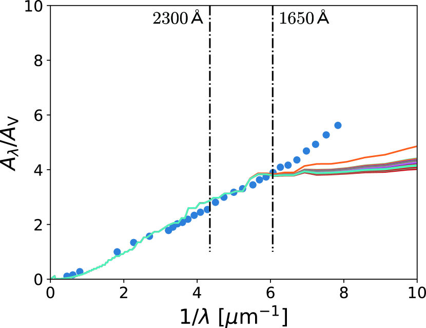
Figure 9: Extinction curves normalized to $A_{V}$ for galaxies with $L_{\mathrm{IR}}>10^{11}\,{\rm L}_{\odot}$ at $z=0$ (solid lines). The blue circles indicate the SMC extinction curve taken from Pei (1992). We mark the rest-frame wavelengths used to determine $\beta_{\mathrm{UV}}$ by the vertical dot-dashed lines (2300 Å on the left and 1650 Å on the right).

One of the new features of our dust treatment is that we included the grain size distribution in the form of the two-size approximation. Therefore, the extinction curve is a predicted quantity in our model. We show the extinction curves of IR-luminous galaxies in the simulation in Fig. 9. We only focus on galaxies with $L_{\mathrm{IR}}>10^{11}\,{\rm L}_{\odot}$ at $z=0$, which roughly corresponds to the luminosity range of the observational sample that we are comparing to. We normalize all extinction curves to $A_{V}$ (the extinction at $\lambda=0.55~{}\micron$) in order to focus on their shape. We also plot the SMC extinction curve taken from Pei (1992) in Fig. 9. The extinction curves in the simulation are consistent with the SMC curve at $\lambda>1650$ Å. At shorter wavelengths, the extinction is suppressed, which means that the grain abundance is dominated by large grains in those galaxies. This is due to efficient coagulation in the central parts of massive galaxies (see Aoyama et al., 2017; Hou et al., 2017). In our model, the value of $\beta_{\mathrm{UV}}$ is determined in the wavelength range where the extinction curve is approximated well by the SMC curve. In our separate work, Hou et al. (submitted) discuss the evolution of extinction curves. They showed that, if we focus on solar-metallicity ($Z\gtrsim 0.3$ Z_⊙) objects, which are valid for the IR-luminous objects in our simulation, the extinction curve does not evolve significantly over the redshift range. We confirmed that the extinction curves of IR-luminous objects do not change significantly along the redshift also in our simulation.

5.4 More dust heating by AGN and massive stars at high $z$?

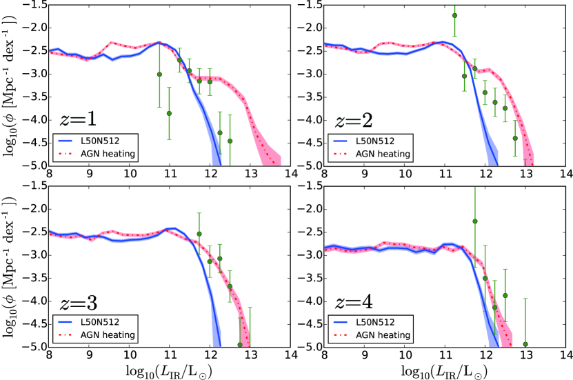
Figure 10: Possible impact of the extra dust heating by AGNs on the IR luminosity function at $z=1$–4. The red dotted and blue solid lines show the IR luminosity function with and without the AGN effect, respectively. The shaded region represent the 1-$\sigma$ uncertainty in Poisson statistics. The data points are the same as in Fig. 6.

In this paper, we only considered dust heating by stellar radiation. If AGNs contribute significantly to dust heating, the underproduction of the IR luminosity function could be explained by the lack of AGN treatment in our simulation. Gruppioni et al. (2013) estimated the fraction of AGN for galaxies ($0\leq z\leq 4$) detected by Herschel. After performing spectral analysis in a wide wavelength range ($0.1~{}\micron\leq\lambda\leq 1000~{}\micron$), they concluded that approximately 50 per cent of observed galaxies are classified as galaxies hosting an AGN. Chiang et al. (submitted) have shown that the number fraction of galaxies hosting an AGN is roughly 60 per cent for $L_{\mathrm{IR}}>10^{12}$ L_☉ and that the fraction does not change along redshift up to 2. On the other hand, the database of Chang et al. (2017) showed that approximately 10 per cent of galaxies have AGNs at the redshift range $2.0\leq z\leq 2.5$. Moreover, the contribution from AGNs is usually prominent at rest-frame mid-IR wavelengths according to the SED fitting by Chang et al. (2017); thus, it is not obvious if the above percentage reflects the fraction of AGNs contributing to the STUDIES bands. Recently, Toba et al. (2018) discovered an extremely IR-luminous galaxy ($L_{\mathrm{IR}}\sim 2\times 10^{14}$ L_☉) at $z=3.7$, in which a significant fraction of far-IR emission is contributed by an AGN, although the star formation has a comparable contribution to the AGN at wavelengths relevant for the STUDIES observations.

Although robust quantification of AGN contribution is still a matter of debate, we attempt the following extreme corrections in order to investigate the possible maximum contribution from AGNs to the total IR luminosity. We assume that a fraction super massive blackholes (SMBHs) manifest AGN activity and that the luminosity of the AGN is described by the Eddington luminosity of the SMBH. For simplicity, we also assume that all the radiation from the AGN is reprocessed into IR photons by surrounding dust grains.

The SMBH mass ($M_{\rm BH}$) can be estimated by the so-called Magorrian relation (Magorrian et al., 1998), and we calculate it according to Häring & Rix (2004) as

$$M_{\rm BH} = 10^{8.2}\left(\dfrac{M_{\rm bulge}}{10^{11}\,{\rm M}_{\odot}}\right)^{1.12}\,{\rm M}_{\odot}\,,$$ (20)

where $M_{\rm bulge}$ is the bulge mass of the galaxy. Since our simulation is not capable of resolving the galaxy morphology in detail, we simply use the total stellar mass for $M_{\mathrm{bulge}}$. The Eddington luminosity, $L_{\mathrm{Edd}}$ is estimated by (e.g. Rybicki & Lightman, 1979)

$$L_{\mathrm{Edd}} = \dfrac{4\pi GM_{\rm BH}m_{\rm p}c}{\sigma_{\rm T}}=5.07\times 10^{12}\left(\dfrac{M_{\rm bulge}}{10^{11}\,{\rm M}_{\odot}}\right)^{1.12}\,{\rm L}_{\odot}\,,$$

where $G$, $m_{\rm p}$ and $\sigma_{\rm T}$ are the gravitational constant, the mass of proton, and the Thomson scattering cross-section of electron, respectively. We add $L_{\mathrm{Edd}}$ to the IR luminosity which originates from the dust reprocessing of stellar light (equation 12) and regard the sum as the total IR luminosity for the galaxies which are chosen as AGN hosts.

We select galaxies hosting an AGN randomly with a probability given by the AGN fraction. The AGN fraction $f_{\rm AGN}$ is observationally investigated by Chiang et al. (submitted) in a wide redshift range of $0\leq z\leq 2.5$. They show that $f_{\rm AGN}$ is highly dependent on the IR luminosity and is almost independent of the redshift: $f_{\rm AGN}\simeq 0.6$ for $L_{\rm IR}\geq 10^{12}\,{\rm L}_{\odot}$, $f_{\rm AGN}\simeq 0.4$ for $10^{11}\,{\rm L}_{\odot}\leq L_{\rm IR}<10^{12}\,{\rm L}_{\odot}$ and $f_{\rm AGN}\simeq 0.1$ for $L_{\rm IR}<10^{11}\,{\rm M}_{\odot}$. We adopt the these $L_{\mathrm{IR}}$-dependent fractions, assuming that $f_{\mathrm{AGN}}$ does not depend on the redshift.

In Fig. 10, we show the IR luminosity functions with and without the AGN contribution. The extremely IR-luminous galaxies ($L_{\rm IR}\sim 10^{12.5}\,{\rm L}_{\odot}$) are well accounted for by the additional AGN contribution at $z>1$ in the L50N512 run. However, we overestimate the abundance of IR-luminous galaxies at $z=1$. Since A18’s simulation does not include AGN feedback, we probably need to include a consistent treatment between AGN feedback and emission in the future. Note again that our inclusion of AGN emission is based on an ‘extreme’ assumption that all the Eddington luminosity is reprocessed in the IR and that $M_{\mathrm{bulge}}$ is equal to the total stellar mass.

Another possible ‘extra’ heating could be due to a top-heavy IMF, which boosts the total stellar luminosity especially in the UV. Baugh et al. (2005) argued that their semi-analytic model, which is consistent with the Lyman-break galaxy luminosity function and the properties of the local galaxy population in the optical and IR, can explain the observed galaxy number counts at 850 $\mu$m only in the case of a top-heavy IMF. However, Hayward et al. (2013) used an empirical model based on simulations including galaxy–galaxy interactions, and suggested that the observed submm galaxy number counts do not provide evidence for a top-heavy IMF at high redshift. Zhang et al. (2018) have recently shown that the isotopic ratios of CO in massive starbursts support a top-heavy IMF. Because there is a large freedom in modeling a top-heavy IMF, we only mention that a top-heavy IMF is a possible way of reproducing the extremely IR-luminous objects.

6 Summary and Conclusions

We examine the consistency (and inconsistency) between the cosmological simulation with dust evolution and the deepest IR-selected observational sample. We choose the STUDIES sample for the observational data because of its depth and coverage at multiple wavelengths. We use the cosmological hydrodynamical simulation by A18, in which we computed the dust evolution consistently with the star formation activities and the local physical conditions of the ISM. We adopted the two-size approximation of grain size distribution (Hirashita, 2015), in which the entire grain radius range is represented by two sizes. In the simulation, we are able to trace spatial structures down to $\sim 1$ comoving kpc. For each galaxy identified in the simulation box, we calculate the dust optical depth, extinction curve (based on the grain size distribution), and intrinsic stellar SED. These quantities together with the dust mass enable us to estimate the IR luminosity, size of IR-emitting region, dust temperature, and observed stellar SED. We investigate the relations between the output quantities ($L_{\mathrm{IR}}$–$T_{\mathrm{dust}}$ and IRX–$\beta_{\mathrm{UV}}$ relations) as well as the IR LF.

First, we examine the radius of IR-emitting region for each galaxy in the simulation. We find that the radius $2R_{\mathrm{dust}}$ (where $R_{\mathrm{dust}}$ is the scale length of dust distribution) is consistent with interferometric observations of IR-luminous galaxies. Remarkably we also reproduce the evolution of IR-emitting radius toward $z=4$. Next, we test if our simulation reproduces the observed dust-emission properties by Herschel at $z=0$. We confirm that the IR LF, $L_{\mathrm{IR}}$–$T_{\mathrm{dust}}$ relation, and IRX–$\beta_{\mathrm{UV}}$ relation at $z=0$ are reproduced by our simulation.

Based on the model ‘calibrated’ by the above observational quantities, we compare our simulation results with the galaxy properties of the STUDIES sample at $z\sim 1$–4. We find that our simulation reproduces the $M_{*}$–$L_{\mathrm{IR}}$ relation, IR LFs (except at the luminous end $L_{\mathrm{IR}}\sim 10^{13}$ L_☉ at $z>2$), $T_{\mathrm{dust}}$–$L_{\mathrm{IR}}$ relation (except the large scatter seen in the observational sample), and the IRX–$\beta_{\mathrm{UV}}$ relation (except some high-$\beta_{\mathrm{UV}}$ objects in the observational sample). At $z\gtrsim 3$, we underproduce the extremely IR-luminous ($\gtrsim 10^{13}$ L_☉) objects even in the higher-resolution simulation. This is probably due to contributions from sources not included in our simulation such as AGNs. For the observed large scatter in the $T_{\mathrm{dust}}$–$L_{\mathrm{IR}}$ and IRX–$\beta_{\mathrm{UV}}$ relations, the variation of dust distribution geometry, which our simulation cannot resolve, could be a possible reason.

The broad success of our simulation indicates that the current dust evolution scenario is consistent with the observed galaxy properties in deep submm surveys. It means that the interstellar radiation field, which is roughly determined by the star formation history, is modelled self-consistently with the dust enrichment history in our cosmological hydrodynamic simulation. As for the extinction curve, the SMC-like extinction curve which is expected from our model is consistent with the IR-UV properties of the IR-luminous galaxies. In the future, we plan to extend our work using cosmological zoom-in simulations with higher resolution and address the issues that we discussed above.

Appendix A Stellar SED slope in mixed dust geometry

Here we discuss the behaviour of the IRX–$\beta_{\mathrm{UV}}$ relation in our model. If we describe the attenuation of stellar light as $\exp(-\tau_{\lambda})$, the observed luminosities at wavelengths $\lambda_{1}$ and $\lambda_{2}$ are estimated as

$$L_{\lambda_{1}} = \exp(-\tau_{\lambda_{1}})L_{\lambda_{1}}^{0}$$ (22)

$$L_{\lambda_{2}} = \exp(-\tau_{\lambda_{2}})L_{\lambda_{2}}^{0}=\exp(-\tau_{\lambda_{2}})L_{\lambda_{1}}^{0}\left(\dfrac{\lambda_{2}}{\lambda_{1}}\right)^{\beta_{\rm UV,int}},$$ (23)

where $\beta_{\rm UV,int}$ is intrinsic SED slope. In this case, $\beta_{\mathrm{UV}}$ is written based on Eq. (19) as

$$\beta_{\rm UV} = \dfrac{\left(\tau_{\lambda_{1}}-\tau_{\lambda_{2}}\right)\log_{10}(\mathrm{e})}{\log_{10}(\lambda_{2})-\log_{10}(\lambda_{1})}+\beta_{\rm UV,int}.$$ (24)

If we adopt the mixed geometry, the escape fraction at wavelength $\lambda$ is written as $f_{\rm esc}(\tau_{\lambda})=[1-\exp(-\tau_{\lambda})]/\tau_{\lambda}$. If we define the effective optical depth as

$$\tau_{{\rm eff,}\lambda}\equiv-\log_{\mathrm{e}}\left[\frac{1-\exp(-\tau_{\lambda})}{\tau_{\lambda}}\right],$$ (25)

we can use equation (24) by replacing $\tau_{\lambda}$ with $\tau_{\mathrm{eff},\lambda}$. In the optically thick limit, the effective optical depth becomes $\tau_{{\rm eff},\lambda}\to\log_{e}(\tau_{\lambda})$. By using this relation, we find that

$$\left(\beta_{\rm UV}-\beta_{\rm UV,int}\right)\to\dfrac{\log_{\mathrm{10}}(\tau_{\lambda_{1}}/\tau_{\lambda_{2}})}{\log_{10}(\lambda_{2}/\lambda_{1})}$$ (26)

for the optically thick limit ($\tau_{\lambda}\gg 1$). If we adopt the SMC extinction curve, which is appropriate for the massive galaxies in the simulation, using $\tau_{1650\AA}/\tau_{2500\AA}=1.712$ (Gordon et al., 2003), we obtain the following optically thick limit as

$$\left(\beta_{\rm UV}-\beta_{\rm UV,int}\right)\to 1.211.$$ (27)

Therefore, there is an upper limit for $\beta_{\rm UV}-\beta_{\rm UV,int}$ in the mixed geometry. For example, if $\beta_{\mathrm{UV,int}}=-2.5$, $\beta_{\mathrm{UV}}$ cannot exceed $-1.3$. In reality, because of contribution from old red stellar population, higher values of $\beta_{\mathrm{UV}}$ are also seen in the simulation.

References

- Amblard et al. (2010) Amblard A., et al., 2010, A&A, 518, L9
- Aoyama et al. (2017) Aoyama S., Hou K.-C., Shimizu I., Hirashita H., Todoroki K., Choi J.-H., Nagamine K., 2017, MNRAS, 466, 105
- Aoyama et al. (2018) Aoyama S., Hou K.-C., Hirashita H., Nagamine K., Shimizu I., 2018, Monthly Notices of the Royal Astronomical Society, 478, 4905
- Asano et al. (2014) Asano R. S., Takeuchi T. T., Hirashita H., Nozawa T., 2014, MNRAS, 440, 134
- Baugh et al. (2005) Baugh C. M., Lacey C. G., Frenk C. S., Granato G. L., Silva L., Bressan A., Benson A. J., Cole S., 2005, MNRAS, 356, 1191
- Bohren & Huffman (1983) Bohren C. F., Huffman D. R., 1983, Absorption and scattering of light by small particles. A Wiley-Interscience Publication
- Bouwens et al. (2014) Bouwens R. J., et al., 2014, ApJ, 793, 115
- Bouwens et al. (2016) Bouwens R. J., et al., 2016, ApJ, 833, 72
- Bruzual & Charlot (2003) Bruzual G., Charlot S., 2003, MNRAS, 344, 1000
- Burgarella et al. (2013) Burgarella D., et al., 2013, A&A, 554, A70
- Calanog et al. (2013) Calanog J. A., et al., 2013, ApJ, 775, 61
- Capak et al. (2015) Capak P. L., et al., 2015, Nature, 522, 455
- Casey et al. (2013) Casey C. M., et al., 2013, MNRAS, 436, 1919
- Casey et al. (2014) Casey C. M., et al., 2014, ApJ, 796, 95
- Chabrier (2003) Chabrier G., 2003, PASP, 115, 763
- Chang et al. (2017) Chang Y.-Y., et al., 2017, ApJS, 233, 19
- Chang et al. (2018) Chang Y.-Y., et al., 2018, ApJ,
- Clemens et al. (2013) Clemens M. S., et al., 2013, MNRAS, 433, 695
- Crocker et al. (2018) Crocker R. M., Krumholz M. R., Thompson T. A., Clutterbuck J., 2018, MNRAS, 478, 81
- Dayal et al. (2010) Dayal P., Hirashita H., Ferrara A., 2010, MNRAS, 403, 620
- Ferrara et al. (2017) Ferrara A., Hirashita H., Ouchi M., Fujimoto S., 2017, MNRAS, 471, 5018
- Finkelstein et al. (2012) Finkelstein S. L., et al., 2012, ApJ, 756, 164
- Fujimoto et al. (2017) Fujimoto S., Ouchi M., Shibuya T., Nagai H., 2017, ApJ, 850, 83
- Geach et al. (2013) Geach J. E., et al., 2013, MNRAS, 432, 53
- Geach et al. (2017) Geach J. E., et al., 2017, MNRAS, 465, 1789
- Gjergo et al. (2018) Gjergo E., Granato G. L., Murante G., Ragone-Figueroa C., Tornatore L., Borgani S., 2018, MNRAS, 479, 2588
- Gordon et al. (2003) Gordon K. D., Clayton G. C., Misselt K. A., Landolt A. U., Wolff M. J., 2003, ApJ, 594, 279
- Gruppioni et al. (2013) Gruppioni C., et al., 2013, MNRAS, 432, 23
- Hao et al. (2011) Hao C.-N., Kennicutt R. C., Johnson B. D., Calzetti D., Dale D. A., Moustakas J., 2011, ApJ, 741, 124
- Häring & Rix (2004) Häring N., Rix H.-W., 2004, ApJ, 604, L89
- Hayward et al. (2013) Hayward C. C., Narayanan D., Kereš D., Jonsson P., Hopkins P. F., Cox T. J., Hernquist L., 2013, MNRAS, 428, 2529
- Hirashita (2015) Hirashita H., 2015, MNRAS, 447, 2937
- Hopkins et al. (2018) Hopkins P. F., et al., 2018, MNRAS, 480, 800
- Hou et al. (2016) Hou K.-C., Hirashita H., Michałowski M. J., 2016, PASJ, 68, 94
- Hou et al. (2017) Hou K.-C., Hirashita H., Nagamine K., Aoyama S., Shimizu I., 2017, MNRAS, 469, 870
- Hwang & Geller (2013) Hwang H. S., Geller M. J., 2013, ApJ, 769, 116
- Kilerci Eser & Goto (2018) Kilerci Eser E., Goto T., 2018, MNRAS, 474, 5363
- Kong et al. (2004) Kong X., Charlot S., Brinchmann J., Fall S. M., 2004, MNRAS, 349, 769
- Koprowski et al. (2017) Koprowski M. P., Dunlop J. S., Michałowski M. J., Coppin K. E. K., Geach J. E., McLure R. J., Scott D., van der Werf P. P., 2017, MNRAS, 471, 4155
- Magnelli et al. (2013) Magnelli B., et al., 2013, A&A, 553, A132
- Magorrian et al. (1998) Magorrian J., et al., 1998, AJ, 115, 2285
- Mancini et al. (2016) Mancini M., Schneider R., Graziani L., Valiante R., Dayal P., Maio U., Ciardi B., 2016, MNRAS, 462, 3130
- McKinnon et al. (2017) McKinnon R., Torrey P., Vogelsberger M., Hayward C. C., Marinacci F., 2017, MNRAS, 468, 1505
- McKinnon et al. (2018) McKinnon R., Vogelsberger M., Torrey P., Marinacci F., Kannan R., 2018, MNRAS,
- Meurer et al. (1999) Meurer G. R., Heckman T. M., Calzetti D., 1999, ApJ, 521, 64
- Narayanan et al. (2018) Narayanan D., Davé R., Johnson B. D., Thompson R., Conroy C., Geach J., 2018, MNRAS, 474, 1718
- Pei (1992) Pei Y. C., 1992, ApJ, 395, 130
- Planck Collaboration et al. (2016) Planck Collaboration et al., 2016, A&A, 594, A13
- Popping et al. (2017a) Popping G., Somerville R. S., Galametz M., 2017a, MNRAS, 471, 3152
- Popping et al. (2017b) Popping G., Puglisi A., Norman C. A., 2017b, MNRAS, 472, 2315
- Reddy et al. (2012) Reddy N., et al., 2012, ApJ, 744, 154
- Rybicki & Lightman (1979) Rybicki G. B., Lightman A. P., 1979, Radiative processes in astrophysics. J. Wiley & Sons
- Saitoh (2017) Saitoh T. R., 2017, AJ, 153, 85
- Schreiber et al. (2018) Schreiber C., Elbaz D., Pannella M., Ciesla L., Wang T., Franco M., 2018, A&A, 609, A30
- Shimizu et al. (2012) Shimizu I., Yoshida N., Okamoto T., 2012, MNRAS, 427, 2866
- Smit et al. (2012) Smit R., Bouwens R. J., Franx M., Illingworth G. D., Labbé I., Oesch P. A., van Dokkum P. G., 2012, ApJ, 756, 14
- Springel (2005) Springel V., 2005, MNRAS, 364, 1105
- Springel et al. (2001) Springel V., White S. D. M., Tormen G., Kauffmann G., 2001, MNRAS, 328, 726
- Sun & Hirashita (2011) Sun A.-L., Hirashita H., 2011, MNRAS, 411, 1707
- Symeonidis et al. (2013) Symeonidis M., et al., 2013, MNRAS, 431, 2317
- Takeuchi et al. (2005) Takeuchi T. T., Buat V., Burgarella D., 2005, A&A, 440, L17
- Takeuchi et al. (2012) Takeuchi T. T., Yuan F.-T., Ikeyama A., Murata K. L., Inoue A. K., 2012, ApJ, 755, 144
- Toba et al. (2018) Toba Y., Ueda J., Lim C.-F., Wang W.-H., Nagao T., Chang Y.-Y., Saito T., Kawabe R., 2018, ApJ, 857, 31
- Totani & Takeuchi (2002) Totani T., Takeuchi T. T., 2002, ApJ, 570, 470
- Treyer et al. (2005) Treyer M., et al., 2005, ApJ, 619, L19
- Vlahakis et al. (2005) Vlahakis C., Dunne L., Eales S., 2005, MNRAS, 364, 1253
- Wang et al. (2017) Wang W.-H., et al., 2017, ApJ, 850, 37
- Weingartner & Draine (2001) Weingartner J. C., Draine B. T., 2001, ApJ, 548, 296
- Yajima et al. (2015) Yajima H., Shlosman I., Romano-Díaz E., Nagamine K., 2015, MNRAS, 451, 418
- Zavala et al. (2018) Zavala J. A., et al., 2018, MNRAS, 475, 5585
- Zhang et al. (2018) Zhang Z.-Y., Romano D., Ivison R. J., Papadopoulos P. P., Matteucci F., 2018, Nature, 558, 260