Analytic (3+1)-dimensional gauged Skyrmions, Heun and Whittaker-Hill equations and resurgence

Abstract

We show that one can reduce the coupled system of seven field equations of the (3+1)-dimensional gauged Skyrme model to the Heun equation (which, for suitable choices of the parameters, can be further reduced to the Whittaker-Hill equation) in two non-trivial topological sectors. Hence, one can get a complete analytic description of gauged solitons in (3+1) dimensions living within a finite volume in terms of classic results in the theory of differential equations and Kummer’s confluent functions. We consider here two types of gauged solitons: gauged Skyrmions and gauged time-crystals (namely, gauged solitons periodic in time, whose time-period is protected by a winding number). The dependence of the energy of the gauged Skyrmions on the Baryon charge can be determined explicitly. The theory of Kummer’s confluent functions leads to a quantization condition for the period of the time-crystals. Likewise, the theory of Sturm-Liouville operators gives rise to a quantization condition for the volume occupied by the gauged Skyrmions. The present analysis also discloses that resurgent techniques are very well suited to deal with the gauged Skyrme model as well. In particular, we discuss a very nice relation between the electromagnetic perturbations of the gauged Skyrmions and the Mathieu equation which allows to use many of the modern resurgence techniques to determine the behavior of the spectrum of these perturbations.

1 Introduction

In [1] it was shown that the low energy limit of QCD can be described by Skyrme theory [2]. The dynamical field of the Skyrme action is an $SU(N)$ valued scalar field (here we will consider the $SU(2)$ case) whose topological solitons (called Skyrmions) describe Baryons. In this context, the Baryon charge has to be identified with a suitable topological invariant (see [1], [3], [4], [5], [6], [7], [8], [9], [10] and references therein).

Hence, not surprisingly, the Skyrme model is very far from being integrable and, until very recently, no analytic solution with non-trivial topological properties was known. One of the problematic consequences of this fact is that the analysis of the phase diagram is quite difficult. In particular, analytic results on finite density effects and on the role of the Isospin chemical potential were unavailable despite the huge efforts in the pioneering references [11], [12], [13], [14], [15].

Even less is known on the (3+1)-dimensional gauged Skyrme model which describes the coupling of a $U(1)$ gauge field with the Skyrme theory. The importance, in many phenomenologically relevant situations, to analyze the interactions between Baryons, mesons and photons makes mandatory the task to arrive at a deeper understanding of the gauged Skyrme model (classic references are [1], [16] [17], [18], [19], [20]).

Obviously, the $U(1)$ gauged Skyrme model is “even less integrable” than the original Skyrme model. Consequently, as it was commonly assumed that to construct analytic gauged Skyrmions was a completely hopeless goal, mainly numerical tools were employed. Detailed numerical analysis of the gauged Skyrme model in non-trivial topological sectors can be found in [21], [22] and references therein.

Here it is worth to point out that to construct explicit topologically non-trivial solutions is not just of academic interest. First, such solutions allow to compute explicitly quantities of physical interest (such as the mass spectrum and the critical Isospin chemical potential). Secondly, once such solutions are available, one can test some modern ideas on how non-perturbative configurations can improve usual perturbation theory. We will come back on this issue in a moment.

Recently, in ([23], [24], [25], [26], [27], [28], [29], [30], [31] and references therein) new theoretical tools have been developed both in Skyrme and Yang-Mills theories (see [32], [33], [34] and references therein), which allow to build topologically non-trivial configurations even without spherical symmetry.

The first (3+1)-dimensional analytic and topologically non-trivial solutions of the Skyrme-Einstein system have been found in [28] using such tools. Skyrmions living within a finite box in flat space-times have been constructed using similar ideas in [35]: these results lead to the derivation of the critical isospin chemical potential beyond which the Skyrmion living in the box ceases to exist. Moreover, in the same reference, it has been shown for the first time that the Skyrme model admits Skyrmion-antiSkyrmion bound states. In [36], using the results in [28] and [35], a very efficient method to build analytic and topologically non-trivial solutions of the $U(1)$ gauged Skyrme model has been proposed: such a method will be exploited here.

There are two types of topologically non-trivial gauged solitons which can be obtained with the approach. The first type can be described as gauged Skyrmions living within a finite volume. The second type are smooth solutions of the $U(1)$ gauged Skyrme model whose periodic time-dependence is topologically protected (this type of solitons can be called topologically protected time-crystals).

Here we will show that both types of gauged solitons possess very special configurations which allow a complete analytic description (which, in the generic case, is not available) in terms of classic results in the theory of differential equations. In these two special cases it is possible to reduce the full system of seven coupled non-linear field equations of the gauged Skyrme model in non-trivial topological sectors to the Heun equation (which, in some cases, can be further reduced to the Whittaker-Hill equation). The only difference between the Heun equations appearing in the gauged Skyrmions and the gauged time-crystal sectors appears in the corresponding parameters. This remarkable mapping allows to argue, among other things, that the time period of the time-crystal is quantized (as it will be discussed in the following sections). Likewise, Sturm-Liouville theory gives rise to a quantization condition for the volume occupied by the gauged Skyrmions. Moreover, we will also show that a particular type of electromagnetic perturbations of these gauged solitons are described by the Mathieu equation (another very well analyzed equation in mathematical physics).

This brings another surprising outcome of the present construction. Namely resurgence does manifest itself in the (3+1)-dimensional gauged Skyrme model as well. Resurgence (very nice physically-oriented reviews are [37], [38], [39] and [40]) is currently the main framework which allows (at least in certain situations) to give a precise mathematical sense (using suitable non-perturbative informations) to the usual divergent perturbative expansions in quantum mechanics (QM) and quantum field theory (QFT).

As it is well known, most of the perturbative expansions appearing in theoretical physics are quite generically divergent. Resurgence helps in the following way. The proliferation of Feynman diagrams leads to a factorial growth of the perturbative coefficients and to the fact that the perturbative series is, at most, an asymptotic series. One can try Borel summation as a tool to give a meaning to such divergent series. However, in all the physically interesting situations analyzed so far, the initial divergent series becomes (through the Borel transform) a finite but ambiguous expression (these ambiguities manifest themselves along suitable lines in the complex $g$-plane, $g$ being the perturbative parameter). Obviously, this situation is unsatisfactory as well. However, when one analyzes theories with non-perturbative sectors one has to consider the perturbative expansions in each of these non-perturbative sectors too (as well as the fluctuations around them). It turns out that these non-perturbative contributions are also ambiguous in the Borel sense. Remarkably, as shown for the first time in the physical literature in [41] and [42] (as well as discussed in full generality in [43]), the non-perturbative ambiguities, at least in the models analyzed in that references, exactly cancel those of the perturbative sector. Hence, the perturbative divergence can be compensated by the non-perturbative sectors. This is, roughly speaking, the resurgent paradigm. Starting from the beautiful applications of resurgence techniques in [40], there has been a renewed interest on the applications of these ideas in theoretical physics. Most of the results have been obtained in integrable models, topological strings, QFT in 1+1 and 2+1 dimensions (in model such as N=2 SUSY Yang-Mills theory and the Principal Chiral models; see [44], [45] and references therein) and in many quantum mechanical problems (see [46], [47] and references therein). Two classic ordinary differential equations in which the resurgence paradigm works perfectly are the Mathieu and the Whittaker-Hill equations.

On the other hand, there have been very few explicit expressions of resurgence in non-integrable (3+1)-dimensional models. Thus, one may wonder whether the appearance of resurgent behavior is, in a sense, generic or it should be only expected in theories with a high degree of symmetries. The present results provide with strong evidence supporting the first hypothesis. Indeed, resurgence tools are very useful when analyzing the spectrum of electromagnetic perturbations of these gauged solitons.

This paper is organized as follows: In the second section, a short review of the gauged Skyrme model is presented. In the third section, gauged Skyrmions and time-crystals are introduced. In the fourth section, the relations between the Heun equation and the gauged solitons are explored. In Section 5, we draw some concluding ideas.

2 The $U(1)$ Gauged Skyrme Model

The action of the $U(1)$ gauged Skyrme model in four dimensions is

$$S =\int d^{4}x\sqrt{-g}\left[\frac{K}{2}\left(\frac{1}{2}\mathrm{Tr}\left(R^{\mu}R_{\mu}\right)+\frac{\lambda}{16}\mathrm{Tr}\left(G_{\mu\nu}G^{\mu\nu}\right)\right)-\frac{1}{4}F_{\mu\nu}F^{\mu\nu}\right]\ ,$$ (1)

$$R_{\mu} =U^{-1}D_{\mu}U\ ,\ \ G_{\mu\nu}=\left[R_{\mu},R_{\nu}\right]\ ,\ D_{\mu}=\nabla_{\mu}+A_{\mu}\left[t_{3},\ .\ \right]\ ,$$ (2)

$$U \in SU(2)\ ,\ \ R_{\mu}=R_{\mu}^{j}t_{j}\ ,\ \ t_{j}=i\sigma_{j}\ ,\ F_{\mu\nu}=\partial_{\mu}A_{\nu}-\partial_{\nu}A_{\mu}\ ,$$ (3)

where $g$ is the the metric determinant, $A_{\mu}$ is the gauge potential, $\nabla_{\mu}$ is the partial derivative, the positive parameters $K$ and $\lambda$ are fixed experimentally and $\sigma_{j}$ are the Pauli matrices. In our conventions $c=\hbar=\mu_{0}=1$, the space-time signature is $(-,+,+,+)$ and Greek indices run over space-time. The stress-energy tensor is

$$T_{\mu\nu}=-\frac{K}{2}\mathrm{Tr}\left[R_{\mu}R_{\nu}-\frac{1}{2}g_{\mu\nu}R^{\alpha}R_{\alpha}\right.\,+\left.\frac{\lambda}{4}\left(g^{\alpha\beta}G_{\mu\alpha}G_{\nu\beta}-\frac{g_{\mu\nu}}{4}G_{\sigma\rho}G^{\sigma\rho}\right)\right]+\bar{T}_{\mu\nu}\ ,$$

with

$$\bar{T}_{\mu\nu}=F_{\mu\alpha}F_{\nu}^{\;\alpha}-\frac{1}{4}F_{\alpha\beta}F^{\alpha\beta}g_{\mu\nu}\ ,$$ (4)

being the electromagnetic energy-momentum tensor. The field equations read

$$D^{\mu}\left(R_{\mu}+\frac{\lambda}{4}\left[R^{\nu},G_{\mu\nu}\right]\right)=0\ ,$$ (5)

$$\nabla_{\mu}F^{\mu\nu}=J^{\nu}\ ,$$ (6)

where $J^{\mu}$ is given by

$$J^{\mu}=\frac{K}{2}\text{Tr}\left[\widehat{O}R^{\mu}+\frac{\lambda}{4}\widehat{O}\left[R_{\nu},G^{\mu\nu}\right]\right]\ ,$$ (7)

with

$$\widehat{O}=U^{-1}t_{3}U-t_{3}\ .$$

It is worth to note that when the gauge potential reduces to a constant along the time-like direction, the field equations (5) describe the Skyrme model at a finite isospin chemical potential.

The term gauged Skyrmions and gauged time-crystals will refer to smooth regular solutions of the coupled system in Eqs. (5) and (6) possessing a non-vanishing winding number (defined below in Eq. (11)).

2.1 Gauged topological charge

The standard parametrization of the $SU(2)$-valued scalar $U(x^{\mu})$

$$U^{\pm 1}(x^{\mu})=Y^{0}(x^{\mu})\mathbb{\mathbf{I}}\pm Y^{i}(x^{\mu})t_{i}\ ,\ \ \left(Y^{0}\right)^{2}+Y^{i}Y_{i}=1\,,$$ (8)

where $\mathbb{\mathbf{I}}$ is the $2\times 2$ identity matrix and

$$Y^{0} =\cos C\ ,\quad Y^{i}=n^{i}\cdot\sin C\ ,$$ (9)

$$n^{1} =\sin F\cos G\ ,\ \ n^{2}=\sin F\sin G\ ,\ \ n^{3}=\cos F\ ,$$ (10)

will be useful in the following computations.

The expression for the topological charge for the gauged Skyrme model has been constructed in [16] (see also the pedagogical analysis in [21]):

$$W=\frac{1}{24\pi^{2}}\int_{\Sigma}\rho_{B}\ ,$$ (11)

where

$$\rho_{B}=\epsilon^{ijk}\text{Tr}\left\{\left(U^{-1}\partial_{i}U\right)\left(U^{-1}\partial_{j}U\right)\left(U^{-1}\partial_{k}U\right)-\partial_{i}\left[3A_{j}t_{3}\left(U^{-1}\partial_{k}U+\left(\partial_{k}U\right)U^{-1}\right)\right]\right\}\ .$$ (12)

There is an extra contribution with respect to the usual topological charge in the Skyrme model which is responsible for the so-called Callan-Witten effect [16].

The only case which is usually considered in the literature corresponds to a space-like $\Sigma$. In these situations $W$ is the Baryon charge of the configuration.

However, from the mathematical point of view, one can integrate the three-form $\rho_{B}$ on any three-dimensional hypersurface and, in any case, the number $W$ one obtains from Eq. (11) will be a topological invariant. In particular, in [35] and [36] it has been shown that very interesting configurations are obtained when $\Sigma$ is time-like (the light-like case is also worth to be further investigated). The interest of this case arises from the following considerations. First of all, when $W\neq 0$ (no matter which hypersurface one chooses) one cannot deform continuously the corresponding ansatz into $U=\mathbb{\mathbf{I}}$. Therefore, when $\rho_{B}$ is different from zero along a time-like hypersurface so that $\Sigma$ must be time-like in order to get $W\neq 0$ one gets non-trivial gauged solitons which depend on time (otherwise $\rho_{B}$ would vanish along time-like hypersurfaces). Moreover, the time-dependence of these gauged solitons is topologically protected since, by homotopy theory, $W$ cannot change under continuous deformations and this implies that they cannot decay into static configurations (since, for static configurations, $\rho_{B}$ vanishes along a time-like hypersurface). Since it turns out that these gauged solitons are periodic in time they can be called topologically protected time crystals. To the best of authors knowledge, the examples constructed in the following sections are the first time-periodic solutions whose time-period is topologically protected by homotopy theory. As it will be discussed in the following sections, classic results in the theory of Kummer’s confluent functions determine the allowed time-periods.

3 Gauged Skyrmions and Time Crystals

Here we will describe the theoretical tools introduced in [36], which are needed to build the novel gauged Skyrmions and the gauged time-crystals which will be analyzed in the following sections. Since one of the main physical motivations behind the analysis in [35], [36] was to study finite volume effects, the first step of the analysis is to put the gauged Skyrme model within a box of finite volume. The easiest way to achieve this goal is to introduce the following flat metric

$$ds^{2}=-dt^{2}+l^{2}\left(dr^{2}+d\gamma^{2}+d\phi^{2}\right)\ .$$ (13)

The length scale $l$ represents the size of the box. The dimensionless coordinates $r$, $\gamma$ and $\phi$ have the periods:

$$0\leq r\leq 2\pi\ ,\quad 0\leq\gamma\leq 4\pi\ ,\quad 0\leq\phi\leq 2\pi\ .$$ (14)

The following parametrization of the $SU(2)$-valued scalar $U$ will be considered:

$$U=e^{t_{3}\alpha}e^{t_{2}\beta}e^{t_{3}\rho}\ ,$$ (15)

where $\alpha$, $\beta$ and $\rho$ are the Euler angles which in a single covering of space take the values $\alpha\in[0,2\pi]$, $\beta\in[0,\frac{\pi}{2}]$ and $\rho\in[0,\pi]$.

3.1 Gauged Skyrmions

The ansatz for the gauged Skyrmion can be chosen as

$$\alpha=p\frac{\gamma}{2}\ ,\quad\beta=H(r)\ ,\quad\rho=q\frac{\phi}{2}\ ,\quad p,\ q\in\mathbb{N}\ .$$ (16)

In order for the ansatz to cover $SU(2)$ an integer number of times, the two parameters $p$ and $q\$ must be integer.

The profile $H$ must be static, and the electromagnetic potential has to be chosen as

$$A_{\mu}=(b_{1}(r),0,b_{2}(r),b_{3}(r))\ .$$ (17)

As it has been shown in [36], if one requires the following two conditions

$$X_{1}=-\frac{\lambda(p^{2}+q^{2})}{2}=\text{constant}\ ,$$ (18)

where

$$X_{1}(r):=4\lambda\left(-2l^{2}b_{1}^{2}+b_{2}(2b_{2}+p)+b_{3}(2b_{3}-q)\right)\ ,$$ (19)

and

$$b_{2}(r)=-\frac{q}{p}b_{3}(r)-\frac{p^{2}-q^{2}}{4p}\ ,$$ (20)

then the coupled Skyrme Maxwell system made by Eqs. (5) and (6) in a topologically non-trivial sector can be reduced consistently to the following system of two ODEs below

$$\left(\frac{8l^{2}}{p^{2}+q^{2}}+2\lambda\cos^{2}(H)\right)H^{\prime\prime}+\sin(2H)\left(l^{2}-\lambda H^{\prime 2}\right)=0\ ,$$ (21)

$$b_{3}^{\prime\prime}-\frac{K}{4}(q-4b_{3})\sin^{2}(H)\left(4l^{2}+4\lambda H^{\prime 2}+\lambda\left(p^{2}+q^{2}\right)\cos^{2}(H)\right)=0\ .$$ (22)

In other words, the three coupled gauged Skyrme equations in Eq. (5) and the corresponding four Maxwell equations in Eq. (6) with the Skyrme ansatz in Eqs. (15) and (16) and the gauge potential in Eq. (17) reduce to Eqs. (21) and (22) when the two algebraic conditions in Eqs. (18) and (20) are satisfied. This is a remarkable simplification and below we will show that indeed this sector contains physically relevant configurations.

Consequently, in order to construct explicitly gauged Skyrmions, the optimal strategy is to determine the Skyrme profile $H(r)$ from Eq. (21) and then, once $H(r)$ is known, Eq. (22) becomes a linear Schrodinger-like equation for the component $b_{3}(r)$ of gauge potential. Once $b_{3}$ is known, the other two components of the gauge potential are determined by the two algebraic relations in Eqs. (18) and (20).

It is worth to note that, generically, once Eq. (21) is solved in terms of suitable elliptic integrals, the resulting Eq. (22) (despite being a linear equation) will not have explicit analytic solutions. The reason is that the effective potential one gets replacing the solution of Eq. (21) into Eq. (22) will not be a solvable potential in the generic case.

In fact, in the following sections we will analyze the most elegant solutions of the above sector in which it is possible to obtain a complete analytic construction of gauged Skyrmions in terms of classic results in the theory of differential equations.

The Baryon number corresponding to the Skyrme ansatz in Eqs. (15) and (16) and to the gauge potential in Eq. (17) is

$$B=\int B_{0}drd\gamma d\phi=-p\,q\int\sin(2H)dH+2\Big{[}\cos^{2}(H(r))\left(q\,b_{2}(r)-p\,b_{3}(r)\right)\Big{]}_{0}^{2\pi},$$ (23)

and it leads to

$$B= -pq-2\left(q\,b_{2}(0)-p\,b_{3}(0)\right)=-\frac{(p^{2}+q^{2})(q-4b_{3}(0))}{2p}\ ,$$ (24a)

$$B= pq+2\left(q\,b_{2}(2\pi)-p\,b_{3}(2\pi)\right)=\frac{(p^{2}+q^{2})(q-4b_{3}(2\pi))}{2p}\ ,$$ (24b)

depending on the boundary values that we assume: $$H(2\pi)=\pi/2 H(0)=0 H(2\pi)=0 H(0)=\pi/2$$, or , respectively.

It is worth to point out that the gauged Skyrmions which will be constructed here are periodic in two spatial directions (namely $\gamma$ and $\phi$), while satisfy Dirichlet boundary condition in the coordinate $r$ (as it is clear from the fact that the values of $H(r)$ at $r=0$ and $r=\frac{\pi}{2}$ are fixed). Therefore, the spatial topology does not correspond to a $3$-torus but rather to a ($2$-torus)$\times$(finite interval), where the $2$-torus corresponds to the $\gamma$ and $\phi$ coordinates while the finite interval corresponds to the $r$ coordinate.

3.2 Gauged time crystal

Quite recently Wilczek and Shapere [48], [49], [50], asked the following very intriguing question (both in classical and in quantum physics): is it possible to spontaneously break time translation symmetry in physically sensible models?

These questions, until very recently, have been mainly analyzed in condensed matter physics. It is well known that powerful no-go theorems [51], [52] severely restrict the concrete realization of time-crystals. Novel versions of the original ideas (see [48], [49], [50]; a nice review is [53]) allowed to realize time-crystals in “solid-states” settings (see [54], [55], [56], [57], [58], [59] and references therein).

On the other hand, it seems that the first examples of time-periodic solutions which are topologically protected by homotopy theory in nuclear and particles physics have been found in [35], [36]. The key ingredients of the gauged Skyrme model is the possibility to have configurations with non-vanishing winding number along time-like hypersurfaces. Thanks to this fact, one can construct analytic time-periodic configurations which cannot be deformed continuously to the trivial vacuum as they possess a non-trivial winding number. Moreover, homotopy theory ensures that such solitons can only be deformed into other solitons with the same time period. Hence, these configurations can decay only into other time-periodic configurations. For these reasons, the name topologically protected time crystals is appropriate.

We will consider the line element in Eq. (13). The Skyrme ansatz in this case is

$$\alpha=\frac{\phi}{2}\ ,\quad\beta=H(r)\ ,\quad\rho=\frac{\omega t}{2}\ ,$$ (25)

where $\omega$ is a frequency so that $\rho$ is dimensionless (as it should be). One can see that, with the above ansatz, the topological density $\rho_{B}$ in Eq. (12) has a term proportional to

$$\rho_{B}\sim dt\wedge dr\wedge d\phi+...\ ,$$

where the dots represent terms which depend on $A_{\mu}$.

As far as the ansatz for the gauged-time crystal is concerned, it basically corresponds to a Wick rotation of the gauged Skyrmion in which one takes one of the two spatial periodic coordinates (which, for the gauged Skyrmions, are $\gamma$ and $\phi$) as time-like coordinate. Because of this, the dependence of the time-crystal on time is necessarily periodic. This explains why, in the case of the time-crystal, one can compute the winding number along the three-dimensional time-like hypersurface corresponding to the coordinates $t$, $\phi$ and $r$. The time-integration domain in the three-dimensional integral defining the winding number in the gauged time-crystal case corresponds to one period.

Thus, the above ansatz is a good candidate to be a time-crystal since its topological density can be integrated along a time-like hypersurface. The electromagnetic potential has the form (17), but the coordinate ordering is

$$x^{\mu}=(\gamma,r,t,\phi)\ .$$ (26)

In this case as well, as it has been shown in [36], if the following two relations among the three components of the gauge potential in Eq. (17)

$$X_{2}=\lambda\left(l^{2}\omega^{2}-1\right)=\text{constant}\ ,$$ (27)

where

$$X_{2}(r):=8\lambda\left(l^{2}b_{1}(\omega-2b_{1})+2b_{2}^{2}+b_{3}(1+2b_{3})\right)\ ,$$ (28)

and

$$b_{3}(r)=l^{2}\omega b_{1}(r)-\frac{l^{2}\omega^{2}}{4}-\frac{1}{4}\ ,$$ (29)

hold, then  the coupled Skyrme Maxwell system made by Eqs. (5) and (6) in a topologically non-trivial sector can be reduced consistently to the following system of two ODEs below:

$$2\left(\lambda\left(l^{2}\omega^{2}-1\right)\cos^{2}(H)-4l^{2}\right)H^{\prime\prime}+\left(l^{2}\omega^{2}-1\right)\sin(2H)\left(l^{2}-\lambda H^{\prime 2}\right)=0\ ,$$ (30)

$$b_{1}^{\prime\prime}+\frac{K}{8}(\omega-4b_{1})\sin^{2}(H)\left(l^{2}(\lambda\omega^{2}-8)-\lambda+\lambda\left(l^{2}\omega^{2}-1\right)\cos(2H)-8\lambda H^{\prime 2}\right)=0\ .$$ (31)

The optimal strategy is then to determine the Skyrme profile $H(r)$ from Eq. (30). Once $H(r)$ is known, Eq. (31) becomes a linear Schrodinger-like equation for the gauge potential component $b_{1}(r)$. The other components of the gauge potential are determined by solving the simple algebraic conditions in Eqs. (27) and (29).

Generically, once Eq. (30) is solved in terms of suitable elliptic integrals, the resulting Eq. (31) will not have explicit analytic solutions (despite being a linear equation). The reason is that the effective potential one gets replacing the solution of Eq. (30) into Eq. (31) will not be solvable.

In fact, in the following sections we will analyze the most elegant time-crystals in which it is possible to obtain a complete analytic construction in terms of classic results in the theory of differential equations.

As we did in the previous section for the gauged Skyrmion, we also calculate here for the time crystal the non vanishing winding number, that is

$$W=\int B_{2}drd\left(\omega\gamma\right)d\phi= 1+2\Big{[}\cos^{2}(H(r))\left(\frac{b_{1}(r)}{\omega}-b_{3}(r)\right)\Big{]}_{0}^{2\pi}$$

$$= 1-2\left(\frac{b_{1}(0)}{\omega}-b_{3}(0)\right)$$

$$= \frac{(1-l^{2}\omega^{2})\left(\omega-4b_{1}(0)\right)}{2\omega}\ ,$$ (32)

if we consider $r\in[0,2\pi]$, $\omega\gamma\in[0,4\pi]$, $\phi\in[0,2\pi]$ and $H(2\pi)=\pi/2$, $H(0)=0$.

However, a normal topological charge is also present here due to the correction from the electromagnetic potential. By taking $B_{0}$ as defined in (12) as an integral over spatial slices, we obtain

$$B=\int B_{0}drdzd\phi=-2\Big{[}\cos^{2}(H(r))b_{2}(r)\Big{]}_{0}^{2\pi}=2b_{2}(0)=\frac{l}{2}(\omega-4b_{1}(0))\sqrt{1-l^{2}\omega^{2}}\ ,$$

with the same boundary values used as in (32), with the difference now that we have $z$ in place of $\gamma$ for which we consider $z\in[0,2\pi]$. The charge $B$ is non zero as long as $b_{2}(0)\neq 0$.

In the following sections we will analyze the most elegant solutions of the above sector.

3.3 Extended duality

In this subsection it is shown that a sort of electromagnetic duality exists between the gauged Skyrmion and the gauged time-crystal constructed above. In order to achieve this goal, it is useful to observe that a mapping between the time crystal to the Skyrmion should involve a transformation

$$\gamma\rightarrow i\,l\,\gamma\ ,\qquad z\rightarrow\frac{i}{l}z\ ,$$ (33)

so that the signature can be changed appropriately. Then, it is an easy task to see that Eq. (30) and Eq. (31) are mapped to Eq. (21) and Eq. (22) under the linear transformation

$$a_{1}=\frac{i}{l}b_{2}\ ,\quad a_{2}=i\,l\,b_{1}\ ,\quad a_{3}=-b_{3}\ .$$ (34)

The appearance of the imaginary units is not alarming, since one also needs a coordinate transformation like (33) to map the one space-time metric to the other. Notice that the imaginary part of the transformation involves only the $\gamma$ and $z$ components of $A_{\mu}$. Hence, the end result after utilizing (33) is a real electromagnetic tensor of the Skyrmion case.

In the following two tables we gather the electromagnetic potentials of the Skyrmion and of the time crystal (T.C.) as well the necessary transformations that need to be made - not only to the field but also to parameters and variables - in order to make the transition from the one case to the other.

$$A_{\mu}$$ coordinate system time variable

Skyrmion

T. C. before transformation

         T.C.     $$\longrightarrow$$    Skyrmion

4 Heun equation and gauged solitons

Here it will be discussed how the Heun and Whittaker-Hill equations appear in the construction of both gauged Skyrmions and gauged time-crystals described above. In the first subsection we will analyze the gauged Skyrmions and in the second subsection the gauged time-crystals will be considered. In both subsections, we will use following simple generalization of the metric (13)

$$ds^{2}=-dt^{2}+l_{1}^{2}dr^{2}+l_{2}^{2}d\theta^{2}+l_{3}^{2}d\phi^{2}\ ,$$ (35)

corresponding to a box with sides with different sizes while the periods of the coordinates will be the same as in Eq. (14). The reduction of the coupled gauged Skyrme and Maxwell field equations obtained in [36] also holds with the above metric.

It is a quite remarkable feature of the present gauged solitons that, in both families, one can give a complete analytical description of these (3+1)-dimensional topological objects in a theory (the gauged Skyrme model), which is far from being integrable, in terms of the solutions of the Heun and Whittaker-Hill equations (which are well-known example of quasi-integrable equations [60], [61]). Besides the intrinsic interest of this result, the present framework clearly shows that the resurgence paradigm is also very effective in the low energy limit of QCD coupled to electrodynamics. In particular, electromagnetic perturbations of the gauged Skyrmions satisfy the Mathieu equation which is very well suited for the resurgence approach in [45], [46], [47].

In view of the results of [45], the present results disclose an unexpected relation between the (3+1)-dimensional gauged Skyrme model and the so-called $\eta$-deformed Principal Chiral Models.

4.1 Heun equation and gauged Skyrmions

A direct computation shows that, using the line element in Eq. (35), the three coupled gauged Skyrme equations (namely, $\mathit{E}^{j}=0$, $j=1$, $2$, $3$) in Eq. (5)

$$D^{\mu}\left(R_{\mu}+\frac{\lambda}{4}\left[R^{\nu},G_{\mu\nu}\right]\right)=\mathit{E}^{j}t_{j}=0$$

and the corresponding four Maxwell equations in Eq. (6) are greatly simplified by the Skyrme ansatz in Eqs. (15) and (25) and the gauge potential in Eq. (17).

Indeed, Eq. (5) reduce to only one Skyrme field equation (since the third Skyrme equation is identically satisfied while the first and the second are proportional):

$$\mathit{E}^{3} = 0\ ,$$

$$\mathit{E}^{1} = I_{1}P\left[H\right]\ ,\ \mathit{E}^{2}=I_{2}P\left[H\right]\ ,\ \ I_{1}\neq 0\ ,\ I_{2}\neq 0\ ,$$

where $I_{j}$ are real and non-vanishing, while

$$0 =P\left[H\right]=4\left(X_{1}\sin^{2}(H)+\frac{\lambda l_{1}^{2}}{2}\left(\frac{p^{2}}{l_{2}^{2}}+\frac{q^{2}}{l_{3}^{2}}\right)+2l_{1}^{2}\right)H^{\prime\prime}+2X_{1}\sin(2H)H^{\prime 2}+4\sin^{2}(H)X_{1}^{\prime}H^{\prime}$$

$$+\left(2\lambda l_{1}^{4}\left(\frac{pb_{2}}{l_{2}^{2}}+\frac{qb_{3}}{l_{3}^{2}}\right)\left(\frac{pb_{2}}{l_{2}^{2}}+\frac{qb_{3}}{l_{3}^{2}}+\frac{1}{2}\left(\frac{p^{2}}{l_{2}^{2}}-\frac{q^{2}}{l_{3}^{2}}\right)\right)-\frac{l_{1}^{4}}{l_{2}^{2}l_{3}^{2}}\frac{\lambda p^{2}q^{2}}{2}-\frac{l_{1}^{2}}{4}\left(\frac{p^{2}}{l_{2}^{2}}+\frac{q^{2}}{l_{3}^{2}}\right)X_{1}\right)\sin(4H)$$

$$-\frac{2l_{1}^{2}}{\lambda}X_{1}\sin(2H)\ ,$$

where

$$X_{1}=4\lambda\left(-2l_{1}^{2}b_{1}^{2}+\frac{l_{1}^{2}}{l_{2}^{2}}b_{2}(2b_{2}+p)+\frac{l_{1}^{2}}{l_{3}^{2}}b_{3}(2b_{3}-q)\right)\ .$$

On the other hand, the Maxwell equations reduce to

$$b_{I}^{\prime\prime}=-\frac{K}{2}\left(M_{IJ}b_{J}+N_{I}\right)\ ,$$

with

$$M_{11} =4\sin^{2}(H)\left(2\lambda H^{\prime 2}+\frac{\lambda l_{1}^{2}}{2}\left(\frac{p^{2}}{l_{2}^{2}}+\frac{q^{2}}{l_{3}^{2}}\right)\cos^{2}(H)+2l_{1}^{2}\right)\ ,\qquad M_{23}=-\frac{l_{1}^{2}}{2l_{3}^{2}}\lambda pq\sin^{2}(2H)\ ,$$

$$M_{22} =M_{11}+\frac{p}{q}M_{32}\ ,\qquad M_{32}=\frac{l_{3}^{2}}{l_{2}^{2}}M_{23}\ ,\qquad M_{33}=M_{11}+\frac{q}{p}M_{23}\ ,\qquad N_{1}=0\ ,$$

$$N_{2} =\frac{p}{4}M_{11}+\frac{1}{4q}\left(\frac{l_{3}^{2}p^{2}}{l_{2}^{2}}-q^{2}\right)M_{23}\ ,\qquad N_{3}=-\frac{q}{4}M_{11}+\frac{1}{4p}\left(\frac{l_{3}^{2}p^{2}}{l_{2}^{2}}-q^{2}\right)M_{23}\ .$$

Once again, when algebraic relations below hold

$$X_{1}=-\frac{\lambda l_{1}^{2}}{2}\Big{(}\frac{p^{2}}{l_{2}^{2}}+\frac{q^{2}}{l_{3}^{2}}\Big{)}=\text{constant}\ ,\qquad\frac{p}{l_{2}^{2}}b_{2}+\frac{q}{l_{3}^{2}}b_{3}=-\frac{1}{4}\Big{(}\frac{p^{2}}{l_{2}^{2}}-\frac{q^{2}}{l_{3}^{2}}\Big{)}\ ,$$ (36)

the system of seven coupled non-linear field equations of the gauged Skyrme model reduce to

$$\Big{(}8\big{(}\frac{p^{2}}{l_{2}^{2}}+\frac{q^{2}}{l_{3}^{2}}\big{)}^{-1}+2\lambda\cos^{2}(H)\Big{)}H^{\prime\prime}+\sin(2H)(l_{1}^{2}-\lambda H^{\prime 2})=0\ ,$$ (37)

$$b_{3}^{\prime\prime}-\frac{K}{4}(q-4b_{3})\sin^{2}(H)\Big{\{}4l_{1}^{2}+4\lambda H^{\prime 2}+\lambda l_{1}^{2}\big{(}\frac{p^{2}}{l_{2}^{2}}+\frac{q^{2}}{l_{3}^{2}}\big{)}\cos^{2}(H)\Big{\}}=0\ .$$ (38)

The above system is a slight generalization of the one obtained in [36].

The simplest topologically non-trivial solution for the profile $H(r)$ is given by

$$H(r)=\frac{l_{1}}{\sqrt{\lambda}}r+h_{0}\ ,$$ (39)

where $h_{0}$ is a constant. It is important to satisfy the necessary conditions needed to have a non-vanishing topological charge:

$$H(2\pi)=\pi/2,\ H(0)=0\ ,\qquad\text{or}\qquad H(2\pi)=0,\ H(0)=\pi/2\ .$$

The above conditions fix $l_{1}$ and $h_{0}$ as follows:

$$l_{1}=\frac{\sqrt{\lambda}}{4}\ ,\ h_{0}=0\ ,\qquad\text{or}\qquad l_{1}=-\frac{\sqrt{\lambda}}{4}\ ,\ h_{0}=\frac{\pi}{2}\ .$$ (40)

Moreover, the energy density of the system is found to be

$$\varepsilon =\frac{K}{2}\left[\frac{1}{\lambda}+\frac{1}{2}\left(\frac{p^{2}}{l_{2}^{2}}+\frac{q^{2}}{l_{3}^{2}}\right)+\left(\frac{1}{\lambda l_{1}^{2}}X_{1}+16b_{1}^{2}\right)\sin{H}^{2}+\frac{\lambda}{4}\left(b_{1}^{2}\left(\frac{p^{2}}{l_{2}^{2}}+\frac{q^{2}}{l_{3}^{2}}\right)+\frac{1}{4l_{2}^{2}l_{3}^{2}}\left(2qb_{2}-2pb_{3}+pq\right)^{2}\right)\sin{(2H)}^{2}\right]$$

$$\qquad+\frac{1}{2l_{1}^{2}}\left(b_{1}^{\prime 2}+\frac{b_{2}^{\prime 2}}{l_{2}^{2}}+\frac{b_{3}^{\prime 2}}{l_{3}^{2}}\right)\ .$$ (41)

The above expression will be discussed in more details after constructing the complete solution of the problem in terms of the Heun functions.

In what follows, we will study the equation (38). By introducing the new variables $x$ and $y$ given by

$$x=\frac{l_{1}}{\sqrt{\lambda}}r+h_{0}\ ,\qquad y=q-4b_{3}\ ,$$ (42)

we can rewrite the equation (38) as

$$\frac{d^{2}y}{dx^{2}}+\Big{(}8K\lambda\ \sin^{2}x+\Gamma^{2}\sin^{2}2x\Big{)}y=0\ ,$$ (43)

with a non-negative constant $\Gamma\geq 0$,

$$\Gamma^{2}:=\frac{K\lambda^{2}}{4}\Big{(}\frac{p^{2}}{l_{2}^{2}}+\frac{q^{2}}{l_{3}^{2}}\Big{)}\ .$$

The equation (43) can be cast into the famous confluent Heun’s equation,

$$\frac{d^{2}}{dz^{2}}Y(z)+\Big{(}\frac{\gamma}{z}+\frac{\delta}{z-1}+\epsilon\Big{)}\frac{d}{dz}Y(z)+\frac{\alpha z-q}{z(z-1)}Y(z)=0\$$ (44)

where

$$z=\cos^{2}x\ ,\qquad Y(z)=e^{-i\Gamma z}\ y(\arccos\sqrt{z})\ ,$$

$$\gamma=\delta=1/2\ ,\qquad\epsilon=2i\Gamma\ ,\qquad\alpha=i\Gamma+2K\lambda\ ,\qquad q=i\Gamma/2+2K\lambda\ .$$ (45)

A general solution to this equation is found to be

$$Y(z)=C_{1}\ \text{HeunC}(i\Gamma+2K\lambda,1/2,1/2,2i\Gamma,i\Gamma/2+2K\lambda;z)$$

$$\hskip 36.135pt+C_{2}\sqrt{z}\ \text{HeunC}(2i\Gamma+2K\lambda,3/2,1/2,2i\Gamma,3i\Gamma/2+2K\lambda-1/4;z)\ ,$$ (46)

where $C_{1}$ and $C_{2}$ are integration constants, and $\text{HeunC}(\alpha,\gamma,\delta,\epsilon,q;z)$ is the confluent Heun’s function.

4.1.1 Electric field, magnetic field and boundary conditions

The non-zero components of the electromagnetic tensor in our configuration are given by

$$E_{r}=\frac{\sqrt{l_{3}^{2}p^{2}+l_{2}^{2}q^{2}}}{l_{3}^{2}p}b_{3}^{\prime}\ ,\quad B_{\theta}=\frac{1}{l_{1}^{2}l_{3}^{2}}b_{3}^{\prime}\ ,\quad B_{\phi}=\frac{q}{l_{1}^{2}l_{3}^{2}p}b_{3}^{\prime}\ .$$

The requeriment that the electric field on the surface of the box ($r=0$ and $r=2\pi$) vanishes leads to $b_{3}^{\prime}(0)=b_{3}^{\prime}(2\pi)=0$. Since in Eq. (38) the unknown is $b_{3}(r)$, imposing a condition on the electric and magnetic field induces Neumann boundary conditions for this potential (note also that since $b_{3}$ is part of a gauge conection, it is defined up to an additive constant). Notwithstanding Eq. (38) can be solved analytically in terms of Confluent Heun functions, it is simpler to impose the boundary condition in a numerical integration. Then Eq. (43) defines the following Sturm-Liouville problem

$$\frac{d}{dx}\left(\hat{p}\left(x\right)\frac{d}{dx}y\left(x\right)\right)+\hat{Q}\left(x\right)y\left(x\right)=-\Gamma^{2}\hat{w}\left(x\right)y\left(x\right)\ ,$$ (47)

where

$$\hat{w}\left(x\right) = \sin^{2}2x\ ,\ \ \hat{p}\left(x\right)=1$$

$$\hat{Q}\left(x\right) = 8K\lambda\sin^{2}x\ .$$

Since $\Gamma^{2}$ plays the role of the eigenvalue of the Sturm-Liouville problem defined above, then there is a countable infinity of values for $\Gamma$ which are consistent with the boundary conditions imposed. Since $p$ and $q$ are integers, the quantization of $\Gamma$ induces a quantization on the possible values of the volume within which the gauged baryons are confined!

Figure 1 shows the profiles for $b_{3}^{\prime}$ for the first five allowed values of $\Gamma$. The non-triviality of the profile inside the box is due to the presence of the current.

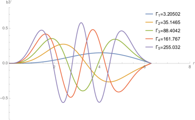
Figure 1: Behaviour of $b_{3}^{\prime}(r)$ for the first values of $\Gamma$.

4.1.2 Gauged Skyrmion energy

In order to do the energy plots it is enough to consider the case in which

$$p=q\ ,\ \quad l_{2}=l_{3}\ ,$$

so that the Baryon charge is

$$B=p^{2}=q^{2}\ ,$$

while the area $\widetilde{A}$ of the box orthogonal to the $r$-axis is

$$A=\frac{\widetilde{A}}{8\pi^{2}}=l_{2}^{2}=l_{3}^{2}\ .$$

On the other hand, the total volume is

$$V=2\pi l_{1}\widetilde{A}=32\pi^{3}\frac{\sqrt{\lambda}}{4}l_{2}^{2}\ .$$

Thus, the energy density of the system reads

$$\varepsilon= \frac{K}{2}\left[\frac{1}{\lambda}+\frac{B}{A}+\left(\frac{1}{\lambda l_{1}^{2}}X_{1}+16b_{1}^{2}\right)\sin{H}^{2}+\frac{\lambda}{4}\left(2\frac{B}{A}b_{1}^{2}+\frac{1}{4A^{2}}\left(2B^{1/2}b_{2}-2B^{1/2}b_{3}+B\right)^{2}\right)\sin{(2H)}^{2}\right]$$

$$+\frac{1}{2l_{1}^{2}}\left(b_{1}^{\prime 2}+\frac{b_{2}^{\prime 2}+b_{3}^{\prime 2}}{A}\right)$$

$$= \frac{K}{32A^{2}\lambda}(16A^{2}+24AB\lambda+B^{2}\lambda^{2}-B\lambda(8A\cos(2H)+B\lambda\cos(4H))$$

$$-32K\lambda(B^{1/2}-2b_{3})b_{3}(8A+B\lambda\cos(2H))\sin^{2}(H)+256Ab_{3}^{\prime 2})\ .$$ (48)

Figure 2 show the energy as function of the area. The divergence for low values of the area is expected on general ground since, at very small distances, the Skyrme model should be replaced by QCD.

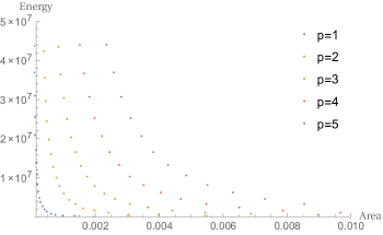
Figure 2: Energy of the system as a function of the area for $p=1,2,3,4,5$.

4.1.3 Relation with the Whittaker-Hill equation

If we take a coordinate transform

$$y=q-4b_{3}\ ,\qquad x=\frac{l_{1}}{\sqrt{\lambda}}r+h_{0}\ ,$$ (49)

and use the equation (39) in (38), then we have a Whittaker-Hill equation

$$\frac{d^{2}y}{dx^{2}}+\left(4\alpha s\cos(2x)+2\alpha^{2}\cos(4x)+\lambda_{0}\right)y=0\ ,$$ (50)

where

$$\alpha^{2} = -\frac{K\lambda^{2}}{16}\Big{(}\frac{p^{2}}{l_{2}^{2}}+\frac{q^{2}}{l_{3}^{2}}\Big{)}\ ,\qquad s=4i\Big{(}\frac{p^{2}}{Kl_{2}^{2}}+\frac{q^{2}}{Kl_{3}^{2}}\Big{)}^{-1/2}\ ,$$ (51)

$$\qquad\lambda_{0} = K\lambda\Big{\{}4+\frac{\lambda}{8}\Big{(}\frac{p^{2}}{l_{2}^{2}}+\frac{q^{2}}{l_{3}^{2}}\Big{)}\Big{\}}\ ,$$ (52)

and $\lambda_{0}$ is an eigenvalue of the differential operator. It is not true, however, that the Heun equation discussed in the previous subsection is equivalent to the Whittaker-Hill equation (indeed, the relation of the present gauged solitons with the Heun equation is more natural), because the parameters $\alpha$ and $s$ are not independent (unlike what would happen in a “proper” Whittaker-Hill equation). Thus, $s$ need not be an integer. Indeed,

$$\alpha=-K\lambda/s\ ,\qquad\lambda_{0}=4K\lambda-2K^{2}\lambda^{2}/s^{2}\ .$$ (53)

Now, we can compare Eq. (50) with the Whittaker-Hill’s equation in [45],

$$\psi^{\prime\prime}+(a-2b\cos 2x-2c\cos 4x)\psi=0\ ,$$ (54)

where

$$a=\lambda_{0}\ ,\qquad b=-2\alpha s\ ,\qquad c=-\alpha^{2}\ .$$ (55)

From their analysis we can obtained the resurgent parameter of our model, that is

$$g^{2}=\frac{1}{2\sqrt{4\alpha^{2}+2\alpha s}}=\frac{il_{2}l_{3}}{\sqrt{K\lambda\left(\lambda l_{2}^{2}q^{2}+\lambda l_{3}^{2}p^{2}+8l_{2}^{2}l_{3}^{2}\right)}}\ .$$ (56)

4.1.4 Perturbations, Mathieu equation and resurgence

In this subsection we will discuss how typical electromagnetic perturbations of the gauged Skyrmions constructed above disclose the resurgence structure of these (3+1)-dimensional gauged solitons. Before entering into the technical details, it is worth to remind how standard large N arguments can simplify the analysis of the present subsection (see for a detailed review chapter 4-in particular, section 4.2-of the classic reference [5]). As it is well known, in the leading ’t Hooft approximation, in meson-Baryon scattering, the very heavy Baryon (the Skyrmion in our case) is essentially unaffected and, basically, only the meson can react. This is even more so in the photon-Baryon semiclassical interactions (due to the masslessness of the photon). Thus, in this approximation, electromagnetic perturbations perceive the Skyrmions as an effective medium. From the practical point of view, this simplifies the analysis since one can neglect the perturbations of the Skyrmions (suppressed by powers of 1/N) and one is allowed to only consider the reaction of the Maxwell equations to perturbations around the gauged Skyrmion background. In other words, one can consider electromagnetic perturbations of Eqs. (6) and (7) in which the background solution is the gauged Skyrmion defined in Eqs. (16), (17), (35), (36), (39) and (40).

As it is well known, the full power of resurgence manifests itself especially in relating the perturbative expansion around the trivial vacuum with the perturbative expansions around non-trivial saddles. In the present case, the analysis of the full perturbative expansion around the gauged solitons constructed in the previous sections would correspond to the analysis of seven coupled linear PDEs in the background of gauged solitons discussed above. This analysis is extremely difficult even numerically. Consequently, we considered a simpler (yet interesting) situation in which the Skyrme background is considered to be fixed and one analyzes magnetic perturbations of the Maxwell equations in the background of the gauged Skyrmion itself (this situation is enough to show that resurgence appears also in the gauged Skyrme model).

Thus, let’s consider the following perturbations around the solutions defined in Eqs. (16), (17), (36), (39) and (40):

$$b_{2}(r)\rightarrow b_{2}(r)+\epsilon c_{2}(r)\sin(\Omega t)\ ,\quad b_{3}(r)\rightarrow b_{3}(r)+\epsilon c_{3}(r)\sin(\Omega t)\ ,$$ (57)

$\Omega$ being the frequency of the perturbation: the mathematical problem is to find how $\Omega$ depends on the parameters of the problem. To first order in $\epsilon$, Eqs. (6) and (7) reduce to

$$0\quad=\quad 4l_{3}^{2}c_{2}^{\prime\prime}(r)-Kl_{1}^{2}pq\lambda c_{3}(r)\sin^{2}(2H)$$

$$+\frac{1}{2}l_{1}^{2}c_{2}(r)\left(32Kl_{3}^{2}+Kq^{2}\lambda+8l_{3}^{2}\Omega^{2}-32Kl_{3}^{2}\cos(2H)-Kq^{2}\lambda\cos(4H)\right)\ ,$$ (58)

$$0\quad=\quad 4l_{2}^{2}c_{3}^{\prime\prime}(r)-Kl_{1}^{2}pq\lambda c_{2}(r)\sin^{2}(2H)$$

$$+\frac{1}{2}l_{1}^{2}c_{3}(r)\left(32Kl_{2}^{2}+Kp^{2}\lambda+8l_{2}^{2}\Omega^{2}-32Kl_{2}^{2}\cos(2H)-Kp^{2}\lambda\cos(4H)\right)\ .$$ (59)

In the present subsection, we will consider

$$l_{3}=l_{2}\ ,\quad p=q\ ,$$

and introduce the normal variables

$$U(r)=c_{3}(r)+c_{2}(r),\quad V(r)=c_{3}(r)-c_{2}(r)\ ,$$

such that the system given by Eq. (58) and Eq. (59) decouples and leads to

$$\frac{d^{2}U}{dr^{2}}+l_{1}^{2}\left(8K\sin^{2}(H)+\Omega_{U}^{2}\right)U=0\ ,$$ (60)

$$\frac{d^{2}V}{dr^{2}}+l_{1}^{2}\left(\frac{Kq^{2}\lambda}{2l_{2}^{2}}\sin^{2}(2H)+8K\sin^{2}(H)+\Omega_{V}^{2}\right)V=0\ .$$ (61)

These equations correspond to a Mathieu equation and a Whittaker-Hill equation, respectively (see [47] for a resurgence analysis of the Mathieu equation). It is interesting to note that the equation for the normal coordinate $U$ does not depend on the details of the electromagnetic background defined by $b_{3}(r)$, while the equation for $V$ depends explicitly on the quotient $q^{2}/l_{2}^{2}$ which is different for each of the possible background configurations and depends on the number of nodes of the function $b_{3}(r)$ within the cavity. We will focus on perturbations of the groundstate, i.e. the node-less $b^{\prime}_{3}$. We have introduced an index for the normal frequencies $\Omega_{U},\ \Omega_{V}$ associated with the normal coordinates $U(r),\ V(r)$, respectively. It is natural to restrict the perturbations $c_{i}$ to fulfil the same boundary conditions than the unperturbed solution, therefore $c^{\prime}_{i}(r=0)=c^{\prime}_{i}(r=2\pi)=0$. This induces a Neumann boundary condition for $U$ and $V$, such that one has to solve Eqs. (60) and (61) restricted to

$$U^{\prime}(r=0)=U^{\prime}(r=2\pi)=0\ .$$ (62)

$$V^{\prime}(r=0)=V^{\prime}(r=2\pi)=0\ .$$ (63)

As expected, this quantizes the normal frequencies of the perturbations $\Omega_{U}$ and $\Omega_{V}$ which leads to the normal modes of the system inside the box. Thus, the interesting problem is to determine $\Omega_{(U,V)}^{2}=\Omega_{(U,V)}^{2}\left(K,\lambda;n\right)$, with $n$ an integer labelling the mode. Namely, we would like to know how the frequency of the electromagnetic perturbation depends on the label $n$ and on the coupling constants $K$ and $\lambda$ of the theory. Obviously, since the problem is linear, the general solutions will be given by an arbitrary linear superposition of the normal modes multiplied by harmonic time factors with the corresponding normal frequencies. Figure 3 shows the first four normal modes for the normal coordinates $U$ and $V$

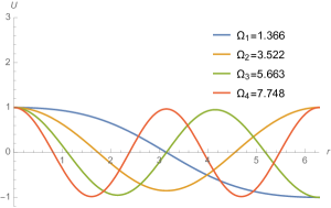
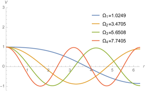
Figure 3: First four normal modes for the normal coordinates $U$ and $V$, together with the corresponding normal frequencies. Neumann boundary conditions have been imposed on the electromagnetic perturbation.

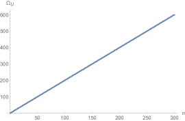
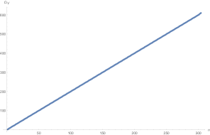
Figure 4: The spectrum of the electromagnetic perturbation. One sees that rapidly, as a function of the mode number, the frequencies tend to an equispaced, i.e. linear spectrum. The equation for the normal variable $U$ depends on the details of the background configuration. We have selected the nodeless configuration for $b_{3}^{\prime}(r)$ as a background.

The Eq. (60) can be brought into the standard Mathieu form

$$U^{\prime\prime}+(A-2Q\cos(2x))U=0\ ,$$ (64)

when the parameters are related as

$$A=\left(4K+\Omega_{U}^{2}\right)l_{1}^{2}\ ,\quad 2Q=4Kl_{1}^{2}\ .$$ (65)

The comparison with Eqs. (7) and (8) of [47] shows the correspondence between the Skyrme and Mathieu parameters:

$$\frac{2}{\hbar^{2}} = Kl_{1}^{2}\ ,\quad\left(4K+\Omega_{U}^{2}\right)l_{1}^{2}=\frac{8u}{\hbar^{2}}\ \Rightarrow$$ (66)

$$\Omega_{U}^{2} = \frac{8u}{l_{1}^{2}\hbar^{2}}-4K\ ,\quad\hbar_{eff}^{2}=\frac{2}{Kl_{1}^{2}}=\frac{32}{K\lambda}\ ,$$ (67)

where the combination $32/K\lambda$ plays the role of the “effective Planck constant” $\hbar_{eff}^{2}$ of the problem so that the parameter $u$ does not depend separately on $K$ and $\lambda$ but only on their product (as well as on the label $n$ of the discrete energy level). Well known results in the theory of the Mathieu equation can be used to determine the spectrum (in particular, the parameter $\Omega_{U}$) of the above perturbations in Eqs. (57). Let us focus on Eqs. (60), (65), (66) and (67). The results of [47] which can be applied directly to our case are (with the obvious replacement $\hbar\rightarrow\hbar_{eff}$):

1) To expand $u\left(K,\lambda;n\right)$ (or equivalently $\Omega\left(K,\lambda;n\right)^{2}$ through Eq. (67)) in power series of the effective Planck constant $\hbar_{eff}^{2}$ is not enough to get a mathematically well-defined answer. The perturbative series is not even Borel summable. However, the inclusion of non-perturbative contributions discloses the resurgent phenomenon.

2) One needs to express $u$ as a trans-series:

$$\left(u_{trans}\left(\hbar_{eff};n\right)\right)^{2}=\sum_{k=0}^{\infty}\sum_{j=0}^{\infty}\sum_{l=1}^{k-1}c_{k,j,l}\left(n\right)\left(\hbar_{eff}\right)^{j}\left(\frac{\exp\left[-\frac{S}{\hbar_{eff}}\right]}{\left(\hbar_{eff}\right)^{n+1/2}}\right)^{k}\left(\ln\left(-\frac{1}{\hbar_{eff}}\right)\right)^{l}\ ,$$ (68)

where, with the normalizations in Eqs. (7), (8) and (9) of [47] the $S$ in the exponential factors (the “instanton” action) in the above trans-series is

$$S=8\ .$$

3) The above trans-series in Eq. (68) allows to define clearly a strong coupling ($n\hbar_{eff}\gg 1$) regime and weak coupling regime ($n\hbar_{eff}\ll 1$). The corresponding expansions (reviewed in [47]) can be applied directly to the present case. We will not report these expansions here since the main aim of the present subsection is to show the explicit relations of the present gauged Skyrmion and its electromagnetic perturbations with (well-known results on) the Mathieu equation.

The analogy with the Mathieu equation analyzed in [47] is not complete since, in that reference, the Mathieu equation was interpreted as a Schrodinger equation so that the unknown function in Eq. (7) of [47] is a complex wave function satisfying the boundary conditions in Eq. (36) of the same reference. In the present case, the unknown function $U$ in Eq. (60) is real and satisfies Eq. (62). On the other hand, some of the results in [47] can be applied directly: in particular, the results which do not depend on the boundary conditions in Eq. (36) of [47] (such as the ones on the asymptotic expansions of $u\left(K,\lambda;n\right)$) hold in the present case as well. It is a quite remarkable feature of the present gauged solitons in (3+1) dimensions that the resurgent structures are so transparent in this setting. The gauged Skyrme model in (3+1) dimensions is definitely not a toy model and yet the importance of the resurgence interplay between the perturbative expansion and the non-perturbative contributions is manifest. We hope to come back on the appearance of resurgence in the gauged Skyrme model in a future publication.
On the other hand, the normal coordinate $V(r)$ is determined by equation (65) which being a Whittaker-Hill equation admits a mapping with the parameters in Eq. (50) to Eq. (54) by setting

$$\alpha^{2}=-\frac{Kq^{2}\lambda l_{1}^{2}}{8l_{2}^{2}}\ ,\qquad s=\frac{iKl_{1}l_{2}}{q}\sqrt{\frac{8}{K\lambda}}\ ,$$

$$\lambda_{0}=\frac{l_{1}^{2}}{4l_{2}^{2}}\left(16Kl_{2}^{2}+Kq^{2}\lambda+4l_{2}^{2}\Omega^{2}\right)\ ,$$

and

$$a=\frac{l_{1}^{2}}{4l_{2}^{2}}\left(16Kl_{2}^{2}+Kq^{2}\lambda+4l_{2}^{2}\Omega^{2}\right)\ ,\quad b=2Kl_{1}^{2}\ ,\quad c=\frac{Kq^{2}\lambda l_{1}^{2}}{8l_{2}^{2}}\ .$$

Consequently, the resurgence parameter in this case is

$$g^{2}=\frac{i}{2\sqrt{4c+b}}=\frac{il_{2}}{\sqrt{2K\lambda(\lambda q^{2}+4l_{2}^{2})}l_{1}}\ .$$

4.2 Heun equation and gauged time-crystals

The Skyrme configuration for time crystals reads

$$\alpha=\frac{\phi}{2}\ ,\quad\beta=H(r)\ ,\quad\rho=\frac{\omega\gamma}{2}\ ,$$

with the coordinates ordering as

$$x^{\mu}=\left(\gamma,r,t,\phi\right)\ .$$

Also in this case, a direct computation shows that, using the line element in Eq. (35), the three coupled gauged Skyrme equations (namely, $\mathit{E}^{j}=0$, $j=1$, $2$, $3$) in Eq. (5)

$$D^{\mu}\left(R_{\mu}+\frac{\lambda}{4}\left[R^{\nu},G_{\mu\nu}\right]\right)=\mathit{E}^{j}t_{j}=0$$

and the corresponding four Maxwell equations in Eq. (6) are greatly simplified by the Skyrme ansatz in Eqs. (15), (26), (25) and the gauge potential in Eq. (17).

Indeed, Eq. (5) reduce to only one Skyrme field equation (since the third Skyrme equation is identically satisfied while the first and the second are proportional):

$$\mathit{E}^{3} = 0\ ,$$

$$\mathit{E}^{1} = I_{1}P_{TC}\left[H\right]\ ,\ \mathit{E}^{2}=I_{2}P_{TC}\left[H\right]\ ,\ \ I_{1}\neq 0\ ,\ I_{2}\neq 0\ ,$$

where $I_{j}$ are real and non-vanishing while the only non-trivial Skyrme field equation $P_{TC}\left[H\right]=0$ reads

$$\begin{split}&4\left(l_{3}^{2}\left(4-\lambda\omega^{2}\right)+\frac{l_{3}^{2}}{l_{1}^{2}}X_{2}\sin^{2}(H)+\lambda\right)H^{\prime\prime}+\frac{2l_{3}^{2}}{l_{1}^{2}}X_{2}\sin(2H)H^{\prime 2}+\frac{4l_{3}^{2}}{l_{1}^{2}}\sin^{2}(H)X_{2}^{\prime}H^{\prime}\\ &+\left[\frac{1}{4}(l_{3}^{2}\omega^{2}-1)X_{2}+\frac{\lambda l_{1}^{2}}{l_{3}^{2}}(2l_{3}^{2}\omega b_{1}-2b_{3}-1)(2l_{3}^{2}\omega b_{1}-2b_{3}-l_{3}^{2}\omega^{2})\right]\sin(4H)-\frac{2l_{3}^{2}}{\lambda}X_{2}\sin(2H)=0\ ,\end{split}$$ (69)

where

$$X_{2}(r)=8\lambda\Big{(}l_{1}^{2}b_{1}(\omega-2b_{1})+\frac{2l_{1}^{2}}{l_{2}^{2}}b_{2}^{2}+\frac{l_{1}^{2}}{l_{3}^{2}}b_{3}\left(1+2b_{3}\right)\Big{)}\ .$$ (70)

The Maxwell equations are written in the same form as the previous section, where the matrix for this case is given by

$$M_{11}=2\sin^{2}(H(r))\left(4\lambda H^{\prime 2}+\frac{\lambda l_{1}^{2}}{l_{3}^{2}}\cos^{2}(H)+4l_{1}^{2}\right)\ ,$$

$$M_{13}=-\frac{\lambda\omega l_{1}^{2}}{2l_{3}^{2}}\sin^{2}(2H)\ ,$$

$$M_{22}=M_{11}+l_{3}^{2}\omega M_{13}\ ,$$

$$M_{33}=M_{11}+\frac{l_{3}^{2}\omega^{2}+1}{\omega}M_{13}\ ,$$

$$M_{31}=-l_{3}^{2}M_{13}\ ,$$

while

$$N=\left(\frac{1}{4}(M_{13}-\omega M_{11}),0,\frac{1}{4}\left(\frac{\left(2l_{3}^{2}\omega^{2}+1\right)}{\omega}M_{13}+M_{11}\right)\right).$$

When we impose the relations

$$X_{2}=\frac{\lambda l_{1}^{2}}{l_{3}^{2}}\left(l_{3}^{2}\omega^{2}-1\right)=\text{constant}\ ,\qquad b_{3}(r)=l_{3}^{2}\omega b_{1}(r)-\frac{l_{3}^{2}\omega^{2}}{4}-\frac{1}{4}\ ,$$ (71)

the field equations are reduced to

$$2\big{(}\lambda(l_{3}^{2}\omega^{2}-1)\cos^{2}(H)-4l_{3}^{2}\big{)}H^{\prime\prime}+\left(l_{3}^{2}\omega^{2}-1\right)\sin(2H)\left(l_{1}^{2}-\lambda H^{\prime 2}\right)=0\ ,$$ (72)

$$b_{1}^{\prime\prime}+\frac{K}{8}(\omega-4b_{1})\sin^{2}(H)\Big{(}l_{1}^{2}\left(\lambda\omega^{2}-8\right)-\frac{l_{1}^{2}}{l_{3}^{2}}\lambda+\frac{\lambda l_{1}^{2}}{l_{3}^{2}}(\omega^{2}l_{3}^{2}-1)\cos(2H)-8\lambda H^{\prime 2}\Big{)}=0\ .$$ (73)

Eq. (72) has the solution

$$H(r)=\frac{l_{1}}{\sqrt{\lambda}}r+h_{0}\ ,$$

with which the equation (73) becomes

$$b_{1}^{\prime\prime}+\frac{K}{8}(\omega-4b_{1})\sin^{2}(H)\Big{(}l_{1}^{2}\left(\lambda\omega^{2}-16\right)-\frac{l_{1}^{2}}{l_{3}^{2}}\lambda+\frac{\lambda l_{1}^{2}}{l_{3}^{2}}(\omega^{2}l_{3}^{2}-1)\cos(2H)\Big{)}=0\ .$$ (74)

In terms of the same variables of Eq. (42), Eq. (73) can be written as a form of confluent Heun’s equation as in the previous section. That is,

$$\frac{d^{2}y}{dx^{2}}+\Big{(}8K\lambda\ \sin^{2}x-\Delta^{2}\sin^{2}2x\Big{)}y=0\ ,$$ (75)

with a non-negative constant $\Delta\geq 0$,

$$\Delta^{2}:=\frac{K\lambda^{2}}{4}\Big{(}\omega^{2}-\frac{1}{l_{3}^{2}}\Big{)}\ .$$

In this section, we assume that $\omega^{2}\geq 1/l_{3}^{2}$. The equation (75) can be cast into the confluent Heun’s equation

$$\frac{d^{2}}{dz^{2}}Y(z)+\Big{(}\frac{\gamma}{z}+\frac{\delta}{z-1}+\epsilon\Big{)}\frac{d}{dz}Y(z)+\frac{\alpha z-q}{z(z-1)}Y(z)=0\ ,$$ (76)

where

$$z=\cos^{2}x\ ,\qquad Y(z)=e^{-\Delta z}\ y(\arccos\sqrt{z})\ ,$$

$$\gamma=\delta=1/2\ ,\qquad\epsilon=2\Delta\ ,\qquad\alpha=\Delta+2K\lambda\ ,\qquad q=\Delta/2+2K\lambda\ .$$ (77)

A general solution to this equation is known as

$$Y(z)=C_{1}\ \text{HeunC}(\Delta+2K\lambda,1/2,1/2,2\Delta,\Delta/2+2K\lambda;z)$$

$$\hskip 36.135pt+C_{2}\sqrt{z}\ \text{HeunC}(2\Delta+2K\lambda,3/2,1/2,2\Delta,3\Delta/2+2K\lambda-1/4;z)\ .$$ (78)

The confluent Heun’s function can be expanded in terms of Kummer’s confluent functions when $\epsilon\neq 0$, and $\gamma+\delta$ is not zero nor negative integer [62]. Our equation satisfies this condition so that

$$Y(z)=\sum\limits_{n=1}^{\infty}a_{n}\ {}_{1}F_{1}(n+\frac{1}{2};\ \frac{1}{2};\ -2\Delta z)\ ,$$ (79)

where ${}_{1}F_{1}$ is the Kummer’s confluent hypergeometric function, and the coefficients are determined by the recursion relation

$$n\Big{(}n-\frac{K\lambda}{\Delta}\Big{)}a_{n}+\Big{\{}-2n^{2}+\Big{(}\frac{2K\lambda}{\Delta}+2\Delta+3\Big{)}n-\Big{(}\frac{3K\lambda}{2\Delta}+2K\lambda+\frac{3\Delta}{2}+\frac{5}{4}\Big{)}\Big{\}}a_{n-1}$$

$$+\Big{(}n-\frac{3}{2}\Big{)}\Big{(}n-\frac{3}{2}-\frac{K\lambda}{\Delta}\Big{)}a_{n-2}=0\ .$$ (80)

It is worth to notice that this kind of series is terminated if

$$\frac{K\lambda}{\Delta}=N+\frac{1}{2}\ ,$$ (81)

$$\Rightarrow \ \omega(N)=\pm\Big{(}\frac{1}{l_{3}^{2}}+\frac{4K}{(N+1/2)^{2}}\Big{)}^{1/2}\ ,$$ (82)

for some natural number $N\in\mathbb{N}$.

A possible criticism to the time-crystals constructed in the previous references [35], [36] is that there was no argument to fix the corresponding time-periods. It is a very intriguing results that the classic theory of Kummer’s confluent functions is able to fix the time-period of the present gauged time-crystals based on the Heun equation through the quantization condition in Eq. (82).

4.2.1 Relation with the Whittaker-Hill equation

Following the same steps as the gauged Skyrmion, the mapping with the Whittaker-Hill equation

$$y^{\prime\prime}+\left(\lambda_{0}+4\alpha s\cos{(2x)}+2\alpha^{2}\cos{(4x)}\right)y=0\ ,$$

determines the coefficients as

$$\lambda_{0}=\frac{K\lambda}{8l_{3}^{2}}\left(\lambda-l_{3}^{2}(\lambda\omega^{2}-32)\right)\ ,\quad\alpha^{2}=\frac{K\lambda^{2}}{16l_{3}^{2}}\left(l_{3}^{2}\omega^{2}-1\right)\ ,\quad s=-4l_{3}\sqrt{\frac{K}{l_{3}^{2}\omega^{2}-1}}\ ,$$

so that, the resurgence parameter is given by

$$g^{2}=l_{3}\left(\lambda K(l_{3}^{2}\lambda\omega^{2}-8l_{3}^{2}-\lambda)\right)^{-1/2}\ .$$

5 Conclusions and perspectives

We have shown that one can get a complete analytic description of gauged Skyrmions in (3+1) dimensions living within a finite volume in terms of classic results in the theory of ordinary differential equations. In particular, we have been able to reduce the coupled field equations of the gauged Skyrme model (which, in principle, are seven coupled non-linear PDEs) in two non-trivial topological sectors (one corresponding to gauged Skyrmions and the other to gauged time-crystals) to the Heun equation (which, for some particular choice of the parameters, can be further reduced to the Whittaker-Hill equation). This technical result has many intriguing consequences. First of all, one obtains a complete explicit construction of these gauged solitons in terms of Heun and Kummer functions (so that, for instance, it is possible to compute the energy of the system in terms of the Baryon charge and the volume of the region). Secondly, the time-period of the time-cystals is quantized. Likewise, the volume occupied by the gauged Skyrmions is quantized. The present analysis also discloses the appearance of resurgent phenomena within the gauged Skyrme model in (3+1) dimensions. In particular, suitable electromagnetic perturbations of the gauged Skyrmions satisfy the Mathieu equation (which is a well known example in which the resurgent paradigm works very well). Thus, the spectrum of these perturbations can be determined in terms of known results in the theory of the Mathieu equation.

It is worth to further analyze the appearance of resurgent phenomena in the Skyrme model as this analysis could help to shed new light on resurgence in QCD as well. We hope to come back on this important issue in a future publication.

Acknowledgements

M.L. and A.V. appreciates the support of CONICYT Fellowship 21141229 and 21151067, respectively. This work has been funded by the FONDECYT grants 1160137 and 1181047. The Centro de Estudios Científicos (CECs) is funded by the Chilean Government through the Centers of Excellence Base Financing Program of CONICYT. The work is supported in part by National Research Foundation of Korea funded by the Ministry of Education (Grant 2018-R1D1A1B0-7048945).

References

- [1] E. Witten, Nucl. Phys. B 223 (1983), 422; Nucl. Phys. B 223 (1983), 433.
- [2] T. Skyrme, Proc. R. Soc. London A 260, 127 (1961); Proc. R. Soc. London A 262, 237 (1961); Nucl. Phys. 31, 556 (1962).
- [3] D. Finkelstein, J. Rubinstein, J. Math. Phys. 9, 1762–1779 (1968).
- [4] N. Manton and P. Sutcliffe, Topological Solitons, (Cambridge University Press, Cambridge, 2007).
- [5] H. Weigel, Chiral Soliton Models for Baryons, Lecture Notes in Physics (Springer, 2008)
- [6] V. G. Makhanov, Y. P. Rybakov, V. I. Sanyuk, The Skyrme model, Springer-Verlag (1993).
- [7] D. Giulini, Mod. Phys.Lett. A8, 1917–1924 (1993).
- [8] A.P. Balachandran, A. Barducci, F. Lizzi, V.G.J. Rodgers, A. Stern, Phys. Rev. Lett. 52 (1984), 887.
- [9] G. S. Adkins, C. R. Nappi, E. Witten, Nucl. Phys. B 228 (1983), 552-566.
- [10] E. Guadagnini, Nucl. Phys. B 236 (1984), 35-47.
- [11] I. Klebanov, Nucl. Phys. B 262 (1985) 133.
- [12] A. Actor, Phys. Lett. B 157 (1985) 53.
- [13] H. A. Weldon, Phys. Rev. D 26 (1982) 1394.
- [14] M. Loewe, S. Mendizabal, J.C. Rojas, Phys. Lett. B 632 (2006) 512.
- [15] J. A. Ponciano, N. N. Scoccola, Phys. Lett. B 659 (2008) 551.
- [16] C. G. Callan Jr. and E. Witten, Nucl. Phys. B 239 (1984) 161-176.
- [17] J.M. Gipson and H.Ch. Tze, Nucl. Phys. B 183 (1981) 524.
- [18] J. Goldstone and F. Wilczek, Phys. Rev. Lett. 47 (1981) 986.
- [19] E. D’Hoker and E. Farhi, Nucl. Phys. B241 (1984) 109.
- [20] V.A. Rubakov, Nucl. Phys. B256 (1985) 509.
- [21] B.M.A.G. Piette, D. H. Tchrakian, Phys.Rev. D 62 (2000) 025020.
- [22] E. Radu, D. H. Tchrakian, Phys. Lett. B 632 (2006) 109–113.
- [23] F. Canfora, H. Maeda, Phys. Rev. D 87, 084049 (2013).
- [24] F. Canfora, Phys. Rev. D 88, 065028 (2013).
- [25] F. Canfora, F. Correa, J. Zanelli, Phys. Rev. D 90, 085002 (2014).
- [26] F. Canfora, A. Giacomini, S. Pavluchenko, Phys. Rev. D 90, 043516 (2014).
- [27] S. Chen, Y. Li, Y. Yang, Phys. Rev. D 89 (2014), 025007.
- [28] E. Ayon-Beato, F. Canfora, J. Zanelli, Phys. Lett. B 752, (2016) 201-205.
- [29] F. Canfora, G. Tallarita, Nucl. Phys. B 921 (2017) 394.
- [30] F. Canfora, G. Tallarita, Phys. Rev. D 94, 025037 (2016).
- [31] A. Giacomini, M. Lagos, J. Oliva and A. Vera, Phys. Lett. B 783, 193 (2018).
- [32] F. Canfora, G. Tallarita, Phys. Rev. D 91, 085033 (2015).
- [33] F. Canfora, G. Tallarita, JHEP 1409, 136 (2014).
- [34] F. Canfora, Seung Hun Oh, P. Salgado-Rebolledo, Phys. Rev. D96 (2017), 084038.
- [35] P. D. Alvarez, F. Canfora, N. Dimakis and A. Paliathanasis, Phys. Lett. B773, (2017) 401-407.
- [36] L. Aviles, F. Canfora, N. Dimakis, D. Hidalgo, Phys. Rev. D96 (2017), 125005.
- [37] I. Aniceto, G. Başar, R. Schiappa, A Primer on Resurgent Transseries and Their Asymptotics, arXiv:1802.10441.
- [38] J. C. Le Guillou and J. Zinn-Justin, Large order behavior of perturbation theory, (North-Holland, Amsterdam, 1990).
- [39] M. V. Berry and C. J. Howls, Proc. R. Soc. A 430, 653 (1990); Proc. R. Soc. A 434, 657 (1991); M. V. Berry, ”Asymptotics, Superasymptotics, Hyperasymptotics …”, in Asymptotics Beyond All Orders, H. Segur et al (Eds), (Plenum Press, New York, 1991).
- [40] M. Marino, R. Schiappa, and M. Weiss, Commun. Num. Theor. Phys. 2 (2008) 349; J. Math. Phys. 50, 052301 (2009).
- [41] E. B. Bogomolny, Phys. Lett. B 91, 431 (1980).
- [42] J. Zinn-Justin, Nucl. Phys. B 192, 125 (1981).
- [43] I. Aniceto, R. Schiappa, Comm. Math. Phys. 335, 183–245 (2015).
- [44] I. Aniceto, J. Russo, R. Schiappa, JHEP 1503 (2015) 172.
- [45] S. Demulder, D. Dorigoni and D. C. Thompson, JHEP 1607, 088 (2016).
- [46] G. Basar, G. V. Dunne, JHEP 1502, 160 (2015),
- [47] G. V. Dunne and M. Unsal, arXiv:1603.04924 [math-ph].
- [48] F. Wilczek, Phys. Rev. Lett. 109, 160401 (2012).
- [49] A. Shapere, F. Wilczek, Phys. Rev. Lett. 109, 160402 (2012).
- [50] F. Wilczek, Phys. Rev. Lett. 111, 250402 (2013).
- [51] P. Bruno, Phys. Rev. Lett. 111, 070402 (2013); Phys. Rev. Lett. 110, 118901 (2013); Phys. Rev. Lett. 111, 029301 (2013).
- [52] H. Watanabe, M. Oshikawa, Phys. Rev. Lett. 114, 251603 (2015).
- [53] K. Sacha, J. Zakrzewski, ”Time crystals: a review” arXiv: 1704.03735.
- [54] K. Sacha, Phys. Rev. A 91, 033617 (2015).
- [55] S. Choi, J. Choi, R. Landig, G. Kucsko, H. Zhou, J. Isoya, F. Jelezko, S. Onoda, H. Sumiya, V. Khemani, C. von Keyserlingk, N. Y. Yao, E. Demler, M. D. Lukin, Nature 543 (7644), 221–225 (2017), letter.
- [56] Zhang, J, P. W. Hess, A. Kyprianidis, P. Becker, A. Lee, J. Smith, G. Pagano, I.-D. Potirniche, A. C. Potter, A. Vishwanath, N. Y. Yao, C. Monroe, Nature 543 (7644), 217–220 (2017), letter.
- [57] N. Y. Yao, A. C. Potter, I.-D. Potirniche, A. Vishwanath, Phys. Rev. Lett. 118, 030401 (2017).
- [58] D. V. Else, B. Bauer, C. Nayak, Phys. Rev. Lett. 117, 090402 (2016); Phys. Rev. Lett. 118, 030401 (2017).
- [59] V. Khemani, A. Lazarides, R. Moessner, S. L. Sondhi, Phys. Rev. Lett. 116, 250401 (2016).
- [60] A. D. Hemery, A. P. Veselov, Journal of Mathematical Physics 51 (2010) 072108.
- [61] W. Magnus and S. Winkler, Hill‘s equation, Interscience tracts in pure and applied mathematics (Interscience, New York, 1966).
- [62] T. A. Ishkhanyan and A. M. Ishkhanyan, AIP Advances 4, 087132 (2014)