figure \cftpagenumbersofftable
Speckle Statistics in Adaptive Optics Images at Visible Wavelengths
Abstract
Residual speckles in adaptive optics (AO) images represent a well-known limitation to the achievement of the contrast needed for faint sources detection. Speckles in AO imagery can be the result of either residual atmospheric aberrations, not corrected by the AO, or slowly evolving aberrations induced by the optical system. In this work we take advantage of the high temporal cadence (1 ms) of the data acquired by the SHARK-VIS forerunner experiment at the Large Binocular Telescope (LBT), to characterize the AO residual speckles at visible wavelengths. An accurate knowledge of the speckle pattern and its dynamics is of paramount importance for the application of methods aimed at their mitigation. By means of both an automatic identification software and information theory, we study the main statistical properties of AO residuals and their dynamics. We therefore provide a speckle characterization that can be incorporated into numerical simulations to increase their realism, and to optimize the performances of both real-time and post-processing techniques aimed at the reduction of the speckle noise.
Address all correspondence to: M. Stangalini, INAF-OAR Via Frascati 33, 00078 Monte Porzio Catone, (RM) Italy; E-mail: \linkablemarco.stangalini@inaf.it
1 Introduction
Speckle noise represents one of the major limitations to the detection of faint companions to nearby stars [1]. Although current high contrast imaging instruments and coronagraphs make all use of sophisticated and high performance AO systems [2], small optical imperfections yield quasi-static speckles and residual stray light, that can still represent a severe limitation to the achievement of the high contrast needed to detect faint companions [3, 4, 5, 6]. For these reasons, a deep understanding of the speckle variability and statistics is of fundamental importance for the optimization of post-facto techniques aimed at increasing the image contrast [7, 8, 9], like angular differential imaging (ADI), locally optimized combination of images (LOCI), or principal component analysis (PCA) [10, 11, 12, 13]. In addition, it has been demonstrated that speckle intensity statistics represents a powerful tool for speckle discrimination and, therefore, for their post-facto suppression[14].
In order to detect a Earth-like planet at close angular distance from a bright star, a flux contrast of the order of is required. Unfortunately, a final (after post-processing) contrast larger than cannot be currently expected even in AO assisted coronagraphic systems operated under the best seeing conditions at SWIR (Short-wave infrared) wavelengths [8]. Furthermore, an accurate knowledge of the speckle pattern and its dynamics is crucial to increase the realism of simulations aimed at optimizing the instrument performance.
The analysis of the dynamical behaviour of AO residuals can be used to estimate the decorrelation time of the atmospheric turbulence and thus its predictability horizon. In Ref. 6 it was recently shown that one of the major limitations to the achievement of the very high contrast needed in exoplanet imaging is represented by the servo-lag error in the ExAO (extreme adaptive optics) systems. Indeed, even a short time lag of or ms, can result in a large decrease of the bandwidth of the system, and thus of the overall performances and contrast. In Ref. 15 and, more recently, in Ref. 16 it has been demonstrated that over timescales consistent with the frozen flow approximation, the wavefront aberrations are predictable. In particular, in Ref. 16 it was shown that of the power spectral density of wavefront fluctuations is due to frozen flow. In order to mitigate the effects of the servo-lag error, several authors have proposed AO control schemes based on different forecasting approaches. See for instance Refs. 17, 18, 19, to mention a few. Very recently, the validity of this approach has been demonstrated on-sky [20]. The study of the dynamics of AO residuals and their decorrelation time is also useful to investigate the limits of applicability of such techniques.
Several authors have already investigated the statistical properties of speckles in AO corrected images [21, 22, 23, 24].
However, as of now, these statistical studies have mostly focused on intensity fluctuations in specific locations of the focal plane, using data sequences with a limited temporal cadence ( ms), longer than the typical atmospheric timescales ( ms). Recently other authors [9] have investigated the speckle lifetime in the H-band, by exploiting a Hz cadence set of extreme AO (ExAO) images.
In order to complement these studies, in this work we exploit new data acquired by the SHARK forerunner experiment [25, 26, 27, 28] at very high cadence (1 ms), and visible wavelengths. This data allows us to study the behavior of residual AO speckles down to very short timescales, and assess the atmospheric clearance time with very high accuracy. In addition we also exploit these data to study the spatial distribution of long-lived speckles which, as already mentioned, represent a severe limitation to the achievement of very high contrast in ADI images.
2 Data set
The data set used in this work consists of a series of 1 ms exposure images of the target Gliese 777 (1 ms cadence), acquired with the SHARK forerunner experiment at LBT on June 4, 2015 (see upper panels of Fig. 2). The pixel scale is set at mas, and the imager is a Zyla CMOS camera manufactured by Andor Inc111http://www.andor.com/. The total duration of the data series is min (or equivalently 1200000 images). During the acquisition the LBTI-AO system [29] was correcting 500 modes in closed loop. The AO frequency was 1 KHz with a loop delay of ms. In this conditions the closed loop db bandwidth is Hz. The seeing was in the range arcsec, and no field de-rotator is employed on the mount to correct for the sky rotation.
The SHARK-VIS Forerunner experiment is a set of short test observations performed at the LBT telescope to verify its AO system performance at visible wavelengths ( nm) between February and June 2015 [28]. The experimental setup is minimal and composed by only two optical elements before the detector: one divergent lens to get a super sampling (twice the Nyquist limit) of the PSF (point spread function) and a nm FWHM filter centered at nm. The AO control and wavefront sensing is left to the LBTI Adaptive Optics subsystem fed through a beam splitter. All the forerunner hardware is placed on a steel optical breadboard for an easy customization, and attached to the LBT main structure. Data acquisition is performed using an in house developed LabView software interfacing the Andor Zyla sCMOS (Scientific CMOS) camera with a camera link to a PCI board yielding a maximum throughput of 140 Mpixel/s digitized at bit. The short exposure time (1 ms) is used to freeze the evolution of atmospheric speckles and to easily recover the residual jitter in the focal plane, for its post-facto correction. We remark here that residual jitter in longer exposure images may affect the results of the statistical analysis of residual speckles. Our very fast cadence allows us to reduce this effect by employing a post-facto registration of the data sequence.
Our target is acquired at low Zenith angles to avoid PSF elongation due to atmospheric differential refraction, and close to the meridian to maximize the effect of field rotation useful for ADI post processing of image stacks.
The data calibration process consists of the dark frame subtraction and image registration through a FFT (Fast Fourier Transform) phase correlation technique. In short, the FFT cross correlation between the two images is computed, and the phase is estimated from it. For two perfectly matching images, the cross-phase is a function with a peak at the center of the image domain. When one of the two images is shifted with respect to the other, the position of the peak of the phase function is shifted by an amount of pixels corresponding to the exact shift between the two images themselves. By fitting a gaussian to the phase function it is possible to estimate the shift (i.e. the position of its peak) with sub-pixel accuracy.
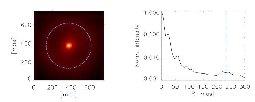
In the left panel of Fig. 1, we show an image of the target obtained by adding up to 1200000 unsaturated images after their sub-pixel registration. This is equivalent to a 20 min exposure time. In the same figure (right panel) we also show a radial profile of the same long-exposure PSF.
In this work we focus our attention on both regions within and outside the radius at which the AO system is effectively suppressing the atmospheric aberrations. This corresponds to a distance from the optical axis which is commonly referred to as control radius [30], and depends on the number of actuators of the DM (deformable mirror), the wavelength, and telescope diameter. The control radius is represented by the dashed line in Fig. 1. At larger radial distances the DM is not able to suppress aberration modes, and the PSF is dominated by seeing.
The speckles within the control radius, are those which are due to either AO residual aberrations, and quasi-static distortions due, for example, to NCPA (non common path aberrations). Hereafter we refer to these speckles as AO residuals, while we refer to the speckles outside the control radius as seeing-induced speckles. However, it is worth mentioning here that the SHARK forerunner is designed to minimize NCPA aberrations by simplifying its optical path and picking the beam off very close to the WFS [25, 27].

Further, during the observation, the NCPAs aberrations where mitigated by injecting an offset on the secondary deformable mirror of LBT following the procedure described in Ref. 31.
3 Methods and Results
3.1 Speckle lifetime statistics
In order to estimate the lifetime of the two populations of speckles within and outside the control radius (i.e. AO residuals and seeing-induced respectively), speckles are identified and tracked by using the SWAMIS tracking code [32]. This code was originally written for the identification and tracking of small scale magnetic elements in the solar photosphere [33, 34, 35]; a task conceptually similar to that of the analysis of AO residual faint speckles in SHARK forerunner data [36, 37]. In short, the code identifies and tracks, through sequential images, small scale features which are above a user specified threshold ( in our case), where is the standard deviation of the signal (intensity) computed in a dark region in the upper left corner of the image, and covering at least an area of n pixels (where in our case). This implies that only structures with a size of the order of the PSF are identified and tracked, thus ruling out the possibility to include noise features. In order for a speckle to be uniquely identified, this two thresholds have to be met at the same time.
With the aim of reducing the computational time, instead of using the entire set of images (1200000), we limit ourselves to the analysis of different temporal windows of 5 s (5000 images) during the observation run.
Indeed, even if looking at this short interval, the number of speckles identified and matching the above criteria amounts to about . This is a large number ensuring a good estimation of the underlying statistics.
Here we focus our attention to the first temporal window at the beginning of the data sequence, while at the end of this section we will extend the analysis to the other temporal windows.
After the identification of the speckles matching the searching criteria, the code assigns a label to each of them. This label is unique throughout the data series and permits the identification of the speckles at different time steps. In the lower panels of Fig. 2, we show an example of masks obtained from the identification of the speckles in the images shown in the upper panels of the same figure. In the same panels, we also show the labels of each speckle, which represents its unique identifier during its entire life.
In order to distinguish possible differences between the two populations of speckles, we separate them into two classes: those lying within the control radius, and those outside (see blue dashed line in Fig. 1), and measure, for each of them, the lifetime and the maximum intensity throughout their entire life.
It is worth noting that the selection criteria described above do not allow the code to single out speckles in proximity of the center of the PSF (see lower panels of Fig. 2). Despite this, a large amount of speckles are identified within the control radius anyway, thus ensuring the statistical significance of the results.
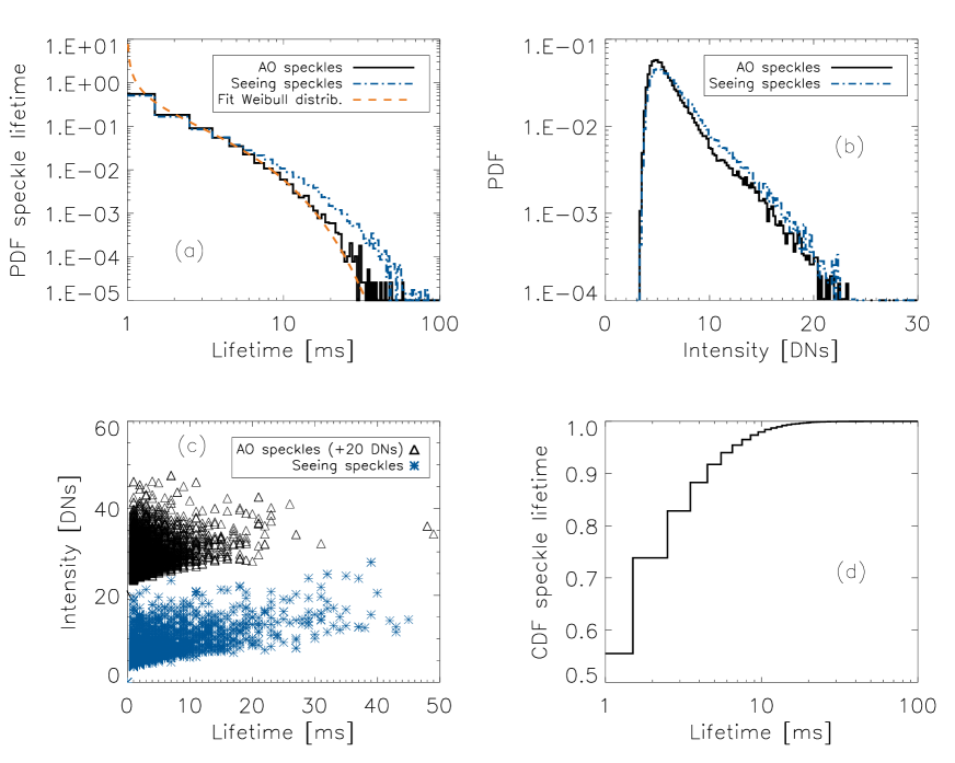
In panel (a) of Fig. 3 we show the probability density function (PDF) of lifetimes for the two samples of speckles. As one can note from the same figure, the PDF can be modeled by a 2-parameter Weibull distribution [38] of the form:
| (1) |
where is the time, a shape parameter, and a scaling parameter, also known as characteristic time. The least squares fit to the data yields and ms. It is worth recalling that, by definition, the time scale of the Weibull distribution represents the time at which of the sampled population die.
Apart from the physical meaning (Weibull distributions are usually found in turbulence as the signature of random multiplicative processes [39]), this represents a simple form that can be easily incorporated into numerical simulations of high contrast coronagraphic imagers, to improve the accuracy of their estimated contrast.
It is worth noting that the PDF of the lifetimes of seeing-induced speckles, as compared to that of the AO residuals, shows a larger density of elements in the range ms, if compared to the PDF of the AO residuals. This is in agreement with previous results in literature showing that the AO system only modifies the intensity of speckles, leaving their lifetime unchanged[4]. Indeed, this effect can be due to the intensity threshold used for the identification of the speckles. In panel (b) of the same figure we show that the PDF of the intensity of the seeing-induced speckles presents an intrinsically larger amount of elements, with respect to the intensity distribution of AO residuals, in the bright end. In the presence of an almost linear dependence of the lifetime on the intensity (see panel c of the same figure), this translates into an increase of the probability of detection of long-lived speckles outside the control radius of the PSF. Brighter speckles remain above the selection threshold longer than the fainter ones, resulting in an increase of the fraction of the identified longest-lived speckles themselves. However, except for this increase, the two PDFs do not show significant differences.
Another important aspect by far is the estimation of the atmospheric refreshing time, that is the time over which the speckle pattern is completely renewed.
To this regard, in panel (b) of Fig. 3 we show the CDF (cumulative distribution function) of the AO speckle lifetime. The CDF represents the probability of finding a speckle with a lifetime shorter than . The CDF shows that while of the speckles identified have a lifetime of the order of ms, of them are found within ms. This means that after this time, the speckle pattern is almost completely renewed, and this value can be considered as the refreshing time scale of the atmospheric turbulence.
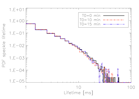
The above results were obtained by analyzing a temporal window of s at the beginning of the data sequence ( min). In order to be sure that the statistics does not depend on the particular temporal window selected, as already mentioned we repeated the analysis over different temporal windows (i.e. , min, and min). The results of this analysis are shown if Fig. 4 where we plot the PDFs of the speckle lifetime for each temporal window selected. This plot shows that the PDF of lifetimes does not change significantly during the observation.
3.2 Mutual information and memory of the process
In order to independently check the above results, we make use of a completely different approach based upon information theory [40]. More in particular, we make use of the mutual information (MI) [41, 42], which is a measure of the non-linear mutual dependence of two variables and , and defined as:
| (2) |
where represents the joint probability function, and and the probability density functions of and , respectively. It is a well known result that, while the correlation is a measure of the linear dependence between two variables, mutual information is a more general quantity that can be applied also to non-linear processes [43]. MI was already employed in the adaptive optics field, in the optimization of the wavefront reconstruction [44].
Since the statistics of speckles does not change during the observation, here we focus on the first temporal window analysed at the beginning of the previous section.
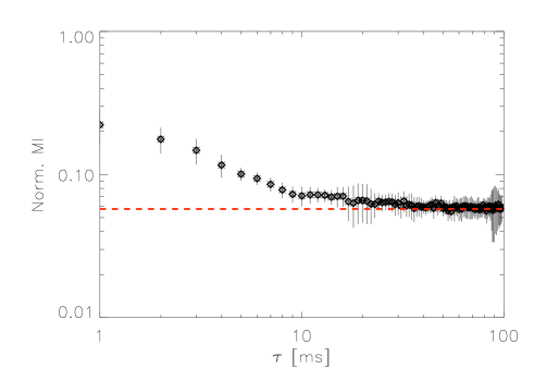
We divided the first s of the observations into short subsequences of ms each. This is possible since in ms the speckle pattern is completely refreshed. For each subsequence, we estimated the MI between the first and any other following image. This is done by only considering the region of the FoV within the control radius which is marked by the dashed blue line of Fig. 1. In Fig. 5 we plot the average MI as a function of the delay . We stress here that this analysis is only made possible by the high cadence of the data. As expected, MI undergoes a rapid decrease as the time delay goes by. This indicates a rapid decrease of correlation of the process with time. After ms, MI reaches an asymptotic value, indicating the presence of a persistent pattern of residues. Most of the speckles have a very short lifetime (shorter than ms) and, consequently, the MI drops by almost in ms ( for by definition). The rapid reduction of MI reflects the short memory of the process associated with the evolution of the atmospheric turbulence, which determines a fast evolution of the speckle pattern. Indeed, after ms the speckle pattern is completely renewed, and the mutual dependence between the current and the first PSFs is reduced at minimum. However, it is worth noting that the asymptotic value of the MI is not zero, as expected for statistically independent images. As already anticipated, this implies that there exists a quasi-static component of the pattern itself. However, this component accounts for only of the total information contained in the speckle images. We note that the estimated value of the decorrelation time obtained through MI, is in good agreement with that estimated by the PDF of the lifetimes seen in the previous section.
It is interesting to note that the error bars in the plot, representing the standard errors of the mean of the sequences, oscillate in size reflecting the intrinsic spread of the MI estimated from the different sequences.
3.3 Spatial distribution of quasi-static speckles
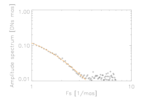
In order to further investigate the nature of AO residual speckles, we also analyse their spatial distribution by estimating the FFT spatial spectra of intensity fluctuations. More in particular, we focus our attention on the spatial distribution of the longest-lived components of the intensity fluctuations with the aim of investigating the character of quasi-static speckles. If images are averaged over a sufficiently longer time (say times the clearance time), we expect to significantly reduce the contribution from seeing-induced and rapidly disappearing speckles, with only the ones commonly referred to as quasi-static speckles left in the images. In order to study the spatial contribution of this latter component, we average our entire data sequence (20 min duration) in windows of ms to get rid of the rapidly evolving speckle component. For each of this ”long exposure” images, we estimate the spatial FFT spectrum, after masking out pixels outside the control radius, over which the DM has no effect. The masking is performed with a gently decreasing function without sharp edges to avoid side effects in the FFTs (, where represents the Hanning window centered at the PSF peak). We then consider the average amplitude spectrum of the spatial fluctuations as our best estimate of the quasi-static speckles spatial distribution in the Fourier space. The spatial spectrum of the fluctuations due to quasi-static speckles can be modeled as follows [45]:
| (3) |
where represents the spatial frequency.
In Fig. 6 we show the mean amplitude of the spatial spectrum of residual speckles. A least squares fit of the above model to the data in the range mas-1 yields the following estimates for the three parameters: , , and .
4 Concluding remarks
Our results show that the turbulence clearance time at visible wavelength is of the order of ms. Indeed, of the statistical sample of speckles detected in our data have a lifetime shorter than this value. The CDF of the speckles lifetime shows that those with a lifetime longer than ms are very few; only speckle/s. In addition, the PDF of the lifetime of the AO residual speckles is found to be well represented by a Weibull distribution. This is not surprising since this distribution is generally used to model lifetimes of different physical processes in a wide range of contexts [38]. However, it is worth stressing here that the accurate modeling of the PDF of lifetimes is only made possible by the high frame rate of the SHARK-VIS forerunner experiment that, delivering images with a cadence of 1 ms, freezes the atmospheric turbulence evolution. The clearance time of the atmospheric turbulence is estimated in this work through two different approaches (automatic speckle identification and information theory) from closed-loop AO images and can be regarded as a decorrelation time scale of the spatial pattern of speckles. After this time, the speckle pattern is completely regenerated.
Our results demonstrate that at least in these particular observing conditions, the decorrelation time of the atmospheric aberrations is much longer than the AO correction frequency (1 kHz). It is worth noting here that of the speckles have a lifetime shorter than 5 ms, thus the overall predictability horizon of the wavefront aberrations must lie in this range. In other words, at visible wavelengths, most of the memory of the system is already lost after 5 ms, thus this sets an intrinsic limit to the predictability of the process which is much shorter than the decorrelation time. This is important for the implementation of AO predictive control schemes in the visible.
In addition to this, we also estimated the spatial distribution of the quasi-static speckles, after averaging out the seeing-induced ones. The power spectrum of the quasi-static speckles is well represented by the model proposed in Ref. 45. However, in this work we are able to provide an accurate estimate of their parameters thanks to the high cadence of our data.
This piece of information is important to increase the realism of end-to-end AO simulations for the assessment of the performances of high contrast imagers in real on-sky conditions.
It is worth noting that our characterization of the speckle statistics is based on a particular set of observing conditions. However, we also note that this is the first time that seeing induced residual speckles are characterized down to time scales as small as 1 ms. This is due to the high acquisition cadence of the SHARK forerunner that allowed us to perform a detailed characterization of the dynamics of the speckles themselves.
Acknowledgements.
The LBT is an international collaboration among institutions in the United States, Italy and Germany. LBT Corporation partners are: Istituto Nazionale di Astrofisica, Italy; The University of Arizona on behalf of the Arizona Board of Regents; LBT Beteiligungsgesellschaft, Germany, representing the Max-Planck Society, The Leibniz Institute for Astrophysics Potsdam, and Heidelberg University; The Ohio State University, and The Research Corporation, on behalf of The University of Notre Dame, University of Minnesota and University of Virginia. This work was partially funded by ADONI, the ADaptive Optics National laboratory of Italy, and by the European Commission’s H2020 project GREST, grant agreement n. 653982.References
- [1] R. Racine, G. A. H. Walker, D. Nadeau, R. Doyon, and C. Marois, “Speckle Noise and the Detection of Faint Companions,” PASP 111, 587–594 (1999).
- [2] E. Hugot, M. Ferrari, K. El Hadi, A. Costille, K. Dohlen, P. Rabou, P. Puget, and J. Beuzit, “Active optics methods for exoplanet direct imaging-stress polishing of supersmooth aspherics for vlt-sphere planet finder,” Astronomy & Astrophysics 538, A139 (2012).
- [3] C. Marois, R. Doyon, R. Racine, and D. Nadeau, “Efficient speckle noise attenuation in faint companion imaging,” Publications of the Astronomical Society of the Pacific 112(767), 91–96 (2000).
- [4] B. Macintosh, L. Poyneer, A. Sivaramakrishnan, and C. Marois, “Speckle lifetimes in high-contrast adaptive optics,” in Optics & Photonics 2005, 59030J–59030J, International Society for Optics and Photonics (2005).
- [5] C. Cavarroc, A. Boccaletti, P. Baudoz, T. Fusco, and D. Rouan, “Fundamental limitations on earth-like planet detection with extremely large telescopes,” Astronomy & Astrophysics 447(1), 397–403 (2006).
- [6] M. Kasper, “Adaptive optics for high contrast imaging,” in Society of Photo-Optical Instrumentation Engineers (SPIE) Conference Series, Society of Photo-Optical Instrumentation Engineers (SPIE) Conference Series 8447, 0 (2012).
- [7] P. Martinez, C. Loose, E. Aller Carpentier, and M. Kasper, “Speckle temporal stability in XAO coronagraphic images,” A&A 541, A136 (2012).
- [8] P. Martinez, M. Kasper, A. Costille, J. F. Sauvage, K. Dohlen, P. Puget, and J. L. Beuzit, “Speckle temporal stability in XAO coronagraphic images. II. Refine model for quasi-static speckle temporal evolution for VLT/SPHERE,” A&A 554, A41 (2013).
- [9] J. Milli, T. Banas, D. Mouillet, D. Mawet, J. Girard, A. Vigan, A. Boccaletti, M. Kasper, Z. Wahhaj, A. Lagrange, et al., “Speckle lifetime in xao coronagraphic images: temporal evolution of sphere coronagraphic images,” in SPIE Astronomical Telescopes+ Instrumentation, 99094Z–99094Z, International Society for Optics and Photonics (2016).
- [10] C. Marois, D. Lafrenière, R. Doyon, B. Macintosh, and D. Nadeau, “Angular Differential Imaging: A Powerful High-Contrast Imaging Technique,” ApJ 641, 556–564 (2006).
- [11] D. Lafrenière, C. Marois, R. Doyon, D. Nadeau, and É. Artigau, “A New Algorithm for Point-Spread Function Subtraction in High-Contrast Imaging: A Demonstration with Angular Differential Imaging,” ApJ 660, 770–780 (2007).
- [12] R. Soummer, L. Pueyo, and J. Larkin, “Detection and Characterization of Exoplanets and Disks Using Projections on Karhunen-Loève Eigenimages,” ApJ 755, L28 (2012).
- [13] A. Amara and S. P. Quanz, “PYNPOINT: an image processing package for finding exoplanets,” MNRAS 427, 948–955 (2012).
- [14] S. Gladysz, N. Yaitskova, and J. C. Christou, “Statistics of intensity in adaptive-optics images and their usefulness for detection and photometry of exoplanets,” Journal of the Optical Society of America A 27, A64–A75 (2010).
- [15] M. B. Jorgenson and G. J. M. Aitken, “Prediction of atmospherically induced wave-front degradations,” Optics Letters 17, 466–468 (1992).
- [16] L. Poyneer, M. van Dam, and J.-P. Véran, “Experimental verification of the frozen flow atmospheric turbulence assumption with use of astronomical adaptive optics telemetry,” Journal of the Optical Society of America A 26, 833 (2009).
- [17] N. J. Doelman, K. J. G. Hinnen, F. J. G. Stoffelen, and M. H. Verhaegen, “Optimal control strategy to reduce the temporal wavefront error in AO systems,” in Advancements in Adaptive Optics, D. Bonaccini Calia, B. L. Ellerbroek, and R. Ragazzoni, Eds., Society of Photo-Optical Instrumentation Engineers (SPIE) Conference Series 5490, 1426–1437 (2004).
- [18] M. Stangalini, F. Berrilli, D. Del Moro, and R. Piazzesi, “Multiple field-of-view MCAO for a Large Solar Telescope: LOST simulations,” in Society of Photo-Optical Instrumentation Engineers (SPIE) Conference Series, Society of Photo-Optical Instrumentation Engineers (SPIE) Conference Series 7736, 4 (2010).
- [19] K. Jackson, C. Correia, O. Lardière, D. Andersen, and C. Bradley, “Linear prediction of atmospheric wave-fronts for tomographic adaptive optics systems: modelling and robustness assessment,” Optics Letters 40, 143 (2015).
- [20] J. Tesch, T. Truong, R. Burruss, and S. Gibson, “On-sky demonstration of optimal control for adaptive optics at palomar observatory,” Optics letters 40(7), 1575–1578 (2015).
- [21] C. Aime and R. Soummer, “The Usefulness and Limits of Coronagraphy in the Presence of Pinned Speckles,” ApJ 612, L85–L88 (2004).
- [22] C. Aime and R. Soummer, “The effect of a coronagraph on the statistics of Adaptive Optics Pinned Speckles,” in EAS Publications Series, C. Aime and R. Soummer, Eds., EAS Publications Series 12, 89–101 (2004).
- [23] M. P. Fitzgerald and J. R. Graham, “Speckle Statistics in Adaptively Corrected Images,” ApJ 637, 541–547 (2006).
- [24] N. Yaitskova and S. Gladysz, “First-order speckle statistics for arbitrary aberration strength,” Journal of the Optical Society of America A 28, 1909–1919 (2011).
- [25] M. Stangalini, F. Pedichini, M. Centrone, S. Esposito, J. Farinato, E. Giallongo, F. Quirós-Pacheco, and E. Pinna, “The solar system at 10 parsec: exploiting the ExAO of LBT in the visual wavelengths,” in Society of Photo-Optical Instrumentation Engineers (SPIE) Conference Series, Society of Photo-Optical Instrumentation Engineers (SPIE) Conference Series 9147, 8 (2014).
- [26] J. Farinato, F. Pedichini, E. Pinna, F. Baciotti, C. Baffa, A. Baruffolo, M. Bergomi, P. Bruno, E. Cappellaro, L. Carbonaro, A. Carlotti, M. Centrone, L. Close, J. Codona, S. Desidera, M. Dima, S. Esposito, D. Fantinel, G. Farisato, A. Fontana, W. Gaessler, E. Giallongo, R. Gratton, D. Greggio, J. C. Guerra, O. Guyon, P. Hinz, F. Leone, F. Lisi, D. Magrin, L. Marafatto, M. Munari, I. Pagano, A. Puglisi, R. Ragazzoni, B. Salasnich, E. Sani, S. Scuderi, M. Stangalini, V. Testa, C. Verinaud, and V. Viotto, “SHARK (System for coronagraphy with High order Adaptive optics from R to K band): a proposal for the LBT 2nd generation instrumentation,” in Society of Photo-Optical Instrumentation Engineers (SPIE) Conference Series, Society of Photo-Optical Instrumentation Engineers (SPIE) Conference Series 9147, 7 (2014).
- [27] J. Farinato, C. Baffa, A. Baruffolo, M. Bergomi, L. Carbonaro, A. Carlotti, M. Centrone, J. Codona, M. Dima, S. Esposito, D. Fantinel, G. Farisato, W. Gaessler, E. Giallongo, D. Greggio, P. Hinz, F. Lisi, D. Magrin, L. Marafatto, F. Pedichini, E. Pinna, A. Puglisi, R. Ragazzoni, B. Salasnich, M. Stangalini, C. Verinaud, and V. Viotto, “The NIR arm of SHARK: System for coronagraphy with High-order Adaptive optics from R to K bands,” International Journal of Astrobiology 14, 365–373 (2015).
- [28] F. Pedichini, M. Stangalini, A. Ambrosino, A. Puglisi, E. Pinna, V. Bailey, L. Carbonaro, M. Centrone, J. Christou, S. Esposito, J. Farinato, F. Fiore, E. Giallongo, J. M. Hill, P. M. Hinz, and L. Sabatini, “High Contrast Imaging in the Visible: First Experimental Results at the Large Binocular Telescope,” ArXiv e-prints (2016).
- [29] S. Esposito, A. Riccardi, L. Fini, A. T. Puglisi, E. Pinna, M. Xompero, R. Briguglio, F. Quirós-Pacheco, P. Stefanini, J. C. Guerra, et al., “First light ao (flao) system for lbt: final integration, acceptance test in europe, and preliminary on-sky commissioning results,” in SPIE Astronomical Telescopes+ Instrumentation, 773609–773609, International Society for Optics and Photonics (2010).
- [30] R. Davies and M. Kasper, “Adaptive optics for astronomy,” Annual Review of Astronomy and Astrophysics 50, 305–351 (2012).
- [31] S. Esposito, E. Pinna, A. Puglisi, G. Agapito, J. P. Veran, and G. Herriot, “Non common path aberration correction with non linear wfss,” in Adaptive Optics for Extremely Large Telescopes 4–Conference Proceedings, 1(1) (2015).
- [32] C. E. DeForest, H. J. Hagenaar, D. A. Lamb, C. E. Parnell, and B. T. Welsch, “Solar Magnetic Tracking. I. Software Comparison and Recommended Practices,” ApJ 666, 576–587 (2007).
- [33] D. A. Lamb, C. E. DeForest, H. J. Hagenaar, C. E. Parnell, and B. T. Welsch, “Solar Magnetic Tracking. II. The Apparent Unipolar Origin of Quiet-Sun Flux,” ApJ 674, 520–529 (2008).
- [34] D. A. Lamb, C. E. DeForest, H. J. Hagenaar, C. E. Parnell, and B. T. Welsch, “Solar Magnetic Tracking. III. Apparent Unipolar Flux Emergence in High-resolution Observations,” ApJ 720, 1405–1416 (2010).
- [35] D. A. Lamb, T. A. Howard, C. E. DeForest, C. E. Parnell, and B. T. Welsch, “Solar Magnetic Tracking. IV. The Death of Magnetic Features,” ApJ 774, 127 (2013).
- [36] M. Stangalini, “Photospheric supergranular flows and magnetic flux emergence,” A&A 561, L6 (2014).
- [37] M. Stangalini, F. Giannattasio, and S. Jafarzadeh, “Non-linear propagation of kink waves to the solar chromosphere,” A&A 577, A17 (2015).
- [38] W. Weibull, “Wide applicability,” Journal of applied mechanics 103 (1951).
- [39] U. Frisch and D. Sornette, “Extreme deviations and applications,” Journal de Physique I 7(9), 1155–1171 (1997).
- [40] C. E. Shannon, “A mathematical theory of communication,” ACM SIGMOBILE Mobile Computing and Communications Review 5(1), 3–55 (2001).
- [41] L. Paninski, “Estimation of entropy and mutual information,” Neural computation 15(6), 1191–1253 (2003).
- [42] A. Kraskov, H. Stögbauer, and P. Grassberger, “Estimating mutual information,” Physical review E 69(6), 066138 (2004).
- [43] W. Li, “Mutual information functions versus correlation functions,” Journal of Statistical Physics 60, 823–837 (1990).
- [44] M. Stangalini, D. D. Moro, F. Berrilli, and O. von der Lühe, “Zernike basis optimization for solar adaptive optics by using information theory,” Applied optics 49(11), 2090–2094 (2010).
- [45] E. L. Church, P. Z. Takacs, and T. A. Leonard, “The prediction of brdfs from surface profile measurements,” in 33rd Annual Techincal Symposium, J. C. Stover, Ed., 136–150, International Society for Optics and Photonics (1990).
Biographies and photographs of the other authors are not available.