Scattering properties of anti-parity-time symmetric non-Hermitian system

Abstract

We investigate the scattering properties of an anti-parity-symmetric non-Hermitian system. The anti-parity-symmetric scattering center possesses imaginary nearest-neighbor hoppings and real on-site potentials, it has been experimentally realized through dissipative coupling and frequency detuning between atomic spin waves. We find that such anti-parity-symmetric system displays three salient features: Firstly, the reflection and transmission are both reciprocal. Secondly, the reflection and transmission probabilities satisfy $R\pm T=1$, which depends on the parity of the scattering center size. Thirdly, the scattering matrix satisfies $\left(S\sigma_{\mathrm{z}}\right)\left(S\sigma_{\mathrm{z}}\right)^{\ast}=I$ for scattering center with even-site; for scattering center with odd-site, the dynamics exhibits Hermitian scattering behavior, possessing unitary scattering matrix $SS^{\dagger}=I$.

I Introduction

The concept of parity-time ($\mathcal{PT}$) symmetry has been raised for more than two decades, researchers are interested in the peculiar effects caused by $\mathcal{PT}$ symmetry in non-Hermitian systems Bender98 ; Dorey01 ; AM02 ; Heiss ; Jones ; Znojil ; PRL08 ; Klaiman ; Bendix ; JL ; Joglekar10 ; SLonghi . The $\mathcal{PT}$ symmetry breaking was demonstrated in coupled passive optical waveguides with different losses AGuo . Applied pump beam to one waveguide, an active $\mathcal{PT}$-symmetric system was realized, the light power oscillation in exact $\mathcal{PT}$-symmetric phase was observed CERuter . In 2014, $\mathcal{PT}$ symmetry was first experimentally demonstrated in coupled optical microcavities BPeng . The gain is induced by lasing from the doped $\mathrm{Er}^{3+}$ ions under pumping. Single mode operation after selectively breaking the $\mathcal{PT}$ symmetry enhances the mode gain LFengPTlasing ; HodaeiPTlasing . The modes are chiral at exceptional point and lasing directional is controllable LasingPNAS . Recently, the enhancement of sensing has been demonstrated near the exceptional points of $\mathcal{PT}$-symmetric systems. PTSensingThree ; PTSensingTwo .

Symmetry in physical systems usually leads to symmetric physical properties. $\mathcal{PT}$ symmetry induces reciprocal scattering Cannata ; Kalish ; Ahmed ; Mostafazadeh ; SChen . Reflection $\mathcal{PT}$ symmetry protects the reciprocal transmission; axial $\mathcal{PT}$ symmetry protects the reciprocal reflection LXQ ; JLPT . In the presence of non-Hermiticity, the scattering is not unitary in general situation; leading to nonreciprocal reflection (transmission) for a reciprocal transmission (reflection). $\mathcal{PT}$ symmetry and non-Hermiticity are the key points of the nonreciprocal scattering behavior exhibited in $\mathcal{PT}$-symmetric system. Many intriguing phenomena have been observed such as coherent perfect absorption YDChong ; CPAScience ; CPAHChen ; CPAReview , unidirectional invisibility, reflectionless ZLin ; LFengNatMater ; Alu , and spectral singularity USS . Until now, the scattering properties of system with $\mathcal{PT}$ symmetry are explicit; however, anti-$\mathcal{PT}$ symmetry as a counterpart of $\mathcal{PT}$ symmetry is rarely investigated AAS ; AntiPT ; LGe13 ; JHWU14 ; JHWU15 ; VVK . Recently, the imaginary coupling is experimentally realized through dissipative coupling between atomic vapors. The system is non-Hermitian and satisfies anti-$\mathcal{PT}$ symmetry. The phase-transition threshold and reflectionless light prorogation have been observed in high resolution AntiPT .

In this paper, inspiring by the experimentally realized anti-$\mathcal{PT}$-symmetric system, we study the scattering properties of an anti-$\mathcal{PT}$-symmetric non-Hermitian system, which has imaginary couplings and real on-site potentials. We demonstrate that the reflection and transmission are both reciprocal. Besides, the difference or summation between the reflection and transmission probabilities is unity, this relation depends on the parity of the scattering center. The scattering matrix satisfies $\left(S\sigma_{\mathrm{z}}\right)\left(S\sigma_{\mathrm{z}}\right)^{\ast}=I$ or $SS^{\dagger}=I$ for the scattering center with even- or odd-site, respectively. In the later case, the anti-$\mathcal{PT}$-symmetric non-Hermitian system exhibits Hermitian scattering behavior.

The remainder of the paper is as follows. In Sec. II, the system is modelled. In Sec. III, the scattering properties of an anti-$\mathcal{PT}$-symmetric non-Hermitian system is demonstrated. In Sec. IV, two concrete examples are presented as illustration. The results are summarized and discussed in Sec. V.

II Model

Recently, anti-$\mathcal{PT}$-symmetric non-Hermitian system has been realized in atomic vapors AntiPT . Novel coupling mechanism leads to a dissipative coupling between two atomic spin waves. In its Hamiltonian, the dissipative coupling is the imaginary coupling and the detuning between two atomic spin waves is the on-site potential. In this work, we study the scattering properties of an anti-$\mathcal{PT}$-symmetric scattering center, which is a tight-binding chain with imaginary couplings and real on-site potentials. The Hamiltonian of the scattering center reads

$$H_{\mathrm{c}}=\sum_{j=1}^{N}i\kappa_{j}\left(\left|j\right\rangle_{\mathrm{cc}}\left\langle j+1\right|+\left|j+1\right\rangle_{\mathrm{cc}}\left\langle j\right|\right)+V_{j}\left|j\right\rangle_{\mathrm{cc}}\left\langle j\right|,$$ (1)

where the couplings satisfy $\kappa_{j}=\kappa_{N+1-j}$ and the on-site potentials satisfy $V_{j}=-V_{N+1-j}$. $\left|j\right\rangle_{\mathrm{c}}$ is the basis of the scattering center site-$j$. The parity operator $\mathcal{P}$ is defined as the space reflection $\mathcal{P}j\mathcal{P}^{-1}=N+1-j$; $\mathcal{T}$ is defined as the time reversal operator $\mathcal{T}i\mathcal{T}^{-1}=-i$. Under these definitions, the scattering center $H_{\mathrm{c}}$ possesses anti-$\mathcal{PT}$ symmetry, which satisfies $\left(\mathcal{PT}\right)H_{\mathrm{c}}\left(\mathcal{PT}\right)^{-1}=-H_{\mathrm{c}}$. Notably, it is interesting that the anti-$\mathcal{PT}$-symmetric Hamiltonian $H_{\mathrm{c}}$ satisfies $\left(\mathcal{PT}\right)\left(\pm iH_{\mathrm{c}}\right)\left(\mathcal{PT}\right)^{-1}=\pm iH_{\mathrm{c}}$, which indicates that Hamiltonians $\pm iH_{\mathrm{c}}$ are $\mathcal{PT}$-symmetric.

The input and output leads are connected to the scattering center. The Hamiltonian of the system is in the form of $H=H_{-}+H_{+}+H_{\mathrm{c}}+H_{\mathrm{in}}$, where

$$H_{\pm}=J\sum_{j=\pm 1}^{\pm\infty}(\left|j\pm 1\right\rangle_{\mathrm{ll}}\left\langle j\right|+\mathrm{h.c.}),$$ (2)

are the input and output leads with uniform coupling strength $J$. $\left|j\right\rangle_{\mathrm{l}}$ is the basis of the leads site-$j$.

$$H_{\mathrm{in}}=g\left|-1\right\rangle_{\mathrm{lc}}\left\langle 1\right|+g\left|N\right\rangle_{\mathrm{cl}}\left\langle+1\right|+\mathrm{h.c.,}$$ (3)

is the connection Hamiltonian. $\left|1\right\rangle_{\mathrm{c}}$ and $\left|N\right\rangle_{\mathrm{c}}$ are the sites of the scattering center $H_{\mathrm{c}}$ that connected to the input and output leads $H_{-}$ and $H_{+}$, respectively.

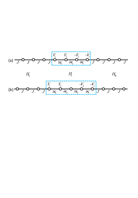
Figure 1: (Color online) Schematic illustration of an anti-$\mathcal{PT}$-symmetric scattering system. The site number of the scattering center is even in (a) and odd in (b).

III Scattering formalism

In this section, we investigate the scattering properties of an anti-$\mathcal{PT}$-symmetric non-Hermitian scattering center, typical scattering behaviors are revealed. In the following, we discuss the scattering properties of the anti-$\mathcal{PT}$-symmetric scattering center through investigating the reflection and transmission of the left and the right inputs. The wave function for the left input is denoted as $\psi_{\mathrm{L}}^{k}\left(j\right)$ and for the right input is denoted as $\psi_{\mathrm{R}}^{k}\left(j\right)$ for site $\left|j\right\rangle_{\mathrm{c}}$, where $k$ is the wave vector. The wave functions are in the form of

$$\psi_{\mathrm{L}}^{k}\left(j\right) = \left\{\begin{array}[]{c}e^{ikj}+r_{\mathrm{L}}e^{-ikj},j<0\\ t_{\mathrm{L}}e^{ikj},j>0\end{array}\right.,$$ (6)

$$\psi_{\mathrm{R}}^{k}\left(j\right) = \left\{\begin{array}[]{c}t_{\mathrm{R}}e^{-ikj},j<0\\ e^{-ikj}+r_{\mathrm{R}}e^{ikj},j>0\end{array}\right..$$ (9)

where $r_{\mathrm{L}}$ ($t_{\mathrm{L}}$) and $r_{\mathrm{R}}$ ($t_{\mathrm{R}}$) are the reflection (transmission) coefficients for the left and right inputs, respectively.

III.1 Identical transmission of transpose invariant

The scattering center satisfies transpose invariant, i.e., $H_{\mathrm{c}}=H_{\mathrm{c}}^{T}$. This leads to identical left and right transmission coefficients, i.e., $t_{\mathrm{L}}=t_{\mathrm{R}}$. For the left input, the Schrödinger equations for the scattering center are in the form of

$$\left(H_{\mathrm{c}}-EI_{N\times N}\right)\Psi_{\mathrm{c,L}}=\Phi_{\mathrm{c,L}},$$ (10)

where $E=2J\cos k$ is the dispersion relation obtained from the Schrödinger equations for the leads; $I_{N\times N}$ is the $N\times N$ dimension identical matrix. $\Psi_{\mathrm{c,L}}$ and $\Phi_{\mathrm{c,L}}$ are $N$ dimension column vectors, their elements are $\Psi_{\mathrm{c,L}}\left(j\right)=\psi_{\mathrm{c}}^{k}\left(j\right)$ for $j\in\left[1,N\right]$. $\psi_{\mathrm{c}}^{k}\left(j\right)$ represents the wave function of site-$j$ in the scattering center $H_{\mathrm{c}}$. $\Phi_{\mathrm{c,L}}\left(1\right)=-g\psi_{\mathrm{L}}^{k}\left(-1\right)$, $\Phi_{\mathrm{c,L}}\left(N\right)=-g\psi_{\mathrm{L}}^{k}\left(+1\right)$, and $\Phi_{\mathrm{c,L}}\left(j\right)=0$ for $j\in\left[2,N-1\right]$. The wave functions at site $\pm 1$ are $\psi_{\mathrm{L}}^{k}\left(-1\right)=e^{-ik}+r_{\mathrm{L}}e^{ik}$ and $\psi_{\mathrm{L}}^{k}\left(+1\right)=t_{\mathrm{L}}e^{ik}$. From Eq. (10), we have

$$\Psi_{\mathrm{c,L}}\left(1\right) = \Delta_{11}^{-1}\Phi_{\mathrm{c,L}}\left(1\right)+\Delta_{1N}^{-1}\Phi_{\mathrm{c,L}}\left(N\right),$$ (11)

$$\Psi_{\mathrm{c,L}}\left(N\right) = \Delta_{N1}^{-1}\Phi_{\mathrm{c,L}}\left(1\right)+\Delta_{NN}^{-1}\Phi_{\mathrm{c,L}}\left(N\right),$$ (12)

where $\Delta=H_{\mathrm{c}}-EI_{N\times N}$, and $\Delta_{mn}^{-1}$ represents the element of matrix $\Delta^{-1}$ on the $m$ row and $n$ column. Then, we have

$$-\frac{\psi_{\mathrm{c}}^{k}\left(1\right)}{g} = \Delta_{11}^{-1}\left(e^{-ik}+r_{\mathrm{L}}e^{ik}\right)+\Delta_{1N}^{-1}t_{\mathrm{L}}e^{ik},$$ (13)

$$-\frac{\psi_{\mathrm{c}}^{k}\left(N\right)}{g} = \Delta_{N1}^{-1}\left(e^{-ik}+r_{\mathrm{L}}e^{ik}\right)+\Delta_{NN}^{-1}t_{\mathrm{L}}e^{ik},$$ (14)

The Schrödinger equations for the lead sites $\left|-1\right\rangle_{\mathrm{l}}$ and $\left|+1\right\rangle_{\mathrm{l}}$ yield

$$J\psi_{\mathrm{L}}^{k}\left(-2\right)+g\psi_{\mathrm{c}}^{k}\left(1\right) = E\psi_{\mathrm{L}}^{k}\left(-1\right),$$ (15)

$$J\psi_{\mathrm{L}}^{k}\left(+2\right)+g\psi_{\mathrm{c}}^{k}\left(N\right) = E\psi_{\mathrm{L}}^{k}\left(1\right),$$ (16)

the wave functions at sites $\pm 2$ are $\psi_{\mathrm{L}}^{k}\left(-2\right)=e^{-2ik}+r_{\mathrm{L}}e^{2ik}$ and $\psi_{\mathrm{L}}^{k}\left(+2\right)=t_{\mathrm{L}}e^{2ik}$. Then, we have

$$\psi_{\mathrm{c}}^{k}\left(1\right)=\frac{J}{g}\left(1+r_{\mathrm{L}}\right),\psi_{\mathrm{c}}^{k}\left(N\right)=\frac{J}{g}t_{\mathrm{L}},$$ (17)

the two kinds of expressions for $\psi_{\mathrm{c}}^{k}\left(1\right)$ and $\psi_{\mathrm{c}}^{k}\left(N\right)$ are equivalent, therefore

$$-\frac{J\left(1+r_{\mathrm{L}}\right)}{g^{2}} = \Delta_{11}^{-1}\left(e^{-ik}+r_{\mathrm{L}}e^{ik}\right)+\Delta_{1N}^{-1}t_{\mathrm{L}}e^{ik},$$ (18)

$$-\frac{J}{g^{2}}t_{\mathrm{L}} = \Delta_{N1}^{-1}\left(e^{-ik}+r_{\mathrm{L}}e^{ik}\right)+\Delta_{NN}^{-1}t_{\mathrm{L}}e^{ik},$$ (19)

and the transmission for the left input is

$$t_{\mathrm{L}}=\frac{2i\left(J/g^{2}\right)\Delta_{N1}^{-1}\sin k}{\left[\frac{J}{g^{2}}+\Delta_{NN}^{-1}e^{ik}\right]\left[\frac{J}{g^{2}}+\Delta_{11}^{-1}e^{ik}\right]-\Delta_{N1}^{-1}\Delta_{1N}^{-1}e^{2ik}}.$$ (20)

For the right input, the Schrödinger equations for the scattering center are in the form of

$$\Delta\Psi_{\mathrm{c,R}}=\Phi_{\mathrm{c,R}},$$ (21)

$\Psi_{\mathrm{c,R}}$ and $\Phi_{\mathrm{c,R}}$ are $N$ dimension column vectors, their elements are $\Psi_{\mathrm{c,R}}\left(j\right)=\psi_{\mathrm{c}}^{k}\left(j\right)$ for $j\in\left[1,N\right]$; $\Phi_{\mathrm{c,R}}\left(1\right)=-g\psi_{\mathrm{R}}^{k}\left(-1\right)$, $\Phi_{\mathrm{c,R}}\left(N\right)=-g\psi_{\mathrm{R}}^{k}\left(+1\right)$, and $\Phi_{\mathrm{c,R}}\left(j\right)=0$ for $j\in\left[2,N-1\right]$. The wave functions at sites $\pm 1$ are $\psi_{\mathrm{R}}^{k}\left(-1\right)=t_{\mathrm{R}}e^{ik}$ and $\psi_{\mathrm{R}}^{k}\left(+1\right)=e^{-ik}+r_{\mathrm{R}}e^{ik}$. From Eq. (10), we have

$$\Psi_{\mathrm{c,R}}\left(1\right) = \Delta_{11}^{-1}\Phi_{\mathrm{c,R}}\left(1\right)+\Delta_{1N}^{-1}\Phi_{\mathrm{c,R}}\left(N\right),$$ (22)

$$\Psi_{\mathrm{c,R}}\left(N\right) = \Delta_{N1}^{-1}\Phi_{\mathrm{c,R}}\left(1\right)+\Delta_{NN}^{-1}\Phi_{\mathrm{c,R}}\left(N\right),$$ (23)

that is

$$-\frac{\psi_{\mathrm{c}}^{k}\left(1\right)}{g} = \Delta_{11}^{-1}t_{\mathrm{L}}e^{ik}+\Delta_{1N}^{-1}\left(e^{-ik}+r_{\mathrm{R}}e^{ik}\right),$$ (24)

$$-\frac{\psi_{\mathrm{c}}^{k}\left(N\right)}{g} = \Delta_{N1}^{-1}t_{\mathrm{L}}e^{ik}+\Delta_{NN}^{-1}\left(e^{-ik}+r_{\mathrm{R}}e^{ik}\right),$$ (25)

The Schrödinger equations for the lead sites $\left|-1\right\rangle_{\mathrm{l}}$ and $\left|+1\right\rangle_{\mathrm{l}}$ yield

$$J\psi_{\mathrm{R}}^{k}\left(-2\right)+g\psi_{\mathrm{c}}^{k}\left(1\right) = E\psi_{\mathrm{R}}^{k}\left(-1\right),$$ (26)

$$J\psi_{\mathrm{R}}^{k}\left(+2\right)+g\psi_{\mathrm{c}}^{k}\left(N\right) = E\psi_{\mathrm{R}}^{k}\left(+1\right),$$ (27)

the wave functions at sites $\pm 2$ are $\psi_{\mathrm{R}}^{k}\left(-2\right)=t_{\mathrm{R}}e^{2ik}$ and $\psi_{\mathrm{R}}^{k}\left(+2\right)=e^{-2ik}+r_{\mathrm{R}}e^{2ik}$. Then, we have

$$\psi_{\mathrm{c}}^{k}\left(1\right)=\frac{J}{g}t_{\mathrm{R}},\psi_{\mathrm{c}}^{k}\left(N\right)=\frac{J}{g}\left(1+r_{\mathrm{R}}\right),$$ (28)

therefore,

$$-\frac{J}{g^{2}}t_{\mathrm{R}} = \Delta_{11}^{-1}t_{\mathrm{L}}e^{ik}+\Delta_{1N}^{-1}\left(e^{-ik}+r_{\mathrm{R}}e^{ik}\right),$$ (29)

$$-\frac{J\left(1+r_{\mathrm{R}}\right)}{g^{2}} = \Delta_{N1}^{-1}t_{\mathrm{L}}e^{ik}+\Delta_{NN}^{-1}\left(e^{-ik}+r_{\mathrm{R}}e^{ik}\right),$$ (30)

and the transmission for the right input is

$$t_{\mathrm{R}}=\frac{2i\left(J/g^{2}\right)\left(\Delta^{-1}\right)_{1N}\sin k}{\left[\frac{J}{g^{2}}+\Delta_{11}^{-1}e^{ik}\right]\left[\frac{J}{g^{2}}+\Delta_{NN}^{-1}e^{ik}\right]-\Delta_{1N}^{-1}\Delta_{N1}^{-1}e^{2ik}}.$$ (31)

Because $H_{\mathrm{c}}=H_{\mathrm{c}}^{T}$, then we have $\Delta=\Delta^{T}$. Notice that $\left(\Delta^{T}\right)^{-1}=\left(\Delta^{-1}\right)^{T}$, then we obtain $\Delta^{-1}=\left(\Delta^{T}\right)^{-1}\Delta^{T}\Delta^{-1}=\left(\Delta^{T}\right)^{-1}=\left(\Delta^{-1}\right)^{T}$. Thus, the matrix elements satisfy $\Delta_{1N}^{-1}=\Delta_{N1}^{-1}$. Through comparing Eqs. (20) and (31), we notice that the left transmission coefficient is identical with the right transmission coefficient. Therefore, the transpose invariant of $H_{\mathrm{c}}$ yields identical transmission coefficients

$$t_{\mathrm{L}}=t_{\mathrm{R}}.$$ (32)

III.2 Reciprocal reflection under $\mathcal{T}$ symmetry

The scattering center is also invariant under time reversal operation. The time reversal operator can be expressed as a unitary operator $\mathcal{U}$ multiples the complex conjugation operator $\mathcal{K}$, i.e., $\mathcal{T}=\mathcal{U}\mathcal{K}$. The element of the unitary operator $\mathcal{U}$ is ${}_{\mathrm{c}}\left\langle m\right|\mathcal{U}\left|n\right\rangle_{\mathrm{c}}=\left(-1\right)^{m-1}\delta\left(m-n\right)$, where $\delta$ is the Dirac delta function.

The unitary operator is a diagonal matrix with staggered elements $+1$ and $-1$, which is a transformation on the scattering center basis. We schematically illustrate this basis transformation in Fig. 2 with the coefficients $+1$ in blue and $-1$ in green. $+1$ indicates that the basis is unchanged; $-1$ indicates that the basis changes from $\left|j\right\rangle_{\mathrm{c}}$ to $-\left|j\right\rangle_{\mathrm{c}}$ after the basis transformation. Figure 2 implies the Hamiltonian of the scattering center $H_{\mathrm{c}}$ is invariant after the time reversal operation, i.e., acting the complex conjugation $\mathcal{K}$ and the basis transformation. To make the whole system Hamiltonian $H$ being invariant after the time reversal operation, the basis on the left and right leads need to change accordingly. The basis on the left lead is unchanged, but changes from $\left|j\right\rangle_{\mathrm{l}}$ to $-\left|j\right\rangle_{\mathrm{l}}$ on the right lead for the scattering center with even-site. To make the whole system Hamiltonian $H$ unchanged after time reversal operation, the coefficients on the basis of the two leads for the scattering center with even-site ($N$ is even) are opposite [Fig. 2(a)]; the basis of the two leads for the scattering center with odd-site ($N$ is odd) is unchanged [Fig. 2(b)]. This difference indicates two distinct relations of the scattering wave functions (Fig. 2). The left input and the right input wave functions with identical wave vector $k$ can compose either the left or the right wave function after time reversal operation in two alternative ways for the scattering center with different parities.

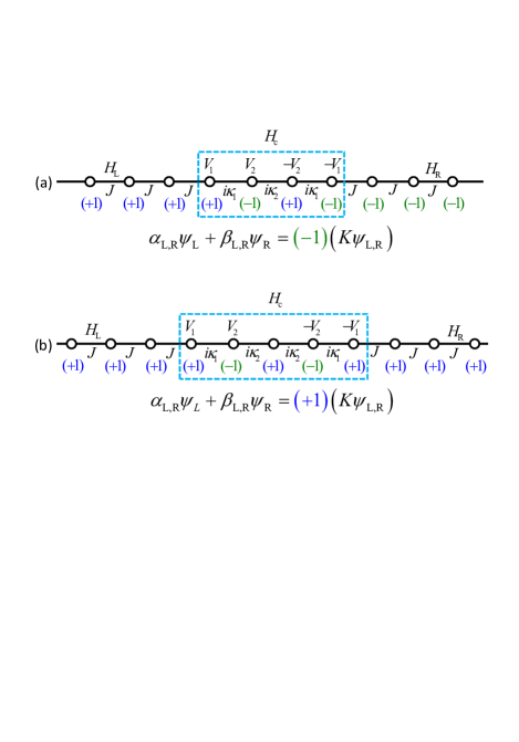
Figure 2: (Color online) The wave function relation between the anti-$\mathcal{PT}$-symmetric scattering system. The site number of the center is (a) even and (b) odd. The $+1$ in blue and $-1$ in green represent the unitary transformation, the scattering system changes back to itself after time reversal operation.

We act the complex conjugation operator $\mathcal{K}$ on the wave functions Eqs. (6,9) to get

$$\mathcal{K}\psi_{\mathrm{L}}^{k}\left(j\right) = \left\{\begin{array}[]{c}e^{-ikj}+r_{\mathrm{L}}^{\ast}e^{ikj},j<0\\ t_{\mathrm{L}}^{\ast}e^{-ikj},j>0\end{array}\right.,$$ (35)

$$\mathcal{K}\psi_{\mathrm{R}}^{k}\left(j\right) = \left\{\begin{array}[]{c}t_{\mathrm{R}}^{\ast}e^{ikj},j<0\\ e^{ikj}+r_{\mathrm{R}}^{\ast}e^{-ikj},j>0\end{array}\right..$$ (38)

For the configuration shown in Fig. 2(a), we can compose $-\mathcal{K}\psi_{\mathrm{L}}^{k}\left(j\right)$ in the $j<0$ region through $\psi_{\mathrm{L}}^{k}\left(j\right)$ and $\psi_{\mathrm{R}}^{k}\left(j\right)$ of Eqs. (6, 9) by eliminating $e^{ikj}$ in $j>0$ region. We have

$$t_{\mathrm{L}}^{\ast}\left[\psi_{\mathrm{R}}^{k}\left(j\right)-\frac{r_{\mathrm{R}}}{t_{\mathrm{L}}}\psi_{\mathrm{L}}^{k}\left(j\right)\right]$$ (41)

$$= \left\{\begin{array}[]{c}t_{\mathrm{L}}^{\ast}\left(t_{\mathrm{R}}-r_{\mathrm{R}}\frac{r_{\mathrm{L}}}{t_{\mathrm{L}}}\right)e^{-ikj}-t_{\mathrm{L}}^{\ast}\frac{r_{\mathrm{R}}}{t_{\mathrm{L}}}e^{ikj},j<0\\ t_{\mathrm{L}}^{\ast}e^{-ikj},j>0\end{array}\right.,$$

the coefficients in $j>0$ region for the composed wave function $t_{\mathrm{L}}^{\ast}\left[\psi_{\mathrm{R}}^{k}\left(j\right)-\frac{r_{\mathrm{R}}}{t_{\mathrm{L}}}\psi_{\mathrm{L}}^{k}\left(j\right)\right]$ and $\mathcal{K}\psi_{\mathrm{L}}^{k}\left(j\right)$ are the same; but they should be opposite in the $j<0$ region. Therefore, the coefficients in the $j<0$ region satisfies

$$t_{\mathrm{L}}^{\ast}\left(t_{\mathrm{R}}-r_{\mathrm{R}}\frac{r_{\mathrm{L}}}{t_{\mathrm{L}}}\right) = -1,$$ (42)

$$-t_{\mathrm{L}}^{\ast}\frac{r_{\mathrm{R}}}{t_{\mathrm{L}}} = -r_{\mathrm{L}}^{\ast},$$ (43)

then we have the relations

$$r_{\mathrm{L}}r_{\mathrm{L}}^{\ast}-t_{\mathrm{L}}^{\ast}t_{\mathrm{R}}=1;t_{\mathrm{L}}^{\ast}r_{\mathrm{R}}=r_{\mathrm{L}}^{\ast}t_{\mathrm{L}},$$ (44)

for the scattering center site number being even.

For the configuration shown in Fig. 2(b), the composed wave function $t_{\mathrm{L}}^{\ast}\left[\psi_{\mathrm{R}}^{k}\left(j\right)-\frac{r_{\mathrm{R}}}{t_{\mathrm{L}}}\psi_{\mathrm{L}}^{k}\left(j\right)\right]$ and $\mathcal{K}\psi_{\mathrm{L}}^{k}\left(j\right)$ are the same in both the left and the right leads. Then, we obtain

$$t_{\mathrm{L}}^{\ast}\left(t_{\mathrm{R}}-r_{\mathrm{R}}\frac{r_{\mathrm{L}}}{t_{\mathrm{L}}}\right) = 1,$$ (45)

$$-t_{\mathrm{L}}^{\ast}\frac{r_{\mathrm{R}}}{t_{\mathrm{L}}} = r_{\mathrm{L}}^{\ast},$$ (46)

and the relations

$$r_{\mathrm{L}}r_{\mathrm{L}}^{\ast}+t_{\mathrm{L}}^{\ast}t_{\mathrm{R}}=1;t_{\mathrm{L}}^{\ast}r_{\mathrm{R}}=-r_{\mathrm{L}}^{\ast}t_{\mathrm{L}},$$ (47)

for the scattering center site number being odd.

For the configuration shown in Fig. 2(a), we compose $-\mathcal{K}\psi_{\mathrm{R}}^{k}\left(j\right)$ via $\psi_{\mathrm{L}}^{k}\left(j\right)$ and $\psi_{\mathrm{R}}^{k}\left(j\right)$ of Eqs. (6, 9) by eliminating $e^{-ikj}$ in $j<0$ region. We have

$$t_{\mathrm{R}}^{\ast}\left[\psi_{\mathrm{L}}^{k}\left(j\right)-\frac{r_{\mathrm{L}}}{t_{\mathrm{R}}}\psi_{\mathrm{R}}^{k}\left(j\right)\right]$$ (50)

$$= \left\{\begin{array}[]{c}t_{\mathrm{R}}^{\ast}e^{ikj},j<0\\ t_{\mathrm{R}}^{\ast}\left(t_{\mathrm{L}}-r_{\mathrm{L}}\frac{r_{\mathrm{R}}}{t_{\mathrm{R}}}\right)e^{ikj}-t_{\mathrm{R}}^{\ast}\frac{r_{\mathrm{L}}}{t_{\mathrm{R}}}e^{-ikj},j>0\end{array}\right.,$$

the coefficients in $j<0$ region for the composed wave function $t_{\mathrm{R}}^{\ast}\left[\psi_{\mathrm{L}}^{k}\left(j\right)-\frac{r_{\mathrm{L}}}{t_{\mathrm{R}}}\psi_{\mathrm{R}}^{k}\left(j\right)\right]$ and $\mathcal{K}\psi_{\mathrm{R}}^{k}\left(j\right)$ are identical; but the coefficients in the $j>0$ region should be opposite. Therefore, we have the relations

$$t_{\mathrm{R}}^{\ast}\left(t_{\mathrm{L}}-r_{\mathrm{L}}\frac{r_{\mathrm{R}}}{t_{\mathrm{R}}}\right) = -1,$$ (51)

$$-t_{\mathrm{R}}^{\ast}\frac{r_{\mathrm{L}}}{t_{\mathrm{R}}} = -r_{\mathrm{R}}^{\ast}.$$ (52)

Simplifying the obtained relations, we have

$$r_{\mathrm{R}}r_{\mathrm{R}}^{\ast}-t_{\mathrm{R}}^{\ast}t_{\mathrm{L}}=1;t_{\mathrm{R}}^{\ast}r_{\mathrm{L}}=r_{\mathrm{R}}^{\ast}t_{\mathrm{R}},$$ (53)

for the scattering center site number being even.

For the configuration shown in Fig. 2(b), the composed wave function $t_{\mathrm{L}}^{\ast}\left[\psi_{\mathrm{R}}^{k}\left(j\right)-\frac{r_{\mathrm{R}}}{t_{\mathrm{L}}}\psi_{\mathrm{L}}^{k}\left(j\right)\right]$ and $\mathcal{K}\psi_{\mathrm{L}}^{k}\left(j\right)$ are the same in both the left and the right leads. Thus, we obtain

$$t_{\mathrm{R}}^{\ast}\left(t_{\mathrm{L}}-r_{\mathrm{L}}\frac{r_{\mathrm{R}}}{t_{\mathrm{R}}}\right) = 1,$$ (54)

$$-t_{\mathrm{R}}^{\ast}\frac{r_{\mathrm{L}}}{t_{\mathrm{R}}} = r_{\mathrm{R}}^{\ast},$$ (55)

after simplification, we obtain the relations

$$r_{\mathrm{R}}r_{\mathrm{R}}^{\ast}+t_{\mathrm{R}}^{\ast}t_{\mathrm{L}}=1;t_{\mathrm{R}}^{\ast}r_{\mathrm{L}}=-t_{\mathrm{R}}r_{\mathrm{R}}^{\ast},$$ (56)

for the scattering center site number being odd.

A direct conclusion from the relations of scattering coefficients Eqs. (44, 53) and Eqs. (47, 56) is the reciprocal reflection, i.e., $\left|r_{\mathrm{L}}\right|=\left|r_{\mathrm{R}}\right|$ in both configurations of Fig. 1.

III.3 Scattering probability and scattering matrix

For the scattering center with even-site, their reflection and transmission satisfy Eqs. (32), (44), and (53), from which we first obtain

$$\left|r_{\mathrm{L}}\right|^{2}-\left|t_{\mathrm{L}}\right|^{2}=\left|r_{\mathrm{R}}\right|^{2}-\left|t_{\mathrm{R}}\right|^{2}=1.$$ (57)

And then, we obtain that the scattering matrix satisfies

$$\left(S\sigma_{\mathrm{z}}\right)\left(S\sigma_{\mathrm{z}}\right)^{\ast}=\left(\begin{array}[]{cc}r_{\mathrm{L}}r_{\mathrm{L}}^{\ast}-t_{\mathrm{R}}t_{\mathrm{R}}^{\ast}&t_{\mathrm{R}}r_{\mathrm{R}}^{\ast}-r_{\mathrm{L}}t_{\mathrm{L}}^{\ast}\\ t_{\mathrm{L}}r_{\mathrm{L}}^{\ast}-r_{\mathrm{R}}t_{\mathrm{R}}^{\ast}&r_{\mathrm{R}}r_{\mathrm{R}}^{\ast}-t_{\mathrm{L}}t_{\mathrm{L}}^{\ast}\end{array}\right)=I_{2\times 2}\text{,}$$ (58)

in the configuration shown in Fig. 2(a), where $S$ is the scattering matrix and $\sigma_{\mathrm{z}}$ is the Pauli matrix defined as

$$S=\left(\begin{array}[]{cc}r_{\mathrm{L}}&t_{\mathrm{R}}\\ t_{\mathrm{L}}&r_{\mathrm{R}}\end{array}\right),\sigma_{\mathrm{z}}=\left(\begin{array}[]{cc}1&0\\ 0&-1\end{array}\right).$$ (59)

For the scattering center with odd-site, their reflection and transmission satisfy Eqs. (32), (47), and (56), from which we first obtain

$$\left|r_{\mathrm{L}}\right|^{2}+\left|t_{\mathrm{L}}\right|^{2}=\left|r_{\mathrm{R}}\right|^{2}+\left|t_{\mathrm{R}}\right|^{2}=1.$$ (60)

And then, we obtain that the scattering matrix is unitary in the configuration shown in Fig. 2(b),

$$SS^{\dagger}=\left(\begin{array}[]{cc}r_{\mathrm{L}}r_{\mathrm{L}}^{\ast}+t_{\mathrm{R}}t_{\mathrm{R}}^{\ast}&r_{\mathrm{L}}t_{\mathrm{L}}^{\ast}+t_{\mathrm{R}}r_{\mathrm{R}}^{\ast}\\ t_{\mathrm{L}}r_{\mathrm{L}}^{\ast}+r_{\mathrm{R}}t_{\mathrm{R}}^{\ast}&t_{\mathrm{L}}t_{\mathrm{L}}^{\ast}+r_{\mathrm{R}}r_{\mathrm{R}}^{\ast}\end{array}\right)=I_{2\times 2}\text{.}$$ (61)

The scattering dynamics exhibited in the odd-site anti-$\mathcal{PT}$-symmetric scattering center is similar as the dynamics in a Hermitian scattering center. Therefore, unitary scattering not only occurs in $\mathcal{PT}$-symmetric non-Hermitian system SChen , but also appears in anti-$\mathcal{PT}$-symmetric non-Hermitian system.

IV Illustrative examples

We consider concrete models to demonstrate our results. The two leads are $H_{\pm}=-\sum_{j=\pm 1}^{\pm\infty}\left|j\pm 1\right\rangle_{\mathrm{ll}}\left\langle j\right|+\mathrm{H.c.}$; the connection Hamiltonian is $H_{\mathrm{in}}=-\left|-1\right\rangle_{\mathrm{lc}}\left\langle 1\right|-\left|2\right\rangle_{\mathrm{cl}}\left\langle+1\right|+\mathrm{H.c.}$; and the Hamiltonian of the two-site scattering center is

$$H_{\mathrm{c}}^{\mathrm{2d}}=\left(\begin{array}[]{cc}V&-i\\ -i&-V\end{array}\right).$$ (62)

The scattering center satisfies $\left(\mathcal{PT}\right)H_{\mathrm{c}}^{\mathrm{2d}}\left(\mathcal{PT}\right)^{-1}=-H_{\mathrm{c}}^{\mathrm{2d}}$. The Schrödinger equations for the scattering center are

$$-\psi_{\mathrm{L(R)}}^{k}\left(-1\right)-i\psi_{\mathrm{c}}^{k}\left(2\right) = \left(E-V\right)\psi_{\mathrm{c}}^{k}\left(1\right),$$ (63)

$$-\psi_{\mathrm{L(R)}}^{k}\left(+1\right)-i\psi_{\mathrm{c}}^{k}\left(1\right) = \left(E+V\right)\psi_{\mathrm{c}}^{k}\left(2\right),$$ (64)

the dispersion is $E=-2\cos k$. For the left input, we set the wave functions as $\psi_{\mathrm{L}}^{k}\left(-1\right)=e^{-ik}+r_{\mathrm{L}}e^{ik}$, $\psi_{\mathrm{c}}^{k}\left(1\right)=1+r_{\mathrm{L}}$, $\psi_{\mathrm{c}}^{k}\left(2\right)=t_{\mathrm{L}}$, and $\psi_{\mathrm{L}}^{k}\left(+1\right)=t_{\mathrm{L}}e^{ik}$. For the right input, we set the wave functions as $\psi_{\mathrm{R}}^{k}\left(-1\right)=t_{\mathrm{R}}e^{ik}$, $\psi_{\mathrm{c}}^{k}\left(1\right)=t_{\mathrm{R}}$, $\psi_{\mathrm{c}}^{k}\left(2\right)=1+r_{\mathrm{R}}$, and $\psi_{\mathrm{R}}^{k}\left(+1\right)=e^{-ik}+r_{\mathrm{R}}e^{ik}$. Substituting the wave functions into the Schrödinger equations, we obtain the reflection and transmission, which read

$$t_{\mathrm{L}} = t_{\mathrm{R}}=\frac{2\sin k}{2\cos ke^{-ik}-V^{2}},$$ (65)

$$r_{\mathrm{L}} = \frac{V^{2}-2+2iV\sin k}{2\cos ke^{-ik}-V^{2}},$$ (66)

$$r_{\mathrm{R}} = \frac{V^{2}-2-2iV\sin k}{2\cos ke^{-ik}-V^{2}}.$$ (67)

Notably, $t_{\mathrm{L}}=t_{\mathrm{R}}$, $\left|r_{\mathrm{L}}\right|=\left|r_{\mathrm{R}}\right|$, and $\left|r_{\mathrm{L}(\mathrm{R})}\right|^{2}-\left|t_{\mathrm{L}(\mathrm{R})}\right|^{2}=1$. The scattering matrix satisfies $(S\sigma_{\mathrm{z}})(S\sigma_{\mathrm{z}})^{\ast}=I$.

For a three-site anti-$\mathcal{PT}$-symmetric scattering center

$$H_{\mathrm{c}}^{\mathrm{3d}}=\left(\begin{array}[]{ccc}V&-i&0\\ -i&0&-i\\ 0&-i&-V\end{array}\right),$$ (68)

we notice that $\left(\mathcal{PT}\right)H_{\mathrm{c}}^{\mathrm{3d}}\left(\mathcal{PT}\right)^{-1}=-H_{\mathrm{c}}^{\mathrm{3d}}$. The connection Hamiltonian is $H_{\mathrm{in}}=-\left|-1\right\rangle_{\mathrm{lc}}\left\langle 1\right|-\left|3\right\rangle_{\mathrm{cl}}\left\langle+1\right|+\mathrm{H.c.}$, and the Schrödinger equations are

$$-\psi_{\mathrm{L(R)}}^{k}\left(-1\right)-i\psi_{\mathrm{c}}^{k}\left(2\right) = \left(E-V\right)\psi_{\mathrm{c}}^{k}\left(1\right),$$ (69)

$$-i\psi_{\mathrm{c}}^{k}\left(1\right)-i\psi_{\mathrm{c}}^{k}\left(3\right) = E\psi_{\mathrm{c}}^{k}\left(2\right),$$ (70)

$$-\psi_{\mathrm{L(R)}}^{k}\left(+1\right)-i\psi_{\mathrm{c}}^{k}\left(2\right) = \left(E+V\right)\psi_{\mathrm{c}}^{k}\left(3\right).$$ (71)

For the left input, the wave functions are set as $\psi_{\mathrm{L}}^{k}\left(-1\right)=e^{-ik}\left(e^{-ik}+r_{\mathrm{L}}e^{ik}\right)$, $\psi_{\mathrm{c}}^{k}\left(1\right)=e^{-ik}\left(1+r_{\mathrm{L}}\right)$, $\psi_{\mathrm{c}}^{k}\left(3\right)=e^{-ik}t_{\mathrm{L}}$, and $\psi_{\mathrm{L}}^{k}\left(+1\right)=t_{\mathrm{L}}$. For the right input, the wave functions are set as $\psi_{\mathrm{R}}^{k}\left(-1\right)=t_{\mathrm{R}}$, $\psi_{\mathrm{c}}^{k}\left(1\right)=e^{-ik}t_{\mathrm{R}}$, $\psi_{\mathrm{c}}^{k}\left(3\right)=e^{-ik}\left(1+r_{\mathrm{R}}\right)$, and $\psi_{\mathrm{R}}^{k}\left(+1\right)=e^{-ik}\left(e^{-ik}+r_{\mathrm{R}}e^{ik}\right)$. After simplification, we obtain the reflection and transmission

$$t_{\mathrm{L}} = t_{\mathrm{R}}=\frac{i\sin k}{\left(e^{-2ik}-V^{2}\right)\cos k+e^{-ik}},$$ (72)

$$r_{\mathrm{L}} = -\frac{\left(e^{ik}+V\right)\left(e^{-ik}-V\right)+1}{\left(e^{-2ik}-V^{2}\right)\cos k+e^{-ik}}\cos k,$$ (73)

$$r_{\mathrm{R}} = -\frac{\left(e^{ik}-V\right)\left(e^{-ik}+V\right)+1}{\left(e^{-2ik}-V^{2}\right)\cos k+e^{-ik}}\cos k.$$ (74)

Thus, $t_{\mathrm{L}}=t_{\mathrm{R}}$, $\left|r_{\mathrm{L}}\right|=\left|r_{\mathrm{R}}\right|$, and $\left|r_{\mathrm{L}(\mathrm{R})}\right|^{2}+\left|t_{\mathrm{L}(\mathrm{R})}\right|^{2}=1$. The scattering matrix is unitary, i.e., $SS^{\dagger}=I$, the scattering dynamics is Hermitian-like.

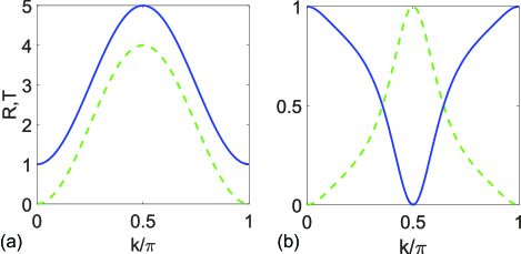
Figure 3: (Color online) The reflection (solid blue) and transmission (dashed green) probabilities as a function of the input wave vector $k$. Plots are for (a) $H_{\mathrm{c}}^{\mathrm{D}}$ and (b) $H_{\mathrm{c}}^{\mathrm{T}}$ at $V=1$.

In Fig. 3, we plot the reciprocal reflection ($R=R_{\mathrm{L}}=R_{\mathrm{R}}$) and reciprocal transmission ($T=T_{\mathrm{L}}=T_{\mathrm{R}}$) probabilities. In Fig. 3(a), $R$ and $T$ are both maximal at $k=\pi/2$, where the input wave has the largest group velocity. The reflection and transmission probabilities monotonously increase as $V$ decreases. Both $R$ and $T$ diverge at $k=\pi/2$ when $V=0$, it corresponds to a spectral singularity and induces symmetric lasing toward both leads AliSS . As $V$ increases, the variations on $R$ and $T$ tend to be flat. In Fig. 3(b), the reflection is zero and the transmission is unity at $k=\pi/2$, which corresponds to a resonant transmission that independent of on-site potentials $V$. As $V$ increases, the variations on $R$ and $T$ around $k=\pi/2$ become sharp. Notably, the spectral singularity can not exist in the discussed anti-$\mathcal{PT}$-symmetric scattering center with site number being odd, where the scattering exhibits Hermitian behavior.

V Summary and Discussion

We have investigated the scattering behavior of an anti-$\mathcal{PT}$-symmetric non-Hermitian scattering center $H_{\mathrm{c}}$ with imaginary nearest-neighbor couplings and real on-site potentials, this type of scattering centers has the feature that $\left(\pm iH_{\mathrm{c}}\right)$ satisfies the $\mathcal{PT}$ symmetry. We find that the reflection ($R$) and transmission ($T$) are both reciprocal; and the probabilities satisfy $R\pm T=1$, which depends on the scattering center size. The scattering matrix of an even-site scattering center satisfies $\left(S\sigma_{\mathrm{z}}\right)\left(S\sigma_{\mathrm{z}}\right)^{\ast}=I$; an odd-site scattering center exhibits Hermitian scattering dynamics, its scattering matrix is unitary $SS^{\dagger}=I$ and none spectral singularity exists. We would like to state that all the conclusions still valid for the scattering center with long range imaginary couplings if all the couplings are between sites with different parity, i.e., only couplings between sites $\left|\mathrm{Odd}\right\rangle_{\mathrm{c}}$ and $\left|\mathrm{Even}\right\rangle_{\mathrm{c}}$ are nonzero; otherwise, only $t_{\mathrm{L}}=t_{\mathrm{R}}$ is valid because of the transpose invariant of the scattering center. Our results are useful in predicting the propagation features of anti-$\mathcal{PT}$-symmetric systems and their applications in optics.

- (1) C. M. Bender, and S. Boettcher, Phys. Rev. Lett. 80, 5243 (1998).
- (2) P. Dorey, C. Dunning, and R. Tateo, J. Phys. A: Math. Gen. 34, L391 (2001).
- (3) A. Mostafazadeh, J. Math. Phys. 43, 3944 (2002).
- (4) W. D. Heiss, J. Phys. A: Math. Gen. 37, 2455 (2004).
- (5) H. F. Jones, J. Phys. A: Math. Gen. 38, 1741 (2005).
- (6) M. Znojil, J. Phys. A: Math. Theor. 41, 292002 (2008).
- (7) K. G. Makris, R. El-Ganainy, D. N. Christodoulides, and Z. H. Musslimani, Phys. Rev. Lett. 100, 103904 (2008).
- (8) S. Klaiman, U. Günther, and N. Moiseyev, Phys. Rev. Lett. 101, 080402 (2008).
- (9) O. Bendix, R. Fleischmann, T. Kottos and B. Shapiro, Phys. Rev. Lett. 103, 030402 (2009).
- (10) L. Jin and Z. Song, Phys. Rev. A 80, 052107 (2009).
- (11) S. Longhi, Phys. Rev. A 82, 031801(R) (2010).
- (12) Y. N. Joglekar, D. Scott, M. Babbey, and A. Saxena, Phys. Rev. A 82, 030103(R) (2010).
- (13) A. Guo, G. J. Salamo, D. Duchesne, R.Morandotti, M. Volatier-Ravat, V. Aimez, G. A. Siviloglou, and D. N. Christodoulides, Phys. Rev. Lett. 103, 093902 (2009).
- (14) C. E. Rüter, K. G. Makris, R. El-Ganainy, D. N. Christodoulides, M. Segev, and D. Kip, Nat. Phys. 6, 192 (2010).
- (15) B. Peng, S. K. Özdemir, F. Lei, F. Monifi, M. Gianfreda, G. L. Long, S. Fan, F. Nori, C. M. Bender, and L. Yang, Nat. Phys. 10, 394 (2014).
- (16) L. Feng, Z. J. Wong, R.-M. Ma, Y. Wang, and X. Zhang, Science 346, 972 (2014).
- (17) H. Hodaei, M.-A. Miri,M. Heinrich, D. N. Christodoulides, and M. Khajavikhan, Science 346, 975 (2014).
- (18) B. Peng, S. K. Özdemira, M. Liertzer, W. Chen, J. Kramer, H. Yılmaz, J. Wiersig, S. Rotter, and L. Yang, Proc. Nat. Acad. Sci. USA 113, 6845 (2016).
- (19) H. Hodaei, A. U. Hassan, S. Wittek, H. Garcia-Gracia, R. El-Ganainy, D. N. Christodoulides, and M. Khajavikhan, Nature 548, 187 (2017).
- (20) W. Chen, S. K. Özdemir, G. Zhao, J. Wiersig, and L. Yang, Nature 548, 192 (2017).
- (21) F. Cannata, J.-P. Dedonder, and A. Ventura, Ann. Phys. (NY) 322, 397 (2007).
- (22) S. Kalish, Z. Lin, and T. Kottos, Phys. Rev. A 85, 055802 (2012).
- (23) Z. Ahmed, Phys. Lett. A 377, 957 (2013).
- (24) A. Mostafazadeh, J. Phys. A: Math. Theor. 47, 505303 (2014).
- (25) B. Zhu, R. Lü, and S. Chen, Phys. Rev. A 91, 042131 (2015).
- (26) X. Q. Li, X. Z. Zhang, G. Zhang, and Z. Song, Phys. Rev. A 91, 032101 (2015).
- (27) L. Jin, X. Z. Zhang, G. Zhang, and Z. Song, Sci. Rep. 6, 20976 (2016).
- (28) Y. D. Chong, Li Ge, Hui Cao and A. D. Stone, Phys. Rev. Lett. 105, 053901 (2010).
- (29) W. Wan, Y. Chong, L. Ge, H. Noh, A. D. Stone, H. Cao, Science 331, 889 (2011).
- (30) Y. Sun, W. Tan, H.-Q. Li, J. Li, H. Chen, Phys. Rev. Lett. 112, 143903 (2014).
- (31) D. G. Baranov, A. Krasnok, T. Shegai, A. Alù, and Y. Chong, Nat. Rev. Mater. 2, 17064 (2017).
- (32) Z. Lin, H. Ramezani, T. Eichelkraut, T. Kottos, H. Cao, and D. N. Christodoulides, Phys. Rev. Lett. 106, 213901 (2011).
- (33) L. Feng, Y. L. Xu, W. S. Fegadolli, M. H. Lu, J. E. B. Oliveira, V. R. Almeida, Y. F. Chen, and A. Scherer, Nat. Mater. 12, 108 (2013).
- (34) R. Fleury, D. Sounas, and A. Alù, Nat. Commun. 6, 5905 (2015).
- (35) H. Ramezani , H. K. Li, Y. Wang, and X. Zhang, Phys. Rev. Lett. 113, 263905 (2014).
- (36) D. A. Antonosyan, A. S. Solntsev, and A. A. Sukhorukov, Opt. Lett. 40, 4575 (2015).
- (37) P. Peng, W. Cao, C. Shen, W. Qu, J. Wen, L. Jiang, and Y. Xiao, Nat. Phys. 12, 1139 (2016).
- (38) L. Ge and H. E. Türeci, Phys. Rev. A 88, 053810 (2013).
- (39) J.-H. Wu, M. Artoni, and G. C. La Rocca, Phys. Rev. Lett. 113, 123004 (2014).
- (40) J.-H. Wu, M. Artoni, and G. C. La Rocca, Phys. Rev. A 91, 033811 (2015).
- (41) V. V. Konotop and D. A. Zezyulin, Phys. Rev. Lett. 120, 123902 (2018).
- (42) A. Mostafazadeh, Phys. Rev. Lett. 102, 220402 (2009).