Stochastic Gravitational-Wave Background from Binary Black Holes and Binary Neutron Stars and Implications for LISA

Abstract

The advent of gravitational wave (GW) and multi-messenger astronomy has stimulated the research on the formation mechanisms of binary black holes (BBHs) observed by LIGO/Virgo. In literature, the progenitors of these BBHs could be stellar-origin black holes (sBHs) or primordial black holes (PBHs). In this paper we calculate the Stochastic Gravitational-Wave Background (SGWB) from BBHs, covering the astrophysical and primordial scenarios separately, together with the one from binary neutron stars (BNSs). Our results indicate that PBHs contribute a stronger SGWB than that from sBHs, and the total SGWB from both BBHs and BNSs has a high possibility to be detected by the future observing runs of LIGO/Virgo and LISA. On the other hand, the SGWB from BBHs and BNSs also contributes an additional source of confusion noise to LISA’s total noise curve, and then weakens LISA’s detection abilities. For instance, the detection of massive black hole binary (MBHB) coalescences is one of the key missions of LISA, and the largest detectable redshift of MBHB mergers can be significantly reduced.

1 Introduction

The detections of gravitational waves (GWs) from binary black hole (BBH) and binary neutron star (BNS) coalescences by LIGO/Virgo (Abbott et al., 2016b, c, e, f, 2017a, 2017b, 2017c, 2017d) have led us to the eras of GW and multi-messenger astronomy. Up to now, there are several BBH merger events reported, of which the masses and redshifts are summarized in Table 1. The progenitors of these BBHs, however, are still under debates. There exist different formation mechanisms in literature to account for the BBHs observed by LIGO/Virgo. Under the assumption that all the BBH mergers are of astrophysical origin, the local merger rate of stellar-mass BBHs is constrained to be $12-213\,\mathrm{Gpc}^{-3}\,\mathrm{yr}^{-1}$ (Abbott et al., 2017b). Besides, the rate of BNS mergers is estimated to be $1540\,^{+3200}_{-1220}\,\mathrm{Gpc}^{-3}\,\mathrm{yr}^{-1}$, utilizing the only so far observed BNS event, GW170817 (Abbott et al., 2017a).

Meanwhile, Table 1 indicates that the masses of BBHs extend over a relatively narrow range around $30M_{\odot}$ with source redshifts $z\lesssim 0.2$, due to the detection ability of current generation of ground-based detectors (the recent LIGO can measure the redshift of BBH mergers up to $z\sim 1$ (Abbott et al., 2016a, 2018b)). Hence, there are many more unresolved BBH merger events, along with other sources, emitting energies, which can be incoherent superposed to constitute a stochastic gravitational-wave background (SGWB) (Christensen, 1992). Different formation channels for BBHs, in general, predict distinct mass and redshift distributions for BBH merger rates, and thus different energy spectra of SGWBs. Therefore, the probing of SGWB may serve as a way to discriminate various formation mechanisms of BBHs.

Assuming all the black holes (BHs) are of stellar origin (Belczynski et al., 2010; Coleman Miller, 2016; Abbott et al., 2016a; Belczynski et al., 2016; Stevenson et al., 2017), the SGWB from BBHs was calculated in  Abbott et al. (2016d, 2017e) and further updated to include BNSs (Abbott et al., 2018a), indicating that this background would likely to be detectable even before reaching LIGO/Virgo’s final design sensitivity, in the most optimistic case. In addition to astrophysical origin, there is another possibility that the detected BBHs are of primordial origin and (partially) play the role of cold dark matter (CDM). In the early Universe, sufficiently dense regions could undergo gravitational collapse by the primordial density inhomogeneity and form primordial black holes (PBHs) (Hawking, 1971; Carr & Hawking, 1974). In literature, two scenarios for PBHs to form BBHs exist (see e.g. García-Bellido (2017) and Sasaki et al. (2018) for recent reviews). The first one is that PBHs in a DM halo interact with each other through gravitational radiation and occasionally bind to form BBHs in the late Universe (Quinlan & Shapiro, 1989; Mouri & Taniguchi, 2002; Bird et al., 2016; Clesse & García-Bellido, 2017a, b). The resulting SGWB for the monochromatic mass function is significantly lower than that from the stellar origin and is unlikely to be measured by LIGO/Virgo (Mandic et al., 2016), while the one for a broad mass function could be potentially enhanced (Clesse & García-Bellido, 2017a). The second one is that two nearby PBHs form a BBH due to the tidal torques from other PBHs in the early Universe (Nakamura et al., 1997; Ioka et al., 1998; Sasaki et al., 2016). The SGWB was investigated in Wang et al. (2018) and Raidal et al. (2017), showing that it is comparable to that from the stellar-origin BBHs (SOBBHs), and could serve as a new probe to constrain the fraction of PBHs in CDM. However, Raidal et al. (2017) only considered the tidal torque due to the nearest PBH, while Wang et al. (2018) assumed that all the PBHs have the same mass.

Events	Primary mass	Secondary mass	Redshift
GW150914	$36.2\,^{+5.2}_{-3.8}$ $M_{\odot}$	$29.1\,^{+3.7}_{-4.4}$ $M_{\odot}$	$0.09\,^{+0.03}_{-0.04}$
LVT151012	$23\,^{+18}_{-6}$ $M_{\odot}$	$13\,^{+4}_{-5}$ $M_{\odot}$	$0.20\,^{+0.09}_{-0.09}$
GW151226	$14.2\,^{+8.3}_{-3.7}$ $M_{\odot}$	$7.5\,^{+2.3}_{-2.3}$ $M_{\odot}$	$0.09\,^{+0.03}_{-0.04}$
GW170104	$31.2\,^{+8.4}_{-6.0}$ $M_{\odot}$	$19.4\,^{+5.3}_{-5.9}$ $M_{\odot}$	$0.18\,^{+0.08}_{-0.07}$
GW170608	$12\,^{+7}_{-2}$ $M_{\odot}$	$7\,^{+2}_{-2}$ $M_{\odot}$	$0.07\,^{+0.03}_{-0.03}$
GW170814	$30.5\,^{+5.7}_{-3.0}$ $M_{\odot}$	$25.3\,^{+2.8}_{-4.2}$ $M_{\odot}$	$0.11\,^{+0.03}_{-0.04}$

Table 1: A summary of the masses and source redshifts of the six BBHs detected by LIGO/Virgo  collaborations  (Abbott et al., 2016f, b, c, b, e, 2017b, 2017c, 2017d).

Recently, the Laser Interferometer Space Antenna (LISA), which aims for a much lower frequency regime, roughly $10^{-4}\sim 10^{-1}\,\mathrm{Hz}$, than that of LIGO/Virgo, has been approved (Audley et al., 2017). In this paper, we will revisit the SGWB produced by BBHs and BNSs, covering both the LIGO/Virgo and LISA frequency band. The impacts of the SGWB on LISA’s detection abilities are also investigated. For sBHs, we adopt the widely accepted “Vangioni” model (Dvorkin et al., 2016) to calculate the corresponding SGWB. For PBHs, we only consider the early Universe scenario. The merger rate for PBHs taking into account the torques by all PBHs and linear density perturbations was considered in Ali-Haïmoud et al. (2017), and later improved to encompass the case with a general mass function for PBHs in Chen & Huang (2018). We will adopt the merger rate presented in Chen & Huang (2018) to estimate the SGWB from primordial-origin BBHs (POBBHs). The rest of this paper is organized as follows. In Sec. 2, assuming all the BBHs are SOBBHs, we calculate the total SGWB from BBH and BNS mergers following Abbott et al. (2018a). In Sec. 3, assuming all the BBHs are POBBHs and using the merger rate density derived in Chen & Huang (2018), we estimate the total SGWB from BBHs and BNSs. Finally, we summarize and discuss our results in Sec. 4

2 SGWB from astrophysical binary black holes and binary neutron stars

There are many different sources in the Universe which can emit GWs at different frequency bands. Among the various sources, BBHs and BNSs are two of the most important ones, which can produce strong SGWB and affect LISA’s detection abilities. In this section, we will focus on the SGWB from SOBBHs and BNSs.

The energy-density spectrum of a GW background can be described by the dimensionless quantity (Allen & Romano, 1999)

$$\Omega_{\mathrm{GW}}(\nu)=\frac{\nu}{\rho_{c}}\frac{\text{d}\rho_{\mathrm{GW}}}{\mathrm{d}\nu},$$ (1)

where $\mathrm{d}\rho_{\mathrm{GW}}$ is the energy density in the frequency interval $\nu$ to $\nu+\mathrm{d}\nu$, $\rho_{c}=3H_{0}^{2}c^{2}/(8\pi G)$ is the critical energy density of the Universe, and $H_{0}=67.74\,\mathrm{km}\,\mathrm{s}^{-1}\,\mathrm{Mpc}^{-1}$ is the Hubble constant taken from Planck (Ade et al., 2016). For the binary mergers, the magnitude of a SGWB can be further transformed to (Phinney, 2001; Regimbau & Mandic, 2008; Zhu et al., 2011, 2013)

$$\begin{split}\Omega_{\mathrm{GW}}(\nu)=&\frac{\nu}{\rho_{c}H_{0}}\int_{0}^{z_{\mathrm{max}}}\mathrm{d}z\int\mathrm{d}m_{1}\mathrm{d}m_{2}\\ &\frac{\mathcal{R}(z,m_{1},m_{2})\frac{\mathrm{d}E_{\mathrm{GW}}}{\mathrm{d}\nu_{s}}(\nu_{s},m_{1},m_{2})}{(1+z)E(\Omega_{r},\Omega_{m},\Omega_{\Lambda},z)},\end{split}$$ (2)

where $\nu_{s}=(1+z)\nu$ is the frequency in source frame, and $E(\Omega_{r},\Omega_{m},\Omega_{\Lambda},z)=\sqrt{\Omega_{r}\left(1+z\right)^{4}+\Omega_{m}(1+z)^{3}+\Omega_{\Lambda}}$ accounts for the dependece of comoving volume on redshift $z$. We adopt the best-fit results from Planck (Ade et al., 2016) that $\Omega_{r}=9.15\times 10^{-5}$, $\Omega_{m}=0.3089$, and $\Omega_{\Lambda}=1-\Omega_{m}-\Omega_{r}$. For the cut-off redshift $z_{\mathrm{max}}$, we choose $z_{\mathrm{max}}=10$ for SOBBHs (Abbott et al., 2016d), and $z_{\mathrm{max}}=\nu_{3}/\nu-1$ for POBBHs (Wang et al., 2018), in which $\nu_{3}$ is given by Eq. (3) below. The energy spectrum emitted by a single BBH $\mathrm{d}E_{\mathrm{GW}}/\mathrm{d}\nu_{s}$ is well approximated by (Cutler et al., 1993; Chernoff & Finn, 1993; Zhu et al., 2011)

$$\frac{\mathrm{d}E_{\mathrm{GW}}}{\mathrm{d}\nu_{s}}=\frac{\left(\pi G\right)^{2/3}M^{5/3}\eta}{3}\begin{cases}\nu_{s}^{-1/3},&\nu_{s}<\nu_{1},\\ \frac{\nu_{s}}{\nu_{1}}\nu^{-1/3},&\nu_{1}\leq\nu_{s}<\nu_{2},\\ \frac{\nu_{s}^{2}}{\nu_{1}\nu_{2}^{4/3}}\frac{\nu_{4}^{4}}{\left(4\left(\nu_{s}-\nu_{2}\right)^{2}+\nu_{4}^{2}\right)^{2}},&\nu_{2}\leq\nu_{s}<\nu_{3},\end{cases}$$ (3)

where $\nu_{i}=\left(a_{i}\eta^{2}+b_{i}\eta+c_{i}\right)/\left(\pi GM/c^{3}\right)$, $M=m_{1}+m_{2}$ is the total mass of the binary, and $\eta=m_{1}m_{2}/M^{2}$. The coefficients $a_{i}$, $b_{i}$ and $c_{i}$ can be found in Table I of Ajith et al. (2008). Since the frequency band of non-zero eccentricity during inspiral phase is below $10^{-4}$ Hz (Dvorkin et al., 2016), which is beyond the frequency range of LISA, we hence only consider the circular orbit during inspiral phase. A careful discussion of the impact of eccentricity on the SGWB can be found in D’Orazio & Samsing (2018).

We will follow the widely accepted “Vangioni” model (Dvorkin et al., 2016) to estimate the SGWB from SOBBHs and BNSs in the Universe. The merger rate density $\mathcal{R}(z,m_{1},m_{2})$ in Eq. (2) for the SOBBHs or BNSs is a convolution of the sBHs or neutron stars (NSs) formation rate $R_{\mathrm{birth}}(z,m_{1})$ with the distribution of the time delays $P_{d}\left(t_{d}\right)$ between the formation and merger of SOBBHs or BNSs,

$$\mathcal{R}=N\int^{t_{\mathrm{max}}}_{t_{\text{min}}}\frac{R_{\mathrm{birth}}(t(z)-t_{d},m_{1})\,\times P_{d}(t_{d})}{\min(m_{1},{m_{\mathrm{max}}}-m_{1})-{m_{\mathrm{min}}}}\ \mathrm{d}t_{d},$$ (4)

where $N$ is a normalization constant, $t(z)$ is the age of the Universe at merger. Here $P_{d}\propto t_{d}^{-1}$ is the distribution of delay time $t_{d}$ with $t_{\mathrm{min}}<t_{d}<t_{\mathrm{max}}$ (Abbott et al., 2018a). The minimum delay time of a massive binary system to evolve until coalescence are set to $t_{\mathrm{min}}=50$ Myr for SOBBHs, and $t_{\mathrm{min}}=20$ Myr for BNSs. Meanwhile, the maximum delay time $t_{\mathrm{max}}$ is set to the Hubble time. In order to comply with the previous studies (Abbott et al., 2017b, 2018a), we restrict the component masses of BBHs to the range ${m_{\mathrm{min}}}\leq m_{2}\leq m_{1}$ and $m_{1}+m_{2}\leq{m_{\mathrm{max}}}$, with ${m_{\mathrm{min}}}=5M_{\odot}$ and ${m_{\mathrm{max}}}=100M_{\odot}$. We note that the merger rate density of POBBHs (see Eq. (12) below) is quite different from Eq. (4), due to the distinct formation mechanisms of POBBHs and SOBBHs.

The most complicated part of Eq. (4) is the computation of the birthrate of sBHs or NSs, which is given by (Dvorkin et al., 2016)

$$\begin{split}R_{\mathrm{birth}}(t,m_{\mathrm{rem}})=&\int\psi[t-\tau(m_{*})]\phi(m_{*})\\ &\delta(m_{*}-g_{\mathrm{rem}}^{-1}(m_{\mathrm{rem}}))\text{d}m_{*},\end{split}$$ (5)

where $m_{*}$ is the mass of the progenitor star, $m_{\mathrm{rem}}$ is the mass of remnant, and $\tau(m_{*})$ is the lifetime of a progenitor star, which can be ignored (Schaerer, 2002). Here $\phi(m_{*})$ is the so called initial mass function (IMF), which is a uniform distribution ranging from $1\,M_{\odot}$ to $2\,M_{\odot}$ for NSs and $\phi(m_{*})\propto m_{*}^{-2.35}$ for sBHs. In addition, $\psi(t)$ is the star formation rate (SFR), which is given by (Nagamine et al., 2004)

$$\psi(z)=k\frac{a\exp[b(z-z_{m})]}{a-b+b\exp[a(z-z_{m})]}.$$ (6)

We will use the fit parameters given by “Fiducial+PopIII” model from Dvorkin et al. (2016), namely, the sum of Fiducial SFR (with $k=0.178\,M_{\odot}\,\mathrm{yr}^{-1}\,\mathrm{Mpc}^{-3}$, $z_{m}=2$, $a=2.37$, $b=1.8$) and PopIII SFR (with $k=0.002\,M_{\odot}\,\mathrm{yr}^{-1}\,\mathrm{Mpc}^{-3}$, $z_{m}=11.87$, $a=13.8$ , $b=13.36$). Dirac delta function in Eq. (5) relates to the process of BH formation. For NSs, $g^{-1}_{\mathrm{ns}}(m_{\mathrm{ns}})=m_{\mathrm{ns}}$, one obtains a relative simple form of birthrate. However, for sBHs, the masses of the progenitor star and the remnant are related by some function $m_{\mathrm{bh}}=g_{\mathrm{bh}}(m_{*})$, which is model-dependent and still unclear yet. In this paper we consider the WWp model (Woosley & Weaver, 1995) of sBH formation, which is simple and indistinguishable from the widely used Fryer model at low redshift (Dvorkin et al., 2016). For progenitor with initial mass $m_{*}$, the mass of the remnant BH $m_{\mathrm{bh}}$ is extrapolated as

$$\frac{m_{\mathrm{bh}}}{m_{*}}=A\left(\frac{m_{*}}{40M_{\odot}}\right)^{\beta}\frac{1}{\left(\frac{Z(z)}{0.01Z_{\odot}}\right)^{\gamma}+1},$$ (7)

where $Z(z)$ is the metallicity and an explicit functional form can be found in Belczynski et al. (2016). The fiducial values of this extrapolation are $A=0.3$, $\beta=0.8$ and $\gamma=0.2$ (Dvorkin et al., 2016). Solving the equation above yields the function $m_{*}=g_{\mathrm{bh}}^{-1}(m_{\mathrm{bh}})$.

Integrating over the component masses in merger rate density, results in the merger rate as a function of redshift

$$\mathcal{R}(z)=\int\mathcal{R}(z,m_{1},m_{2})\,\mathrm{d}m_{1}\text{d}m_{2}.$$ (8)

The local merger rate $R\equiv\mathcal{R}(z=0)$ is inferred to be $R=103_{-63}^{+110}$ $\mathrm{Gpc}^{-3}\,\mathrm{yr}^{-1}$ for SOBBHs (Abbott et al., 2017b), and $R=1540_{-1220}^{+3200}$ $\mathrm{Gpc}^{-3}\,\mathrm{yr}^{-1}$ for BNSs (Abbott et al., 2017a). Utilizing Eq. (2), we then calculate the SGWB from SOBBHs and BNSs. In Fig. 1, we show the corresponding SGWBs as well as the power-law integrated (PI) curves of LIGO (Abbott et al., 2017a) and LISA (Cornish & Robson, 2017, 2018), indicating that the total SGWB from both BBHs and BNSs has a high possibility to be detected by the future observing runs of LIGO/Virgo  and LISA. The energy spectra from both the SOBBHs and BNSs are well approximated by $\Omega_{\mathrm{GW}}\propto\nu^{2/3}$ at low frequencies covering both LISA and LIGO’s bands, where the dominant contribution is from the inspiral phase. We also summarize the background energy densities $\Omega_{\mathrm{GW}}(\nu)$ at the most sensitive frequencies of LIGO (near $25$ Hz) and LISA (near $3\times 10^{-3}$ Hz) in Table 2.

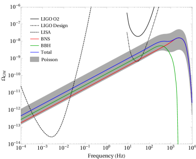
Figure 1: The predicted SGWB from the BNSs and SOBBHs. The red and green curves are backgrounds from the BNSs and BBHs, respectively. The total (BNS and BBH) background is shown in the blue curve, while its Poisson error bars are in the grey shaded region. Here, we adopt the local merger rate $R=103_{-63}^{+110}$ $\mathrm{Gpc}^{-3}\,\mathrm{yr}^{-1}$ for SOBBHs (Abbott et al., 2017b), and $R=1540_{-1220}^{+3200}$ $\mathrm{Gpc}^{-3}\,\mathrm{yr}^{-1}$ for BNSs (Abbott et al., 2017a). We also show the expected PI curves for LISA with $4$ years of observation (dashed) and LIGO’s observing runs of O2 (black) and design sensitivity (dot-dashed). The PI curves for LISA and LIGO’s design sensitivity cross the Poisson error region, indicating the possibility to detect this background.

	$\Omega_{\mathrm{GW}}(25\,\mathrm{Hz})$	$\Omega_{\mathrm{GW}}(3\times 10^{-3}\,\mathrm{Hz})$
BNS	$0.7^{+1.5}_{-0.6}\times 10^{-9}$	$1.7^{+3.5}_{-1.4}\times 10^{-12}$
BBH	$1.1^{+1.2}_{-0.7}\times 10^{-9}$	$2.7^{+2.8}_{-1.6}\times 10^{-12}$
Total	$1.8^{+2.7}_{-1.3}\times 10^{-9}$	$4.4^{+6.3}_{-3.0}\times 10^{-12}$

Table 2: Estimates of the background energy density $\Omega_{\mathrm{GW}}(\nu)$ at the most sensitive frequencies of LIGO (near $25$ Hz) and LISA (near $3\times 10^{-3}$ Hz) for each of the BNS, SOBBH and total background contributions, along with the $90\%$ Poisson error bounds.

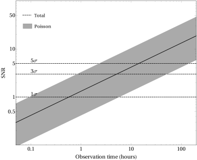
Figure 2: The SNR of LISA as a function of observing time for median total SGWB (black curve) and associated uncertainties (grey shaded region), from the SOBBHs and BNSs. Here, we adopt the local merger rate $R=103_{-63}^{+110}$ $\mathrm{Gpc}^{-3}\,\mathrm{yr}^{-1}$ for SOBBHs (Abbott et al., 2017b), and $R=1540_{-1220}^{+3200}$ $\mathrm{Gpc}^{-3}\,\mathrm{yr}^{-1}$ for BNSs (Abbott et al., 2017a). The predicted median total background can be detected with $\mathrm{SNR}=5$ after about $20$ hours of observation time.

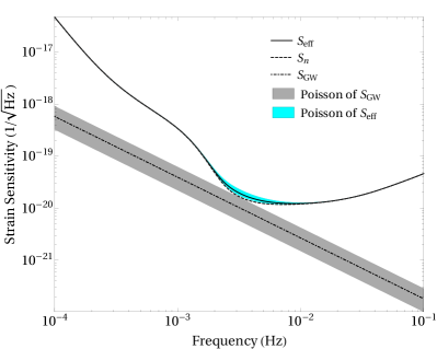
Figure 3: The effective strain sensitivity $S_{\mathrm{eff}}$ (black solid curve) of LISA and its Poisson uncertainties (cyan region), due to the effect of the total SGWB from SOBBHs and BNSs. We also show LISA’s strain sensitivity $S_{n}$ (dashed curve), and $S_{\mathrm{GW}}$ (dot-dashed curve) along with its Poisson uncertainties (grey shaded region).

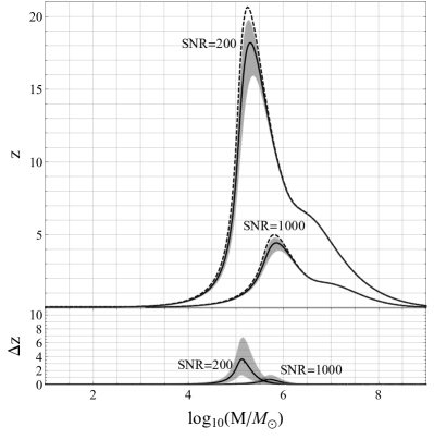
Figure 4: The impacts of the total SGWB from SOBBHs and BNSs on the largest detectable redshift $z$ of MBHB (with total mass $M$) coalescences for LISA. The mass ratio is set to $q=0.2$ following Audley et al. (2017). The upper panel shows the contours of $\mathrm{SNR}=200$ and $\mathrm{SNR}=1000$ for LISA (dashed curves), together with the effect of SGWB (black curves) and the Poisson error bars (grey shaded region). The lower panel shows the residuals of corresponding contours.

The signal-to-noise ratio (SNR) for measuring the SGWB of LISA with observing time $T$ is given by (Thrane & Romano, 2013; Caprini et al., 2016)

$$\text{SNR}=\sqrt{T}\left[\int\mathrm{d}\nu\frac{\Omega_{\mathrm{GW}}(\nu)}{\Omega_{n}(\nu)}\right]^{1/2},$$ (9)

where $\Omega_{n}(\nu)\equiv 2\pi^{2}\nu^{3}S_{n}(\nu)/\left(3H_{0}^{2}\right)$ and $S_{n}$ is the sensitivity of LISA. Fig. 2 shows the expected accumulated SNR of LISA as a function of observation time. The predicted median total background from BBHs and BNSs may be identified with $\mathrm{SNR}=5$ after about $20$ hours of observation. The total background could be identified with $\mathrm{SNR}=5$ within $3$ hours of observation for the most optimistic case, and after about $8$ days for the most pessimistic case.

The total SGWB due to SOBBHs and BNSs is so strong that it may become an unresolved noise, affecting the on-going missions of LISA. For instance, the detection of massive black hole binary (MBHB) coalescences is one of the key missions of LISA (Audley et al., 2017), and the largest detectable redshift of a MBHB merger may be significantly reduced by the additional noise.

Following Barack & Cutler (2004) and Cornish & Robson (2018), we define the noise strain sensitivity due to the SGWB as

$$S_{\mathrm{GW}}(\nu)\equiv\frac{3H_{0}^{2}}{2\pi^{2}}\frac{\Omega_{\mathrm{GW}}(\nu)}{\nu^{3}},$$ (10)

which can be added to the strain sensitivity of LISA $S_{n}(\nu)$ to obtain an effective full strain sensitivity $S_{\mathrm{eff}}(\nu)=S_{n}(\nu)+S_{\mathrm{GW}}(\nu)$. The resulting strain sensitivity curves are shown in Fig. 3. Additionally, the SNR of an single incoming GW strain signal (also called waveform) $h(t)$ has the following form

$$\mathrm{SNR}=2\left[\int\mathrm{d}\nu\frac{|\tilde{h}(\nu)|^{2}}{S_{\mathrm{eff}}(\nu)}\right]^{1/2},$$ (11)

where $\tilde{h}(\nu)$ is the frequency domain representation of $h(t)$, and we adopt the phenomenological waveform provided by Ajith et al. (2008).

Study the growth mechanism of massive black holes (MBHs) is an important science investigation (SI) of LISA (Audley et al., 2017). Among the observational requirements of that SI, being able to measure the dimensionless spin of the largest MBH with an absolute error less than 0.1 and detect the misalignment of spins with the orbital angular momentum better than $10^{\circ}$, requires an accumulated SNR of at least 200. The effect on SNR of MBHB coalescences due to unsolved SGWB signal is shown in Fig. 4, indicating that the largest detectable redshift (with a fixed $\mathrm{SNR}=200$ or $\mathrm{SNR}=1000$) will be reduced. It means that the total detectable region of LISA is suppressed, thus decreasing the event rate of LISA’s scientific missions. Currently, the studies of the origin of MBHs predict that masses of the seeds of MBHs lie in the range about $10^{3}M_{\odot}$ to several $10^{5}M_{\odot}$, with formation redshift around $10\lesssim z\lesssim 15$ (Volonteri, 2010). As shown in Fig. 4, the precise measurement of those seeds above $10^{5}M_{\odot}$ in high formation redshift will be significantly affected by the confusion noise of the unsolved SGWB. Therefore, further analysis is needed to subtract the SGWB signals from the data in order to improve the performance of the detectors.

3 SGWB from binary primordial black holes

In this section, we will calculate the SGWB from PBHs assuming all BHs observed by LIGO/Virgo so far are of primordial origin. Here, we adopt the merger rate for POBBHs presented in Chen & Huang (2018), which takes into account the torques both by all PBHs and linear density perturbations. For a general normalized mass function with parameters $\vec{\theta}$, or the probability distribution function (PDF) for PBHs $P(m|\vec{\theta})$, the comoving merger rate density in units of $\mathrm{Gpc}^{-3}\,\mathrm{yr}^{-1}$ is given by (Chen & Huang, 2018)

$$\mathcal{R}_{12} (t|\vec{\theta})\approx 3.9\cdot 10^{6}\times\left({t\over t_{0}}\right)^{-{34\over 37}}f^{2}(f^{2}+\sigma_{\mathrm{eq}}^{2})^{-{21\over 74}}$$ (12)

$$\times\min\left(\frac{P(m_{1}|\vec{\theta})}{m_{1}},\frac{P(m_{2}|\vec{\theta})}{m_{2}}\right)\left({P(m_{1}|\vec{\theta})\over m_{1}}+{P(m_{2}|\vec{\theta})\over m_{2}}\right)$$

$$\times(m_{1}m_{2})^{{3\over 37}}(m_{1}+m_{2})^{36\over 37},$$

where $t_{0}$ is the age of our Universe, and $\sigma_{\mathrm{eq}}$ is the variance of density perturbations of the rest DM on scale of order ${\cal O}(10^{0}\sim 10^{3})M_{\odot}$ at radiation-matter equality. The component masses of a POBBH, $m_{1}$ and $m_{2}$, are in units of $M_{\odot}$. Similar to Ali-Haïmoud et al. (2017) and Chen & Huang (2018), we take $\sigma_{\mathrm{eq}}\approx 0.005$. Here $f$ is the total abundance of PBHs in non-relativistic matter, and the fraction of PBHs in CDM is related to $f$ by $f_{\mathrm{pbh}}\equiv\Omega_{\mathrm{pbh}}/\Omega_{\mathrm{cdm}}\approx f/0.85$. Integrating over the component masses, yields the merger rate

$$\mathcal{R}(t|\vec{\theta})=\int\mathcal{R}_{12}(t|\vec{\theta})\ \mathrm{d}m_{1}\,\mathrm{d}m_{2},$$ (13)

which is time (or redshift) dependent. The local merger rate density distribution then follows

$$\mathcal{R}_{12}(t_{0}|\vec{\theta})=R\,p(m_{1},m_{2}|\vec{\theta}),$$ (14)

where $p(m_{1},m_{2}|\vec{\theta})$ is the distribution of BH masses in coalescing binaries. The local merger rate $R\equiv\mathcal{R}(t_{0}|\vec{\theta})$ is a normalization constant, such that the population distribution $p(m_{1},m_{2}|\vec{\theta})$ is normalized. Note that all masses are source-frame masses.

We are then interested in extracting the population parameters $\{\vec{\theta},R\}$ from the merger events observed by LIGO/Virgo. This is accomplished by performing the hierarchical Bayesian inference on the BBH’s mass distribution (Abbott et al., 2016h, g, b; Wysocki et al., 2018; Fishbach et al., 2018; Mandel et al., 2018; Thrane & Talbot, 2018). Given the data for $N$ detections, $\vec{d}=(d_{1},\dots,d_{N})$, the likelihood for an inhomogeneous Poisson process, reads (Wysocki et al., 2018; Fishbach et al., 2018; Mandel et al., 2018; Thrane & Talbot, 2018)

$$p(\vec{d}|\vec{\theta},R)\propto R^{N}e^{-R\,\beta(\vec{\theta})}\prod_{i}^{N}\int\mathrm{d}\vec{\lambda}\ p(d_{i}|\vec{\lambda})\ p(\vec{\lambda}|\vec{\theta}),$$ (15)

where $\vec{\lambda}\equiv\{m_{1},m_{2}\}$, and $p(d_{i}|\vec{\lambda})$ is the likelihood of an individual event with data $d_{i}$ given the binary parameters $\vec{\lambda}$. Since the standard priors on masses for each event in LIGO/Virgo analysis are taken to be uniform, one has $p(d_{i}|\vec{\lambda})\propto p(\vec{\lambda}|d_{i})$, and we can use the announced posterior samples (Vallisneri et al., 2015; Abbott et al., 2016b; Biwer et al., 2018) to evaluate the integral in Eq. (15). Meanwhile, $\beta(\vec{\theta})$ is defined as

$$\beta(\vec{\theta})\equiv\int\mathrm{d}\vec{\lambda}\ VT(\vec{\lambda})\ p(\vec{\lambda}|\vec{\theta}),$$ (16)

where $VT(\vec{\lambda})$ is the sensitive spacetime volume of LIGO. We adopt the semi-analytical approximation from Abbott et al. (2016h, g) to calculate $VT$. Specifically, we neglect the effect of spins for BHs, and use aLIGO “Early High Sensitivity” scenario to approximate the power spectral density (PSD) curve. We also consider a single-detector SNR threshold $\rho_{\mathrm{th}}=8$ for detection, which is roughly corresponding to a network threshold of $12$.

The posterior probability function $p(\vec{\theta},R|\vec{d})$ of the population parameters $\{\vec{\theta},R\}$ can be computed by using some assumed prior $p(\vec{\theta},R)$,

$$p(\vec{\theta},R|\vec{d})\propto p(\vec{d}|\vec{\theta},R)\ p(\vec{\theta},R).$$ (17)

We take uniform priors for $\vec{\theta}$ parameters, and a log-uniform one for local merger rate $R$, thus having

$$p(\vec{\theta},R)\propto\frac{1}{R}.$$ (18)

With this prior in hand, the posterior marginalized over $R$ could be easily obtained

$$p(\vec{\theta}|\vec{d})\propto\left[\beta(\vec{\theta})\right]^{-N}\prod_{i}^{N}\int\mathrm{d}\vec{\lambda}\ p(d_{i}|\vec{\lambda})\ p(\vec{\lambda}|\vec{\theta}).$$ (19)

This posterior has been used in previous population inferences (Abbott et al., 2016h, 2017b, b, g; Fishbach & Holz, 2017). We will follow the same procedure as in Abbott et al. (2016h, b, g, 2017b), by first using Eq. (19) to constrain the parameters $\vec{\theta}$, and then fixing $\vec{\theta}$ to their best-fit values in Eq. (17) to infer the local merger rate $R$. As done in the Sec. 2, we also restrict the component masses of BBHs to the range $5M_{\odot}\leq m_{2}\leq m_{1}$ and $m_{1}+m_{2}\leq 100M_{\odot}$. At the time of writing, data analysis for LIGO’s O2 observing run is still on going, we therefore only use the $3$ events from LIGO’s O1 observing run, which contains $48.6$ days of observing time (Abbott et al., 2016b). An update analysis could be performed until the final release of LIGO’s O2 samples. In the following subsections, we will consider two distinct mass functions for PBHs. We will firstly constrain the population parameters $\{\vec{\theta},R\}$ using LIGO’s O1 events, and then calculate the corresponding SGWB from the inferred results.

3.1 Power-law mass function

We now consider a power-law PBH mass functions (Carr, 1975)

$$P(m)\approx{\alpha-1\over M_{\mathrm{min}}}\left({m\over M_{\mathrm{min}}}\right)^{-\alpha},$$ (20)

for $m\geq M_{\mathrm{min}}=5M_{\odot}$ and $\alpha>1$ is the power-law slope. In this case, the free parameters are $\{\vec{\theta},R\}=\{\alpha,R\}$.

Accounting for the selection effects and using $3$ events from LIGO’s O1 run, we find the best-fit result for $\alpha$ is $\alpha=1.61$. Fixing $\alpha$ to this best-fit value, we obtain the median value and $90\%$ equal tailed credible interval for the local merger rate, $R=80\,^{+108}_{-56}$  $\mathrm{Gpc}^{-3}\,\mathrm{yr}^{-1}$. The posterior distributions are shown in Fig. 5. From the posterior distribution of local merger rate $R$, we then infer the fraction of PBHs in CDM $f_{\mathrm{pbh}}=3.8\,^{+2.3}_{-1.8}\times 10^{-3}$. Such an abundance of PBHs is consistent with previous estimations that $10^{-3}\lesssim f_{\mathrm{pbh}}\lesssim 10^{-2}$, confirming that the dominant fraction of CDM should not originate from the stellar mass PBHs (Sasaki et al., 2016; Ali-Haïmoud et al., 2017; Raidal et al., 2017; Kocsis et al., 2018; Chen & Huang, 2018).

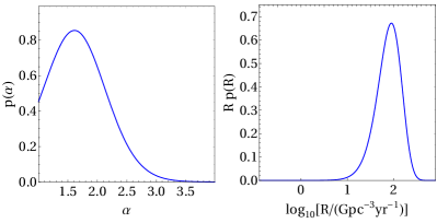
Figure 5: The posterior distributions for $\{\vec{\theta},R\}=\{\alpha,R\}$ for power-law mass function of PBHs, by using $3$ events from LIGO’s O1 observing run.

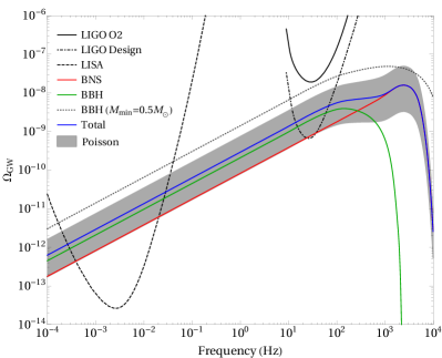
Figure 6: The predicted SGWB from the BNSs and POBBHs with a power-law mass function. The red and green curves are backgrounds from the BNSs and BBHs, respectively. The total (BNS and BBH) background is shown in the blue curve, while its Poisson error bars are in the grey shaded region. For BBHs, we adopt the best-fit value for $\alpha=1.61$, and the inferred local merger rate $R=80\,^{+108}_{-56}$  $\mathrm{Gpc}^{-3}\,\mathrm{yr}^{-1}$, which corresponds to $f_{\mathrm{pbh}}=3.8\,^{+2.3}_{-1.8}\times 10^{-3}$. And for BNSs, we adopt $R=1540_{-1220}^{+3200}$ $\mathrm{Gpc}^{-3}\,\mathrm{yr}^{-1}$ (Abbott et al., 2017a). The dotted line shows the background from BBHs with $M_{\mathrm{min}}=0.5M_{\odot}$, by fixing $\alpha=1.61$ and $R=80$  $\mathrm{Gpc}^{-3}\,\mathrm{yr}^{-1}$. We also show the expected PI curves for LISA with $4$ years of observation (dashed) and LIGO’s observing runs of O2 (black) and design sensitivity (dot-dashed). The PI curves for LISA and LIGO’s design sensitivity cross the Poisson error region, indicating the possibility to detect this background or set upper limits on the population parameters $\{\alpha,R\}$.

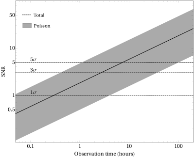
Figure 7: The SNR of LISA as a function of observation time for median total SGWB (black curve) and associated uncertainties (grey shaded region), from the POBBHs (with a power-law mass function) and BNSs. For BBHs, we adopt the best-fit value for $\alpha=1.61$, and the inferred local merger rate $R=80\,^{+108}_{-56}$  $\mathrm{Gpc}^{-3}\,\mathrm{yr}^{-1}$, which corresponds to $f_{\mathrm{pbh}}=3.8\,^{+2.3}_{-1.8}\times 10^{-3}$. And for BNSs, we adopt $R=1540_{-1220}^{+3200}$ $\mathrm{Gpc}^{-3}\,\mathrm{yr}^{-1}$ (Abbott et al., 2017a). The predicted median total background can be detected with $\mathrm{SNR}=5$ after about $10$ hours of observation time.

	$\Omega_{\mathrm{GW}}(25\,\mathrm{Hz})$	$\Omega_{\mathrm{GW}}(3\times 10^{-3}\,\mathrm{Hz})$
BNS	$0.7^{+1.5}_{-0.6}\times 10^{-9}$	$1.7^{+3.5}_{-1.4}\times 10^{-12}$
BBH	$1.8_{-1.3}^{+2.5}\times 10^{-9}$	$4.3^{+5.9}_{-3.0}\times 10^{-12}$
Total	$2.5^{+4.0}_{-1.9}\times 10^{-9}$	$6.0^{+9.4}_{-4.4}\times 10^{-12}$

Table 3: Estimates of the background energy density $\Omega_{\mathrm{GW}}(\nu)$ at the most sensitive frequencies of LIGO (near $25$ Hz) and LISA (near $3\times 10^{-3}$ Hz) for each of the BNS, POBBH (with a power-law PDF) and total background contributions, along with the $90\%$ Poisson error bounds.

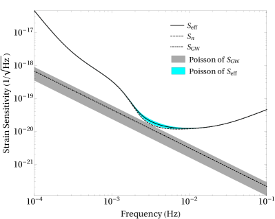
Figure 8: The effective strain sensitivity $S_{\mathrm{eff}}$ (black solid curve) of LISA and its Poisson uncertainties (cyan region), due to the effect of the total SGWB from POBBHs (with a power-law PDF) and BNSs. We also show LISA’s strain sensitivity $S_{n}$ (dashed curve), and $S_{\mathrm{GW}}$ (dot-dashed curve) along with its Poisson uncertainties (grey shaded region).

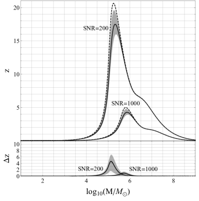
Figure 9: The impacts of the total SGWB from POBBHs (with a power-law PDF) and BNSs, on the largest detectable redshift $z$ of MBHB (with total mass $M$) coalescences for LISA. The mass ratio is set to $q=0.2$ following Audley et al. (2017). The upper panel shows the contours of $\mathrm{SNR}=200$ and $\mathrm{SNR}=1000$ for LISA (dashed curves), together with the effect of SGWB (black curves) and the Poisson error bars (grey shaded region). The lower panel shows the residuals of corresponding contours.

Utilizing Eq. (2), we then calculate the corresponding SGWB. The result is shown in Fig. 6, indicating that the total SGWB from both POBBHs (with a power-law PDF) and BNSs has a high possibility to be detected by the future observing runs of LIGO/Virgo and LISA. In general, a variation of the PBH mass function will affect the profile, e.g. the cutoff frequency and the magnitude, of the energy spectrum $\Omega_{\mathrm{GW}}$. To illustrate this impact, we plot a dotted line in Fig. 6, showing the background with $M_{\mathrm{min}}=0.5M_{\odot}$, by fixing $\{\alpha,R\}$ to their best-fit values as well. The result indicates that the decreasing of $M_{\mathrm{min}}$ will increase the population of the lighter PBHs and hence raise the cutoff frequency. The enhancement of $\Omega_{\mathrm{GW}}$ is mainly due to the extra contribution from the POBBHs with mass range $0.5\sim 5M_{\odot}$. Note that LIGO’s O2 result implies $M_{\mathrm{min}}$ may not be too small; otherwise, SGWB will exceed the upper bround from LIGO’s O2.

The energy spectra from both the POBBHs (with a power-law PDF) and BNSs are well approximated by $\Omega_{\mathrm{GW}}\propto\nu^{2/3}$ at low frequencies covering both LISA and LIGO’s bands, where the dominant contribution is from the inspiral phase. We also summarize the background energy densities $\Omega_{\mathrm{GW}}(\nu)$ at the most sensitive frequencies of LIGO (near $25$ Hz) and LISA (near $3\times 10^{-3}$ Hz) in Table 3.

Fig. 7 shows the expected accumulated SNR of LISA as a function of observing time. The predicted median total background from POBBHs (with a power-law PDF) and BNSs may be identified with $\mathrm{SNR}=5$ after about $10$ hours of observation. The total background could be identified with $\mathrm{SNR}=5$ within $2$ hours of observation for the most optimistic case, and after about $5$ days for the most pessimistic case. The strain sensitivity curves for LISA are shown in Fig. 8. The effect on SNR of MBHB coalescences due to the unsolved SGWB signal is shown in Fig. 9, indicating the precise measurement of the seeds of MBHs above $10^{5}M_{\odot}$ in high formation redshift will be significantly affected by the confusion noise of the unsolved SGWB.

3.2 Lognormal mass function

We now consider another mass distribution, which has a lognormal form (Dolgov & Silk, 1993),

$$P(m)=\frac{1}{\sqrt{2\pi}\sigma m}\exp\left(-\frac{\ln^{2}(m/m_{c})}{2\sigma^{2}}\right),$$ (21)

where $m_{c}$ and $\sigma$ give the peak mass of $mP(m)$ and the width of mass spectrum, respectively. In this model, the free parameters are $\{\vec{\theta},R\}=\{m_{c},\sigma,R\}$.

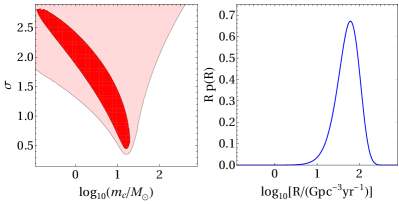
Figure 10: The posterior distributions for $\{\vec{\theta},R\}=\{m_{c},\sigma,R\}$ of lognormal mass function for PBHs, at the $68\%$ and $95\%$ credible level, respectively, by using $3$ events from LIGO’s O1 observing run.

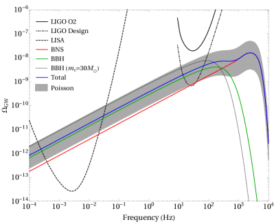
Figure 11: The predicted SGWB from the BNSs and POBBHs with a lognormal mass function. The red and green curves are backgrounds from the BNSs and BBHs, respectively. The total (BNS and BBH) background is shown in the blue curve, while its Poisson error bars are in the grey shaded region. For BBHs, we adopt the best-fit values for $\{m_{c},\sigma\}=\{14.8\,M_{\odot},\,0.65\}$, and the inferred local merger rate $R=55\,^{+74}_{-38}$  $\mathrm{Gpc}^{-3}\,\mathrm{yr}^{-1}$, which corresponds to $f_{\mathrm{pbh}}=2.8\,^{+1.6}_{-1.3}\times 10^{-3}$. And for BNSs, we adopt $R=1540_{-1220}^{+3200}$ $\mathrm{Gpc}^{-3}\,\mathrm{yr}^{-1}$ (Abbott et al., 2017a). The dotted line shows the background from BBHs with $m_{c}=30M_{\odot}$, by fixing $\sigma=0.65$ and $R=55$  $\mathrm{Gpc}^{-3}\,\mathrm{yr}^{-1}$. We also show the expected PI curves for LISA with $4$ years of observation (dashed) and LIGO’s observing runs of O2 (black) and design sensitivity (dot-dashed). The PI curves for LISA and LIGO’s design sensitivity cross the Poisson error region, indicating the possibility to detect this background or set upper limits on the population parameters $\{m_{c},\sigma,R\}$.

	$\Omega_{\mathrm{GW}}(25\,\mathrm{Hz})$	$\Omega_{\mathrm{GW}}(3\times 10^{-3}\,\mathrm{Hz})$
BNS	$0.7^{+1.5}_{-0.6}\times 10^{-9}$	$1.7^{+3.5}_{-1.4}\times 10^{-12}$
BBH	$2.0^{+2.7}_{-1.4}\times 10^{-9}$	$6.3^{+8.5}_{-4.2}\times 10^{-12}$
Total	$2.7^{+4.2}_{-2.0}\times 10^{-9}$	$8.0^{+12}_{-5.6}\times 10^{-12}$

Table 4: Estimates of the background energy density $\Omega_{\mathrm{GW}}(\nu)$ at the most sensitive frequencies of LIGO (near $25$ Hz) and LISA (near $3\times 10^{-3}$ Hz) for each of the BNS, POBBH (with a lognormal PDF) and total background contributions, along with the $90\%$ Poisson error bounds.

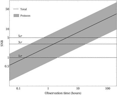
Figure 12: The SNR of LISA as a function of observation time for median total SGWB (black curve) and associated uncertainties (grey shaded region), from POBBHs (with a lognormal mass function) and BNSs. Here, we adopt the best-fit values for $\{m_{c},\sigma\}=\{14.8\,M_{\odot},\,0.65\}$, and the inferred local merger rate $R=55\,^{+74}_{-38}$  $\mathrm{Gpc}^{-3}\,\mathrm{yr}^{-1}$, which corresponds to $f_{\mathrm{pbh}}=2.8\,^{+1.6}_{-1.3}\times 10^{-3}$. The predicted median total background can be detected with $\mathrm{SNR}=5$ after about $5$ hours of observation time.

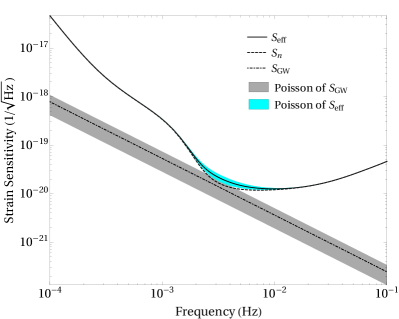
Figure 13: The effective strain sensitivity $S_{\mathrm{eff}}$ (black solid curve) of LISA and its Poisson uncertainties (cyan region), due to the effect of the total SGWB from POBBHs (with a log-normal PDF) and BNSs. We also show LISA’s strain sensitivity $S_{n}$ (dashed curve), and $S_{\mathrm{GW}}$ (dot-dashed curve) along with its Poisson uncertainties (grey shaded region).

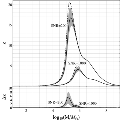
Figure 14: The impacts of the total SGWB from POBBHs (with a lognormal PDF) and BNSs, on the largest detectable redshift $z$ of MBHB (with total mass $M$) coalescences for LISA. The mass ratio is set to $q=0.2$ following Audley et al. (2017). The upper panel shows the contours of $\mathrm{SNR}=200$ and $\mathrm{SNR}=1000$ for LISA (dashed curves), together with the effect of SGWB (black curves) and the Poisson error bars (grey shaded region). The lower panel shows the residuals of corresponding contours.

Accounting for the selection effects and using $3$ events from LIGO’s O1 run, we find the best-fit results for $\vec{\theta}$ are $\{m_{c},\sigma\}=\{14.8\,M_{\odot},\,0.65\}$. Fixing $\vec{\theta}$ to their best-fit values, we obtain the median value and $90\%$ equal tailed credible interval for the local merger rate, $R=55\,^{+74}_{-38}$  $\mathrm{Gpc}^{-3}\,\mathrm{yr}^{-1}$. From the posterior distribution of local merger rate $R$, we then infer the fraction of PBHs in CDM $f_{\mathrm{pbh}}=2.8\,^{+1.6}_{-1.3}\times 10^{-3}$. Such an abundance of PBHs is consistent with previous estimations that $10^{-3}\lesssim f_{\mathrm{pbh}}\lesssim 10^{-2}$, confirming that the dominant fraction of CDM should not originate from the stellar mass PBHs (Sasaki et al., 2016; Ali-Haïmoud et al., 2017; Raidal et al., 2017; Kocsis et al., 2018; Chen & Huang, 2018). The posterior distributions are shown in Fig. 10. Compared to the results given in Raidal et al. (2017), we see that, with the sensitivity of LIGO considered, a more restrictive constrains on the PDFs could be achieved.

Utilizing Eq. (2), we then calculate the corresponding SGWB. The result is shown in Fig. 11, indicating that the total SGWB from both POBBHs (with a lognormal PDF) and BNSs has a high possibility to be detected by the future observing runs of LIGO/Virgo and LISA. To illustrate the impact of mass function on the profile of $\Omega_{\mathrm{GW}}$, we also plot a dotted line in Fig. 11, showing the background with $m_{c}=30M_{\odot}$, by fixing $\{\sigma,R\}$ to their best-fit values. The result indicates that the shifting of the central mass $m_{c}$ to a larger value will decrease the cutoff frequency and increase the magnitude of $\Omega_{\mathrm{GW}}$, and vise versa.

The SGWB for the lognormal mass function was earlier calculated in Raidal et al. (2017) (see Fig. 2 therein). They obtain a larger $\Omega_{\mathrm{GW}}$ than ours, indicating LIGO’s O1 and O2 have the possibility to detect the SGWB from POBBHs. There are a few reasons for this discrepancy. Firstly, Raidal et al. (2017) inferred the parameters of the lognormal PDF by fitting the mass function instead of the merger rate distribution with LIGO’s events and estimate the sensitivity of LIGO by restricting the mass range to $7\sim 50M_{\odot}$. Here, we should note that the events of LIGO may not represent the intrinsic mass function due to the selection bias, of which the impact was ignored by Raidal et al. (2017). Their best-fits are $\{m_{c},\sigma\}=\{33\,M_{\odot},\,0.8\}$, which is quite different from ours. Secondly, Raidal et al. (2017) used the local merger rate $12\sim 213$  $\mathrm{Gpc}^{-3}\,\mathrm{yr}^{-1}$ derived from SOBBHs (Abbott et al., 2017b), although which might serve as a good conservative estimation, to infer the fraction of PBHs $f_{\mathrm{pbh}}$. In this paper, however, we improve their results by fitting the merger rate distribution using a full hierarchical Bayesian analysis, and obtain $R=55\,^{+74}_{-38}$  $\mathrm{Gpc}^{-3}\,\mathrm{yr}^{-1}$ for POBBHs.

The energy spectra from both the POBBHs (with a lognormal PDF) and BNSs are well approximated by $\Omega_{\mathrm{GW}}\propto\nu^{2/3}$ at low frequencies covering both LISA and LIGO’s bands, where the dominant contribution is from the inspiral phase. We also summarize the background energy densities $\Omega_{\mathrm{GW}}(\nu)$ at the most sensitive frequencies of LIGO (near $25$ Hz) and LISA (near $3\times 10^{-3}$ Hz) in Table 4.

Fig. 12 shows the expected accumulated SNR of LISA as a function of observing time. The predicted median total background from POBBHs (with a lognormal PDF) and BNSs may be identified with $\mathrm{SNR}=5$ after about $5$ hours of observation. The total background could be identified with $\mathrm{SNR}=5$ within $1$ hours of observation for the most optimistic case, and after about $3$ days for the most pessimistic case. The strain sensitivity curves for LISA are shown in Fig. 13. The effect on SNR of MBHB coalescences due to unsolved SGWB signal is shown in Fig. 14, indicating the precise measurement of the seeds of MBHs above $10^{5}M_{\odot}$ in high formation redshift will be significantly affected by the confusion noise of the unsolved SGWB.

4 Summary and Discussion

In this paper, we compute the total SGWB arising from both the BBH and BNS mergers. The influences of this SGWB on LISA’s detection abilities is also investigated. Two mechanisms for BBH formation, the astrophysical and primordial origins, are considered separately.

For sBHs, we adopt the widely accepted “Vangioni” model (Dvorkin et al., 2016). For the PBHs, we consider two popular but distinctive mass functions, the power-law and lognormal PDFs, respectively. For the power-law case, we infer the local merger rate to be $R=80\,^{+108}_{-56}$  $\mathrm{Gpc}^{-3}\,\mathrm{yr}^{-1}$, which corresponds to $f_{\mathrm{pbh}}=3.8\,^{+2.3}_{-1.8}\times 10^{-3}$; while for the lognormal case, $R=55\,^{+74}_{-38}$  $\mathrm{Gpc}^{-3}\,\mathrm{yr}^{-1}$ and $f_{\mathrm{pbh}}=2.8\,^{+1.6}_{-1.3}\times 10^{-3}$. Comparing to the lognormal mass function, the power-law one implies a relatively lighter BBH mass distribution and is compensated by a larger local merger rate, for consistency with the event rate of LIGO/Virgo. Note that for both PDFs of PBHs, the inferred abundance of PBHs $f_{\mathrm{pbh}}$ is consistent with previous estimations that $10^{-3}\lesssim f_{\mathrm{pbh}}\lesssim 10^{-2}$, confirming that the dominant fraction of CDM should not originate from the stellar mass PBHs (Sasaki et al., 2016; Ali-Haïmoud et al., 2017; Raidal et al., 2017; Kocsis et al., 2018; Chen & Huang, 2018).

The resulting amplitude of SGWB from PBHs is significantly overall larger than the previous estimation in Mandic et al. (2016), which adopted the late Universe scenario and assumed all the PBHs are of the same mass. There are two reasons to account for this discrepancy. One is that the early Universe scenario predicts much larger local merger rate than the late Universe case ($R=16\,\mathrm{Gpc}^{-3}\,\mathrm{yr}^{-1}$ in Mandic et al. (2016)). Another one is that the merger rate (see Eq. (12)) of the early Universe model is strongly dependent on the redshift and sharply increase with redshift. However, the merger rate of the late Universe model is weakly dependent on redshift and slightly increases with redshift. We refer to Mandic et al. (2016) for more details on the late Universe model. We should emphasize that the above discussion applies only to the late Universe scenario with a monochromatic mass function. For the late Universe scenario with a general mass function, the merger rate could be significantly enhanced and the amplitude of SGWB could be greatly increased (Clesse & García-Bellido, 2017a).

Furthermore, PBHs contribute a stronger (at least comparable if we consider the uncertainties on the formation models of sBHs) SGWB than that from the sBHs (see Figs. 1, 6, 11, and also Tables 2, 3, 4). This is due to that the merger rate densities from PBHs and sBHs have quite different dependences on the BH masses and redshift. Especially, the merger rate of PBHs sharply increases with redshift; while the merger rate of sBHs first increases, then peaks around $z\sim 1-2$, and last rapidly decreases with redshift.

In addition, the background energy densities from primordial and astrophysical BBH mechanisms, both show no clear deviation from the power law spectrum $\Omega_{\mathrm{GW}}\propto\nu^{2/3}$, within LIGO/Virgo and LISA sensitivity band. Thanks to their similar effects on the spectra, distinguishing the backgrounds between POBBHs (the early Universe scenario) and SOBBHs will be challenging. However, Clesse & García-Bellido (2017a) claimed that the SGWB of POBBHs from the late Universe could potentially deviate $\Omega_{\mathrm{GW}}\propto\nu^{2/3}$ at the pulsar timing arrays (PTA) frequencies and even at the frequencies higher enough to be probed by LISA. The feature presented in Clesse & García-Bellido (2017a) may be used to distinguish different formation channels of BBHs.

Finally, the total SGWB from both BBHs (whether astrophysical or primordial origin) and BNSs has a high possibility to be detected by the future observing runs of LIGO/Virgo  and LISA, as could be seen from Figs. 1, 2, 6, 7, 11, 12. This SGWB also contributes an additional source of confusion noise to LISA’s total noise curve (see Figs. 3, 8, 13), and hence weakens LISA’s detection abilities. For instance, the detection of MBHB coalescences is one of the key missions of LISA, and the largest detectable redshift of MBHB mergers can be significantly reduced (see Figs. 4, 9, 14). Therefore, further analysis is needed to subtract the SGWB signals from the data in order to improve the performance of the detectors.

References

- Abbott et al. (2017a) Abbott, B., et al. 2017a, Phys. Rev. Lett., 119, 161101
- Abbott et al. (2016a) Abbott, B. P., et al. 2016a, Astrophys. J., 818, L22
- Abbott et al. (2016b) —. 2016b, Phys. Rev., X6, 041015
- Abbott et al. (2016c) —. 2016c, Phys. Rev., D93, 122003
- Abbott et al. (2016d) —. 2016d, Phys. Rev. Lett., 116, 131102
- Abbott et al. (2016e) —. 2016e, Phys. Rev. Lett., 116, 241103
- Abbott et al. (2016f) —. 2016f, Phys. Rev. Lett., 116, 061102
- Abbott et al. (2016g) —. 2016g, Astrophys. J. Suppl., 227, 14
- Abbott et al. (2016h) —. 2016h, Astrophys. J., 833, L1
- Abbott et al. (2017b) —. 2017b, Phys. Rev. Lett., 118, 221101
- Abbott et al. (2017c) —. 2017c, Astrophys. J., 851, L35
- Abbott et al. (2017d) —. 2017d, Phys. Rev. Lett., 119, 141101
- Abbott et al. (2017e) —. 2017e, Phys. Rev. Lett., 118, 121101, [Erratum: Phys. Rev. Lett.119,no.2,029901(2017)]
- Abbott et al. (2018a) —. 2018a, Phys. Rev. Lett., 120, 091101
- Abbott et al. (2018b) —. 2018b, Living Rev. Rel., 21, 3
- Ade et al. (2016) Ade, P. A. R., et al. 2016, Astron. Astrophys., 594, A13
- Ajith et al. (2008) Ajith, P., et al. 2008, Phys. Rev., D77, 104017, [Erratum: Phys. Rev.D79,129901(2009)]
- Ali-Haïmoud et al. (2017) Ali-Haïmoud, Y., Kovetz, E. D., & Kamionkowski, M. 2017, Phys. Rev., D96, 123523
- Allen & Romano (1999) Allen, B., & Romano, J. D. 1999, Phys. Rev., D59, 102001
- Audley et al. (2017) Audley, H., et al. 2017, arXiv:1702.00786 [astro-ph.IM]
- Barack & Cutler (2004) Barack, L., & Cutler, C. 2004, Phys. Rev., D70, 122002
- Belczynski et al. (2010) Belczynski, K., Dominik, M., Bulik, T., et al. 2010, Astrophys. J., 715, L138
- Belczynski et al. (2016) Belczynski, K., Holz, D. E., Bulik, T., & O’Shaughnessy, R. 2016, Nature, 534, 512
- Bird et al. (2016) Bird, S., Cholis, I., Muñoz, J. B., et al. 2016, Phys. Rev. Lett., 116, 201301
- Biwer et al. (2018) Biwer, C. M., Capano, C. D., De, S., et al. 2018, arXiv:1807.10312 [astro-ph.IM]
- Caprini et al. (2016) Caprini, C., et al. 2016, JCAP, 1604, 001
- Carr (1975) Carr, B. J. 1975, Astrophys. J., 201, 1
- Carr & Hawking (1974) Carr, B. J., & Hawking, S. W. 1974, Mon. Not. Roy. Astron. Soc., 168, 399
- Chen & Huang (2018) Chen, Z.-C., & Huang, Q.-G. 2018, Astrophys. J., 864, 61
- Chernoff & Finn (1993) Chernoff, D. F., & Finn, L. S. 1993, Astrophys. J., 411, L5
- Christensen (1992) Christensen, N. 1992, Phys. Rev., D46, 5250
- Clesse & García-Bellido (2017a) Clesse, S., & García-Bellido, J. 2017a, Phys. Dark Univ., 18, 105
- Clesse & García-Bellido (2017b) —. 2017b, Phys. Dark Univ., 15, 142
- Coleman Miller (2016) Coleman Miller, M. 2016, Gen. Rel. Grav., 48, 95
- Cornish & Robson (2017) Cornish, N., & Robson, T. 2017, J. Phys. Conf. Ser., 840, 012024
- Cornish & Robson (2018) —. 2018, arXiv:1803.01944 [astro-ph.HE]
- Cutler et al. (1993) Cutler, C., Poisson, E., Sussman, G. J., & Finn, L. S. 1993, Phys. Rev., D47, 1511
- Dolgov & Silk (1993) Dolgov, A., & Silk, J. 1993, Phys. Rev., D47, 4244
- D’Orazio & Samsing (2018) D’Orazio, D. J., & Samsing, J. 2018
- Dvorkin et al. (2016) Dvorkin, I., Vangioni, E., Silk, J., Uzan, J.-P., & Olive, K. A. 2016, Mon. Not. Roy. Astron. Soc., 461, 3877
- Fishbach & Holz (2017) Fishbach, M., & Holz, D. E. 2017, Astrophys. J., 851, L25
- Fishbach et al. (2018) Fishbach, M., Holz, D. E., & Farr, W. M. 2018, Astrophys. J., 863, L41, [Astrophys. J. Lett.863,L41(2018)]
- García-Bellido (2017) García-Bellido, J. 2017, J. Phys. Conf. Ser., 840, 012032
- Hawking (1971) Hawking, S. 1971, Mon. Not. Roy. Astron. Soc., 152, 75
- Ioka et al. (1998) Ioka, K., Chiba, T., Tanaka, T., & Nakamura, T. 1998, Phys. Rev., D58, 063003
- Kocsis et al. (2018) Kocsis, B., Suyama, T., Tanaka, T., & Yokoyama, S. 2018, Astrophys. J., 854, 41
- Mandel et al. (2018) Mandel, I., Farr, W. M., & Gair, J. R. 2018, arXiv:1809.02063 [physics.data-an]
- Mandic et al. (2016) Mandic, V., Bird, S., & Cholis, I. 2016, Phys. Rev. Lett., 117, 201102
- Mouri & Taniguchi (2002) Mouri, H., & Taniguchi, Y. 2002, Astrophys. J., 566, L17
- Nagamine et al. (2004) Nagamine, K., Springel, V., & Hernquist, L. 2004, Mon. Not. Roy. Astron. Soc., 348, 421
- Nakamura et al. (1997) Nakamura, T., Sasaki, M., Tanaka, T., & Thorne, K. S. 1997, Astrophys. J., 487, L139
- Phinney (2001) Phinney, E. S. 2001, astro-ph/0108028
- Quinlan & Shapiro (1989) Quinlan, G. D., & Shapiro, S. L. 1989, ApJ, 343, 725
- Raidal et al. (2017) Raidal, M., Vaskonen, V., & Veermäe, H. 2017, JCAP, 1709, 037
- Regimbau & Mandic (2008) Regimbau, T., & Mandic, V. 2008, Class. Quant. Grav., 25, 184018
- Sasaki et al. (2016) Sasaki, M., Suyama, T., Tanaka, T., & Yokoyama, S. 2016, Phys. Rev. Lett., 117, 061101
- Sasaki et al. (2018) —. 2018, Class. Quant. Grav., 35, 063001
- Schaerer (2002) Schaerer, D. 2002, Astron. Astrophys., 382, 28
- Stevenson et al. (2017) Stevenson, S., Vigna-Gómez, A., Mandel, I., et al. 2017, Nature Commun., 8, 14906
- Thrane & Romano (2013) Thrane, E., & Romano, J. D. 2013, Phys. Rev., D88, 124032
- Thrane & Talbot (2018) Thrane, E., & Talbot, C. 2018, arXiv:1809.02293 [astro-ph.IM]
- Vallisneri et al. (2015) Vallisneri, M., Kanner, J., Williams, R., Weinstein, A., & Stephens, B. 2015, J. Phys. Conf. Ser., 610, 012021
- Volonteri (2010) Volonteri, M. 2010, Astron. Astrophys. Rev., 18, 279
- Wang et al. (2018) Wang, S., Wang, Y.-F., Huang, Q.-G., & Li, T. G. F. 2018, Phys. Rev. Lett., 120, 191102
- Woosley & Weaver (1995) Woosley, S. E., & Weaver, T. A. 1995, Astrophys. J. Suppl., 101, 181
- Wysocki et al. (2018) Wysocki, D., Lange, J., & O. ’shaughnessy, R. 2018, arXiv:1805.06442 [gr-qc]
- Zhu et al. (2011) Zhu, X.-J., Howell, E., Regimbau, T., Blair, D., & Zhu, Z.-H. 2011, Astrophys. J., 739, 86
- Zhu et al. (2013) Zhu, X.-J., Howell, E. J., Blair, D. G., & Zhu, Z.-H. 2013, Mon. Not. Roy. Astron. Soc., 431, 882