The composite operator method route to the 2D Hubbard model and the cuprates

Abstract

In this review paper, we illustrate a possible route to obtain a reliable solution of the 2D Hubbard model and an explanation for some of the unconventional behaviours of underdoped high-$T_{\text{c}}$ cuprate superconductors within the framework of the composite operator method. The latter is described exhaustively in its fundamental philosophy, various ingredients and robust machinery to clarify the reasons behind its successful applications to many diverse strongly correlated systems, controversial phenomenologies and puzzling materials.

Key words: many-body techniques, strongly correlated systems, Hubbard model, cuprates, pseudogap, electronic structure

PACS: 71.10.−w, 71.10.Fd, 71.27.+a, 71.18.+y, 74.72.−h, 79.60.−i

Abstract

Ó öié îãëÿäîâié ñòàòòi ìè ïîêàçóєìî ìîæëèâèé øëÿõ äî îòðèìàííÿ âiðîãiäíèõ ðîçâ’ÿçêiâ äëÿ äâîâèìiðíî¿ ìîäåëi Õàááàðäà òà ïîÿñíåííÿ äåÿêî¿ íåçâèчíî¿ ïîâåäiíêè íåäîëåãîâàíèõ âèñîêîòåìïåðàòóðíèõ êóïðàòíèõ íàäïðîâiäíèêiâ â ðàìêàõ ìåòîäó êîìïîçèòíèõ îïåðàòîðiâ. Ñàì ìåòîä îïèñàíî âèчåðïíî â éîãî ôóíäàìåíòàëüíié ôiëîñîôi¿, ðiçíèõ iíãðåäiєíòàõ òà íàäiéíié òåõíiöi äëÿ ç’ÿñóâàííÿ ïðèчèí éîãî óñïiøíîãî çàñòîñóâàííÿ äî ðiçíîìàíiòíèõ ñèëüíî ñêîðåëüîâàíèõ ñèñòåì, ñóïåðåчëèâèõ ôåíîìåíîëîãié òà çàãàäêîâèõ ìàòåðiàëiâ.

Ключовi слова: áàãàòîчàñòèíêîâi ìåòîäè, ñèëüíî ñêîðåëüîâàíi ñèñòåìè, ìîäåëü Õàááàðäà, êóïðàòè, ïñåâäîùiëèíà, åëåêòðîííà ñòðóêòóðà

1 SCES and composite operator method

The tale of strongly correlated electronic systems (SCES) [1, 2, 3, 4, 5, 6] is deeply intertwined to that of cuprate high-$T_{\text{c}}$ superconductors (HTcS) [7, 8, 9, 10, 11, 12, 13, 14, 15, 16, 17, 18, 19] simply because the prototypical model for the former is exactly the same as the very minimal model to describe the latter [20]: the 2D Hubbard model [21, 22, 23]. This very fact has enormously increased the number of studies performed in the last thirty years, that is since the discovery of HTcS, on this model and its extensions (the Emery or $p$-$d$ model among all others [24, 25, 26]) and derivatives (the $t$-$J$ model [27, 28], the spin-fermion model [29], …). Consequently, also the number of analytical and numerical methods newly developed and specially designed to solve the 2D Hubbard model has been incredibly growing in the last decades [4, 5]. Among these methods, several approaches employ multi-electron operators, generated by a set of equations of motion, and the high-order Green’s function (GF) projection. In particular, in the class of operatorial approaches (the Hubbard approximations [21, 22, 23], an early high-order GF approach [30], the projection operator method [31, 32], the works of Mori [33], Rowe [34], and Roth [35], the spectral density approach [36], the works of Barabanov [37], Val’kov [38], and Plakida [39, 40, 41, 42, 43], and the cluster perturbation theory in the Hubbard-operator representation [44]), we have been developing the composite operator method [45, 4, 46, 15].

The composite operator method (COM) has been designed and devised and is still currently developed with the aim of providing an analytical (operatorial) method that would seamlessly account for the natural emergence in SCES of elementary excitations, that is quasi-particles, whose operatorial description can only be realized in terms of fields whose commutation relations are inherently non-canonical. Such a philosophy requires a complete rethinking, more than a mere rewriting, of the whole apparatus of the GF framework and of the equations of motion (EM) formalism, which are at the basis of the operatorial approach. As a matter of fact, the standard ingredients of the GF framework (spectral weights, dispersions, decay rates, …) need to be partly reinterpreted in order to properly and effectively describe the system under analysis. Moreover, new concepts — and consequently a new terminology — emerge naturally when the EM formalism is applied to such non-canonical fields.

The presence in the Hamiltonian describing the system under analysis of strongly correlated terms — terms not quadratic in the canonical fields $\{a_{\bm{\lambda}},b_{\bm{\mu}},\ldots\}$ describing the (quasi-)particles building up the system (electrons, phonons, magnons, …) and their internal degrees of freedom $\bm{\lambda}=\left\{\lambda_{i}\right\}$ (spin, orbital, site, momentum, branch, …) — immediately and naturally leads to the emergence, in the EM of the canonical fields, of products of the same canonical fields which is not possible to recast as linear combinations of the canonical fields themselves. Such products of canonical fields are what we define composite operators (CO): they denote the very essence of strong correlations and operatorially describe the possible excitations in the system. Such excitations embody the strong interplay of different degrees of freedom and/or of different families of canonical fields characterizing such systems. A complete basis for these new operators (a set of operators in terms of which is possible to express all CO emerging at the first order in the EM hierarchy as linear combinations) contains all possible products of the number $\{a_{\bm{\lambda}}^{\dagger}a_{\bm{\lambda}},b_{\bm{\mu}}^{\dagger}b_{\bm{\mu}},\ldots\}$ and mixing $\{a_{\bm{\lambda}}^{\dagger}a_{\bm{\lambda}^{\prime}},b_{\bm{\mu}}^{\dagger}b_{\bm{\mu}^{\prime}},a_{\bm{\lambda}}^{\dagger}b_{\bm{\mu}},\ldots\}$ operators with the canonical fields themselves. For instance, the complete basis for a single site, single orbital fermionic system is $c_{\uparrow}$, $c_{\downarrow}$, $c_{\downarrow}^{\dagger}c_{\downarrow}c_{\uparrow}$, $c_{\uparrow}^{\dagger}c_{\uparrow}c_{\downarrow}$; the latter two operators being the main components of the well-known Hubbard operators: $\eta_{\sigma}=n_{\bar{\sigma}}c_{\sigma}$, $\xi_{\sigma}=\left(1-n_{\bar{\sigma}}\right)c_{\sigma}$. In principle, at each order of the EM hierarchy, to find the complete basis to express all possibly emerging new CO as linear combinations, one more layer of number and mixing operators is necessary in front of each element of the previous complete basis. The procedure to construct a complete basis at each order of the EM hierarchy is heavily affected by the Pauli principle for purely fermionic systems, that is by the algebraic properties of the canonical fields. For instance, in the previous complete basis we have no $c_{\uparrow}^{\dagger}c_{\uparrow}c_{\uparrow}$ because it is simply zero or we have that $c_{\uparrow}^{\dagger}c_{\downarrow}c_{\uparrow}=-c_{\uparrow}^{\dagger}c_{\uparrow}c_{\downarrow}$ and no mixing operators seemed to be present while the fictitious absence is simply related to the fact that the charge and spin degrees of freedom on the same site are just indissolubly linked. This is so very true that such algebraic links are at the basis of a further fundamental ingredient of the COM [the Algebra Constraints (AC)] and unfortunately they are often overlooked leading to doomed-to-fail approximations.

Only in purely fermionic systems with a finite number of degrees of freedom, where the process of adding layers is limited again by the Pauli principle (e.g., $n_{\bar{\sigma}}n_{\bar{\sigma}}c_{\sigma}=n_{\bar{\sigma}}c_{\sigma}$), it is possible to close self-consistently the system of EM for any possible Hamiltonian, that is for any possible strongly correlated term. On infinite systems, the possibility to close the hierarchy of EM is related to (i) the effective expression of the strongly correlated terms and (ii) if they interest those degrees of freedom which are truly infinite (e.g., sites and momenta for a bulk system). For instance, for the Hubbard model on the bulk, it is not possible to close the hierarchy of the EM because the degree of freedom in which the hopping term is diagonal, the momentum, is infinite and mixed by the Hubbard repulsion, which is instead diagonal in the infinite site space where the hopping term mixes. This is just the very magic of the Hubbard model!

Then, when it is not possible to close the hierarchy of the EM, one can always choose where to stop being sure that the processes up to those defined by the CO taken into account will be correctly described in such an approximation. However, this is only one necessary step towards a complete solution because to compute the GF $G$ and the correlators $C$ of such CO under the effect of the Hamiltonian $H$ it is necessary to calculate explicitly their weights and overlaps appearing in the normalization matrix $I$ and the connections among them appearing in the matrix $m$ [4, 46]. This will allow one to obtain the eigenenergies $E$ (eigenvalues of the energy matrix $\varepsilon$) and the spectral weights $\sigma$ (from the matrix $\Omega$ of eigenvectors of $\varepsilon$)

$$\mathrm{i}\frac{\partial}{\partial t}\psi_{a}=\left[\psi_{a},H\right]=J_{a}=\sum_{b=1}^{n}\varepsilon_{ab}\psi_{b}+\delta J_{a}\,,$$ (1.1)

$$m_{ab}=\left\langle\left\{J_{a},\psi_{b}^{\dagger}\right\}\right\rangle,\quad I_{ab}=\left\langle\left\{\psi_{a},\psi_{b}^{\dagger}\right\}\right\rangle,\quad\varepsilon_{ab}=\sum_{c=1}^{n}m_{ac}I_{cb}^{-1}\,,$$ (1.2)

$$G_{ab}\left(\omega\right)=\mathcal{F}\left\langle\left\langle\left\{\psi_{a},\psi_{b}^{\dagger}\right\}\right\rangle\right\rangle=\sum_{c=1}^{n}\left[\omega-\varepsilon-\Sigma\left(\omega\right)\right]_{ac}^{-1}I_{cb}\dot{\approx}\sum_{i=1}^{n}\frac{\sigma_{ab}^{\left(i\right)}}{\omega-E_{i}+\mathrm{i}\delta}\,,$$ (1.3)

$$\sigma_{ab}^{(i)}=\sum_{c=1}^{n}\Omega_{ai}\Omega_{ic}^{-1}I_{cb}\,,\quad\Sigma_{ab}\left(\omega\right)=\sum_{c=1}^{n}\mathcal{F}\left\langle\left\langle\left\{\delta J_{a},\delta J_{c}^{\dagger}\right\}\right\rangle\right\rangle_{irr}I_{cb}^{-1}\,,$$ (1.4)

$$C_{ab}=\left\langle\psi_{a}\psi_{b}^{\dagger}\right\rangle=\mathcal{F}^{-1}\Big{\{}\int d\omega\left[1-f_{\mathrm{F}}\left(\omega\right)\right]A_{ab}\left(\omega\right)\Big{\}},\quad A_{ab}\left(\omega\right)=-\frac{1}{\piup}\mathop{\symoperators Im}\nolimits G_{ab}\left(\omega\right),$$ (1.5)

where $\psi_{a}$ belongs to the chosen set of CO $\left(\psi_{1},\ldots,\psi_{n}\right)$, which acts as the basis in the operatorial space, $J_{a}$ is the current of $\psi_{a}$, $\delta J_{a}$ is the residual current of $\psi_{a}$ defined by $\langle\{\delta J_{a},\psi_{b}^{\dagger}\}\rangle=0$, $\Sigma_{ab}$ is the residual self-energy, $A_{ab}$ is the spectral density and $f_{\mathrm{F}}\left(\omega\right)$ is the Fermi function. $\mathcal{F}$ is the Fourier transform from time to frequency domain. The latter expression on the right for $G_{ab}$ is exact if the hierarchy of EM closes on a finite number $n$ of CO, otherwise it is the approximate expression of $G$ in the $n$-pole approximation.

This is not the very end of the story since $I$ and $m$ usually contains parameters to be computed. Some of these parameters are just correlators $C_{ab}$ of the basis that can be self-consistently computed through their expression in terms of the GF $G$ (the fluctuation-dissipation theorem), though some others are higher-order correlators (correlators of CO appearing at higher orders in the hierarchy of the EM) and need to be computed in some way. COM uses the AC dictated by the algebra obeyed by the CO in the basis, which leads to relationships between correlators of the basis (e.g., $\langle\xi_{\sigma}\eta_{\sigma^{\prime}}^{\dagger}\rangle=0$), to fix such parameters achieving a two-fold result: (i) enforce in the solution the AC that are not automatically satisfied contrarily to what many people erroneously think [47, 45] and (ii) compute all unknowns in the theory.

There is still something to be computed (or neglected): the residual self-energy $\Sigma$. According to the physical properties under analysis and the range of temperatures, dopings, and interactions that we want to explore, we have to choose an approximation to compute the residual self-energy. In the last years, we have been using the $n-$pole approximation [48, 47, 49, 50, 51, 52, 54, 53, 55, 46, 56, 57, 58, 59, 60, 61, 62, 63, 64, 65, 66, 67, 68, 69, 70, 71], the asymptotic field approach [72, 73, 74] and the non-crossing approximation (NCA) [75, 76, 77, 78, 15].

In the last twenty years, the COM has been applied to several models and materials: Hubbard [48, 47, 49, 50, 51, 52, 54, 53, 79, 80, 55, 46], $p$-$d$ [59, 60, 61, 62], $t$-$J$ [81], $t$-$t^{\prime}$-$U$ [56, 57, 58], extended Hubbard ($t$-$U$-$V$) [63, 64], Kondo [72], Anderson [73, 74], two-orbital Hubbard [82, 83, 65], Ising [66, 67], $J_{1}-J_{2}$ [84, 85, 86, 87, 88, 89], Hubbard-Kondo [90], cuprates [68, 69, 75, 76, 77, 78, 15], etc. In this review, we will focus just on the 2D Hubbard model (section 2) and on the best COM solutions available at the time within the $n$-pole (section 3) and the NCA to the residual self-energy (section 4) approximation frameworks. In the latter case, we will be in the condition to give a possible explanation for some of the unconventional behaviours of underdoped cuprate high-$T_{\text{c}}$ superconductors.

2 2D Hubbard model

The Hamiltonian of the single-orbital 2D Hubbard model reads as

$$H=-4t\sum_{\mathbf{i}}c^{\dagger}\left(i\right)\cdot c^{\alpha}\left(i\right)+U\sum_{\mathbf{i}}n_{\uparrow}\left(i\right)n_{\downarrow}\left(i\right)-\mu\sum_{\mathbf{i}}n\left(i\right),$$ (2.1)

where $c^{\dagger}\left(i\right)=(c_{\uparrow}^{\dagger}\left(i\right),c_{\downarrow}^{\dagger}\left(i\right))$ is the electronic field operator in spinorial notation and Heisenberg picture ($i=\left(\mathbf{i},t_{i}\right)$). $\cdot$ and $\otimes$ stand for the inner (scalar) and the outer products, respectively, in spin space. $\mathbf{i}$ is a vector of the two-dimensional square Bravais lattice, $n_{\sigma}\left(i\right)=c_{\sigma}^{\dagger}\left(i\right)c_{\sigma}\left(i\right)$ is the particle density operator for spin $\sigma$ at site $\mathbf{i}$, $n\left(i\right)=\sum_{\sigma}n_{\sigma}\left(i\right)=c^{\dagger}\left(i\right)\cdot c\left(i\right)$ is the total particle density operator at site $\mathbf{i}$, $\mu$ is the chemical potential, $t$ is the hopping integral and the energy unit hereafter, $U$ is the Coulomb on-site repulsion and $\alpha_{\mathbf{ij}}$ is the projector on the nearest-neighbor sites with Fourier transform $\alpha(\mathbf{k})=\mathcal{F}_{\mathbf{k}}\alpha_{\mathbf{ij}}=\frac{1}{2}[\cos(k_{x}a)+\cos(k_{y}a)]$. For any operator $\psi\left(i\right)$, we use the notation $\psi^{\kappa}\left(i\right)=\sum_{\mathbf{j}}\kappa_{\mathbf{ij}}\psi\left(\mathbf{j},t_{i}\right)$ where $\kappa_{\mathbf{ij}}$ can be any function of the two sites $\mathbf{i}$ and $\mathbf{j}$.

3 3-pole solution

3.1 Basis and equations of motion

Following the COM prescription [45, 91, 46, 15], we have chosen a basic field and, in particular, we have selected the following composite triplet field operator $\psi\left(i\right)=(\xi^{\dagger}\left(i\right),\eta^{\dagger}\left(i\right),c_{s}^{\dagger}\left(i\right))$ where $\eta\left(i\right)=n\left(i\right)c\left(i\right)$ and $\xi\left(i\right)=c\left(i\right)-\eta\left(i\right)$, the Hubbard operators, satisfy the following EM:

$$\mathrm{i}\frac{\partial}{\partial t}\xi\left(i\right)=-\mu\xi\left(i\right)-4tc^{\alpha}\left(i\right)-4t\pi\left(i\right),\qquad\mathrm{i}\frac{\partial}{\partial t}\eta\left(i\right)=\left(U-\mu\right)\eta\left(i\right)+4t\pi\left(i\right),$$ (3.1)

where the higher-order composite field $\pi\left(i\right)=\frac{1}{2}n_{\mu}(i)\sigma^{\mu}\cdot c^{\alpha}\left(i\right)+c^{\dagger\alpha}\left(i\right)\cdot c\left(i\right)\otimes c\left(i\right)$ and $n_{\mu}\left(i\right)=c^{\dagger}\left(i\right)\cdot\sigma_{\mu}\cdot c\left(i\right)$ is the charge- ($\mu=0$) and spin- ($\mu=1,2,3=k$) density operator, $\sigma_{\mu}=\left(1,\vec{\sigma}\right)$, $\sigma^{\mu}=\left(-1,\vec{\sigma}\right)$, $\sigma_{k}$ with $\left(k=1,2,3\right)$ are the Pauli matrices.

The third operator in the basis, $c_{s}\left(i\right)$, is chosen proportional to the spin component of $\pi\left(i\right)$: $c_{s}\left(i\right)=n_{k}\left(i\right)\sigma_{k}\cdot c^{\alpha}\left(i\right)$. Accordingly, we define $\bar{\pi}\left(i\right)=\pi\left(i\right)-\frac{1}{2}c_{s}\left(i\right)$. The use of $c_{s}\left(i\right)$ will highlight the most relevant physics as we do expect spin fluctuations to be the most relevant ones. For further details, such as the EM satisfied by the field $c_{s}\left(i\right)$, see reference [46].

3.2 Normalization $I$ matrix

In the paramagnetic and homogeneous case, the entries of the normalization matrix $I(\mathbf{k})=$ $\mathcal{F}_{\mathbf{k}}\langle\{\psi\left(\mathbf{i},t\right),\psi^{\dagger}\left(\mathbf{j},t\right)\}\rangle$ have the following expressions

$$I_{11}\left(\mathbf{k}\right) =I_{11}=1-\frac{n}{2}\,,\qquad I_{12}\left(\mathbf{k}\right)=0\,,\qquad I_{22}\left(\mathbf{k}\right)=I_{22}=\frac{n}{2}\,,$$ (3.2)

$$I_{13}\left(\mathbf{k}\right) =3C_{\xi c}^{\alpha}+\frac{3}{2}\alpha\left(\mathbf{k}\right)\chi_{s}^{\alpha}\,,\qquad I_{23}\left(\mathbf{k}\right)=3C_{\eta c}^{\alpha}-\frac{3}{2}\alpha\left(\mathbf{k}\right)\chi_{s}^{\alpha}\,,$$ (3.3)

$$I_{33}\left(\mathbf{k}\right) =4C_{c_{s}c}^{\alpha}+\frac{3}{2}C_{\eta\eta}+3\alpha\left(\mathbf{k}\right)\left(f_{s}+\frac{1}{4}C_{cc}^{\alpha}\right)+\frac{3}{2}\beta\left(\mathbf{k}\right)\chi_{s}^{\beta}+\frac{3}{4}\eta\left(\mathbf{k}\right)\chi_{s}^{\eta}\,,$$ (3.4)

where $n=\left\langle n\left(i\right)\right\rangle$ is the filling, $\chi_{s}^{\kappa}=\frac{1}{3}\langle n_{k}^{\kappa}\left(i\right)n_{k}\left(i\right)\rangle$ is the spin-spin correlation function at distances determined by the projector $\kappa$ and $f_{s}=\frac{1}{3}\langle c^{\dagger}\left(i\right)\cdot\sigma_{k}\cdot c^{\alpha}\left(i\right)n_{k}^{\alpha}\left(i\right)\rangle$ is a higher-order (up to three different sites are involved) spin-spin correlation function. We have also introduced the following definitions, which are based on those related to the correlation functions of the fields of the basis: $C_{\phi\varphi}=\langle\phi_{\sigma}\left(i\right)\varphi_{\sigma}^{\dagger}\left(i\right)\rangle$ and $C_{\phi\varphi}^{\kappa}=\langle\phi_{\sigma}^{\kappa}\left(i\right)\varphi_{\sigma}^{\dagger}\left(i\right)\rangle$, where no summation over $\sigma$ is intended. $\beta\left(\mathbf{k}\right)$ and $\eta\left(\mathbf{k}\right)$ are the projectors onto the second-nearest-neighbor sites along the main diagonals and the main axes of the lattice, respectively.

3.3 $m$-matrix

In the same conditions, the entries of the matrix $m\left(\mathbf{k}\right)=\mathcal{F}_{\mathbf{k}}\left\langle\left\{\mathrm{i}\frac{\partial}{\partial t}\psi\left(\mathbf{i},t\right),\psi^{\dagger}\left(\mathbf{j},t\right)\right\}\right\rangle$ have the following expressions

$$m_{11}\left(\mathbf{k}\right) =-\mu I_{11}-4t\left[\Delta+\left(p+I_{11}-I_{22}\right)\alpha\left(\mathbf{k}\right)\right],$$ (3.5)

$$m_{12}\left(\mathbf{k}\right) =4t\left[\Delta+\left(p-I_{22}\right)\alpha\left(\mathbf{k}\right)\right],$$ (3.6)

$$m_{13}\left(\mathbf{k}\right) =-\left[\mu+4t\alpha\left(\mathbf{k}\right)\right]I_{13}\left(\mathbf{k}\right)-4t\alpha\left(\mathbf{k}\right)I_{23}\left(\mathbf{k}\right)-2tI_{33}\left(\mathbf{k}\right)-4tI_{\bar{\pi}c_{s}}\left(\mathbf{k}\right),$$ (3.7)

$$m_{22}\left(\mathbf{k}\right) =\left(U-\mu\right)I_{22}-4t\left[\Delta+p\alpha\left(\mathbf{k}\right)\right],$$ (3.8)

$$m_{23}\left(\mathbf{k}\right) =\left(U-\mu\right)I_{23}\left(\mathbf{k}\right)+2tI_{33}\left(\mathbf{k}\right)+4t\alpha\left(\mathbf{k}\right)I_{\bar{\pi}c_{s}}^{\alpha},$$ (3.9)

$$m_{33}\left(\mathbf{k}\right) \cong-\mu I_{33}\left(\mathbf{k}\right)+\bar{m}_{33}^{0}+\alpha\left(\mathbf{k}\right)\bar{m}_{33}^{\alpha}\,,$$ (3.10)

where $\Delta=C_{\xi\xi}^{\alpha}-C_{\eta\eta}^{\alpha}$ is the difference between upper and lower intra-Hubbard-subband contributions to the kinetic energy and $p=\frac{1}{4}(\chi_{0}^{\alpha}+3\chi_{s}^{\alpha})-\chi_{p}^{\alpha}$ is a combination of the nearest-neighbor charge-charge $\chi_{0}^{\alpha}=\left\langle n^{\alpha}\left(i\right)n\left(i\right)\right\rangle$, spin-spin $\chi_{s}^{\alpha}$ and pair-pair $\chi_{p}^{\alpha}=\langle[c_{\uparrow}\left(i\right)c_{\downarrow}\left(i\right)]^{\alpha}c_{\downarrow}^{\dagger}\left(i\right)c_{\uparrow}^{\dagger}\left(i\right)\rangle$ correlation functions. We can avoid cumbersome and somewhat meaningless calculations (they will lead to the appearance of many unknown higher-order correlation functions) by restricting $m_{33}\left(\mathbf{k}\right)$ just to the local and the nearest-neighbor terms: $\bar{m}_{33}^{0}$ and $\bar{m}_{33}^{\alpha}$. Given the overall choice of cutting cubic harmonics higher than the nearest-neighbor ones, for the sake of consistency, we also neglected the $\beta\left(\mathbf{k}\right)$ and $\eta\left(\mathbf{k}\right)$ terms in $I_{33}\left(\mathbf{k}\right)$. We checked that this latter simplification does not lead to any appreciable difference: within the explored paramagnetic solution, $\chi_{s}^{\beta}$ and $\chi_{s}^{\eta}$ have not very significative values.

By checking systematically all operatorial relations existing among the fields of the basis, we can recognize the following AC

$$C_{\xi\xi}=1-n+D\,,\qquad C_{\xi\eta}=0\,,\qquad C_{\eta\eta}=\frac{n}{2}-D\,,$$ (3.11)

$$C_{\xi c_{s}}=3C_{\xi c}^{\alpha}\,,\qquad C_{\eta c_{s}}=0\,,$$ (3.12)

where $D=\langle n_{\uparrow}\left(i\right)n_{\downarrow}\left(i\right)\rangle$ is the double occupancy. These relations lead to the following very relevant ones: $n=2(1-C_{\xi\xi}-C_{\eta\eta})$ and $D=1-C_{\xi\xi}-2C_{\eta\eta}$.

On the other hand, we can compute $\chi_{0}^{\alpha}$, $\chi_{s}^{\alpha}$, $\chi_{p}^{\alpha}$ and $f_{s}$ by operatorial projection, which is equivalent to the well-established one-loop approximation [92, 93, 91] for same-time correlations functions

$$\chi_{0}^{\alpha} \approx n^{2}-2\frac{I_{11}\big{(}C_{c\eta}^{\alpha}\big{)}^{2}+I_{22}\big{(}C_{c\xi}^{\alpha}\big{)}^{2}}{C_{\eta\eta}}\,,\quad\chi_{s}^{\alpha}\approx-2\frac{I_{11}\big{(}C_{c\eta}^{\alpha}\big{)}^{2}+I_{22}\big{(}C_{c\xi}^{\alpha}\big{)}^{2}}{2I_{11}I_{22}-C_{\eta\eta}}\,,\quad\chi_{p}^{\alpha}\approx\frac{C_{c\xi}^{\alpha}C_{\eta c}^{\alpha}}{C_{\eta\eta}}\,,$$ (3.13)

$$f_{s} \approx-\frac{1}{2}C_{c\xi}^{\alpha}-\frac{3}{4}\chi_{s}^{\alpha}\left(\frac{C_{c\xi}^{\alpha}}{I_{11}}-\frac{C_{c\eta}^{\alpha}}{I_{22}}\right)-2\frac{C_{c\xi}^{\alpha}}{I_{11}}\left(C_{c\xi}^{\alpha^{2}}-\frac{1}{4}C_{c\xi}\right)-2\frac{C_{c\eta}^{\alpha}}{I_{22}}\left(C_{c\eta}^{\alpha^{2}}-\frac{1}{4}C_{c\eta}\right).$$

As a matter of fact, the energy matrix $\varepsilon(\mathbf{k})=m(\mathbf{k})I^{-1}(\mathbf{k})$ is sure to have real eigenvalues if the normalization matrix $I\left(\mathbf{k}\right)$ is semi-positive. Then, the presence of $\chi_{s}^{\alpha}$ and $f_{s}$ in the normalization matrix $I\left(\mathbf{k}\right)$ imposes a special care in evaluating their values. Accordingly, we have decided to avoid using AC to fix them, and to fix $\chi_{0}^{\alpha}$ and $\chi_{p}^{\alpha}$ for the sake of consistency. AC, in the attempt to preserve the operatorial relations they stem from, can lead to values of the unknowns slightly off their physical bounds in the spirit of using them as mere parameters to achieve the ultimate task of satisfying the operatorial algebra at the level of averages.

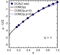
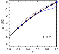
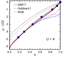
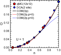
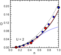
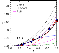
Figure 1: (Colour online) Scaled chemical potential $\mu-{U}/{2}$ (top row) and double occupancy $D$ (bottom row) as functions of the filling $n$ for $U=1$ (left-hand column), $2$ (central column) and $4$ (right-hand column) and $T={1}/{6}$ for COM(3p) (black lines), COM(2p,$p>0$) (dashed red line) and COM(2p,$p<0$) (dotted blue line). COM results are compared with $12\times 12$-site qMC [94] and $2$-site DCA [95] numerical data (red and blue circles, respectively) as well as with the results of Hubbard I (dot-dashed green line) and Roth (dot-dot-dashed magenta line) methods (only at $U=4$). The thin black dashed and dotted lines in central and right-hand columns are COM(3p) results for $U=1$ and $U=2$, respectively. From [46] with kind permission of The European Physical Journal (EPJ).

In figure 1, we report the behaviour of the chemical potential $\mu$ and of the double occupancy $D$ as functions of the filling $n$ for $U=1$, $2$ and $4$ and $T={1}/{6}$. The COM $3$-pole solution [COM(3p)] is clearly in very good agreement for all values of $U$ reported in the whole range of filling $n$ with the $12\times 12$-site qMC [94] and $2$-site DCA [95] numerical data. COM(3p) also catches the change of concavity in the chemical potential in proximity of half filling between $U=1,2$ and $U=4$ [figure 1 (top row)] reported by the DCA data. Also the COM $2$-pole solution with the $p$ parameter positive [COM(2p, $p>0$)] manages, but not COM(2p, $p<0$), Hubbard I and Roth solutions, which always present the same concavity. $U=4$ already drives quite strong electronic correlations, and the chemical potential shows a tendency towards a gap opening at $n=1$. The double occupancy $D$ [figure 1 (bottom row)] reports a clear change of correlation-strength regime between $U=1,2$ and $U=4$: it goes from a parabolic-like behaviour resembling the non-interacting one (${n^{2}}/{4}$) at $U=1,2$ [figure 1 (bottom-left/central panels)] to a behaviour presenting a change of slope on approaching half filling at $U=4$ [figure 1 (bottom-right panel)]. COM(3p) only describes correctly these features. COM(3p) evidently has [see figure 1 (bottom-central/right panels)] the capability to correctly interpolate between the two COM(2p) solutions sticking to COM(2p, $p<0$) at low-intermediate values of filling and even improving on COM(2p, $p>0$) at larger values of filling.

4 Residual self-energy and cuprate superconductors

4.1 Theory

In this case, we choose as basic field just the composite doublet field operator $\psi\left(i\right)=\left(\xi^{\dagger}\left(i\right),\eta^{\dagger}\left(i\right)\right)$. By considering the two-time thermodynamic GF [96, 97, 98], we define the retarded GF $G(i,j)=\langle R[\psi(i)\psi^{\dagger}(j)]\rangle$ $=\theta(t_{i}-t_{j})\langle\{\psi(i),\,\psi^{\dagger}(j)\}\rangle$ that satisfies the following equation

$$\Lambda(\partial_{i})G(i,j)\Lambda^{\dagger}(\overleftarrow{\partial}_{j})=\Lambda(\partial_{i})G_{0}(i,j)\Lambda^{\dagger}(\overleftarrow{\partial}_{j})+\langle R[\delta J(i)\delta J^{\dagger}(j)]\rangle\,,$$ (4.1)

where the derivative operator $\Lambda(\partial_{i})=\mathrm{i}\frac{\partial}{\partial t_{i}}-\varepsilon(-\mathrm{i}\nabla_{i})$ and the propagator $G^{0}(i,j)$ is defined by the equation $\Lambda(\partial_{i})G^{0}(i,j)=\mathrm{i}\delta(t_{i}-t_{j})I(i,j)$. By introducing the Fourier transform, equation (4.1) can be formally solved as

$$G(\mathbf{k},\omega)=\frac{1}{\omega-\varepsilon(\mathbf{k})-\Sigma(\mathbf{k},\omega)}I(\mathbf{k})\,,$$ (4.2)

where the self-energy $\Sigma(\mathbf{k},\omega)$ has the expression $\Sigma(\mathbf{k},\omega)=B_{irr}(\mathbf{k},\omega)I^{-1}(\mathbf{k})$ with $B(\mathbf{k},\omega)=$ $\mathcal{F}\langle R[\delta J(i)\delta J^{\dagger}(j)]\rangle$. Equation (4.2) is the Dyson equation for composite fields and represents the starting point for a perturbative calculation in terms of the propagator $G^{0}(\mathbf{k},\omega)=\frac{1}{\omega-\varepsilon(\mathbf{k})}I(\mathbf{k})$, which corresponds to the $2$-pole approximation and can be easily obtained by the calculations in the previous sections.

The calculation of the self-energy $\Sigma(\mathbf{k},\omega)$ requires the calculation of the higher-order propagator $B(\mathbf{k},\omega)$. We shall compute this quantity by using the non-crossing approximation (NCA). By neglecting the pair term $c(i)c^{\dagger\alpha}(i)c(i)$, the source $J(i)$ can be written as $J(\mathbf{i},t)=\sum_{\mathbf{j}}a(\mathbf{i,j},t)\psi(\mathbf{j},t)$ where

$$a_{11}(\mathbf{i,j},t)=-\mu\delta_{\mathbf{ij}}-4t\alpha_{\mathbf{ij}}-2t\sigma^{\mu}n_{\mu}(i)\alpha_{\mathbf{ij}}\,,\quad a_{12}(\mathbf{i,j},t)=-4t\alpha_{\mathbf{ij}}-2t\sigma^{\mu}n_{\mu}(i)\alpha_{\mathbf{ij}}\,,$$

$$a_{21}(\mathbf{i,j},t)=2t\sigma^{\mu}n_{\mu}(i)\alpha_{\mathbf{ij}}\,,\quad a_{22}(\mathbf{i,j},t)=(U-\mu)\delta_{\mathbf{ij}}+2t\sigma^{\mu}n_{\mu}(i)\alpha_{\mathbf{ij}}.$$ (4.3)

Then, for the calculation of $B_{irr}(i,j)=\langle R[\delta J(i)\delta J^{\dagger}(j)]\rangle_{irr}$, we approximate $\delta J(\mathbf{i},t)\approx\sum_{\mathbf{j}}[a(\mathbf{i,j},t)-$ $\langle a(\mathbf{i,j},t)\rangle]\psi(\mathbf{j},t)$ and, therefore, $B_{irr}(i,j)=4t^{2}F(i,j)(1-\sigma_{1})$ where we defined $F(i,j)=$ $\langle R[\sigma^{\mu}\delta n_{\mu}(i)c^{\alpha}(i)c^{\dagger\alpha}(j)\delta n_{\lambda}(j)\sigma^{\lambda}]\rangle$ with $\delta n_{\mu}(i)=n_{\mu}(i)-\langle n_{\mu}(i)\rangle$. The self-energy is then written as

$$\Sigma(\mathbf{k},\omega)=4t^{2}F(\mathbf{k},\omega)\left(\begin{array}[]{cc}I_{11}^{-2}&-I_{11}^{-1}I_{22}^{-1}\vspace{1mm}\\ -I_{11}^{-1}I_{22}^{-1}&I_{22}^{-2}\end{array}\right).$$ (4.4)

In order to calculate the retarded function $F(i,j)$, first we use the spectral theorem to express

$$F(i,j)=\frac{\mathrm{i}}{2\piup}\int_{-\infty}^{+\infty}\mathrm{d}\omega\mathrm{e}^{-\mathrm{i}\omega(t_{i}-t_{j})}\frac{1}{2\piup}\int_{-\infty}^{+\infty}\mathrm{d}\omega^{\prime}\frac{1+\mathrm{e}^{-\beta\omega^{\prime}}}{\omega-\omega^{\prime}+\mathrm{i}\varepsilon}C(\mathbf{i-j},\omega^{\prime})\,,$$ (4.5)

where $C(\mathbf{i-j},\omega^{\prime})$ is the correlation function $C(i,j)=\langle\sigma^{\mu}\delta n_{\mu}(i)c^{\alpha}(i)c^{\dagger\alpha}(j)\delta n_{\lambda}(j)\sigma^{\lambda}\rangle$. Next, we use the NCA and approximate $\langle\sigma^{\mu}\delta n_{\mu}(i)c^{\alpha}(i)c^{\dagger\alpha}(j)\delta n_{\lambda}(j)\sigma^{\lambda}\rangle\approx\langle\delta n_{\mu}(i)\delta n_{\mu}(j)\rangle\langle c^{\alpha}(i)c^{\dagger\alpha}(j)\rangle$. By means of this decoupling and using again the spectral theorem, we finally have

$$F(\mathbf{k},\omega) = \frac{1}{\piup}\int_{-\infty}^{+\infty}\mathrm{d}\omega^{\prime}\frac{1}{\omega-\omega^{\prime}+\mathrm{i}\delta}\frac{a^{2}}{(2\piup)^{3}}\int\mathrm{d}^{2}p\mathrm{d}\Omega\alpha^{2}(p)$$ (4.6)

$$\times \left[\tanh\frac{\beta\Omega}{2}+\coth\frac{\beta(\omega^{\prime}-\Omega)}{2}\right]\mathop{\symoperators Im}\nolimits[G_{cc}(\mathbf{p},\Omega)]\mathop{\symoperators Im}\nolimits[\chi(\mathbf{k-p},\omega^{\prime}-\Omega)]\,,$$

where $G_{cc}(\mathbf{k},\omega)=\sum_{a,b=1}^{2}G_{ab}(\mathbf{k},\omega)$ is the retarded electronic GF and $\chi(\mathbf{k},\omega)=\sum_{\mu}\mathcal{F}\langle R[\delta n_{\mu}(i)\delta n_{\mu}(j)]\rangle$ is the total charge and spin dynamical susceptibility. The result (4.6) shows that the self-energy calculation requires the knowledge of the bosonic propagator. Remarkably, up to this point, the system of equations for the GF and the anomalous self-energy is similar to the one derived in the two-particle self-consistent approach (TPSC) [99, 100], the DMFT$+\Sigma$ approach [101, 102, 103, 104, 105] and a Mori-like approach by Plakida and coworkers [41, 42, 43]. It would be the way to compute the dynamical spin and charge susceptibilities to be completely different because, instead of relying on a phenomenological model and neglecting the charge susceptibility like these approaches do, we will use a self-consistent two-pole approximation [51].

Finally, the electronic GF $G(\mathbf{k},\omega)$ is computed through the following self-consistency scheme: we first compute $G^{0}(\mathbf{k},\omega)$ and $\chi_{\mu}(\mathbf{k},\omega)$ in the two-pole approximation, then $\Sigma(\mathbf{k},\omega)$ and consequently $G(\mathbf{k},\omega)$. Finally, we check how much the fermionic parameters ($\mu$, $\Delta$, and $p$) changed and decide whether to stop or to continue by computing new $\chi_{{}_{\mu}}(\mathbf{k},\omega)$ and $\Sigma(\mathbf{k},\omega)$ after $G(\mathbf{k},\omega)$.

4.2 Results

We intend to characterize some electronic properties by computing the spectral function $A(\mathbf{k},\omega)=-\frac{1}{\piup}\mathop{\symoperators Im}\nolimits[G_{cc}(\mathbf{k},\omega)]$ and the density of states per spin $N(\omega)=\frac{1}{(2\piup)^{2}}\int\mathrm{d}^{2}kA(\mathbf{k},\omega)$. We also investigate the electronic self-energy $\Sigma_{cc}(\mathbf{k},\omega)$, defined through the equation

$$G_{cc}(\mathbf{k},\omega)=\frac{1}{\omega-\epsilon_{0}(\mathbf{k})-\Sigma_{cc}(\mathbf{k},\omega)}\,,$$ (4.7)

where $\epsilon_{0}(\mathbf{k})=-\mu-4t\alpha(\mathbf{k})$ is the non-interacting dispersion, and introduce the quantity $r(\mathbf{k})=\epsilon_{0}(\mathbf{k})+\Sigma^{\prime}_{cc}(\mathbf{k},\omega=0)$ that determines the Fermi surface locus in the momentum space, $r(\mathbf{k})=0$, in a Fermi liquid. The actual Fermi surface (or its relic in a non-Fermi-liquid) is given by the relative maxima of $A(\mathbf{k},\omega=0)$, which takes into account, on equal footing, both $\Sigma^{\prime}_{cc}(\mathbf{k},\omega)$ and $\Sigma^{\prime\prime}_{cc}(\mathbf{k},\omega)$, and is directly related, within the sudden approximation and forgetting any selection rules, to the effective ARPES measurements.

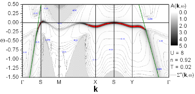
Figure 2: (Colour online) Spectral function $A(\mathbf{k},\omega)$ close to the chemical potential ($\omega=0$) along the principal directions [$\Gamma=(0,\,0)\to S=(\piup/2,\,\piup/2)\to M=(\piup,\,\piup)$, $M\to X=(\piup,\,0)$, $X\to Y=(0,\,\piup)$ and $Y\to\Gamma$] for $U=8$, ${T=0.02}$ and $n=0.92$. From [15].

4.2.1 Spectral function and dispersion

The electronic dispersion, or better its relic in a strongly correlated system, can be obtained through the relative maxima of $A(\mathbf{k},\omega)$. In figure 2, we show the latter, in scale of grays (red is for the above-scale values), along the principal directions [$\Gamma=(0,\,0)\to S=(\piup/2,\,\piup/2)\to M=(\piup,\,\piup)$, $M\to X=(\piup,\,0)$, $X\to Y=(0,\,\piup)$ and $Y\to\Gamma$] for $U=8$, $T=0.02$ and $n=0.92$. The light gray lines and uniform areas are labeled with the values of $\Sigma^{\prime\prime}(\mathbf{k},\omega)$. The dark green lines are guides to the eye, signaling the direction of the dispersion just before the visible kink separating the black and the red areas of the dispersion. The latter is well-defined (red areas) only in the regions where $\Sigma^{\prime\prime}(\mathbf{k},\omega)$ is zero or almost negligible. In the regions where $\Sigma^{\prime\prime}(\mathbf{k},\omega)$ is instead finite, $A(\mathbf{k},\omega)$ assumes very low values, very difficult to be detected by ARPES, which, accordingly, would report only the red areas in the picture. This is crucial to understand the experimental evidences on the Fermi surface in the underdoped regime and to explain ARPES findings together with those of quantum oscillations measurements.

The dispersion loses significance close to $M$ where $A(\mathbf{k},\omega)$ loses weight as $\Sigma^{\prime\prime}(\mathbf{k},\omega)$ increases: correspondingly, $\chi_{3}\left(\mathbf{k},\omega\right)$ is strongly peaked at $M$ due to the strong antiferromagnetic correlations in the system. The bandwidth reduces from $4t$ to values of the order $J={4t^{2}}/{U}=0.5t$, as expected for the dispersion of few holes in a strong antiferromagnetic background. The characteristics of the dispersion are also compatible with this scenario, such as the sequence of minima and maxima, actually driven by the doubling of the Brillouin zone induced by the strong antiferromagnetic correlations, as well as the dynamical formation of a $t^{\prime}$ diagonal hopping indicated by the pronounced warping of the dispersion along the $X\to Y$ direction. Moreover, remarkably, the dispersion at $X$($Y$) coming from both $\Gamma$ and $M$ is substantially flat: this feature is in very good agreement both with qMC computations (see [106] and references therein) and with ARPES experiments [107], which detect a similar behaviour for overdoped systems. It is worth noting that such flatness at $X$($Y$) is present for larger dopings too ($n=0.7,$ $0.78$ and $0.85$), as shown in figure 3 of reference [15], and that the extension of the plateau increases upon decreasing the doping. It is now clear that the dispersion warping along $X\to Y$, displayed in figure 2, is also responsible for two maxima in $N\left(\omega\right)$: one related to the van-Hove singularities at $X$ and $Y$ and one to the dispersion maximum close to $S$. The entity of the dip between these two maxima just depends on the number of available well-defined (red) states in $\mathbf{k}$ present between these two values of $\omega$. This will determine the formation of a more or less pronounced pseudogap in $N\left(\omega\right)$, as we will discuss after the analysis of the region close to $M$.

Definitely, the absence of spectral weight close to $M$ and, in particular and surprisingly, at $\omega=0$ (i.e., on the Fermi surface, in contradiction with the Fermi-liquid scenario), is the most relevant result of this study: it will determine almost all relevant and anomalous features of the single-particle properties. Last, but not least, quite remarkable is also the presence of kinks in the dispersion in both the nodal ($\Gamma\to M$) and the antinodal ($X\to\Gamma$) directions, as highlighted by the dark green guidelines, in qualitative agreement with some ARPES experiments [108]. Remarkably, similar results for the single-particle excitation spectrum were obtained in the self-consistent projection operator method [109, 110], the operator projection method [111, 112, 113] and a Mori-like approach by Plakida and coworkers [42, 43].

4.2.2 Spectral function and Fermi surface

Considering $A(\mathbf{k},\omega=0)$, we attain the closest concept to Fermi surface for a strongly correlated system. In figure 3, we show $A(\mathbf{k},\omega=0)$ as a function of $\mathbf{k}$ in a quarter of the Brillouin zone for $U=8$ and (left) $n=0.85$ and $T=0.01$ and (right) $n=0.92$ and $T=0.02$. According to the interpretation of the ARPES measurements in the sudden approximation [107, 108], the Fermi surface can be defined as the locus in $\mathbf{k}$ space of the relative maxima of $A(\mathbf{k},\omega=0)$. Such a definition leads to a possible explanation of ARPES measurements, but also allows one to go beyond them, with their finite resolution and sensitivity, aiming at a reconciliation with other types of measurements, in particular quantum oscillations ones, which seemingly report results in disagreement, also up to dichotomy in some cases, with ARPES.

The evolution of the Fermi surface topology on increasing $n$ is the consequence of two Lifshitz transitions [114], at $n\cong 0.82$ and $n\cong 0.9$. The first Lifshitz transition ($n\cong 0.82$, not shown) is due to the crossing of the chemical potential by the van Hove singularity: the exact doping can be easily identified by looking at the chemical potential behaviour as a function of $n$ (not shown). The second transition ($n\cong 0.9$, not shown) is characterized by the formation of a hole pocket in the proximity of $S$. Changes in the Fermi-surface topology were also found in other studies on the cuprates [115, 37, 42]. A very detailed analysis for the Lifshitz transitions in the $t$-$J$ model was performed by Korshunov and Ovchinnikov [116]: they obtained the model parameters from ab initio calculations for cuprates [117] and found a large overdoped Fermi surface for $n<0.76$, two concentric Fermi surfaces for $0.76<n<0.85$ and a small hole Fermi surface around $S$ for $n>0.85$. Consequently, in reference [118], Ovchinnikov et al. characterized better these two quantum phase transitions, obtaining a logarithmic singularity for $N\left(\omega=0\right)$ at $n=0.85$ and a stepwise feature at $n=0.76$.

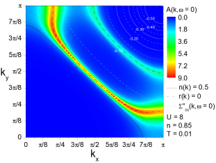
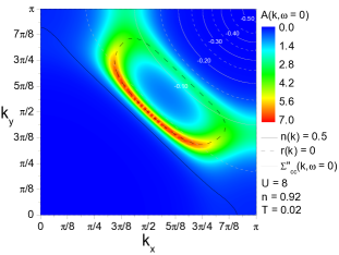
Figure 3: (Colour online) Spectral function at the chemical potential $A(\mathbf{k},\omega=0)$ as a function of momentum $\mathbf{k}$ for $U=8$, $T=0.01$ and (left) $n=0.85$ and (right) $n=0.92$ ($T=0.02$). The solid line marks the locus $n(\mathbf{k})=0.5$, the dashed line marks the locus $r(\mathbf{k})=0$, the gray lines are labeled with the values of $\Sigma^{\prime\prime}_{cc}(\mathbf{k},\omega=0)$, and the dotted line is a guide to the eye and marks the reduced (antiferromagnetic) Brillouin zone. From [15].

Then, in figure 3, we report results for $n=0.85$ and $n=0.92$ as representatives of two non-trivial topologies of the Fermi surface. We can clearly distinguish two arcs that for $n=0.92$ somehow join. Given the current sensitivities, only the arc with the larger intensities, among the two, may be visible to ARPES: at $n=0.92$, the region close to $S$ is the only one with an appreciable signal. The less-intense arc, reported in reference [42] too, is the relic of a shadow band, as clearly seen in figure 2, and thus never changes its curvature, in contrast to what happens to the other arc, subject to the crossing of the van Hove singularity ($n\cong 0.82$, not shown).

Three additional ingredients can help us better understand the evolution with doping of the Fermi surface: (i) the $n(\mathbf{k})=0.5$ locus (solid line), i.e., the Fermi surface if the system would be non-interacting; (ii) the $r(\mathbf{k})=0$ locus (dashed line), i.e., the Fermi surface if the system would be a Fermi liquid or a state close to it conceptually; (iii) the values (grey lines and labels) of $\Sigma^{\prime\prime}_{cc}(\mathbf{k},\omega=0)$. Through the combined analysis of these three ingredients with the positions and intensities of the relative maxima of $A(\mathbf{k},\omega=0)$, we can understand better what these latter imply and classify the behaviour of the system on changing filling. At high dopings (not shown), the positions of the two arcs match exactly $r(\mathbf{k})=0$ lines: this fact corroborates our definition of Fermi surface, making it versatile and valid beyond the Fermi liquid picture without contradicting this latter. Increasing the filling, we find the first topological transition from a Fermi surface closed around $\Gamma$ (hole like in cuprates language) to a Fermi surface closed around $M$ (electron like in cuprates language) at $n\cong 0.82$ (not shown), where the van Hove singularity is at $\omega=0$ [see figure 3 (left-hand panel) for $n=0.85$, a close doping]. Close to the antinodal points ($X$ and $Y$), a net discrepancy between the position of the relative maxima of $A(\mathbf{k},\omega=0)$ and the line $n(\mathbf{k})=0.5$ arises on decreasing doping. This feature does not only allow the topological transition, absent for the $n(\mathbf{k})=0.5$ locus that reaches the anti-diagonal ($X\to Y$) at $n=1$ satisfying the Luttinger theorem, but it also accounts for the broadening of the relative maxima of $A(\mathbf{k},\omega=0)$ close to the anti-nodal points. The broadening is due to the small, but finite, value of $\Sigma^{\prime\prime}_{cc}(\mathbf{k},\omega=0)$ in those regions, signaling the net enhancement of the correlation strength, and then the impossibility to consider the system in this regime as a conventional non- (or weakly-) interacting one within a Fermi-liquid scenario or its ordinary extensions for ordered phases. The emergence of such features only in well defined regions in $\mathbf{k}$ space is of great interest and goes beyond the problem under analysis (cuprates).

As the most important result, at $n=0.92$, the relative maxima of $A(\mathbf{k},\omega=0)$ deviate also from the $r(\mathbf{k})=0$ line, at least partially, leading to a completely new scenario: $r(\mathbf{k})=0$ defines a pocket, while the peaks of $A(\mathbf{k},\omega=0)$ feature the very same pocket together with quite well-defined wings closing, with one half of the pocket, a kind of relic of a large Fermi surface. This is the second and most surprising topological transition for the Fermi surface; in fact, the two arcs, clearly visible for all other dopings, join and do not close just a pocket, as expected from the conventional theory for an antiferromagnet: they develop a fully independent branch. The actual Fermi surface is neither a pocket nor a large Fermi surface. This very unexpected result can be connected to the dichotomy between the experiments (e.g., ARPES) pointing to a small and the ones (e.g., quantum oscillations) pointing to a large Fermi surface.

The pocket too is definitely unconventional. In fact, there are two distinct halves of the pocket: one with very high intensity pinned at $S$ (the only possibly detectable by ARPES) and one with very low intensity (detectable only by some quantum oscillations experiments). This is our interpretation for the Fermi arcs, seen in many ARPES experiments [108, 119] and unaccountable for any ordinary theory based on the Fermi liquid picture, though modified by including an incipient spin or charge ordering. Clearly, looking only at the Fermi arc (as necessarily in ARPES), the Fermi surface looks ill defined, not enclosing a definite region of $\mathbf{k}$ space, but having access also to the other half of the pocket, such problem is greatly alleviated. In our understanding, the antiferromagnetic fluctuations are so strong to destroy the quasi-particle coherence in that region of $\mathbf{k}$ space, as similarly reported in the DMFT$+\Sigma$ approach [101, 102, 103, 104, 105] and in a Mori-like approach by Plakida and collaborators [42, 43]. The Fermi arc is pinned at $S$: this pinning of the center of mass of the ARPES-visible Fermi arc has been obtained also in ARPES experiments [120].

4.2.3 Density of states and pseudogap

The other main feature in underdoped cuprates is a substantial depletion in the electronic $N\left(\omega\right)$: the pseudogap. In figure 4 (left-hand panel), we show $N(\omega)$ for $U=8$ and four couples of values of filling and temperature: $n=0.7$ and $T=0.01$, $n=0.78$ and $T=0.01$, $n=0.85$ and $T=0.01$, and $n=0.92$ and $T=0.02$, in the frequency region close to the chemical potential. As a reference, we also show, in figure 4 (right-hand panel), $A(\mathbf{\underline{k}},\omega\sim 0)$ at $\mathbf{\underline{k}}=S=(\piup/2,\piup/2)$, $\mathbf{\underline{k}}=\underline{S}$ which is where the phantom half of the pocket touches the diagonal $\Gamma\to M$ (i.e., where the dispersion cuts the diagonal $\Gamma\to M$ closer to $M$), and $\mathbf{\underline{k}}=X$ for $U=8$, $n=0.92$ and $T=0.02$. As apparent in figure 4 (left-hand panel), $N\left(\omega\right)$ has two maxima separated by a dip, which plays the role of pseudogap. Its presence is due to the dispersion warping along the $X\to Y$ direction (see figure 2), which induces the two maxima [one due to the van-Hove singularity at $X$ and one due to the dispersion maximum close to $S$ — see figure 4 (right-hand panel)] and the loss of states, in this frequency window, in the region in $\mathbf{k}$ close to $M$. In order to realize the weight loss due to the finite value of $\Sigma^{\prime\prime}_{cc}(\mathbf{k},\omega=0)$ in the region in $\mathbf{k}$ close to $M$, we can look at the impressive difference between the values of $A(\underline{S},\omega=0)$ and $A(S,\omega=0)$ [figure 4 (right-hand panel)]. Increasing the filling, there is a net spectral weight transfer between the two maxima; in particular, from the dispersion top close to $S$ to the antinodal point $X$, where the van Hove singularity resides. At the lowest doping ($n=0.92$), a well formed pseudogap can be seen for $\omega<0$ and will clearly influence the properties of the system. For $n=0.92$, we do not find any divergence of $\Sigma^{\prime}_{cc}(\mathbf{k},\omega=0)$, in contrast to what is stated in reference [121] where this feature is presented as the definite reason for the pseudogap formation. In our study, the pseudogap is just the result of the weight transfer from the single-particle density of states to the two-particle one, related to the (antiferro)magnetic excitations occurring in the system on decreasing doping at low $T$. A similar doping behaviour of the pseudogap has been found by the DMFT$+\Sigma$ approach [101, 102, 103, 104, 105], a Mori-like approach by Plakida and collaborators [42, 43] and the cluster perturbation theory [122, 123, 100].

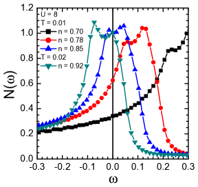
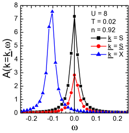
Figure 4: (Colour online) (left) Density of states $N(\omega)$ as a function of frequency $\omega$ for $U=8$, (black squares) $n=0.7$ and $T=0.01$, (red circles) $n=0.78$ and $T=0.01$, (blue up triangles) $n=0.85$ and $T=0.01$, and (green down triangles) $n=0.92$ and $T=0.02$. (right) Spectral function in proximity of the chemical potential $A(\mathbf{\underline{k}},\omega\sim 0)$ at (black squares) $\mathbf{\underline{k}}=S=(\piup/2,\piup/2)$, (red circles) $\underline{S}$ (in the text), and (blue triangles) $X=(\piup,\,0)$ for $U=8$, $n=0.92$ and $T=0.02$. From [15].

5 Conclusions

In this review paper, written in honor of the $80^{\textrm{th}}$ anniversary of Professor Ihor Stasyuk, we have illustrated the composite operator method by means of a prototypical example: the 2D Hubbard model and its application to the description of high-$T_{\text{c}}$ cuprate superconductors. The method has been reported first for a general case in order to appreciate its philosophy and its capability to be applied to any strongly correlated system in a controlled fashion.

Ukrainian 0

Ïiäõiä ìåòîäó êîìïîçèòíèõ îïåðàòîðiâ äî äâîâèìiðíî¿ ìîäåëi Õàááàðäà òà êóïðàòiâ À. Äi Чüîëî${}^{\textsf{\footnotesize{\mbox{?}}}}$, À. Àâåëëà${}^{\textsf{\footnotesize{\mbox{?},\penalty 1000\mbox{?},\penalty 1000\mbox{?}}}}$

             
${}^{\textsf{\footnotesize 1}}$ ôàêóëüòåò ôiçèêè ‘‘Å.Ð. Caianiello’’, óíiâåðñèòåò Ñàëåðíî, I-84084 Ôiøiàíî (Ñàëåðíî), Iòàëiÿ ${}^{\textsf{\footnotesize 2}}$ CNR-SPIN, óíiâåðñèòåò Ñàëåðíî, I-84084 Ôiøiàíî (Ñàëåðíî), Iòàëiÿ ${}^{\textsf{\footnotesize 3}}$ âiääiëåííÿ CNISM â Ñàëåðíî, óíiâåðñèòåò Ñàëåðíî, I-84084 Ôiøiàíî (Ñàëåðíî), Iòàëiÿ

References

- [1] Anderson P.W., Science, 1972, 177, 393, doi:10.1126/science.177.4047.393.
-
[2]
Georges A., Kotliar G., Krauth W., Rozenberg M.J., Rev. Mod. Phys., 1996,
68, 13,
doi:10.1103/RevModPhys.68.13. - [3] Hewson A.C., The Kondo Problem to Heavy Fermions, Cambridge University Press, Cambridge, 1997.
- [4] Avella A., Mancini F. (Eds.), Strongly Correlated Systems: Theoretical Methods, Springer Series in Solid-State Sciences, Vol. 171, Springer, Berlin–Heidelberg, 2012.
- [5] Avella A., Mancini F. (Eds.), Strongly Correlated Systems: Numerical Methods, Springer Series in Solid-State Sciences, Vol. 176, Springer, Berlin–Heidelberg, 2013.
- [6] Avella A., Mancini F. (Eds.), Strongly Correlated Systems: Experimental Techniques, Springer Series in Solid-State Sciences, Vol. 180, Springer, Berlin–Heidelberg, 2015.
- [7] Bednorz J.G., Müller K.A., Z. Phys. B, 1986, 64, 189, doi:10.1007/BF01303701.
- [8] Wu M.K., Ashburn J.R., Torng C.J., Hor P.H., Meng R.L., Gao L., Huang Z.J., Wang Y.Q., Chu C.W., Phys. Rev. Lett., 1987, 58, 908, doi:10.1103/PhysRevLett.58.908.
- [9] Timusk T., Statt B., Rep. Prog. Phys., 1999, 62, 61, doi:10.1088/0034-4885/62/1/002.
- [10] Norman M.R., Pines D., Kallin C., Adv. Phys., 2005, 54, 715, doi:10.1080/00018730500459906.
- [11] Lee P.A., Nagaosa N., Wen X.-G., Rev. Mod. Phys., 2006, 78, No. 1, 17, doi:10.1103/RevModPhys.78.17.
- [12] Armitage N.P., Fournier P., Greene R.L., Rev. Mod. Phys., 2010, 82, 2421, doi:10.1103/RevModPhys.82.2421.
- [13] Fradkin E., Kivelson S.A., Nat. Phys., 2012, 8, 864, doi:10.1038/nphys2498.
-
[14]
Rice T.M., Yang K.-Y., Zhang F.C., Rep. Prog. Phys.,
2012, 75, No. 1, 016502,
doi:10.1088/0034-4885/75/1/016502. - [15] Avella A., Adv. Condens. Matter Phys., 2014, 2014, 515698, doi:10.1155/2014/515698.
-
[16]
Keimer B., Kivelson S.A., Norman M.R., Uchida S., Zaanen J., Nature, 2015,
518, 179,
doi:10.1038/nature14165. - [17] Avella A., Buonavolontà C., Guarino A., Valentino M., Leo A., Grimaldi G., de Lisio C., Nigro A., Pepe G., Phys. Rev. B, 2016, 94, 115426, doi:10.1103/PhysRevB.94.115426.
- [18] Novelli F., Giovannetti G., Avella A., Cilento F., Patthey L., Radovic M., Capone M., Parmigiani F., Fausti D., Phys. Rev. B, 2017, 95, 174524, doi:10.1103/PhysRevB.95.174524.
- [19] Avella A., Physica B, 2018, 536, 713–716, doi:10.1016/j.physb.2017.11.031.
- [20] Anderson P.W., Science, 1987, 235, 1196, doi:10.1126/science.235.4793.1196.
- [21] J. Hubbard, Proc. R. Soc. London, Ser. A, 1963, 276, 238, doi:10.1098/rspa.1963.0204.
- [22] J. Hubbard, Proc. R. Soc. London, Ser. A, 1964, 277, 237, doi:10.1098/rspa.1964.0019.
- [23] J. Hubbard, Proc. R. Soc. London, Ser. A, 1964, 281, 401, doi:10.1098/rspa.1964.0190.
- [24] Emery V.J., Phys. Rev. Lett., 1987, 58, 2794, doi:10.1103/PhysRevLett.58.2794.
- [25] Emery V.J., Reiter G., Phys. Rev. B, 1988, 38, 4547, doi:10.1103/PhysRevB.38.4547.
- [26] Emery V.J., Kivelson S.A., Physica C, 1994, 235, 189, doi:10.1016/0921-4534(94)91345-5.
- [27] Oleś A.M., Spałek J., Z. Phys. B, 1981, 44, 177, doi:10.1007/BF01297173.
- [28] Zhang F.C., Rice T.M., Phys. Rev. B, 1988, 37, 3759, doi:10.1103/PhysRevB.37.3759.
- [29] Abanov Ar., Chubukov A.V., Schmalian J., Adv. Phys., 2003, 52, 119, doi:10.1080/0001873021000057123.
- [30] Kuz’min E.V., Ovchinnikov S.G., Teor. Mat. Fiz., 1977, 31, 379–391 (in Russian), [Theor. Math. Phys., 1977, 31, 523–531, doi:10.1007/BF01030571].
-
[31]
Tserkovnikov Y.A., Teor. Mat. Fiz., 1981, 49, 219–233 (in Russian), [Theor. Math. Phys., 1981, 49, 993–1002,
doi:10.1007/BF01028994]. -
[32]
Tserkovnikov Y.A., Teor. Mat. Fiz., 1982, 50, 261–271 (in Russian), [Theor. Math. Phys., 1982, 50, 171–177,
doi:10.1007/BF01015298]. - [33] Mori H., Prog. Theor. Phys., 1965, 33, 423, doi:10.1143/PTP.33.423.
- [34] Rowe D.J., Rev. Mod. Phys., 1968, 40, 153, doi:10.1103/RevModPhys.40.153.
- [35] Roth L.M., Phys. Rev., 1969, 184, 451, doi:10.1103/PhysRev.184.451.
- [36] Nolting W., Borgieł W., Phys. Rev. B, 1989, 39, 6962, doi:10.1103/PhysRevB.39.6962.
- [37] Barabanov A.F., Kovalev A.A., Urazaev O.V., Belemuk A.M., Hayn R., J. Exp. Theor. Phys., 2001, 92, No. 4, 677–695, doi:10.1134/1.1371349.
- [38] Val’kov V.V., Dzebisashvili D.M., J. Exp. Theor. Phys., 2005, 100, No. 3, 608–616, doi:10.1134/1.1901772.
- [39] Plakida N.M., Oudovenko V.S., Phys. Rev. B, 1999, 59, 11949–11961, doi:10.1103/PhysRevB.59.11949.
- [40] Plakida N.M., JETP Lett., 2001, 74, No. 1, 36–40, doi:10.1134/1.1402203.
- [41] Plakida N.M., Anton L., Adam S., Adam Gh., J. Exp. Theor. Phys., 2003, 97, 331, doi:10.1134/1.1608998.
- [42] Plakida N.M., Oudovenko V.S., J. Exp. Theor. Phys., 2007, 104, 230, doi:10.1134/S1063776107020082.
- [43] Plakida N., High-Temperature Cuprate Superconductors, Springer Series in Solid-State Sciences, Vol. 166, Springer, Berlin–Heidelberg, 2010.
- [44] Ovchinnikov S.G., Nikolaev S.V., JETP Lett., 2011, 93, No. 9, 517–520, doi:10.1134/S0021364011090116.
- [45] Mancini F., Avella A., Adv. Phys., 2004, 53, No. 5–6, 537, doi:10.1080/00018730412331303722.
- [46] Avella A., Eur. Phys. J. B, 2014, 87, 45, doi:10.1140/epjb/e2014-40630-7.
-
[47]
Avella A., Mancini F., Villani D., Siurakshina L., Yushankhai V.,
Int. J. Mod. Phys. B, 1998, 12, No. 1, 81,
doi:10.1142/S0217979298000065. -
[48]
Avella A., Mancini F., Villani D., Matsumoto H., Physica C, 1997, 282, 1757,
doi:10.1016/S0921-4534(97)00944-1. - [49] Avella A., Mancini F., Münzner R., Phys. Rev. B, 2001, 63, 245117, doi:10.1103/PhysRevB.63.245117.
-
[50]
Avella A., Mancini F., Sánchez-López M.d.M.,
Eur. Phys. J. B, 2002, 29, 399,
doi:10.1140/epjb/e2002-00323-6. - [51] Avella A., Mancini F., Turkowski V., Phys. Rev. B, 2003, 67, 115123, doi:10.1103/PhysRevB.67.115123.
- [52] Avella A., Mancini F., Saikawa T., Eur. Phys. J. B, 2003, 36, 445, doi:10.1140/epjb/e2004-00002-8.
- [53] Avella A., Mancini F., Plekhanov E., Physica C, 2010, 470, S930, doi:10.1016/j.physc.2010.02.087.
-
[54]
Avella A., Mancini F., Mancini F.P., Plekhanov E., J. Phys. Chem. Solids, 2011, 72, 362,
doi:10.1016/j.jpcs.2010.10.015. - [55] Odashima S., Avella A., Mancini F., Phys. Rev. B, 2005, 72, No. 20, 205121, doi:10.1103/PhysRevB.72.205121.
- [56] Avella A., Mancini F., Villani D., Phys. Lett. A, 1998, 240, 235, doi:10.1016/S0375-9601(98)00030-9.
- [57] Avella A., Mancini F., Villani D., Matsumoto H., Eur. Phys. J. B, 2001, 20, 303, doi:10.1007/PL00011101.
- [58] Avella A., Mancini F., Physica C, 2004, 408, 284, doi:10.1016/j.physc.2004.02.147.
-
[59]
Avella A., Mancini F., Mancini F.P., Plekhanov E., J. Phys. Chem. Solids, 2011,
72, 384,
doi:10.1016/j.jpcs.2010.10.030. -
[60]
Avella A., Mancini F., Mancini F.P., Plekhanov E., J. Phys. Conf. Ser., 2011, 273, 012091,
doi:10.1088/1742-6596/273/1/012091. -
[61]
Avella A., Mancini F., Mancini F.P., Plekhanov E., J. Phys. Conf. Ser., 2012,
391, 012121,
doi:10.1088/1742-6596/391/1/012121. -
[62]
Avella A., Mancini F., Mancini F.P., Plekhanov E., Eur. Phys. J. B, 2013, 86, 265,
doi:10.1140/epjb/e2013-40115-3. - [63] Avella A., Mancini F., Eur. Phys. J. B, 2004, 41, 149, doi:10.1140/epjb/e2004-00304-9.
- [64] Avella A., Mancini F., J. Phys. Chem. Solids, 2006, 67, 142, doi:10.1016/j.jpcs.2005.10.040.
-
[65]
Plekhanov E., Avella A., Mancini F., Mancini F.P., J. Phys. Conf. Ser., 2011,
273, 012147,
doi:10.1088/1742-6596/273/1/012147. - [66] Avella A., Mancini F., Eur. Phys. J. B, 2006, 50, 527, doi:10.1140/epjb/e2006-00177-x.
- [67] Avella A., Mancini F., Physica B, 2006, 378–380, 311, doi:10.1016/j.physb.2006.01.114.
- [68] Avella A., Mancini F., Villani D., Solid State Commun., 1998, 108, 723, doi:10.1016/S0038-1098(98)00460-8.
- [69] Avella A., Mancini F., Eur. Phys. J. B, 2003, 32, 27, doi:10.1140/epjb/e2003-00070-2.
- [70] Di Ciolo A., Avella A., Physica B, 2018, 536, 359–363, doi:10.1016/j.physb.2017.10.006.
- [71] Di Ciolo A., Avella A., Physica B, 2018, 536, 687–692, doi:10.1016/j.physb.2017.09.051.
-
[72]
Villani D., Lange E., Avella A., Kotliar G., Phys. Rev. Lett., 2000,
85, No. 4, 804,
doi:10.1103/PhysRevLett.85.804. - [73] Avella A., Mancini F., Hayn R., Eur. Phys. J. B, 2004, 37, 465, doi:10.1140/epjb/e2004-00082-4.
- [74] Avella A., Mancini F., Hayn R., Acta Phys. Pol. B, 2003, 34, 1345.
- [75] Avella A., Mancini F., Phys. Rev. B, 2007, 75, No. 13, 134518, doi:10.1103/PhysRevB.75.134518.
-
[76]
Avella A., Mancini F., J. Phys.: Condens. Matter, 2007, 19, No. 25,
255209,
doi:10.1088/0953-8984/19/25/255209. - [77] Avella A., Mancini F., Acta Phys. Pol. A, 2008, 113, No. 1, 395, doi:10.12693/aphyspola.113.395.
-
[78]
Avella A., Mancini F., J. Phys.: Condens. Matter, 2009, 21, No. 25,
254209,
doi:10.1088/0953-8984/21/25/254209. -
[79]
Avella A., Krivenko S., Mancini F., Plakida N.M., J. Magn. Magn. Mater., 2004, 272, Part 1, 456,
doi:10.1016/j.jmmm.2003.12.1378. - [80] Krivenko S., Avella A., Mancini F., Plakida N., Physica B, 2005, 359, 666, doi:10.1016/j.physb.2005.01.186.
- [81] Avella A., Feng S.-S., Mancini F., Physica B, 2002, 312–313, 537, doi:10.1016/S0921-4526(01)01497-1.
- [82] Avella A., Mancini F., Odashima S., Scelza G., Physica C, 460, Part 2, 1068, doi:10.1016/j.physc.2007.03.218.
-
[83]
Avella A., Mancini F., Scelza G., Chaturvedi S., Acta Phys. Pol. A, 2008, 113, 417,
doi:10.12693/aphyspola.113.417. - [84] Bak M., Avella A., Mancini F., Phys. Status Solidi B, 2003, 236, No. 2, 396, doi:10.1002/pssb.200301688.
- [85] Plekhanov E., Avella A., Mancini F., Phys. Rev. B, 2006, 74, 115120, doi:10.1103/PhysRevB.74.115120.
- [86] Plekhanov E., Avella A., Mancini F., Physica B, 2008, 403, 1282, doi:10.1016/j.physb.2007.10.127.
-
[87]
Plekhanov E., Avella A., Mancini F., J. Phys.: Conf. Series, 2009, 145, 012063,
doi:10.1088/1742-6596/145/1/012063. - [88] Plekhanov E., Avella A., Mancini F., Eur. Phys. J. B, 2010, 77, 381, doi:10.1140/epjb/e2010-00270-7.
- [89] Avella A., Mancini F., Plekhanov E., Eur. Phys. J. B, 2008, 66, No. 3, 295, doi:10.1140/epjb/e2008-00424-2.
- [90] Avella A., Mancini F., Physica B, 2006, 378-380, 700, doi:10.1016/j.physb.2006.01.227.
- [91] Avella A., Mancini F., In: Strongly Correlated Systems. Springer Series in Solid-State Sciences, Vol. 171, Avella A., Mancini F. (Eds.), Springer, Berlin, Heidelberg, 2012, 103–141, doi:10.1007/978-3-642-21831-6_4.
- [92] Mancini F., Avella A., Adv. Phys., 2004, 53, 537, doi:10.1080/00018730412331303722.
- [93] Mancini F., Avella A., Eur. Phys. J. B, 2003, 36, 37, doi:10.1140/epjb/e2003-00315-0.
-
[94]
Moreo A., Scalapino D.J., Sugar R.L., White S.R., Bickers N.E., Phys. Rev. B,
1990, 41, 2313,
doi:10.1103/PhysRevB.41.2313. - [95] Sangiovanni G., (private communication).
- [96] Bogoliubov N.N., Tyablikov S.V., Dokl. Akad. Nauk SSSR, 1959, 126, 53.
- [97] Zubarev D.N., Sov. Phys. Usp., 1960, 3, 320, doi:10.1070/PU1960v003n03ABEH003275.
- [98] Zubarev D.N., Nonequilibrium Statistical Thermodynamics, Consultants Bureau, New York, 1974.
- [99] Vilk Y.M., Tremblay A.-M.S., J. Phys. Chem. Solids, 1995, 56, 1769, doi:10.1016/0022-3697(95)00168-9.
- [100] Tremblay A.-M.S., Kyung B., Sénéchal D., Fiz. Nizk. Temp., 2006, 32, 561, [Low Temp. Phys., 2006, 32, 424, doi:10.1063/1.2199446].
- [101] Sadovskii M.V., Phys. Usp., 2001, 44, 515, doi:10.1070/PU2001v044n05ABEH000902.
- [102] Sadovskii M.V., Nekrasov I.A., Kuchinskii E.Z., Pruschke Th., Anisimov V.I., Phys. Rev. B, 2005, 72, 155105, doi:10.1103/PhysRevB.72.155105.
- [103] Kuchinskii E.Z., Nekrasov I.A., Sadovskii M.V., JETP Lett., 2005, 82, 198, doi:10.1134/1.2121814.
- [104] Kuchinskii E.Z., Nekrasov I.A., Sadovskii M.V., Fiz. Nizk. Temp., 2006, 32, 528, [Low Temp. Phys., 2006, 32, 398, doi:10.1063/1.2199442].
-
[105]
Kuchinskii E.Z., Nekrasov I.A., Pchelkina Z.V., Sadovskii M.V., J. Exp. Theor. Phys., 2007,
104, 792,
doi:10.1134/S1063776107050135. - [106] Bulut N., Adv. Phys., 2002, 51, 1587, doi:10.1080/00018730210155142.
- [107] Yoshida T., Zhou X.J., Nakamura M., Kellar S.A., Bogdanov P.V., Lu E.D., Lanzara A., Hussain Z., Ino A., Mizokawa T., Fujimori A., Eisaki H., Kim C., Shen Z.X., Kakeshita T., Uchida S., Phys. Rev. B, 2001, 63, 220501, doi:10.1103/PhysRevB.63.220501.
-
[108]
Damascelli A., Hussain Z., Shen Z.-X., Rev. Mod. Phys., 2003, 75,
No. 2, 473,
doi:10.1103/RevModPhys.75.473. - [109] Kakehashi Y., Fulde P., Phys. Rev. B, 2004, 70, 195102, doi:10.1103/PhysRevB.70.195102.
- [110] Kakehashi Y., Fulde P., Phys. Rev. Lett., 2005, 94, 156401, doi:10.1103/PhysRevLett.94.156401.
- [111] Onoda S., Imada M., J. Phys. Soc. Jpn., 2001, 70, 632, doi:10.1143/JPSJ.70.632.
- [112] Onoda S., Imada M., J. Phys. Soc. Jpn., 2001, 70, 3398, doi:10.1143/JPSJ.70.3398.
- [113] Onoda S., Imada M., Phys. Rev. B, 2003, 67, 161102, doi:10.1103/PhysRevB.67.161102.
- [114] Lifshitz I.M., Zh. Eksp. Teor. Fiz., 1960, 38, 1569–1576 (in Russian), [J. Exp. Theor. Phys., 1960, 11, No. 5, 1130–1135].
- [115] Trugman S.A., Phys. Rev. Lett., 1990, 65, 500–503, doi:10.1103/PhysRevLett.65.500.
-
[116]
Korshunov M.M., Ovchinnikov S.G., Eur. Phys. J. B, 2007,
57, No. 3, 271–278,
doi:10.1140/epjb/e2007-00179-2. - [117] Korshunov M.M., Gavrichkov V.A., Ovchinnikov S.G., Nekrasov I.A., Pchelkina Z.V., Anisimov V.I., Phys. Rev. B, 2005, 72, 165104, doi:10.1103/PhysRevB.72.165104.
-
[118]
Ovchinnikov S.G., Shneyder E.I., Korshunov M.M., J. Phys.: Condens. Matter,
2011, 23, No. 4, 045701,
doi:10.1088/0953-8984/23/4/045701. - [119] Shen K.M., Ronning F., Lu D.H., Baumberger F., Ingle N.J.C., Lee W.S., Meevasana W., Kohsaka Y., Azuma M., Takano M., Takagi H., Shen Z.X., Science, 2005, 307, 901, doi:10.1126/science.1103627.
-
[120]
Koitzsch A., Borisenko S.V., Kordyuk A.A., Kim T.K., Knupfer M., Fink J.,
Golden M.S., Koops W., Berger H., Keimer B., Lin C.T., Ono S., Ando Y.,
Follath R., Phys. Rev. B, 2004, 69, 220505,
doi:10.1103/PhysRevB.69.220505. - [121] Stanescu T.D., Kotliar G., Phys. Rev. B, 2006, 74, 125110, doi:10.1103/PhysRevB.74.125110.
- [122] Sénéchal D., Perez D., Pioro-Ladrière M., Phys. Rev. Lett., 2000, 84, 522, doi:10.1103/PhysRevLett.84.522.
- [123] Sénéchal D., Tremblay A.M.S., Phys. Rev. Lett., 2004, 92, 126401, doi:10.1103/PhysRevLett.92.126401.
Ukrainian \adddialect\l@ukrainian0 \l@ukrainian