Predicting computational reproducibility of data analysis pipelines
in large population studies using collaborative filtering

Soudabeh Barghi, Lalet Scaria, Ali Salari, Tristan Glatard
Department of Computer Science and Software Engineering
Concordia University, Montreal, Quebec, Canada

Abstract

Evaluating the computational reproducibility of data analysis pipelines has become a critical issue. It is, however, a cumbersome process for analyses that involve data from large populations of subjects, due to their computational and storage requirements. We present a method to predict the computational reproducibility of data analysis pipelines in large population studies. We formulate the problem as a collaborative filtering process, with constraints on the construction of the training set. We propose 6 different strategies to build the training set, which we evaluate on 2 datasets, a synthetic one modeling a population with a growing number of subject types, and a real one obtained with neuroinformatics pipelines. Results show that one sampling method, “Random File Numbers (Uniform)” is able to predict computational reproducibility with a good accuracy. We also analyze the relevance of including file and subject biases in the collaborative filtering model. We conclude that the proposed method is able to speed-up reproducibility evaluations substantially, with a reduced accuracy loss.

I Introduction

Computational reproducibility, the ability to recompute analyses over time and space [1], has become a critical component of scientific methodology as many researchers acknowledge the existence of a reproducibility crisis [2]. Among other factors, infrastructural characteristics play an important role in making experiments reproducible. For instance, in neuroinformatics, our primary field of interest, studies have shown the effect of the operating system on computational results [3, 4]. However, conducting such reproducibility studies at scale is cumbersome due to the computational and storage requirements of analysis pipelines.

Neuroinformatics pipelines are generally iterated on data coming from 10 to 1,000 subjects, possibly with subtle input parameter variations to adjust specific data acquisition conditions. Subject data often capture anatomical and functional characteristics of their brain, for instance through Magnetic Resonance Imaging (MRI) or Electroencephalography (EEG). The number of input files associated with a subject may vary, and these files may also be of different sizes. Typical processing times range from 15 minutes to 15 hours per subject, with input ranging from 100 MB to 15 GB per subject, and outputs ranging from 1 GB to 500 GB.

The reproducibility of a given pipeline may vary across subjects, for instance due to different pipeline branches being executed depending on the input data content. As an example, in the public database released by the Human Connectome Project [5], subjects may have one or two anatomical images of each modality; when two images are present, they are aligned together and averaged. Acquisition artifacts, for instance due to motion, may also trigger corrections not otherwise required, and some branches of the pipeline may be executed only for specific acquisition parameters. These remarks are consistent with recent findings showing that variations in the results of a functional MRI analysis are dependent on the dataset being analyzed [6]. To capture such variations, reproducibility evaluations need to be conducted on many subjects, which is unwieldy.

Our goal is to predict the outcome of reproducibility evaluations in a large population of subjects, from a reduced set of pipeline executions. More precisely, we aim at predicting whether a particular file produced by an analysis pipeline will be identical across execution conditions, or if it will contain reproducibility errors. We approach the problem from the point of view of collaborative filtering, inspired by works that applied this method outside of its initial application domain, for instance [7]. The main issue, and originality, of our problem lies in the fact that the training set cannot be arbitrarily sampled from the utility matrix defining the collaborative filtering problem. Instead, the training set has to respect time constraints imposed by the file creation order during pipeline executions.

This paper makes the following contributions:

1.

We model reproducibility evaluations in data processing pipelines as a collaborative filtering problem.
2.

We propose strategies to sample the training set under time constraints.
3.

We evaluate and compare our sampling strategies on synthetic and real datasets.

The problem formulation, collaborative filtering technique, and proposed sampling strategies for the training set are presented in Section II. The datasets are described in Section III, and experimental results are in Section IV. Finally, we conclude on the best sampling method to use, and on the impact, limitations and generalizability of the results.

II Method

II-A Problem formulation

The pipeline to be evaluated is represented by a matrix $U$ of size $N_{f}\times N_{s}$ , where the $N_{s}$ columns represent data coming from different subjects, and the $N_{f}$ rows represent the files produced by the pipeline. While subjects are not ordered, files are, for instance from their last modification time in a sequential execution, and we assume that this order is consistent across subjects. $U_{i,j}$ measures the reproducibility of file $i$ produced during the processing of subject $j$ in two conditions, for instance two different operating systems. In our experiments, we restrict $U_{i,j}$ to be boolean, but our methods can be applied for real values as well.

Our goal is to predict the test set $\mathbb{T^{\prime}}$ of missing values of $U$ from a training set $\mathbb{T}$ of known ones, where $\mathbb{T}\cap\mathbb{T^{\prime}}=\emptyset$ and $\mathbb{T}\cup\mathbb{T^{\prime}}=\{U_{i,j}\}$ . In contrast with the traditional collaborative filtering problem, we have control over the construction of the training set. For instance, we can choose to include only files produced by specific subjects, or the first files produced by the processing of every subject. Moreover, the construction of the training set is constrained by the order of the matrix rows, which is formalized as follows:

\begin{array}[]{l}\forall(i,j,k)\in\llbracket 1,N_{f}\rrbracket\times\llbracket 1,N_{f}\rrbracket\times\llbracket 1,N_{s}\rrbracket,\\ \left(U_{i,k}\in\mathbb{T}\quad\mathrm{and}\quad U_{j,k}\in\mathbb{T^{\prime}}\right)\Rightarrow i<j.\end{array}

(1)

Our problem is the following:

Given a training ratio $\alpha$ , find a subset $\mathbb{T}$ of $\{U_{i,j}\}$ of size $\alpha N_{f}N_{s}$ such that (1) $\mathbb{T}$ and $\mathbb{T^{\prime}}$ respect Equation 1, and (2) $\mathbb{T^{\prime}}$ can be predicted from $\mathbb{T}$ with high accuracy.

The sampling of the training set will be described in Section II-C. The collaborative filtering techniques used for the predictions are reported hereafter.

II-B Collaborative filtering

Collaborative filtering is a technique to predict unknown values of a matrix called “utility matrix” from the known ones. Traditionally, the matrix represents the ratings of items, represented in columns, by users, represented in rows. Ratings might be explicit, when users provide ratings through a dedicated system, or implicit, when users’ behaviors are analyzed to estimate their preferences. An overview of collaborative filtering is provided in [8]. In our context, the utility matrix is the matrix $U$ described previously.

Several methods have been proposed to implement collaborative filtering. Item-item collaborative filtering [9, 10] predicts the rating of item $i$ by user $u$ from the ratings of items similar to $i$ by user $u$ . Likewise, user-user collaborative filtering [9] predicts the rating of item $i$ by user $u$ from the ratings of item $i$ by users similar to $u$ . Both methods have been used extensively for e-commerce applications.

A third class of methods, which is the one that we will use, is based on the factorization of the utility matrix to estimate latent factors along which users and items are represented. This method is described in [11] and became famous as it contributed to winning the Netflix prize in 2009. To summarize, the method aims at finding $q_{i}$ and $p_{u}$ vectors of $\mathbb{R}^{f}$ , where $f$ is the number of latent factors, such that:

r_{ui}=q_{i}^{T}p_{u},

where $r_{ui}$ is the rating of item $i$ by user $u$ . In practice, the optimization involves a regularization term to avoid overfiting particular users or items. The method finds $q_{i}$ and $p_{u}$ that minimize the following objective, where $\lambda$ is the regularization parameter and $\mathbb{T}$ is the training set:

\sum_{(i,u)\in\mathbb{T}}\left(r_{ui}-q_{i}^{T}p_{u}\right)^{2}+\lambda\left(\|{q_{i}}\|^{2}+\|{p_{u}}\|^{2}\right).

It is also common to include user biases $b_{u}$ and item biases $b_{i}$ in the optimization, defined as the average deviation of user $u$ and item $i$ to the global average $\mu$ . The problem is then to find $q_{i}$ and $p_{u}$ that minimize the following objective:

\sum_{(i,u)\in\mathbb{T}}\left(r_{ui}-\mu-b_{u}-b_{i}-q_{i}^{T}p_{u}\right)^{2}+\lambda\left(\|{q_{i}}\|^{2}+\|{p_{u}}\|^{2}+b_{u}^{2}+b_{i}^{2}\right)

Stochastic gradient descent and alternating least squares (ALS) are often used as optimization techniques. In the remainder, we use ALS as implemented in Apache Spark’s MLLib version 2.3.0. We also round predictions to the nearest integer to obtain binary values.

II-C Sampling of the training set

As explained before, the training set in our problem cannot be constructed by unconstrained random sampling of the matrix. Instead, the training and test sets have to comply to Equation 1. To address this issue, we investigated the following sampling techniques, illustrated in Figure 1.

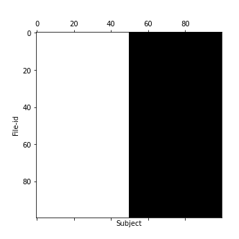
II-C1 Complete Columns (Figure 1(a))

The training set is sampled by randomly selecting complete columns in the utility matrix, that is, complete subject executions. The last selected column might be incomplete to meet the exact training ratio. This method respects the time constraints. It corresponds to a situation where the collaborative filtering method will predict the reproducibility of the subjects in the test set from the subjects in the training set.

II-C2 Complete Rows (Figure 1(b))

The training set is sampled by selecting complete rows in the utility matrix, that is, the first files produced by every execution. The last selected row might be incomplete to meet the exact training ratio. This method respects the time constraints. It corresponds to a situation where the processing of all the subjects is launched and interrupted before the execution is complete. The collaborative filtering method will then predict the reproducibility of the remaining files.

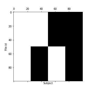
II-C3 Random Subjects – RS (Figure 1(c))

This method builds the training set by selecting the files from random subjects until the training ratio is reached. The file selected in a subject is the file with the lowest index in this subject that has not been already selected in the training set, which respects the time constraints.

II-C4 Random File Numbers (Uniform) – RFNU (Figure 1(d))

The number of files selected for every subject is randomly selected in a uniform distribution $U(\textit{a},\textit{b})$ , where b is set to the total number of files $N_{f}$ and a is set according to training ratio $\alpha$ as follows:

\begin{cases}\textit{a}=0&\text{if $\alpha\leq 0.5$ }\\ \textit{a}=(2\alpha-1)N_{f}&\text{if $\alpha>0.5$}\end{cases}

For $\alpha\leq 0.5$ , we ensure that the average number of selected files by subject is $\alpha N_{f}$ by sampling the number of files in every subject from $U(0,N_{f})$ with probability $2\alpha$ , and setting it to 0 otherwise. For $\alpha>0.5$ , this is ensured by the value of $a$ , which leads the average of U(a, b) to be $\alpha N_{f}$ .

II-C5 Random File Numbers (Triangular) – RFNT

The number of files selected for every subject is randomly selected in a triangular distribution $T(a,b,c)$ as in Figure 2. The mean of the distribution is $\frac{a+b+c}{3}$ . We set c to $N_{f}$ and we set a and b with the following two approaches.

Largest a (RFNTL, Figure 1(e))

a is set to the largest possible value, i.e., b, and b is set accordingly to ensure that the average of the distribution is $\alpha N_{f}$ . Two cases occur:

•

When $\alpha>1/3$ :

$\textit{a}=\textit{b}=\frac{3\alpha-1}{2}N_{f}$
•

When $\alpha\leq 1/3$ : $a=b=0$ , the number of files selected in every subject is sampled from $T(0,0,N_{f})$ with probability $3\alpha$ and set to 0 otherwise.

Smallest a (RFNTS, Figure 1(f))

a is set to the smallest possible value, i.e., 0, and b is set accordingly to ensure that the average of the distribution is $\alpha N_{f}$ . Three cases occur:

•

When $\alpha<1/3$ : $a=b=0$ , the number of files selected in every subject is sampled from $T(0,0,N_{f})$ with probability $3\alpha$ and set to 0 otherwise.
•

When $1/3\leq\alpha\leq 2/3$ :

$\textit{a}=0\quad;\quad\textit{b}=N_{f}(3\alpha-1)$
•

When $\alpha\geq 2/3$ : $b=N_{f}$ , the number of files selected in every subject is sampled from $T(0,N_{f},N_{f})$ with probability $3(1-\alpha)$ and set to $N_{f}$ otherwise.

As illustrated in Figures 1(e) and 1(f), the point of the RFNTL method is to guarantee that, for large enough values of $\alpha$ , all subjects will have at least a few files in the training set (no empty column), which is not the case for RFNU or RFNTS.

II-C6 Random Unreal (Figure 1(g))

The training set is sampled in a random uniform way, regardless of the file creation times. This method does not respect the time constraints in Equation 1: it will be used as a baseline for comparison.

In each method, we also included the first row of the matrix (first file of each subject) and a random column (all files of a random subject) to avoid cold start issues.

III Datasets

III-A Synthetic Dataset

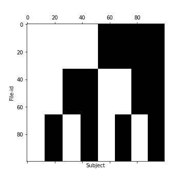
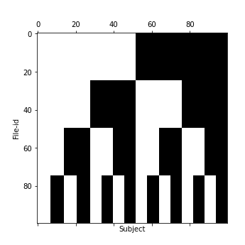
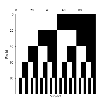
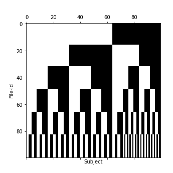
We generated synthetic matrices as shown in Figure 3. Each matrix has 100 files and 100 subjects of different types. Subjects of the same type behave identically and all types contain the same number of subjects $\pm$ 1. Such a decomposition by subject type corresponds to a situation where different subjects may have data of different nature, as is the case in the Human Connectome Project data [5] where not all the subjects have the same amount of images.

For subjects of a given type, the matrix consists of $log(n)$ blocks, where $n$ is the number of types. Blocks are defined with all the possible variation patterns: some types do not vary at all, while other ones vary between every block. Such patterns are meant to mimic the logic of data processing pipelines: each block of files represents the files produced at a given stage of the pipeline, which may or may not contain reproducibility errors depending on the subject type.

III-B Real Dataset

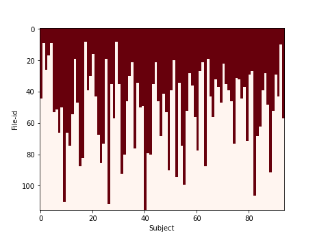
We processed a set S of 94 subjects randomly selected in the S500 HCP release¹¹1https://db.humanconnectome.org of the Human Connectome Project [12], in three execution conditions with different versions of the CentOS operating system (5.11, 6.8 and 7.2 – referred as C5, C6 and C7), using the PreFreesurfer and Freesurfer pipelines described in [12] and available on GitHub²²2https://github.com/Washington-University/Pipelines/releases/tag/v3.19.0. For each pipeline, we identified the set F of files produced for all subjects in all conditions. For each condition pair and each pipeline, we computed a binary reproducibility matrix U of size $|F|\times|S|$ , where $U_{i,j}$ is true if and only if file $i$ of subject $j$ was different in each condition. Rows of $U$ were ordered by ascending file modification time in a random subject in S.

Figure 4 shows the matrices for PreFreesurfer and Freesufer. The reproducibility of these pipelines varies across subjects, but most files behave consistently across all subjects, leading to complete black or white lines.

IV Results

We conducted two experiments for each reproducibility matrix, to evaluate the performance of our predictions using (1) ALS without biases, and (2) ALS with subject and file biases. We compare the performance of our sampling methods to (1) a dummy classifier that always predicts the value in the majority class and (2) the Random Unreal method, used as the baseline sampling technique. All reported values are averages over 5 repetitions. Due to sampling issues, it is possible that the actual training ratio obtained with some of the sampling methods does not exactly match the target one. We checked that the difference between the target and real training ratios was lower than 0.01. We used Spark’s ALS model as available in pyspark.ml, with 50 factors, a regularization parameter of 0.01, a maximum of 5 iterations and non negative constraints set to true. The code and data used to obtain the results are available through GitHub at https://github.com/big-data-lab-team/paper-reproducibility-collaborative-filtering.

IV-A Accuracy on Synthetic Data

IV-A1 ALS without Bias

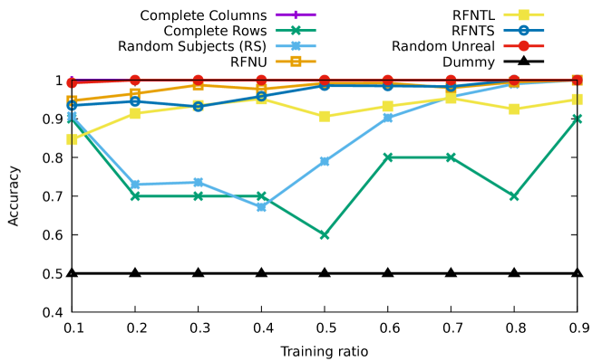
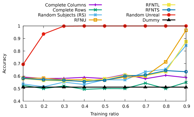
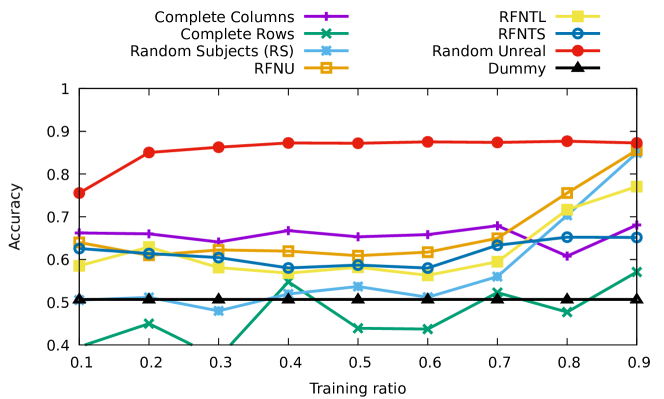
Figure 5 shows accuracy results for ALS without bias. By construction, the accuracy of the dummy classifier is close to 0.5 for all subject types. Random Unreal performs well for all subject types, which confirms that ALS is working correctly. All the other methods perform better than the dummy classifier, and their accuracy decreases as the number of subject types increases. However, only 3 methods can provide accuracy values above 0.85 for all subject types: Random Subjects (RS), RFNU and RFNTL. Surprisingly, RFNTS does not perform well for more than 2 subject types, even for $\alpha=0.9$ .

IV-A2 ALS with Bias

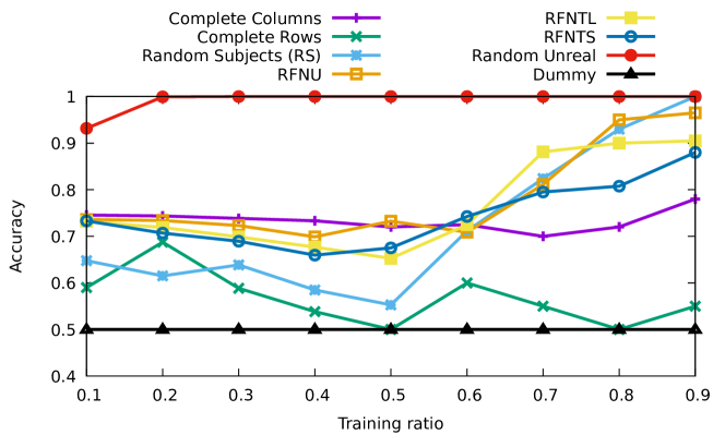
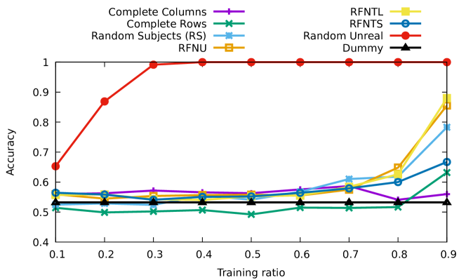
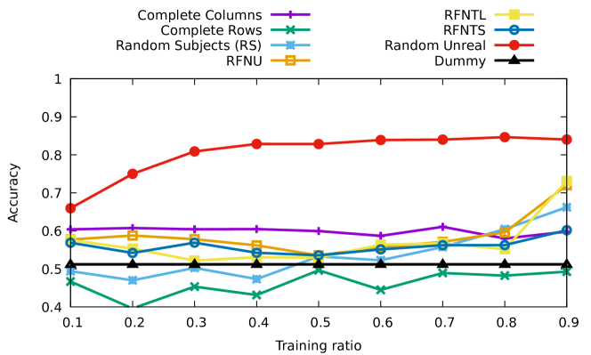
Figure 6 shows accuracy results for ALS with bias. RS, RFNU and RFNTL remain the methods that best compare to Random Unreal, but their accuracy is much lower than without biases. This is presumably due to the fact that file biases are all close to 0.5. In such a situation, biases are detrimental and should not be included.

IV-B Accuracy on Real Data

IV-B1 ALS without bias

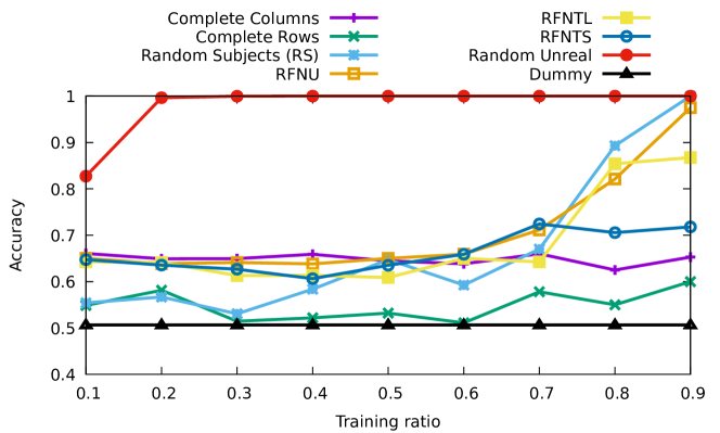
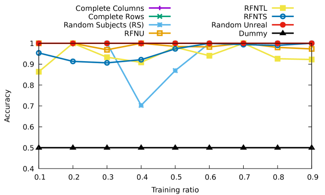
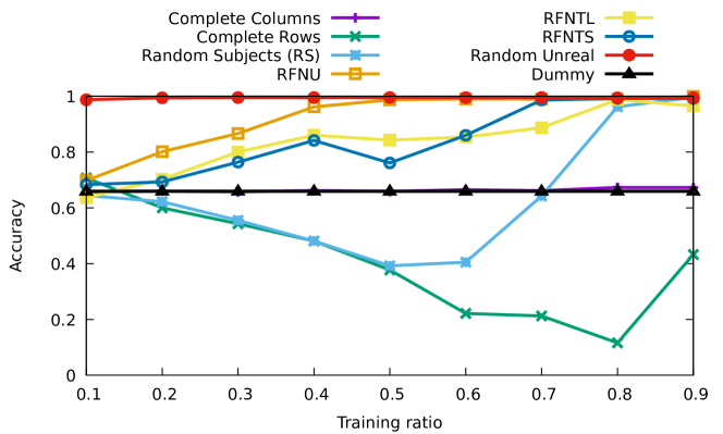
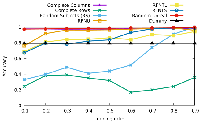
Figure 7 shows the accuracy for ALS without bias. Among the methods that performed well in the synthetic dataset, RFNU performs the best, with an accuracy higher than 0.95 for all datasets when the training ratio is larger than 0.5. Complete rows and complete columns do not reach the accuracy of the dummy classifier. Random Unreal has an accuracy close to 1, which shows that collaborative filtering works well on this dataset too.

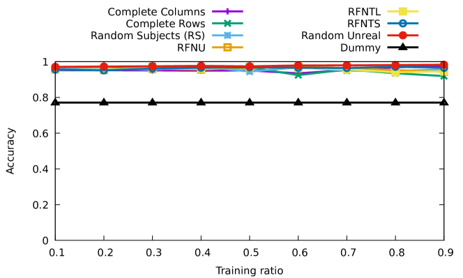
IV-B2 ALS with bias

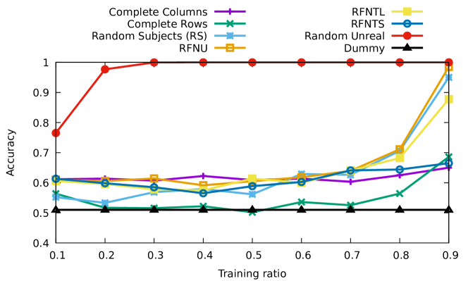
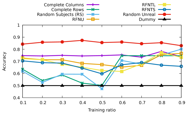
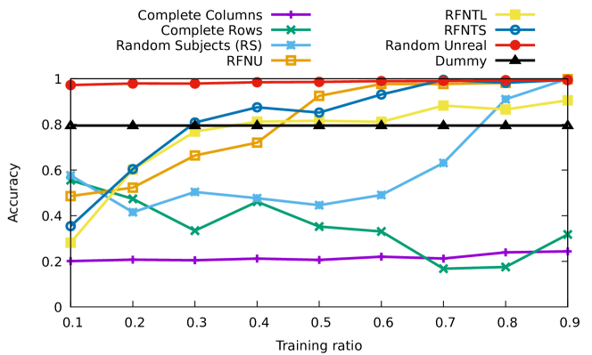
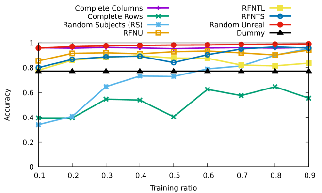
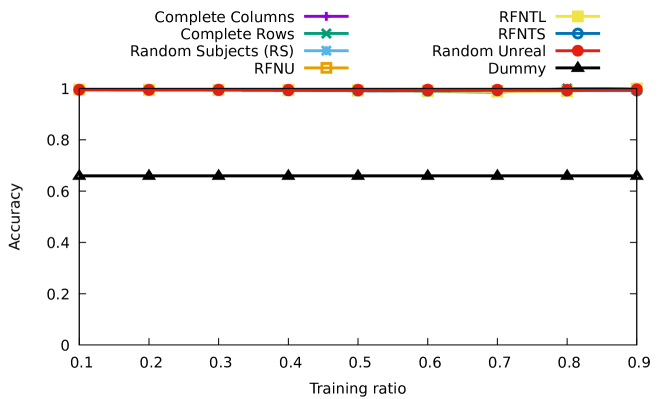
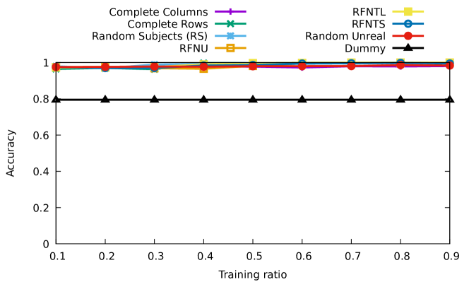
Figure 8 shows the accuracy for ALS with bias. From a training ratio of 0.5, all methods perform well for all datasets, except complete columns in Figure 8(b). All methods except RFNU, RFNTL and RFNTS also perform well for a training ratio lower than 0.5. Overall, the accuracy is much higher than without bias, due to the fact that the file biases are very strong. In the remainder, all the results are obtained using ALS without bias.

IV-C ROC analysis

Figure 9 compares the sampling methods in the ROC space, for a training ratio of 0.9, on the synthetic and Freesurfer dataset. The PreFreesurfer dataset is not included since specificity of RFNTL, RFNU, RS and complete rows is undefined at this training ratio (the test set only contains positive elements). The average sensitivity and specificity values are reported in Table I, which confirms that RFNU is the best performing method on average.

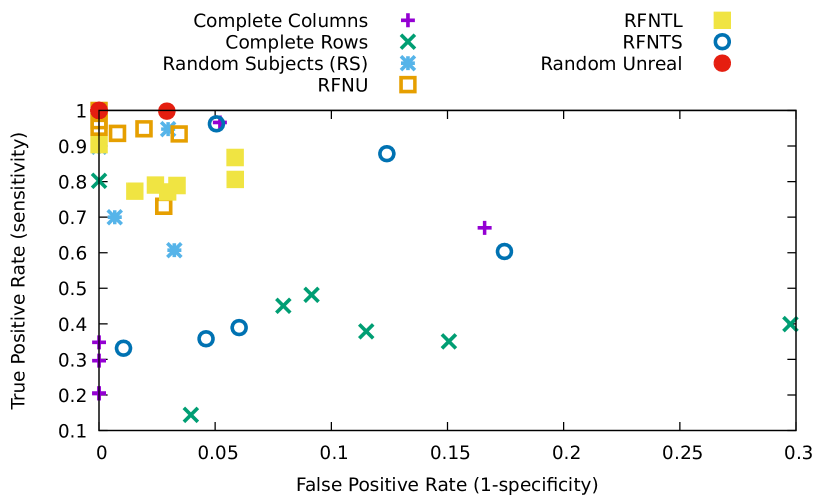
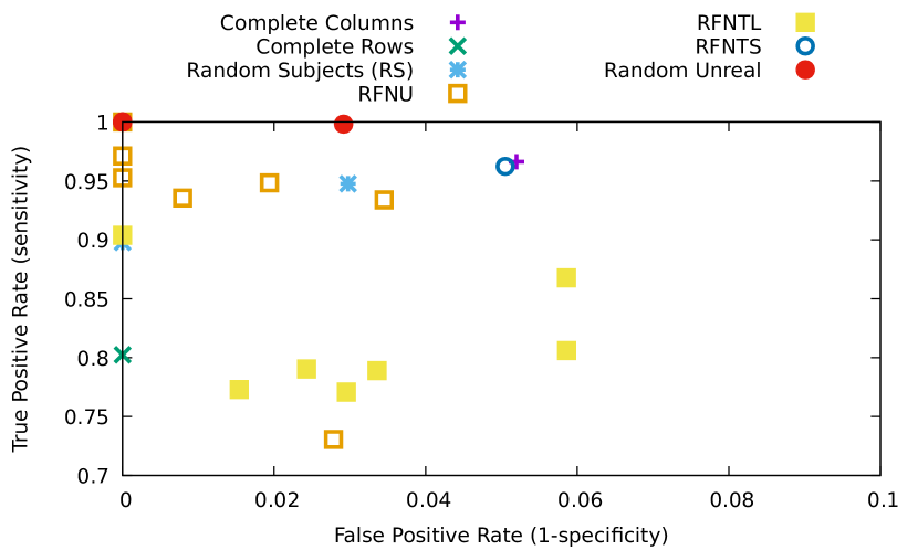
	Sensitivity	Specificity
Complete Columns	0.53	0.97
Complete Rows	0.43	0.89
Random Subjects	0.88	0.99
RFNU	0.92	0.99
RFNTL	0.81	0.97
RFNTS	0.65	0.93
Random Unreal	1	1

TABLE I: Average sensitivity and specificity for the synthetic datasets and Freesurfer (

\alpha=0.9

, ALS without bias).

IV-D Effect of the number of factors

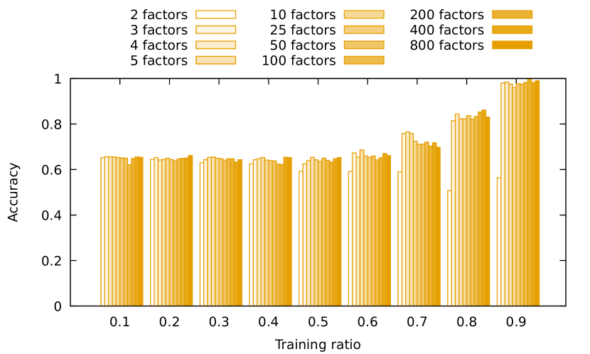
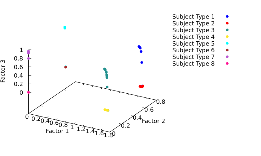
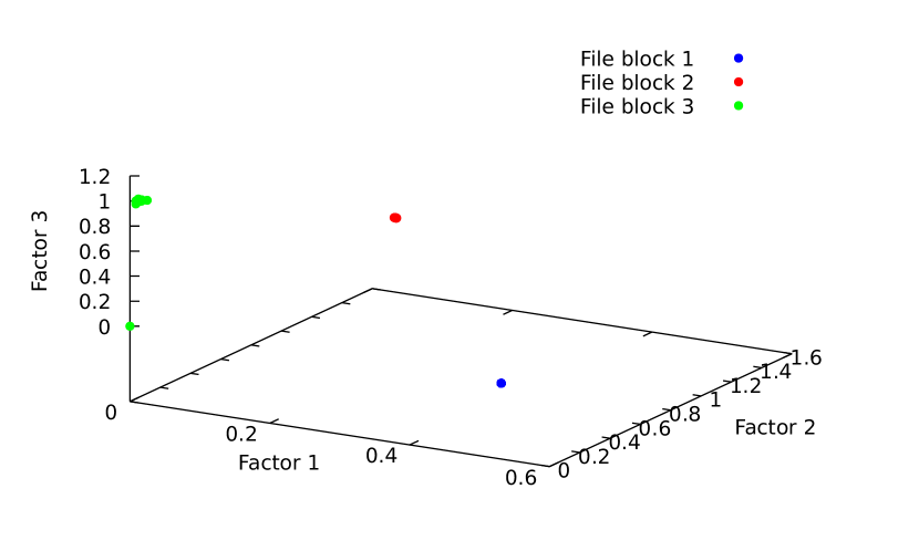
Figure 12 shows the effect of the number of factors used in the ALS optimization for the RFNU method and the synthetic dataset with 8 subject types (3 blocks of files). For training ratios greater than 0.5, the accuracy with 3 factors is substantially higher than with 2 factors. Beyond 3, the number of factors does not have any effect, which shows that the data is best explained by 3 factors. Figure 13 confirms that 3 factors are enough to separate the files of this dataset in 3 blocks, and the subjects in 8 types.

IV-E Effect of the maximum number of iterations

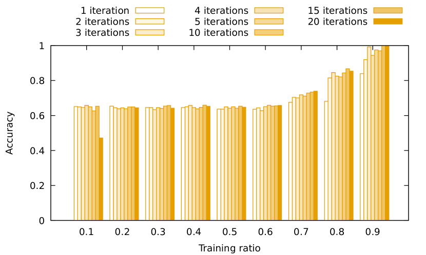
Figure 12 illustrates the effect of the number of iterations used in the ALS optimization, for the RFNU method and the synthetic dataset with 8 types. From a training ratio of 0.7, the number of iterations has a moderate effect on the accuracy. We used 5 iterations in our experiments, which only slightly degrades the accuracy compared to 15 or 20.

IV-F Prediction error localization

Figure 14 compares the prediction errors made by RFNU, RFNTL and RFNTS. The training set is represented in black (negatives) and white (positives), and the test set is in green (true positives), yellow (false negatives), gray (true negatives) and red (false positives). This representation provides insights regarding where, and perhaps why, prediction errors occur. At this training ratio, RFNU (Figure 14(a)) uniformly samples the number of files per subject between 0.8 $N_{f}$ and $N_{f}$ , which enables the training on the last files of the pipeline, while maintaining a low number of columns with a low training ratio. On the contrary, RFNTL (Figure 14(b)) samples the number of files per subject from 0.85 $N_{f}$ , but the probability to have a complete column is 0 (the one complete column in Figure 14(b) is the one included to prevent cold start issues), which leads to a “stripe” of prediction errors at the bottom of the matrix. RFNTS (Figure 14(c)) does not have this issue, as it includes many complete columns in the training set. However, it comes at the cost of several columns with a number of files lower than 60%: in such columns, the prediction is often entirely wrong, which explains the reduced accuracy compared to RFNU.

Figure 10 shows the RFNU results on the Freesurfer dataset for a training ratio of 0.6. The prediction error is localized (1) at the bottom of the matrix, which corresponds to the end of the execution, and (2) in the regions where file reproducibility varies across subjects, i.e., lines are not entirely black or entirely white. This is consistent with our expectations and confirms the validity of our results.

V Conclusion

While collaborative filtering, perhaps unsurprisingly, correctly predicts the missing values in a matrix modeling reproducibility evaluations, the usual random sampling method cannot be used in time-constrained processes. We proposed 6 sampling methods to address this issue, and we found that one of them, RFNU, performs better than the other ones on average. We explain that by the fact that RFNU builds the training set using a balanced mix of nearly complete and nearly empty columns, with a continuum of intermediate configurations. On the contrary, other methods, including RFNTL and RFNTS, bias the sampling toward complete or empty columns, which is sometimes detrimental to accuracy.

For datasets that are strongly dependent on row bias, such as the PreFreesurfer and Freesurfer ones, RFNU provides accuracy values consistently higher than 0.95 for training ratios higher than 0.5, even when biases are not included. For the synthetic dataset, RFNU still performs very well when biases are not included, but it does very poorly when biases are included. For this reason, we recommend to not include biases in the collaborative filtering optimization to solve this problem. Even though biases provide a slight accuracy improvement when datasets are strongly biased (constant lines in the matrix), they can also be very detrimental for more complex datasets such as the synthetic one used here.

From a practical standpoint, our study shows that reproducibility evaluations of the PreFreesurfer and Freesurfer pipelines can be conducted using only 50% of the files produced, with an accuracy above 95%. Potentially, this could reduce the computing time and storage required for such studies by a factor of 2. However, such studies could not be conducted by processing only half of the subjects entirely, which would correspond to the complete columns sampling method. Instead, the processing of all the subjects should be initiated and terminated in a random uniform way, assuming that files are uniformly produced throughout the execution. On more complex matrices, such as the synthetic dataset studied here, the training ratio required to get a 95% accuracy increases to 0.85.

Our study could be extended to real-valued reproducibility matrices instead of just binary ones. It is indeed common for file differences to be quantified using specific similarity measures or distances, such as the Levenshtein distance between strings, or the sum of squared distances among voxels of an image. Our sampling methods could be directly applied to real-valued matrices, and we expect our conclusions on the best-performing sampling method (RFNU) and the inclusion of biases in the model to remain valid.

Finally, the method described in this paper could possibly be used to predict the outcome of other time-constrained processes, for instance markers of chronic disease activity.

Acknowledgement

We thank Compute Canada for providing the compute and storage resources required for this study.

References

[1] R. D. Peng, “Reproducible research in computational science,” Science, vol. 334, no. 6060, pp. 1226–1227, 2011.
[2] M. Baker, “Is there a reproducibility crisis? A Nature survey lifts the lid on how researchers view the crisis rocking science and what they think will help,” Nature, vol. 533, no. 7604, pp. 452–455, 2016.
[3] E. H. Gronenschild, P. Habets, H. I. Jacobs, R. Mengelers, N. Rozendaal, J. Van Os, and M. Marcelis, “The effects of FreeSurfer version, workstation type, and macintosh operating system version on anatomical volume and cortical thickness measurements,” PloS one, vol. 7, no. 6, p. e38234, 2012.
[4] T. Glatard, L. B. Lewis, R. Ferreira da Silva, R. Adalat, N. Beck, C. Lepage, P. Rioux, M.-E. Rousseau, T. Sherif, E. Deelman et al., “Reproducibility of neuroimaging analyses across operating systems,” Frontiers in neuroinformatics, vol. 9, p. 12, 2015.
[5] D. C. Van Essen, S. M. Smith, D. M. Barch, T. E. Behrens, E. Yacoub, K. Ugurbil, W.-M. H. Consortium et al., “The WU-Minn Human Connectome Project: an overview,” Neuroimage, vol. 80, pp. 62–79, 2013.
[6] A. Bowring, C. Maumet, and T. Nichols, “Exploring the impact of analysis software on task fMRI results,” bioRxiv, p. 285585, 2018.
[7] D. Feng, C. Germain, and T. Glatard, “Efficient distributed monitoring with active collaborative prediction,” Future Generation Computer Systems, vol. 29, no. 8, pp. 2272–2283, 2013.
[8] J. Leskovec, A. Rajaraman, and J. D. Ullman, Mining of massive datasets. Cambridge university press, 2014.
[9] J. S. Breese, D. Heckerman, and C. Kadie, “Empirical analysis of predictive algorithms for collaborative filtering,” in Proceedings of the Fourteenth conference on Uncertainty in artificial intelligence. Morgan Kaufmann Publishers Inc., 1998, pp. 43–52.
[10] G. Linden, B. Smith, and J. York, “Amazon.com recommendations: Item-to-item collaborative filtering,” IEEE Internet computing, no. 1, pp. 76–80, 2003.
[11] Y. Koren, R. Bell, and C. Volinsky, “Matrix factorization techniques for recommender systems,” Computer, no. 8, pp. 30–37, 2009.
[12] M. F. Glasser, S. N. Sotiropoulos, J. A. Wilson, T. S. Coalson, B. Fischl, J. L. Andersson, J. Xu, S. Jbabdi, M. Webster, J. R. Polimeni et al., “The minimal preprocessing pipelines for the Human Connectome Project,” Neuroimage, vol. 80, pp. 105–124, 2013.