Fused Angles: A Representation of Body Orientation for Balance

Abstract

The parameterisation of rotations in three dimensional Euclidean space is an area of applied mathematics that has long been studied, dating back to the original works of Euler in the 18${}^{\text{th}}\mspace{-3.0mu}$ century. As such, many ways of parameterising a rotation have been developed over the years. Motivated by the task of representing the orientation of a balancing body, the fused angles parameterisation is developed and introduced in this paper. This novel representation is carefully defined both mathematically and geometrically, and thoroughly investigated in terms of the properties it possesses, and how it relates to other existing representations. A second intermediate representation, tilt angles, is also introduced as a natural consequence thereof.

I Introduction

Numerous ways of representing a rotation in three-dimensional Euclidean space have been developed and refined over the years. Many of these representations, also referred to as parameterisations, arose naturally from classical mathematics and have found widespread use in areas such as physics, engineering and robotics. Prominent examples of such representations include rotation matrices, quaternions and Euler angles. In this paper, a new parameterisation of the manifold of all three-dimensional rotations is proposed. This parameterisation, referred to as fused angles, was motivated by the analysis and control of the balance of bodies in 3D, and the shortcomings of the various existing rotation representations to describe the state of balance in an intuitive and problem-relevant way. More specifically, the advent of fused angles was to address the problem of representing the orientation of a body in an environment where there is a clear notion of what is ‘up’, defined implicitly, for example, through the presence of gravity. An orientation is just a rotation relative to some global fixed frame however, so fused angles can equally be used to represent any arbitrary three-dimensional rotation, much like Euler angles, for instance, can be used for both purposes. The shortcomings of Euler angles, however, that make them unsuitable for this balance-inspired task are discussed in detail in Section II-D.

When analysing the balance state of a body, such as for example of a humanoid robot, it is very helpful to be able to work with a parameterisation of the orientation that yields information about the components of the rotation within each of the three major planes, i.e. within the $\mathbf{x}\mathbf{y}$, $\mathbf{y}\mathbf{z}$ and $\mathbf{x}\mathbf{z}$ planes (see Fig. 1). These components of rotation can be conceptually thought of as a way of simultaneously quantifying the ‘amount of rotation’ about the individual axes. It is desirable for these components to each offer a useful geometric interpretation, and behave intuitively throughout the rotation space, most critically not sacrificing axisymmetry within the horizontal $\mathbf{x}\mathbf{y}$ plane by the introduction of a clear sequential order of rotations. The notion of fusing individual rotation components in a way that avoids such an order motivated the term ‘fused angles’. Quaternions, a common choice of parameterisation in computational environments, clearly do not address these requirements, as elucidated in Section II-C.

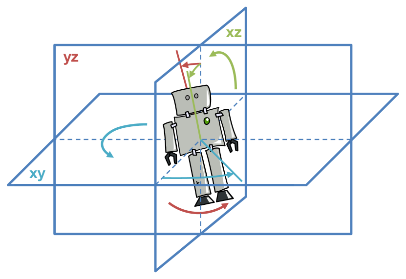
Figure 1: Fused angles are a way of decomposing a rotation into three concurrently acting components, in such a way that it gives insight into how rotated a body is in each of the three major planes.

The fused angles rotation representation has to date found a number of uses. Most recently in work published by the same authors, an attitude estimator was formulated that internally relied on the concept of fused angles [1]. The open source ROS software for the NimbRo-OP humanoid robot [2], developed by the University of Bonn, also relies on the use of fused angles, most notably in the areas of state estimation and walking. Furthermore, a Matlab and Octave library [3] targeted at the numerical and computational handling of all manners of three-dimensional rotation representations, including fused angles, has been released. This library is intended to serve as a common reference for the implementation in other programming languages of a wide range of conversion and computation functions. It is seen by the authors as a test bed to support the development of new rotation-related algorithms.

The convention that the global z-axis points in the ‘up’ direction relative to the environment is used in this paper. As mentioned previously, this accepted ‘up’ direction will almost always be defined as the antipodal direction of gravity. This ensures that definitions such as that of fused yaw make terminological sense in consideration of the true rotation of a body relative to its environment. All derived formulas and results could easily be rewritten using an alternative convention if this were to be desired.

The contribution of this paper lies in the introduction of the novel concept of fused angles for the representation of rotations. A further contribution is the concept of tilt angles (see Section III-A), an intermediary representation that emerges naturally from the derivation of the former.

II Review of Existing Rotation Representations

Many ways of representing 3D rotations in terms of a finite set of parameters exist. Different representations have different advantages and disadvantages, and which representation is suitable for a particular application depends on a wide range of considerations. Such considerations include:

• Ease of geometric interpretation, in particular in a form that is relevant to the particular problem,

• The range of singularity-free behaviour,

• Computational efficiency in terms of common operations such as rotation composition and vector rotation,

• Mathematical convenience, in terms of numeric and algebraic complexity and manipulability, and

• Algorithmic convenience, in the sense of a representation potentially possessing properties that can conveniently be exploited for a particular algorithm.

A wide range of existing rotation representations are reviewed in this section as a basis for comparison. Due to the dimensionality of the space of 3D rotations, a minimum of three parameters is required for any such representation. A representation with exactly three parameters is referred to as minimal, while other representations with a greater number of parameters are referred to as redundant.

II-A Rotation Matrices

A rotation can be represented as a linear transformation of coordinate frame basis vectors, expressed in the form of an orthogonal matrix of unit determinant. Due to the strong link between such transformation matrices and the theory of direction cosines, the name Direction Cosine Matrix is also sometimes used. The space of all rotation matrices is called the special orthogonal group $\text{SO}(3)$, and is defined as

$$\text{SO}(3)=\{R\in\mathbb{R}^{3\times 3}:R^{T}\!R=\mathbb{I},\,\det(R)=1\}.$$ (1)

Rotation of a vector $\mathbf{v}\in\mathbb{R}^{3}$ by a rotation matrix is given by matrix multiplication. For a rotation from coordinate frame {G} to {B}, we have that

$$\tensor*[^{G}_{B}]{R}{}=\begin{bmatrix}\tensor*[^{G}]{\mathbf{x}}{{}_{B}}&\mspace{-5.0mu}\tensor*[^{G}]{\mathbf{y}}{{}_{B}}&\mspace{-5.0mu}\tensor*[^{G}]{\mathbf{z}}{{}_{B}}\end{bmatrix}=\begin{bmatrix}\tensor*[^{B}]{\mathbf{x}}{{}_{G}}&\mspace{-5.0mu}\tensor*[^{B}]{\mathbf{y}}{{}_{G}}&\mspace{-5.0mu}\tensor*[^{B}]{\mathbf{z}}{{}_{G}}\end{bmatrix}^{T}\!\!,$$ (2)

where $\tensor*[^{G}]{\mathbf{y}}{{}_{B}}$, for example, is the column vector corresponding to the y-axis of frame {B}, expressed in the coordinates of frame {G}. The notation $\tensor*[^{G}_{B}]{R}{}$ refers to the relative rotation from {G} to {B}. With nine parameters, rotation matrices are clearly a redundant parameterisation of the rotation space. They are quite useful in that they are free of singularities and trivially expose the basis vectors of the fixed and rotated frames, but for many tasks they are not as computationally and numerically suitable as other representations.

II-B Axis-Angle and Rotation Vector Representations

By Euler’s rotation theorem [4], every rotation in the three-dimensional Euclidean space $\mathbb{R}^{3}$ can be expressed as a single rotation about some axis. As such, each rotation can be mapped to a pair $(\mathbf{\hat{u}},\theta)\in S^{2}\times\mathbb{R}$, where $\mathbf{\hat{u}}$ is a unit vector corresponding to the axis of rotation, and $\theta$ is the magnitude of the rotation. Note that $S^{2}=\{\mathbf{v}\in\mathbb{R}^{3}:\lVert\mathbf{v}\rVert=1\}$, the 2-sphere, is the set of all unit vectors in $\mathbb{R}^{3}$. A closely related concept is that of the rotation vector, given by $\mathbf{u}=\theta\mathbf{\hat{u}}$, which encodes the angle of rotation as the magnitude of the vector defining the rotation axis. Both the axis-angle and rotation vector representations suffer from a general impracticality of mathematical and numerical manipulation. For example, no formula for rotation composition exists that is more direct than converting to quaternions and back. The Simultaneous Orthogonal Rotations Angle (SORA) vector, a slight reformulation of the rotation vector concept in terms of virtual angular velocities and virtual time, was presented by Tomažič and Stančin in [5]. This formulation suffers from drawbacks similar to those of the rotation vector representation, which includes a discontinuity at rotations of 180^∘, and a general lack of geometric intuitiveness.

II-C Quaternions

The set of all quaternions $\mathbb{H}$, and the subset $\mathbb{Q}$ thereof of all quaternions that represent pure rotations, are defined as

$$\begin{split}\mathbb{H}&=\{q=(q_{0},\mathbf{q})\equiv(w,x,y,z)\in\mathbb{R}^{4}\},\\ \mathbb{Q}&=\{q\in\mathbb{H}:\lVert q\rVert=1\}.\end{split}$$ (3)

Quaternion rotations can be related to the axis-angle representation, and thereby visualised to some degree, using

$$q=(q_{0},\mathbf{q})=\bigl{(}\cos{\tfrac{\theta}{2}},\mathbf{\hat{u}}\sin{\tfrac{\theta}{2}}\bigr{)}\in\mathbb{Q},$$ (4)

where $(\mathbf{\hat{u}},\theta)\in S^{2}\times\mathbb{R}$ is any axis-angle rotation pair, and $q$ is the equivalent quaternion rotation. The use of quaternions to express rotations generally allows for very computationally efficient calculations, and is grounded by the well-established field of quaternion mathematics. A crucial advantage of the quaternion representation is that it is free of singularities. On the other hand however, it is not a one-to-one mapping of the special orthogonal group, as $q$ and $-q$ both correspond to the same rotation. The redundancy of the parameters also means that the unit magnitude constraint has to explicitly and sometimes non-trivially be enforced in numerical computations. Furthermore, no clear geometric interpretation of quaternions exists beyond the implicit relation to the axis-angle representation given in (4). For applications related to the balance of a body, where questions arise such as ‘how rotated’ a body is in total or within a particular major plane, the quaternion representation yields no direct insight.

II-D Euler Angles

A step in the right direction of understanding the different components of a rotation is the notion of Euler angles. In this representation, the total rotation is split into three individual elemental rotations, each about a particular coordinate frame axis. The three Euler angles $(\alpha,\beta,\gamma)$ describing a rotation are the successive magnitudes of these three elemental rotations. Many conventions of Euler angles exist, depending on the order in which the elemental axis rotations are chosen and whether the elemental rotations are taken to be intrinsic (about the rotating coordinate frame) or extrinsic (about the fixed coordinate frame). Extrinsic Euler angles can easily be mapped to their equivalent intrinsic Euler angles representations, and so the two types do not exhibit fundamentally different behaviour. If all three coordinate axes are used in the elemental rotations, the representation is alternatively known as Tait-Bryan angles, and the three parameters are referred to as yaw, pitch and roll, respectively. Tait-Bryan angles, although promising at first sight, do not suffice for the representation of the orientation of a body in balance-related scenarios. The main reasons for this are:

• The proximity of the gimbal lock singularity to normal working ranges, leading to unwanted artefacts due to increased local parameter sensitivity in a widened neighbourhood of the singularity,

• The fundamental requirement of an order of elemental rotations, leading to asymmetrical definitions of pitch and roll that do not correspond in behaviour, and

• The asymmetry introduced by the use of a yaw definition that depends on the projection of one of the coordinate axes onto a fixed plane, leading to unintuitive non-axisymmetric behaviour of the yaw angle.

The first listed point is a problem in real life, if for example a bipedal robot falls down, and thereby comes near the Euler angle singularity. As an example of the last of the listed points, consider the intrinsic ZYX Euler angles representation, recalling that the global z-axis points ‘upwards’ (see Section I). Consider a body in space, assumed to be in its identity orientation, and some arbitrary rotation of the body relative to its environment. It would be natural and intuitive to expect that the yaw of this relative rotation is independent of the chosen definition of the global x and y-axes. This is because the true rotation of the body is always the same, regardless of the essentially arbitrary choice of the global x and y-axes, and one would expect a well-defined yaw to be a property of the rotation, not the axis convention. This is not the case for ZYX Euler yaw however, as can be verified by counterexample with virtually any non-degenerate case. The yaw component of the fused angles representation, defined in Section III-A, can be proven to satisfy this property.

II-E Vectorial Parameterisations

Parameterisations are sometimes developed specifically to exhibit certain properties that can be exploited to increase the efficiency of an algorithm. A class of such generally more mathematical and abstract rotation representations is the family of vectorial parameterisations. Named examples of these include the Gibbs-Rodrigues parameters [6] and the Wiener-Milenković parameters [7], also known as the conformal rotation vector (CRV). Such parameterisations derive from mathematical identities such as the Euler-Rodrigues formula [8], and as such do not in general have any useful geometric interpretation, and find practical use in only very specific applications. Detailed derivations and analyses of vectorial parameterisations can be found in [6] and [7].

III Fused Angles

Fused angles were motivated by the lack of an existing 3D rotation formalism that naturally deals with the dissolution of a complete rotation into parameters that are specifically and geometrically relevant to the balance of a body, and that does not introduce order-based asymmetry in the parameters. None of the representations discussed in Section II satisfy this property. The unwanted artefacts in the existing notions of yaw (see Section II-D) also led to the need for a more suitable, stable and axisymmetric definition of yaw.

III-A Geometric Definition of Tilt Angles

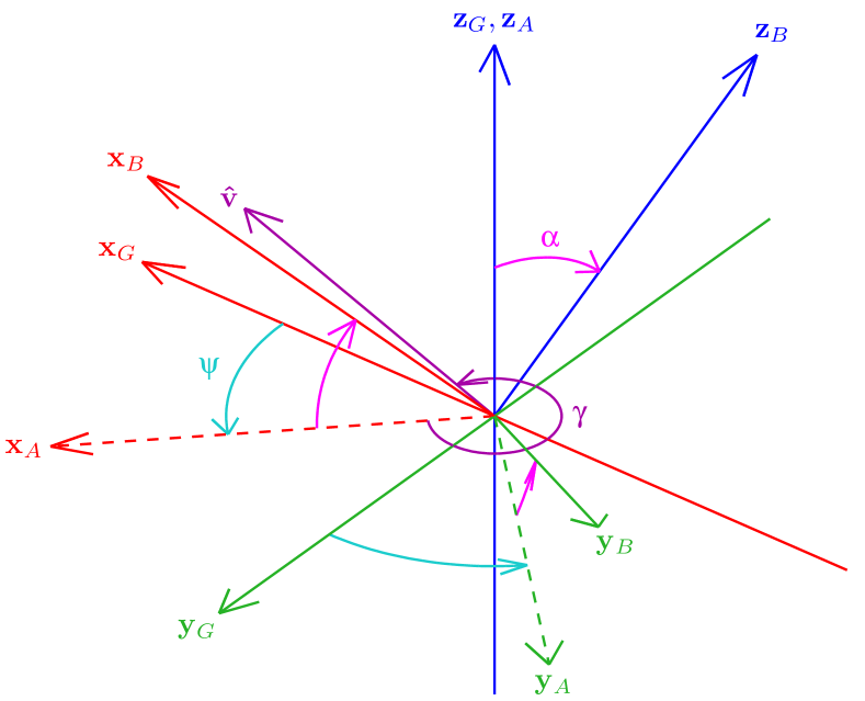
Figure 2: Definition of the tilt rotation and tilt angles parameters of the rotation from {G} to {B}. $\psi$ is the fused yaw, $\gamma$ is the tilt axis angle, $\alpha$ is the tilt angle and $\mathbf{\hat{v}}$ is the tilt axis. The intermediate frame {A} is constructed by rotating {B} such that $\tensor*{\mathbf{z}}{{}_{B}}$ rotates directly onto $\tensor*{\mathbf{z}}{{}_{G}}$.

We begin by defining an intermediate rotation representation, referred to as tilt angles. The tilt angles parameter definitions are illustrated in Fig. 2. Note that we follow the convention that, for example,

$$\tensor*[^{G}]{\mathbf{z}}{{}_{B}}=\bigl{(}\tensor*[^{G}]{z}{{}_{Bx}},\tensor*[^{G}]{z}{{}_{By}},\tensor*[^{G}]{z}{{}_{Bz}}\bigr{)}$$ (5)

denotes the unit vector corresponding to the positive z-axis of a frame {B}, expressed in the coordinates of a frame {G}. The absence of a coordinate basis qualifier, such as for example in the notation ‘$\tensor*{\mathbf{z}}{{}_{B}}$’, implies that a vector is by default expressed relative to the global fixed frame.

Let {G} denote the global fixed frame, defined with the convention that the global z-axis points upwards in the environment, as discussed in Section I. We define {B} to be the body-fixed coordinate frame. For an identity orientation of the body, the frames {G} and {B} should clearly coincide.

As $\tensor*{\mathbf{z}}{{}_{G}}$ and $\tensor*{\mathbf{z}}{{}_{B}}$ are vectors in $\mathbb{R}^{3}$, a rotation about an axis perpendicular to both vectors exists that maps $\tensor*{\mathbf{z}}{{}_{G}}$ onto $\tensor*{\mathbf{z}}{{}_{B}}$. Note that this is a different condition to mapping {G} onto {B}. We choose an axis-angle representation $(\mathbf{\hat{v}},\alpha)$ (see Section II-B) of this tilt rotation such that $\alpha\in[0,\pi]$. The angle $\alpha$ is referred to as the tilt angle of {B}, and the vector $\mathbf{\hat{v}}$ is referred to as the tilt axis of {B}. We define coordinate frame {A} to be the frame that results when we apply the inverse of the tilt rotation to {B}. By definition $\tensor*{\mathbf{z}}{{}_{A}}=\tensor*{\mathbf{z}}{{}_{G}}$, so it follows that $\mathbf{\hat{v}}$—and trivially also $\tensor*{\mathbf{x}}{{}_{A}}$—must lie in the $\tensor*{\mathbf{x}}{{}_{A}}\tensor*{\mathbf{y}}{{}_{A}}$ plane. The angle $\gamma$ about $\tensor*{\mathbf{z}}{{}_{A}}$ from $\tensor*{\mathbf{x}}{{}_{A}}$ to $\mathbf{\hat{v}}$ (see Fig. 2) is referred to as the tilt axis angle of {B}. It is easy to see that the tilt rotation from {A} to {B} is completely defined by the parameter pair $(\gamma,\alpha)$.

We now note that the rotation from {G} to {A} is one of pure yaw, that is, a pure z-rotation, and so define the angle $\psi$ about $\tensor*{\mathbf{z}}{{}_{G}}$ from $\tensor*{\mathbf{x}}{{}_{G}}$ to $\tensor*{\mathbf{x}}{{}_{A}}$ (see Fig. 2) as the fused yaw of {B}. It is important to note that the choice of using the x-axes in this definition of yaw is arbitrary, and a similar definition using the y-axes would be completely equivalent. The complete tilt angles representation of the rotation from {G} to {B} is now defined as

$$\tensor*[^{G}_{B}]{T}{}=(\psi,\gamma,\alpha)\in(-\pi,\pi]\times(-\pi,\pi]\times[0,\pi]\equiv\mathbb{T}.$$ (6)

The identity tilt angles rotation is given by $(0,0,0)\in\mathbb{T}$.

It can be seen from the method of construction that all rotations possess a tilt angles representation, although it is not always necessarily unique. Most notably, when $\alpha=0$, the $\gamma$ parameter can be arbitrary with no effect.

III-B Geometric Definition of Fused Angles

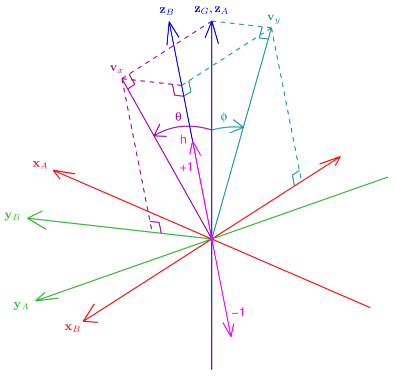
Figure 3: Definition of the fused angles parameters $(\theta,\phi,h)$ that describe the tilt rotation component of the rotation from {G} to {B}. {A} is the same intermediate frame as from the geometric definition of tilt angles (see Fig. 2). The $\tensor*{\mathbf{x}}{{}_{G}}$ and $\tensor*{\mathbf{y}}{{}_{G}}$ axes are not shown in the figure for visual simplicity. $\theta$ is the fused pitch, $\phi$ is the fused roll, $h$ is the hemisphere, $\tensor*{\mathbf{v}}{{}_{x}}$ is the projection of $\tensor*{\mathbf{z}}{{}_{G}}$ onto the $\tensor*{\mathbf{y}}{{}_{B}}\tensor*{\mathbf{z}}{{}_{B}}$ plane, and $\tensor*{\mathbf{v}}{{}_{y}}$ is the projection of $\tensor*{\mathbf{z}}{{}_{G}}$ onto the $\tensor*{\mathbf{x}}{{}_{B}}\tensor*{\mathbf{z}}{{}_{B}}$ plane. Geometrically it can be seen that $(\theta,\phi,h)$ depends only on the direction of $\tensor*{\mathbf{z}}{{}_{G}}$ relative to {B}, that is, $\tensor*[^{B}]{\mathbf{z}}{{}_{G}}$.

To remedy the possible ambiguity in the tilt angles parameters and work towards a more robust rotation representation, we introduce the concepts of fused pitch and fused roll. For reference, the relevant fused angles parameter definitions are illustrated in Fig. 3.

Let $\tensor*{\mathbf{v}}{{}_{x}}$ and $\tensor*{\mathbf{v}}{{}_{y}}$ be the projections of the $\tensor*{\mathbf{z}}{{}_{G}}$ vector onto the body-fixed $\tensor*{\mathbf{y}}{{}_{B}}\tensor*{\mathbf{z}}{{}_{B}}$ and $\tensor*{\mathbf{x}}{{}_{B}}\tensor*{\mathbf{z}}{{}_{B}}$ planes respectively. We define the fused pitch of {B} as the angle $\theta$ between $\tensor*{\mathbf{z}}{{}_{G}}$ and $\tensor*{\mathbf{v}}{{}_{x}}$, of sign $-\!\operatorname{sgn}\bigl{(}\tensor*[^{B}]{\mathbf{z}}{{}_{Gx}}\bigr{)}$. By logical completion, the magnitude of $\theta$ is taken to be $\tfrac{\pi}{2}$ if $\tensor*{\mathbf{v}}{{}_{x}}=\mathbf{0}$. We similarly define the fused roll of {B} as the angle $\phi$ between $\tensor*{\mathbf{z}}{{}_{G}}$ and $\tensor*{\mathbf{v}}{{}_{y}}$, of sign $\operatorname{sgn}\bigl{(}\tensor*[^{B}]{\mathbf{z}}{{}_{Gy}}\bigr{)}$. The magnitude of $\phi$ is taken to be $\tfrac{\pi}{2}$ if $\tensor*{\mathbf{v}}{{}_{y}}=\mathbf{0}$. Conceptually, fused pitch and roll can be thought of simply as the angles between $\tensor*{\mathbf{z}}{{}_{G}}$ and the $\tensor*{\mathbf{y}}{{}_{B}}\tensor*{\mathbf{z}}{{}_{B}}$ and $\tensor*{\mathbf{x}}{{}_{B}}\tensor*{\mathbf{z}}{{}_{B}}$ planes respectively. Note that this definition of fused pitch and roll is invariant to the entire body-fixed frame {B} being yawed, as one would expect.

From inspection of the geometric definitions, it can be seen that the fused pitch and roll only uniquely specify a tilt rotation up to the z-hemisphere, that is, whether $\tensor*{\mathbf{z}}{{}_{B}}$ and $\tensor*{\mathbf{z}}{{}_{G}}$ are mutually in the same hemisphere or not. To resolve this ambiguity, the hemisphere of a rotation (see Fig. 3) is defined as $\operatorname{sign}\bigl{(}\tensor*[^{B}]{\mathbf{z}}{{}_{Gz}}\bigr{)}\equiv\operatorname{sign}\bigl{(}\tensor*[^{G}]{\mathbf{z}}{{}_{Bz}}\bigr{)}$, where we define

$$\operatorname{sign}(x)=\begin{cases}1&\text{if $x\geq 0$},\\ 0&\text{if $x<0$}.\end{cases}$$ (7)

Note that $\operatorname{sign}$ differs to the normal definition of a sign function in that $\operatorname{sign}(0)=1$, whereas $\operatorname{sgn}(0)=0$. This modified sign function is used throughout the remainder of this paper wherever clear distinction from the normal sign function is required.

Using the concept of the hemisphere of a rotation, $(\theta,\phi,h)$ becomes a complete description of the tilt rotation component of a rotation. As such, together with the fused yaw $\psi$, the complete fused angles representation of the rotation from {G} to {B} can now be defined as

$$\tensor*[^{G}_{B}]{F}{} =(\psi,\theta,\phi,h)$$

$$\in(-\pi,\pi]\times[-\tfrac{\pi}{2},\tfrac{\pi}{2}]\times[-\tfrac{\pi}{2},\tfrac{\pi}{2}]\times\{-1,1\}\equiv\hat{\mathbb{F}}.$$ (8)

The identity fused angles rotation is given by $(0,0,0,1)\in\hat{\mathbb{F}}$. The $(\theta,\phi,h)$ triplet in (8) replaces the $(\gamma,\alpha)$ pair in (6) to define the tilt rotation component of a general rotation.

It can be observed from the geometric definitions above that the tilt rotation depends only on the direction of $\tensor*{\mathbf{z}}{{}_{G}}$ relative to frame {B}—that is, only on $\tensor*[^{B}]{\mathbf{z}}{{}_{G}}$. This, for example, means that the bottom row of the rotation matrix $\tensor*[^{G}_{B}]{R}{}$ (representing the rotation from {G} to {B}) can be completely identified with the tilt rotation component of that rotation. Interestingly, it can also be seen that the direction of $\tensor*{\mathbf{z}}{{}_{G}}$ relative to frame {B} is precisely what an accelerometer attached to the body would measure under the assumption of quasi-static conditions. In this way, accelerometer measurements can easily be mapped to measurements of $(\theta,\phi,h)$ and/or $(\gamma,\alpha)$.

III-C Mathematical Definition of Fused Angles and Tilt Angles

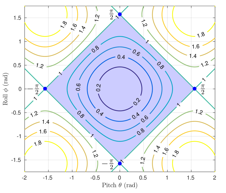
Figure 4: Level sets of the function $f_{s}(\theta,\phi)=\sin^{2}\!\theta+\sin^{2}\!\phi$, demonstrating that the sine sum criterion $f_{s}(\theta,\phi)\leq 1$ is equivalent to the simpler inequality $\lvert\theta\rvert+\lvert\phi\rvert\leq\tfrac{\pi}{2}$, indicated by the shaded region in the plot. The shaded region is the domain of $(\theta,\phi)$ for the fused angles representation.

Based on the given geometric definitions, the following expressions can be derived as an alternative mathematical definition of the tilt angles tilt rotation parameters:

$$\gamma =\operatorname{atan2}\bigl{(}-\tensor*[^{B}]{z}{{}_{Gx}},\tensor*[^{B}]{z}{{}_{Gy}}\bigr{)} \in(-\pi,\pi],$$ (9)

$$\alpha =\operatorname{acos}\bigl{(}\tensor*[^{B}]{z}{{}_{Gz}}\bigr{)} \in[0,\pi].$$ (10)

Similarly, alternative mathematical definitions for the fused angles tilt rotation parameters can be derived to be

$$\theta =\operatorname{asin}\bigl{(}-\tensor*[^{B}]{z}{{}_{Gx}}\bigr{)} \in[-\tfrac{\pi}{2},\tfrac{\pi}{2}],$$ (11)

$$\phi =\operatorname{asin}\bigl{(}\tensor*[^{B}]{z}{{}_{Gy}}\bigr{)} \in[-\tfrac{\pi}{2},\tfrac{\pi}{2}],$$ (12)

$$h =\operatorname{sign}\bigl{(}\tensor*[^{B}]{z}{{}_{Gz}}\bigr{)} \in\{-1,1\}.$$ (13)

The analysis for the fused yaw parameter is slightly more complex, but with the use of cases one can nonetheless mathematically define it as

$$\psi=\begin{cases}\operatorname{wrap}\bigl{(}\operatorname{atan2}\bigl{(}\tensor*[^{G}]{z}{{}_{Bx}},-\tensor*[^{G}]{z}{{}_{By}}\bigr{)}-\gamma\bigr{)}&\text{if $\alpha\neq 0$},\\ \operatorname{atan2}\bigl{(}\tensor*[^{G}]{x}{{}_{By}},\tensor*[^{G}]{x}{{}_{Bx}}\bigr{)}&\text{if $\alpha=0$},\end{cases}$$ (14)

where $\operatorname{wrap}$ is a function that wraps an angle to $(-\pi,\pi]$. An alternative mathematical definition for fused yaw, namely (36), is presented later in Section IV.

It can be seen from (11–13) and the unit norm condition that $\tensor*[^{B}]{\mathbf{z}}{{}_{G}}$ is given by a well-defined multivariate function $f_{z}:(\theta,\phi,h)\mapsto\tensor*[^{B}]{\mathbf{z}}{{}_{G}}$, described by

$$\tensor*[^{B}]{\mathbf{z}}{{}_{G}}=\Bigl{(}-\sin\theta,\sin\phi,h\sqrt{1-\sin^{2}\theta-\sin^{2}\phi}\Bigr{)},$$ (15)

where for obvious reasons we must have $\sin^{2}\theta+\sin^{2}\phi\leq 1$. This inequality is referred to by the authors as the sine sum criterion, and is precisely equivalent to

$$\lvert\theta\rvert+\lvert\phi\rvert\leq\tfrac{\pi}{2}.$$ (16)

Given that by definition $\theta,\phi\in[-\tfrac{\pi}{2},\tfrac{\pi}{2}]$, this equivalence can be seen by plotting the level sets of the multivariate function

$$f_{s}(\theta,\phi)=\sin^{2}\theta+\sin^{2}\phi,$$ (17)

and finding the region where $f_{s}(\theta,\phi)\leq 1$. The resulting plot is shown in Fig. 4. The domain of $f_{z}$ is the restriction of $[-\tfrac{\pi}{2},\tfrac{\pi}{2}]\times[-\tfrac{\pi}{2},\tfrac{\pi}{2}]\times\{-1,1\}$ to $\lvert\theta\rvert+\lvert\phi\rvert\leq\tfrac{\pi}{2}$, and the universal set of all fused angles, $\mathbb{F}$, is a similar restriction of $\hat{\mathbb{F}}$—that is, a restriction by the sine sum criterion.

III-D Visualisation of Fused Angles

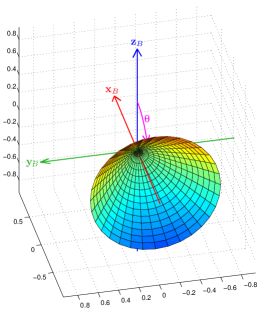
(a) Constant fused pitch cone for $\theta=50^{\circ}$

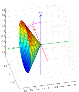
(b) Constant fused roll cone for $\phi=32^{\circ}$

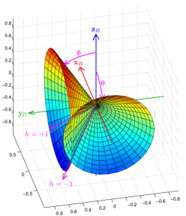
(c) Intersection of fused pitch and roll cones

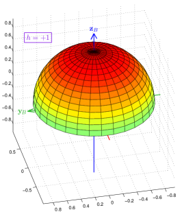
(d) Constant hemisphere locus for $h=+1$

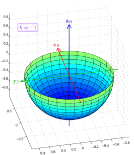
(e) Constant hemisphere locus for $h=-1$

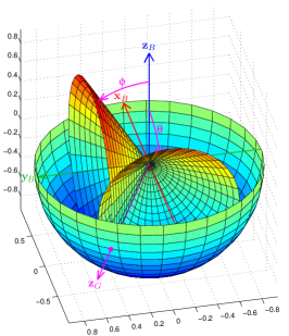
(f) Intersection of cones and hemisphere locus

Figure 5: Plots of the 3D locus of $\tensor*[^{B}]{\mathbf{z}}{{}_{G}}$ for (a) constant fused pitch $\theta$, (b) constant fused roll $\phi$, (d) constant hemisphere $h=+1$, and (e) constant hemisphere $h=-1$. (c) shows how loci of constant fused pitch and roll intersect at (at most) two points, illustrating how $(\theta,\phi)$ specifies $\tensor*[^{B}]{\mathbf{z}}{{}_{G}}$ up to two possible choices. (f) shows how intersecting again with the applicable hemisphere locus uniquely resolves $\tensor*[^{B}]{\mathbf{z}}{{}_{G}}$. Note that the locus of constant fused pitch in (a) is a cone with its opening facing out of the page, much like the opening of the cone of constant fused roll in (b) is facing towards the left.

The fused yaw parameter $\psi$ is best visualised precisely as defined and illustrated in Fig. 2. The remaining fused angles parameters, $(\theta,\phi,h)$, are also well visualised based on their geometric definition shown in Fig. 3, but can alternatively be envisioned as loci of $\tensor*[^{B}]{\mathbf{z}}{{}_{G}}$. Fig. 5 shows surface plots of the manifolds that are generated by independently taking the image of $f_{z}(\theta,\phi,h)$ for constant fused pitch $\theta$, fused roll $\phi$ and hemisphere $h$. The surfaces that result can be seen to be single-ended cones and hemispheres. It is important to note that the plots are in the body-fixed frame {B}, and not in the global fixed frame {G}. Fig. 5(c) and Fig. 5(f) show how combining specifications of $\theta$, $\phi$ and $h$ acts to resolve a unique $\tensor*[^{B}]{\mathbf{z}}{{}_{G}}$ based on the intersection of the various hemisphere and cone loci. The failure of two cones to intersect is precisely equivalent to a violation of the sine sum criterion, and hence an invalid specification of $\theta$ and $\phi$. The hemisphere parameter $h$ essentially decides which of the two cone intersections is used for $\tensor*[^{B}]{\mathbf{z}}{{}_{G}}$.

IV Conversions to Other Representations

Fused angles serve well in the analysis of body orientations, but even so, conversions to other representations are often required for mathematical computations such as rotation composition. The equations required for the conversion of the fused angles representation $F=(\psi,\theta,\phi,h)\in\mathbb{F}$ to and from tilt angles, rotation matrix and quaternion representations are presented in this section. Similar conversions are also provided for the tilt angles representation $T=(\psi,\gamma,\alpha)\in\mathbb{T}$. The proofs of the conversion equations are generally not difficult, but beyond the scope of this paper.

IV-1 Fused angles $\leftrightarrow$ Tilt angles

The yaw parameters $\psi$ of these two representations are equal, so the conversion from fused angles to tilt angles is completely summarised by

$$\gamma =\operatorname{atan2}(\sin\theta,\sin\phi),$$ (18)

$$\alpha =\operatorname{acos}\Bigl{(}h\sqrt{1-\sin^{2}\theta-\sin^{2}\phi}\Bigr{)},$$ (19)

where for numerical computation one may use the identity

$$1-\sin^{2}\theta-\sin^{2}\phi\equiv\cos(\theta+\phi)\cos(\theta-\phi).$$ (20)

We interestingly note from (19) that

$$\sin^{2}\theta+\sin^{2}\phi=\sin^{2}\alpha.$$ (21)

The conversion from tilt angles to fused angles is given by

$$\begin{aligned} \theta&=\operatorname{asin}(\sin\alpha\sin\gamma),\\ \phi&=\operatorname{asin}(\sin\alpha\cos\gamma),\end{aligned} \mspace{15.0mu}h =\begin{cases}1&\text{if $\alpha\leq\tfrac{\pi}{2}$,}\\ -1&\text{otherwise.}\end{cases}$$ (22)

IV-2 Tilt angles $\leftrightarrow$ Rotation matrix

Based on the geometric definition of tilt angles given in Section III-A, the rotation matrix equivalent to $T=(\psi,\gamma,\alpha)\in\mathbb{T}$ can be seen to be

$$R=\begin{bmatrix}c_{\gamma}c_{\beta}+c_{\alpha}s_{\gamma}s_{\beta}&s_{\gamma}c_{\beta}-c_{\alpha}c_{\gamma}s_{\beta}&s_{\alpha}s_{\beta}\\ c_{\gamma}s_{\beta}-c_{\alpha}s_{\gamma}c_{\beta}&s_{\gamma}s_{\beta}+c_{\alpha}c_{\gamma}c_{\beta}&-s_{\alpha}c_{\beta}\\ -s_{\alpha}s_{\gamma}&s_{\alpha}c_{\gamma}&c_{\alpha}\end{bmatrix}\!,$$ (23)

where $\beta=\psi+\gamma$, $s_{x}\equiv\sin{x}$ and $c_{x}\equiv\cos{x}$.

The inverse conversion from a rotation matrix $R$ to the corresponding tilt angles representation $T$ is given by

$$\gamma =\operatorname{atan2}(-R_{31},R_{32}), \alpha =\operatorname{acos}(R_{33}),$$ (24)

where the fused yaw $\psi$ is calculated using (26–27), as presented below for the fused angles case.

IV-3 Fused angles $\leftrightarrow$ Rotation matrix

The conversion of fused angles to a rotation matrix requires conversion via the tilt angles representation, using (18–19). Equation (23) can then be used with slight simplification as follows:

$$R=\begin{bmatrix}c_{\gamma}c_{\beta}+c_{\alpha}s_{\gamma}s_{\beta}&s_{\gamma}c_{\beta}-c_{\alpha}c_{\gamma}s_{\beta}&s_{\alpha}s_{\beta}\\ c_{\gamma}s_{\beta}-c_{\alpha}s_{\gamma}c_{\beta}&s_{\gamma}s_{\beta}+c_{\alpha}c_{\gamma}c_{\beta}&-s_{\alpha}c_{\beta}\\ -s_{\theta}&s_{\phi}&c_{\alpha}\end{bmatrix}\!.$$ (25)

The conversion from $R$ back to $F$ follows from (11–13). If $R_{m}=\max\{R_{11},R_{22},R_{33}\}$ and $R_{z}=1-R_{11}-R_{22}+R_{33}$, then the rotation matrix to fused angles conversion is most robustly given by the following:

$$\tilde{\psi}=\begin{cases}\operatorname{atan2}(R_{21}-R_{12},1+\operatorname{tr}(R))&\mspace{-2.0mu}\text{if $\operatorname{tr}(R)\geq 0$}\\ \operatorname{atan2}(R_{z},R_{21}-R_{12})&\mspace{-2.0mu}\text{if $R_{m}=R_{33}$}\\ \operatorname{atan2}(R_{32}+R_{23},R_{13}-R_{31})&\mspace{-2.0mu}\text{if $R_{m}=R_{22}$}\\ \operatorname{atan2}(R_{13}+R_{31},R_{32}-R_{23})&\mspace{-2.0mu}\text{if $R_{m}=R_{11}$}\end{cases}$$ (26)

$$\psi =\operatorname{wrap}(2\tilde{\psi}), \theta =\operatorname{asin}(-R_{31}),$$ (27)

$$\phi =\operatorname{asin}(R_{32}), h =\operatorname{sign}(R_{33}).$$ (28)

Although it is possible to construct a much simpler expression for $\psi$ using (14), this is not recommended due to the resulting numerical sensitivity near $\alpha=0$.

IV-4 Tilt angles $\leftrightarrow$ Quaternion

The conversion of a tilt angles rotation $T=(\psi,\gamma,\alpha)\in\mathbb{T}$ to the corresponding quaternion representation is robustly given by

$$q=(c_{\bar{\alpha}}c_{\bar{\psi}},s_{\bar{\alpha}}c_{\bar{\psi}+\gamma},s_{\bar{\alpha}}s_{\bar{\psi}+\gamma},c_{\bar{\alpha}}s_{\bar{\psi}}),$$ (29)

where $\bar{\alpha}=\tfrac{1}{2}\alpha$ and $\bar{\psi}=\tfrac{1}{2}\psi$. In combination with (36) for calculating the fused yaw $\psi$, the inverse conversion from quaternion $q$ to tilt angles $T$ is given by

$$\gamma =\operatorname{atan2}(wy-xz,wx+yz),$$ (30)

$$\alpha =\operatorname{acos}\bigl{(}2(w^{2}+z^{2})-1\bigr{)}.$$ (31)

IV-5 Fused angles $\leftrightarrow$ Quaternion

The conversion from fused angles to quaternions is robustly given by

$$q =\begin{cases}\dfrac{\tilde{q}_{p}}{\lVert\tilde{q}_{p}\rVert}&\text{if $h=1$},\\[8.00003pt] \dfrac{\tilde{q}_{n}}{\lVert\tilde{q}_{n}\rVert}&\text{if $h=-1$},\end{cases}$$ (32)

$$\tilde{q}_{p} =\bigl{(}c_{\bar{\psi}}C_{\alpha}^{+},s_{\phi}c_{\bar{\psi}}-s_{\theta}s_{\bar{\psi}},s_{\phi}s_{\bar{\psi}}+s_{\theta}c_{\bar{\psi}},s_{\bar{\psi}}C_{\alpha}^{+}\bigr{)},$$ (33)

$$\tilde{q}_{n} =\bigl{(}s_{\alpha}c_{\bar{\psi}},c_{\bar{\psi}+\gamma}C_{\alpha}^{-},s_{\bar{\psi}+\gamma}C_{\alpha}^{-},s_{\alpha}s_{\bar{\psi}}\bigr{)},$$ (34)

where $C_{\alpha}^{+}=1+c_{\alpha}$ and $C_{\alpha}^{-}=1-c_{\alpha}$. The respective quaternion norms are analytically given by

$$\lVert\tilde{q}_{p}\rVert =\sqrt{2C_{\alpha}^{+}}=2c_{\bar{\alpha}}, \lVert\tilde{q}_{n}\rVert =\sqrt{2C_{\alpha}^{-}}=2s_{\bar{\alpha}}.$$ (35)

Note that $\alpha$ does not need to be computed in order to evaluate (32–34), just $c_{\alpha}$ and $s_{\alpha}$. These can be obtained directly from (19) and (21). Using (27–29), the fused angles representation of a quaternion $q=(w,x,y,z)\in\mathbb{Q}$ can be shown to be

$$\psi =\operatorname{wrap}\bigl{(}2\operatorname{atan2}(z,w)\bigr{)}, \theta =\operatorname{asin}\bigl{(}2(wy-xz)\bigr{)},$$ (36)

$$h =\operatorname{sign}(w^{2}+z^{2}-\tfrac{1}{2}), \phi =\operatorname{asin}\bigl{(}2(wx+yz)\bigr{)}.$$ (37)

Note that this expression for $\psi$ is insensitive to the quaternion magnitude, and far more direct than an expression derived from (26) would be. In fact, (36) can conveniently be taken as the mathematical definition of fused yaw. Note that the angle wrapping of $\psi$ is at most by a single multiple of $2\pi$.

V Singularity Analysis

When examining rotation representations, it is important to identify and precisely quantify any singularities. Singularities are unavoidable in any minimal parameterisation, and may occur in the form of:

1. A rotation that cannot unambiguously be resolved into the required set of rotation parameters,

2. A rotation for which there is no equivalent parameterised representation that is unambiguous,

3. A rotation in the neighbourhood of which the sensitivity of the rotation to parameters map is unbounded.

The entries of a rotation matrix are a continuous function of the underlying rotation and lie in the interval $[-1,1]$. As such, from (27–28) and the continuity of the appropriately domain-restricted arcsine function, it can be seen that the fused pitch and fused roll are continuous over the entire rotation space. Furthermore, the hemisphere parameter of the fused angles representation is uniquely and unambiguously defined over the rotation space. As a result, despite its discrete and thereby technically discontinuous nature, the hemisphere parameter is not considered to be the cause of any singularities in the fused angles representation.

The fused yaw parameter, on the other hand, can be seen from (36) to have a singularity at $w=z=0$, due to the singularity of $\operatorname{atan2}$ at $(0,0)$. From (29), this condition can be seen to be precisely equivalent to $\alpha=\pi$, the defining equation of the set of all rotations by 180^∘ about axes in the $\mathbf{x}\mathbf{y}$ plane. The fused yaw singularity is a singularity of type (ii) and (iii) as per the characterisation given above, and corresponds to an essential discontinuity of the fused yaw map. Moreover, given any fused yaw singular rotation $R$, and any neighbourhood $U$ of $R$ in the rotation space $\text{SO}(3)$, for every $\psi\in(-\pi,\pi]$ there exists a rotation in $U$ with a fused yaw of $\psi$. Conceptually, the fused yaw singularity can be seen as being as ‘far away’ from the identity rotation as possible. This is by contrast not the case for Euler angles.

The tilt angles representation trivially has the same singularity in the fused yaw as the fused angles representation. In addition to this however, from (24), the tilt axis angle $\gamma$ also has a singularity when $R_{31}=R_{32}=0$. This corresponds to $\theta=\phi=0$, or equivalently, $\alpha=0$ or $\pi$—that is, either rotations of pure yaw, or rotations by 180^∘ about axes in the $\mathbf{x}\mathbf{y}$ plane. The tilt angle parameter $\alpha$ is continuous by (10) and the continuity of the arccosine function, and as such does not contribute any further singularities.

VI Results and Properties of Fused Angles

The fused angles representation possesses a remarkable number of subtle properties that turn out to be quite useful both mathematically and geometrically when working with them. One of these properties, relating to the axisymmetry of the representation, has already been stated without proof in Section II-D. Other—more complex—properties of fused angles, involving for example the matching of fused yaws between coordinate frames, were invoked in [1] to derive a computationally efficient algorithm to calculate instantaneous measurements of the orientation of a body from sensor data. Some of the more basic but useful properties of fused angles are presented in this section.

VI-A Fundamental Properties of Fused Angles

The following fundamental properties of fused angles hold, and form a minimum set of axiomatic conditions on the fused angles parameters.

• A pure x-rotation by $\beta\in[-\tfrac{\pi}{2},\tfrac{\pi}{2}]$ is given by the fused angles representation $(0,0,\beta,1)\in\mathbb{F}$.

• A pure y-rotation by $\beta\in[-\tfrac{\pi}{2},\tfrac{\pi}{2}]$ is given by the fused angles representation $(0,\beta,0,1)\in\mathbb{F}$.

• A pure z-rotation by $\beta\in(-\pi,\pi]$ is given by the fused angles representation $(\beta,0,0,1)\in\mathbb{F}$.

• Applying a pure z-rotation to an arbitrary fused angles rotation is purely additive in fused yaw.

Further fundamental properties of fused angles include:

• The parameter set $(\psi,\theta,\phi,h)\in\mathbb{F}$ is valid if and only if $\lvert\theta\rvert+\lvert\phi\rvert\leq\tfrac{\pi}{2}$, i.e. the sine sum criterion is satisfied.

• The parameter set $(\psi,\theta,\phi,h)\in\mathbb{F}$ can be put into standard form by setting $h=1$ if $\lvert\theta\rvert+\lvert\phi\rvert=\tfrac{\pi}{2}$, and $\psi=0$ if $\theta=\phi=0$ and $h=-1$ (i.e. $\alpha=\pi$).

• Two fused angles rotations are equal if and only if their standard forms are equal. Note that this identifies the $\alpha=\pi$ rotations due to the fused yaw singularity there.

VI-B Inverse of a Fused Angles Rotation

The fused angles representation of the inverse of a rotation is intricately linked to the fused angles parameters of a rotation. This is an almost unexpected result when compared to, for example, Euler angles, but follows trivially from the formulas and properties presented in this paper thus far. Consider a fused angles rotation $(\psi,\theta,\phi,h)$ with an equivalent tilt angles representation $(\psi,\gamma,\alpha)$. The parameters of the inverse rotation are given by

$$\psi_{inv} =-\psi,\mspace{12.0mu} \gamma_{inv} =\operatorname{wrap}(\psi+\gamma-\pi),$$ (38)

$$\alpha_{inv} =\alpha, \theta_{inv} =\operatorname{asin}\bigl{(}-\sin\alpha\sin(\psi+\gamma)\bigr{)},$$ (39)

$$h_{inv} =h, \phi_{inv} =\operatorname{asin}\bigl{(}-\sin\alpha\cos(\psi+\gamma)\bigr{)}.$$ (40)

The leftmost equation in (38) represents a remarkable property of fused yaw, one that other definitions of yaw such as ZYX Euler yaw do not satisfy. This property is referred to as negation through rotation inversion. It is worth noting that if a rotation has zero fused yaw, i.e. it is a pure tilt rotation, the inverse fused pitch and roll also satisfy the negation through rotation inversion property. That is,

$$\psi=0\;\iff\,\left\{\begin{aligned} \psi_{inv}&=-\psi,&\theta_{inv}&=-\theta,\\ h_{inv}&=h,&\phi_{inv}&=-\phi.\end{aligned}\right.$$ (41)

VI-C Characterisation of the Fused Yaw of a Quaternion

For rotations away from the singularity $\alpha=\pi$, that is, for rotations where the fused yaw is well-defined and unambiguous, inspection of (29) reveals that the z-component of a quaternion $q=(w,x,y,z)\in\mathbb{Q}$ is zero if and only if the fused yaw is zero. That is,

$$z=0\;\iff\;\psi=0.$$ (42)

Furthermore, it can be seen that the quaternion corresponding to the fused yaw of the rotation can be constructed by zeroing the x and y-components of $q$ and renormalising. That is,

$$q_{yaw}=\tfrac{1}{\sqrt{w^{2}+z^{2}}}(w,0,0,z).$$ (43)

This leads to one way of removing the fused yaw component of a quaternion—something that is a surprisingly common operation—using the expression

$$q_{tilt}=q_{yaw}^{*}q=\tfrac{1}{\sqrt{w^{2}+z^{2}}}\Bigl{(}wq+z(z,y,-x,-w)\Bigr{)}.$$ (44)

The fused yaw can also be computed using (36) and manually removed. Equations (43–44) fail only if $w=z=0$, which is precisely equivalent to $\alpha=\pi$, the fused yaw singularity.

VI-D Metrics over Fused Angles

For the design of rotation space trajectories and other purposes, it is useful to be able to quantify the distance between two rotations using a metric. Assuming two fused angle rotations $F_{1}$ and $F_{2}$, and their corresponding tilt angles representations $T_{1}=(\psi_{1},\gamma_{1},\alpha_{1})$ and $T_{2}=(\psi_{2},\gamma_{2},\alpha_{2})$, two naturally arising metrics [9] are ($\mspace{2.0mu}\cdot$ is the dot product):

$$d_{R}(F_{1},F_{2}) =\lVert\log(R_{1}^{T}\!R_{2})\rVert_{F}=2\operatorname{acos}\bigl{(}\lvert q_{1}\mspace{-3.0mu}\cdot q_{2}\rvert\bigr{)}=\theta,$$ (45)

$$d_{L}(F_{1},F_{2}) =1-\cos\bigl{(}\mspace{-2.0mu}\tfrac{\theta}{2}\mspace{-1.0mu}\bigr{)}=1-\lvert q_{1}\mspace{-3.0mu}\cdot q_{2}\rvert,$$ (46)

where $q_{1}$, $q_{2}$ are the corresponding quaternions, $\theta$ is the angle magnitude of the relative axis-angle rotation $(\mathbf{\hat{u}},\theta)$, and

$$q_{1}\mspace{-3.0mu}\cdot q_{2}=c_{\bar{\alpha}_{1}}c_{\bar{\alpha}_{2}}c_{\Delta\bar{\psi}}+s_{\bar{\alpha}_{1}}s_{\bar{\alpha}_{2}}c_{\Delta\bar{\psi}+\Delta\gamma},\vspace{0.3em}$$ (47)

where $\Delta\bar{\psi}=\tfrac{1}{2}(\psi_{1}-\psi_{2})$, $\,\Delta\gamma=\gamma_{1}-\gamma_{2}$, $\bar{\alpha}_{1}=\tfrac{1}{2}\alpha_{1}$ and$\bar{\alpha}_{2}=\tfrac{1}{2}\alpha_{2}$. Note that the Riemannian metric $d_{R}$ relates closely to spherical linear interpolation (slerp) [10], and as such serves as a metric of first choice. Actual computation of slerp is however still most efficiently done in the quaternion space. Direct interpolation of fused angles can give unexpected results in the general case, but for two rotations in the positive hemisphere it is a viable alternative, that for many applications will produce completely satisfactory results.

VII Conclusions

Two novel ways of parameterising a rotation were formally introduced in this paper. The main contribution of these, the fused angles representation, was developed to be able to describe a rotation in a way that yields insight into the components of the rotation in each of the three major planes of the Euclidean space. The second parameterisation that was introduced, tilt angles, was defined as an intermediate representation between fused angles and other existing representations. Nevertheless, the tilt angles representation proves to be geometrically, conceptually and mathematically useful. Many properties of the fused angles and tilt angles representations were derived, often in highlight of their simplicity, and the relations of these two representations to other commonly used representations were explicitly given. The computational efficiency of the two representations can be seen by inspection of our open-source implementation [3]. Due to their many special properties, fused angles fill a niche in the area of rotation parameterisation that is left vacant by alternative constructs such as Euler angles and quaternions, and are expected to yield valuable information and results, in particular in applications that involve balance.

References

- [1] P. Allgeuer and S. Behnke, “Robust sensor fusion for biped robot attitude estimation,” in Proceedings of 14th IEEE-RAS Int. Conference on Humanoid Robotics (Humanoids), Madrid, Spain, 2014.
- [2] P. Allgeuer, M. Schwarz, J. Pastrana, S. Schueller, M. Missura, and S. Behnke, “A ROS-based software framework for the NimbRo-OP humanoid open platform,” in Proceedings of 8th Workshop on Humanoid Soccer Robots, IEEE-RAS Int. Conference on Humanoid Robots, Atlanta, USA, 2013.
- [3] P. Allgeuer. (2014, Oct) Matlab/Octave Rotations Library. [Online]. Available: https://github.com/AIS-Bonn/matlab_octave_rotations_lib/
- [4] B. Palais, R. Palais, and S. Rodi, “A disorienting look at Euler’s theorem on the axis of a rotation,” The American Mathematical Monthly, pp. 892–909, 2009.
- [5] S. Tomažič and S. Stančin, “Simultaneous orthogonal rotations angle,” Electrotechnical Review, no. 78, pp. 7–11, 2011.
- [6] O. Bauchau and L. Trainelli, “The vectorial parameterization of rotation,” Nonlinear Dynamics, vol. 32, no. 1, pp. 71–92, 2003.
- [7] L. Trainelli and A. Croce, “A comprehensive view of rotation parameterization,” in Proceedings of ECCOMAS, 2004.
- [8] J. Argyris, “An excursion into large rotations,” Computer Methods in Applied Mechanics and Engineering, vol. 32, pp. 85–155, 1982.
- [9] D. Huynh, “Metrics for 3D rotations: Comparison and analysis,” J. of Math. Imaging and Vision, vol. 35, no. 2, pp. 155–164, 2009.
- [10] K. Shoemake, “Animating rotation with quaternion curves,” in ACM SIGGRAPH computer graphics, vol. 19, no. 3, 1985, pp. 245–254.