Photometric Depth Super-Resolution

Abstract

This study explores the use of photometric techniques (shape-from-shading and uncalibrated photometric stereo) for upsampling the low-resolution depth map from an RGB-D sensor to the higher resolution of the companion RGB image. A single-shot variational approach is first put forward, which is effective as long as the target’s reflectance is piecewise-constant. It is then shown that this dependency upon a specific reflectance model can be relaxed by focusing on a specific class of objects (e.g., faces), and delegate reflectance estimation to a deep neural network. A multi-shot strategy based on randomly varying lighting conditions is eventually discussed. It requires no training or prior on the reflectance, yet this comes at the price of a dedicated acquisition setup. Both quantitative and qualitative evaluations illustrate the effectiveness of the proposed methods on synthetic and real-world scenarios.

1 Introduction

	Approach		SfS (Section 3)		SfS + reflectance learning (Section 4)		UPS (Section 5)
	Required data		1 RGB-D frame		1 RGB-D frame + training dataset		$n\geq 4$ RGB-D frames
	Albedo		Piecewise-constant		Learned (e.g., faces)		Arbitrary
Rucksack
Face 1
Tabletcase
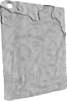
	$\mathbf{I}$	${z^{0}}$	${\bm{\rho}}$	$z$	${\bm{\rho}}$	$z$	${\bm{\rho}}$	$z$

Figure 1: Photometric depth super-resolution of a low-resolution depth map $z^{0}$ to the higher resolution of the companion image $\mathbf{I}$ (first column, Rucksack and Face 1 datasets were acquired using an Intel Realsense D415, and Tabletcase using an Asus Xtion Pro Live). Second column: shape-from-shading (SfS) recovers high-resolution albedo (${\bm{\rho}}$) and depth ($z$) from a single RGB-D frame, assuming piecewise-constant albedo. If this assumption is not satisfied (e.g., Face 1 and Tabletcase), shape estimation deteriorates. Third column: this can be circumvented by learning reflectance, an approach which is efficient as long as the target resembles the training data (here, training was carried out on human faces). Fourth column: uncalibrated photometric stereo (UPS) requires no training and handles arbitrary albedo, but it requires $n\geq 4$ input frames acquired under varying illumination. See Section 6 in the supplementary material for additional comparisons.

RGB-D sensors have become very popular for 3D-reconstruction, in view of their low cost and ease of use. They deliver a colored point cloud in a single shot, but the resulting shape often misses thin geometric structures. This is due to noise, quantisation and, more importantly, the coarse resolution of the depth map. In comparison, the quality and resolution of the companion RGB image are substantially better. For instance, the Asus Xtion Pro Live device delivers $1280\times 1024$ RGB images, but only up to $640\times 480$ depth maps. The depth map thus needs to be up-sampled to the same resolution of the RGB image, and the latter could be analysed photometrically to reveal fine-scale details.

However, super-resolution of a solitary depth map without additional contraints is an ill-posed problem, and retrieving geometry from either a single color image (shape-from-shading) or from a sequence of color images acquired under unknown, varying lighting (uncalibrated photometric stereo) is another ill-posed problem. The present study explores the resolution of both these ill-posedness issues by jointly performing depth super-resolution and photometric 3D-reconstruction. We call this combined approach photometric depth super-resolution.

The choice of jointly solving both these classic inverse problems is motivated by the observation that ill-posedness in depth super-resolution and in photometric 3D-reconstruction have different peculiarities and origins. In depth super-resolution, constraints on high-frequency shape variations are missing (there exist infinitely many ways to interpolate between two measurements), while low-frequency (e.g., concave-convex or bas-relief) ambiguities arise in photometric 3D-reconstruction. Therefore, the low-frequency geometric information necessary to disambiguate photometric 3D-reconstruction should be extracted from the low-resolution depth measurements and, symmetrically, the high-resolution photometric clues in the RGB data should provide the high-frequency information required to disambiguate depth super-resolution. One hand thus washes the other: ill-posedness in depth super-resolution is fought using photometric 3D-reconstruction, and vice-versa.

As we shall see in Section 2, the photometric depth super-resolution problem comes down to simultaneously inferring high-resolution depth and reflectance maps, given the low-resolution depth and the high-resolution RGB images. As depicted in Figure 1, this study explores three different strategies for such a task. The rest of this paper discusses them by increasing order of efficiency which, unfortunately, is inversely proportional to the amount of required resources. 1) If the available resources consist of a single RGB-D frame, then a variational approach to shape-from-shading can be followed. This approach, presented in Section 3, has no particular requirement in terms of acquisition setup or offline processing, yet it is effective only as long as the surface’s reflectance is piecewise-constant. 2) Section 4 then discusses a solution for eliminating this dependency upon a specific reflectance model. Pre-training a neural network for reflectance estimation allows to handle surfaces with more complex reflectance within the same variational framework. Yet, additional resources are required for offline training and the target has to resemble the objects used in the training phase (we thus focus in this section on human faces). 3) If multiple pairs of images can be acquired from the same viewing angle but under varying lighting, then one can resort to uncalibrated photometric stereo. This last strategy, discussed in Section 5, requires neither an assumption on the reflectance, nor offline training for a specific class of objects. However, it requires capturing more data online. Section 6 eventually recalls the main conclusions of this study and suggests future research directions.

2 Problem Statement

A generic RGB-D sensor is considered, which consists of a depth sensor and an RGB camera with parallel optical axes and optical centers lying on a plane orthogonal to these axes (see Figure 2). The images of the surface on the focal planes of the depth and the color cameras are denoted respectively by $\Omega_{LR}\subset\mathbb{R}^{2}$ and $\Omega_{HR}\subset\mathbb{R}^{2}$. In a single shot, the RGB-D sensor provides two 2D-representations of the surface:

• A geometric one, taking the form of a mapping ${z^{0}}:\,\Omega_{LR}\to\mathbb{R}$ between pixels in $\Omega_{LR}$ and the depth of their conjugate 3D-points on the surface;

• A photometric one, taking the form of a mapping $\mathbf{I}:\,\Omega_{HR}\to\mathbb{R}^{3}$ between pixels in $\Omega_{HR}$ and the radiance (relatively to the red, green and blue channels of the color camera) of their conjugate 3D-point.

In real-world scenarios, the sets $\Omega_{LR}$ and $\Omega_{HR}$ are discrete, and the cardinality $\left|\Omega_{LR}\right|$ of $\Omega_{LR}$ is lower than that $\left|\Omega_{HR}\right|$ of $\Omega_{HR}$. To obtain the richest surface representation, one should thus project the depth measurements ${z^{0}}$ from $\Omega_{LR}$ to $\Omega_{HR}$, i.e. estimate a new, high-resolution depth map $z:\,\Omega_{HR}\to\mathbb{R}$. To this end, we next introduce constraints arising from depth super-resolution and from photometric 3D-reconstruction.

Figure 2: Geometric setup. Depth measurements ${z^{0}}$ are available over a low-resolution set $\Omega_{LR}$, and color measurements $\mathbf{I}$ over a high-resolution set $\Omega_{HR}$. Photometric depth super-resolution consists in estimating a high-resolution depth map $z$ out of these geometric and photometric measurements, which are connected through the surface normals $\mathbf{n}_{{z,\nabla z}}$, see Equations (32) to (35).

2.1 Geometric and Photometric Constraints

Given the assumptions above on the alignment of the sensors, and neglecting occlusions, the low-resolution depth map $z^{0}$ can be considered as a downsampled version of the sought high-resolution one $z$, after warping and averaging:

$${z^{0}}=Kz+\eta_{z},$$ (1)

with $\eta_{z}$ the realisation of a stochastic process representing measurement errors and quantisation, and $K$ a non-invertible injective linear operator combining warping, blurring and downsampling [1], which can be calibrated beforehand [2]. Solving (32) in terms of the high-resolution depth map $z$ constitutes the depth super-resolution problem, which requires additional assumptions on the smoothness of the observed surface. In this work, the latter is assumed regular, i.e. the normal to the surface exists in every visible point. Denoting by $f>0$ the focal length of the color camera, and by $\mathbf{p}:\,\Omega_{HR}\to\mathbb{R}^{2}$ the field of pixel coordinates with respect to its principal point (blue reference coordinates system in Figure 2), the surface normal is defined as the following $\Omega_{HR}\to\mathbb{S}^{2}\subset\mathbb{R}^{3}$ field of unit-length vectors (see e.g., [3]):

$$\mathbf{n}_{z,\nabla z}=\frac{1}{\sqrt{\left|f\,\nabla z\right|^{2}+\left(-z-\mathbf{p}^{\top}\nabla z\right)^{2}}}\begin{bmatrix}f\,\nabla z\\ -z-\mathbf{p}^{\top}\nabla z\end{bmatrix}.$$ (2)

We further assume that the surface is Lambertian and lit by a collection of infinitely-distant point light sources. Lighting can then be represented in a compact manner using first-order spherical harmonics, see [4, 5] and Section 2.1 in the supplementary material. The irradiance in channel $\star\in\{R,G,B\}$ then writes

$$\mathbf{I}=\mathbf{l}^{\top}\underbrace{\begin{bmatrix}\mathbf{n}_{z,\nabla z}\\ 1\end{bmatrix}}_{:=\mathbf{m}_{z,\nabla z}}{\bm{\rho}}+{\bm{\eta}_{\mathbf{I}}},$$ (3)

with ${\bm{\eta}_{\mathbf{I}}}:\,\Omega_{HR}\to\mathbb{R}^{3}$ the realisation of a stochastic process standing for noise, quantisation and outliers, $\mathbf{l}\in\mathbb{R}^{4}$ the “light vector”, ${\bm{\rho}}:\,\Omega_{HR}\to\mathbb{R}^{3}$ the albedo (Lambertian reflectance) map and $\mathbf{m}_{z,\nabla z}:\,\Omega_{HR}\to\mathbb{R}^{4}$ a normal-dependent vector field. Solving (35) in terms of the high-resolution depth map $z$ constitutes the photometric 3D-reconstruction problem, where reflectance ${\bm{\rho}}$ and lighting $\mathbf{l}$ represent hidden variables to estimate.

Photometric depth super-resolution aims at inferring $z$ out of ${z^{0}}$ and $\mathbf{I}$, while ensuring consistency with the super-resolution constraint in (32) and with the photometric one in (35). Before elaborating on three strategies for solving this problem, let us first review related works.

2.2 Related Works

Single depth image super-resolution requires solving Equation (32) in terms of the high-resolution depth map $z$. Since $K$ is not invertible, this is an ill-posed problem: there exist infinitely many choices for interpolating between observations, cf. Section 2.2 in the supplementary material. Disambiguation can be carried out by adding observations obtained from different viewing angles [6, 7, 8]. In the more challenging case of a single viewing angle, a smoothness prior on the high-resolution depth map can be added and a variational approach can be followed [1]. One may also resort to machine learning techniques relying on a dictionary of low- and high-resolution depth or edge patches [9, 10]. Such a dictionary can even be constructed from a single depth image by looking for self-similarities [11, 12]. Nevertheless, learning-based depth super-resolution methods remain prone to over-fitting [13], which can be avoided by combining the respective merits of machine learning and variational approaches [14, 15].

Shape-from-shading [16, 17, 18, 19] is another classic inverse problem which aims at inferring shape from a single image of a scene, by inverting an image formation model such as (35). Common numerical strategies for this task include variational [20, 21] and PDE methods [22, 23, 24, 25]. However, even when reflectance and lighting are known, shape-from-shading is still ill-posed due to the underlying concave $/$ convex ambiguity, cf. Section 2.2 in the supplementary material. Obviously, even more ambiguities arise under more realistic lighting and reflectance assumptions: any image can be explained by a flat shape illuminated uniformly but painted in a complex manner, by a white and frontally-lit surface with a complex geometry, or by a white planar surface illuminated in a complex manner [26]. Shape-from-shading under uniform reflectance but natural lighting has been studied [27, 28, 29, 30], but the case with unknown reflectance requires the introduction of additional priors [31]. This can be avoided by actively controlling the lighting, a variant of shape-from-shading known as photometric stereo which allows to estimate both shape and reflectance [32]. The problem with uncalibrated lighting is however ill-posed: it can be solved only up to a linear ambiguity [33] which, assuming integrability of the normals, reduces to a generalised bas-relief (GBR) one under directional lighting [34], and to a Lorentz one under natural lighting [35]. Resolution of such ambiguities by resorting to additional priors [36, 37, 38], extensions to non-Lambertian reflectance [39] and natural illumination [40] remain active research topics for which public benchmarks exist [41]. Recent developments in this field include PDE-based variational methods [42] and machine learning solutions [43, 44].

Shape-from-shading has recently gained new life with the emergence of RGB-D sensors. Indeed, the rough depth map can be used as prior to “guide” shape-from-shading and thus circumvent its ambiguities. This has been achieved in both the multi-view [45, 46, 47] and the single-shot [48, 49, 50, 51, 52, 53] cases. Still, the resolutions of the input image and depth map are assumed equal, and the same holds for approaches resorting to photometric stereo instead of shape-from-shading [54, 55, 56, 57]. In fact, depth super-resolution and photometric 3D-reconstruction have been widely studied, but rarely together. Several methods were proposed to coalign the depth edges in the super-resolved depth map with edges in the high-resolution color image [58, 59, 2, 60, 61, 62], but such approaches only consider sparse color features and may thus miss thin geometric structures. Some authors super-resolve the photometric stereo results [63], and others generate high-resolution images using photometric stereo [64], but none employ low-resolution depth clues except those of [65], who combine calibrated photometric stereo with structured light sensing. However, this involves a non-standard setup and careful lighting calibration, and reflectance is assumed to be uniform. Such issues are circumvented in the building blocks [66] and [67] of this study, which deal with photometric depth super-resolution based on, respectively, shape-from-shading and photometric stereo. Let us present the former approach, which is a single-shot solution to photometric depth super-resolution based on a variational approach to shape-from-shading.

3 Single-shot Depth Super-resolution using Shape-from-shading

In this section, the input data consists of a single RGB-D frame, i.e. a high-resolution image $\mathbf{I}$ and a low-resolution depth map ${z^{0}}$. To obtain a high-resolution depth map $z$ consistent with both the geometric constraint (32) and the photometric one (35), we consider a variational approach which comes down to solving the optimization problem (10). Following [68], such a variational formulation can be derived from a Bayesian rationale.

3.1 Bayesian-to-Variational Rationale

Besides the high-resolution depth map $z$, neither the reflectance ${\bm{\rho}}$ nor the lighting vector $\mathbf{l}$ is known. We treat the joint recovery of these three quantities as a maximum a posteriori (MAP) estimation problem. To this end we aim at maximising the posterior distribution of $\mathbf{I}$ and ${z^{0}}$ which, according to Bayes rule, writes

$$\mathcal{P}(z,{\bm{\rho}},\mathbf{l}|{z^{0}},\mathbf{I})=\frac{\mathcal{P}({z^{0}},\mathbf{I}|z,{\bm{\rho}},\mathbf{l})\,\mathcal{P}(z,{\bm{\rho}},\mathbf{l})}{\mathcal{P}({z^{0}},\mathbf{I})}.$$ (4)

In (4), the denominator is the evidence, which is a constant with respect to the variables $z,{\bm{\rho}}$ and $\mathbf{l}$ and can thus be neglected during optimisation. The numerator is the product of the likelihood $\mathcal{P}({z^{0}},\mathbf{I}|z,{\bm{\rho}},\mathbf{l})$ and the prior distribution $\mathcal{P}(z,{\bm{\rho}},\mathbf{l})$, which both need to be further discussed.

The measurements of depth and image observations being done using separate sensors, ${z^{0}}$ and $\mathbf{I}$ are statistically independent and thus the likelihood factors out as $\mathcal{P}({z^{0}},\mathbf{I}|z,{\bm{\rho}},\mathbf{l})=\mathcal{P}({z^{0}}|z,{\bm{\rho}},\mathbf{l})\,\mathcal{P}(\mathbf{I}|z,\rho,\mathbf{l})$. Furthermore, we assume that the process of how the depth map ${z^{0}}$ is acquired is depending neither on lighting $\mathbf{l}$ nor on reflectance ${\bm{\rho}}$. Given this, the marginal likelihood for the depth map ${z^{0}}$ can be written as $\mathcal{P}({z^{0}}|z,{\bm{\rho}},\mathbf{l})=\mathcal{P}({z^{0}}|z)$. Assuming that noise $\eta_{z}$ in (32) is homoskedastic, zero-mean and Gaussian-distributed with variance $\sigma_{z}^{2}$, we further have $\mathcal{P}({z^{0}}|z)\propto\exp\left\{-\frac{\left\|Kz-{z^{0}}\right\|_{2}^{2}}{2\sigma_{z}^{2}}\right\}$ (here $\left\|\cdot\right\|_{2}$ is the $\ell^{2}$-norm over $\Omega_{LR}$). Concerning the marginal likelihood of $\mathbf{I}$, we assume the random variable ${\bm{\eta}_{\mathbf{I}}}$ in (35) follows a homoskedastic Gaussian distribution with zero mean and covariance matrix $\text{diag}(\sigma_{I}^{2},\sigma_{I}^{2},\sigma_{I}^{2})\in\mathbb{R}^{3\times 3}$, thus $\mathcal{P}(\mathbf{I}|z,{\bm{\rho}},\mathbf{l})\propto\exp\left\{-\frac{\left\|\mathbf{l}^{\top}\mathbf{m}_{z,\nabla z}\,{\bm{\rho}}-\mathbf{I}\right\|_{2}^{2}}{2\sigma_{I}^{2}}\right\}$ (this time, $\left\|\cdot\right\|_{2}$ is the $\ell^{2}$-norm over $\Omega_{HR}$). Therefore, the likelihood in (4) is given by

$$\mathcal{P}({z^{0}}\!\!,\mathbf{I}|z,{\bm{\rho}},\mathbf{l})\!\propto\!\exp\!\left\{\!-\frac{\left\|\!K\!z\!-\!{z^{0}}\!\right\|_{2}^{2}}{2\sigma_{z}^{2}}\!-\!\frac{\left\|\!\mathbf{l}^{\top}\!\mathbf{m}_{z,\nabla z}\,{\bm{\rho}}\!-\!\mathbf{I}\!\right\|_{2}^{2}}{2\sigma_{I}^{2}}\!\right\}\!.$$ (5)

The prior distribution $\mathcal{P}(z,{\bm{\rho}},\mathbf{l})$ in (4) can be derived in a similar manner. The Lambertian assumption implies independence of reflectance from geometry and lighting, and the distant-light assumption implies independence of geometry and lighting. Therefore, $z$, ${\bm{\rho}}$ and $\mathbf{l}$ are statistically independent and the prior distribution factors out as

$$\mathcal{P}(z,{\bm{\rho}},\mathbf{l})=\mathcal{P}(z)\mathcal{P}({\bm{\rho}})\mathcal{P}(\mathbf{l}).$$ (6)

Regarding lighting, we do not want to favor any particular situation and thus we opt for an improper prior:

$$\mathcal{P}(\mathbf{l})=\text{constant}.$$ (7)

The prior on $z$ is slightly more evolved. As we want to prevent oversmoothing (Sobolev regularisation) and/or staircasing artefacts (total variation regularisation), we make use of a minimal surface prior [69]. To this end, a parametrisation ${\mathrm{d}\mathcal{A}}_{z,\nabla z}:\Omega_{HR}\to\mathbb{R}$ mapping each pixel to the corresponding area of the surface element is required. This writes ${\mathrm{d}\mathcal{A}}_{z,\nabla z}=\frac{z}{f^{2}}\sqrt{\left|f\,\nabla z\right|^{2}+\left(-z-\mathbf{p}^{\top}\nabla z\right)^{2}}$, and the total surface area is then given by $\left\|{\mathrm{d}\mathcal{A}}_{z,\nabla z}\right\|_{1}$ (here $\left\|\cdot\right\|_{1}$ is the $\ell^{1}$-norm over $\Omega_{HR}$). Introducing a free parameter $\alpha>0$ to control the surface smoothness, the minimal surface prior can then be stated as

$$\mathcal{P}(z)\propto\exp\left\{-\frac{\left\|{\mathrm{d}\mathcal{A}}_{z,\nabla z}\right\|_{1}}{\alpha}\right\}.$$ (8)

Following the Retinex theory [70], reflectance ${\bm{\rho}}$ can be assumed piecewise-constant, resulting in a Potts prior

$$\mathcal{P}({\bm{\rho}})\propto\exp\left\{-\frac{\left\|\nabla{\bm{\rho}}\right\|_{0}}{\beta}\right\},$$ (9)

with $\beta>0$ controlling the degree of discontinuities in the reflectance ${\bm{\rho}}$. Note that ${\bm{\rho}}$ is a vector field, thus for each pixel $\mathbf{p}$, $\nabla{\bm{\rho}}(\mathbf{p})=\left[\nabla\rho_{R}(\mathbf{p}),\nabla\rho_{G}(\mathbf{p}),\nabla\rho_{B}(\mathbf{p})\right]^{\top}\in\mathbb{R}^{3\times 2}$, and we use the following definition of the $\ell^{0}$-“norm” over $\Omega_{HR}$: $\left\|\nabla{\bm{\rho}}\right\|_{0}:=\sum_{\mathbf{p}\in\Omega_{HR}}\begin{cases}0&\text{if}\left|\nabla{\bm{\rho}}(\mathbf{p})\right|_{F}=0,\\ 1&\text{else}\end{cases}$, with $\left|\cdot\right|_{F}$ the Frobenius norm over $\mathbb{R}^{3\times 2}$.

The MAP estimate for depth, reflectance and lighting is eventually attained by maximising the posterior distribution (4) or, equivalently, minimising its negative logarithm. Plugging Equations (5) to (9) into (4), and discarding all additive constants, this comes down to solving the following variational problem:

$$\min_{z,{\bm{\rho}},\mathbf{l}}\left\|\mathbf{l}^{\!\top}\!\mathbf{m}_{z,\nabla z}\,{\bm{\rho}}-\!\mathbf{I}\right\|_{2}^{2}\!\!+\mu\!\left\|\!K\!z\!-\!{z^{0}}\!\right\|_{2}^{2}\!+\nu\!\left\|{\mathrm{d}\mathcal{A}}_{z,\nabla z}\!\right\|_{1}\!+\lambda\!\left\|\nabla\!{\bm{\rho}}\right\|_{0},$$ (10)

where the trade-off parameters $(\mu,\nu,\lambda)$ are given by

$$\mu =\frac{\sigma_{I}^{2}}{\sigma_{z}^{2}}, \nu =\frac{\sigma_{I}^{2}}{\alpha}, \lambda =\frac{\sigma_{I}^{2}}{\beta}.$$ (11)

3.2 Numerical Solving of (10)

The variational problem in (10) is not only nonconvex, but also inherits a nonlinear dependency upon the gradient of $z$, see (35) along with (33). Compared to other methods, which overcome this issue by either following a two-step approach via optimising over the normals and then fitting an integrable surface to it [48] (a strategy which may fail if the estimated normals are non-integrable), or by freezing the nonlinearity [51] (which may yield convergence issues, in view of the nonconvexity of the optimisation problem), we solve for the depth directly and without any approximation. To this end we follow [30] and turn the global-and-nonlinear problem (10) into a sequence of global-yet-linear and nonlinear-yet-local ones. This can be achieved by introducing an auxiliary vector field ${\bm{\theta}}:\Omega_{HR}\to\mathbb{R}^{3}$ with ${\bm{\theta}}:=({z,\nabla z})$ and rewriting (10) as the following equivalent constrained optimisation problem:

$$\min_{z,{\bm{\rho}},\mathbf{l},{\bm{\theta}}} \left\|\mathbf{l}^{\top}\mathbf{m}_{{\bm{\theta}}}\,{\bm{\rho}}-\mathbf{I}\right\|_{2}^{2}\!+\mu\!\left\|Kz-{z^{0}}\right\|_{2}^{2}\!+\nu\!\left\|{\mathrm{d}\mathcal{A}}_{\bm{\theta}}\right\|_{1}\!+\lambda\!\left\|\nabla{\bm{\rho}}\right\|_{0}$$

s.t. $${\bm{\theta}}=({z,\nabla z}).$$ (12)

To solve the nonconvex, non-smooth and constrained optimisation problem (3.2) we make use of a multi-block ADMM scheme [71, 72, 73]. This comes down to iterating a sequence consisting of minimisations of the augmented Lagrangian

$$\mathcal{L}(z,{\bm{\rho}},\mathbf{l},{\bm{\theta}},\mathbf{u})= \left\|\mathbf{l}^{\top}\mathbf{m}_{\bm{\theta}}\,{\bm{\rho}}-\mathbf{I}\right\|_{2}^{2}\!+\!\mu\!\left\|K\!z\!-\!{z^{0}}\right\|_{2}^{2}\!+\!\nu\!\left\|{\mathrm{d}\mathcal{A}}_{\bm{\theta}}\right\|_{1}$$

$$\!\!\!\!\!\!\!\!\!\!\!\!\!\!\!\!\!\!\!\!\!\!\!\!\!\!\!\!\!\!\!\!\!\!\!\!+\lambda\left\|\nabla{\bm{\rho}}\right\|_{0}+\left({\bm{\theta}}-({z,\nabla z})\right)^{\top}\!\mathbf{u}+\frac{\kappa}{2}\left\|{\bm{\theta}}-({z,\nabla z})\right\|_{2}^{2}$$ (13)

over the primal variables $z,~{}{\bm{\rho}},~{}\mathbf{l}$ and ${\bm{\theta}}$, and one gradient ascent step over the dual variable $\mathbf{u}:\Omega_{HR}\to\mathbb{R}^{3}$ ($\kappa>0$ can be viewed as a step size).

At iteration $(k)$, one sweep of this scheme writes as:

$${\bm{\rho}}^{(k+1)}=\operatorname*{{argmin}}_{{\bm{\rho}}}\left\|\mathbf{l}^{(k)^{\top}}\mathbf{m}_{{\bm{\theta}}^{(k)}}\,{\bm{\rho}}-\mathbf{I}\right\|_{2}^{2}+\lambda\left\|\nabla{\bm{\rho}}\right\|_{0},$$ (14)

$$\mathbf{l}^{(k+1)}=\operatorname*{{argmin}}_{\mathbf{l}}\left\|\mathbf{l}^{\top}\mathbf{m}_{{\bm{\theta}}^{(k)}}\,{\bm{\rho}}^{(k+1)}-\mathbf{I}\right\|_{2}^{2},$$ (15)

$${\bm{\theta}}^{(k+1)}=\operatorname*{{argmin}}_{{\bm{\theta}}}\left\|\mathbf{l}^{(k+1)\top}\mathbf{m}_{{\bm{\theta}}}\,{\bm{\rho}}^{(k+1)}-\mathbf{I}\right\|_{2}^{2}$$ (16)

$$\qquad\qquad\qquad+\nu\left\|{\mathrm{d}\mathcal{A}}_{\bm{\theta}}\right\|_{1}+\frac{\kappa}{2}\left\|{\bm{\theta}}-({z,\nabla z})^{(k)}+\mathbf{u}^{(k)}\right\|_{2}^{2},$$

$$z^{(k+1)}=\operatorname*{{argmin}}_{z}\mu\!\left\|K\!z\!-\!{z^{0}}\right\|_{2}^{2}\!\!+\!\frac{\kappa}{2}\!\left\|{\bm{\theta}}^{(k+1)}\!-\!({z,\nabla z})\!+\!\mathbf{u}^{(k)}\right\|_{2}^{2},$$ (17)

$$\mathbf{u}^{(k+1)}=\mathbf{u}^{(k)}+{\bm{\theta}}^{(k+1)}-({z,\nabla z})^{(k+1)}.$$ (18)

The albedo subproblem (14) is solved using the primal-dual algorithm [74]. The lighting update step in (15) is done using the pseudo-inverse. The ${\bm{\theta}}$-update (16) is a nonlinear optimisation subproblem, yet free of neighboring pixel dependency thanks to the proposed splitting. It can be solved independently in each pixel using the implementation [75] of the L-BFGS method [76]. Eventually, the conjugate gradient method is applied on the normal equations of (17), which is a sparse linear least squares problem.

Our initial values for $(k)=(0)$ are chosen to be ${\bm{\rho}}^{(0)}=\mathbf{I}$, $\mathbf{l}^{(0)}=[0,0,-1,0]^{\top}$, $z^{(0)}$ an inpainted [77] and smoothed [78] version of ${z^{0}}$ followed by bicubic interpolation to upsample to the image domain $\Omega_{HR}$, ${\bm{\theta}}^{(0)}=({z,\nabla z})^{(0)}$, $\mathbf{u}^{(0)}=0$ and $\kappa=10^{-4}$. Due to the problem being non-smooth and nonconvex, to date no convergence result has been established and we leave this as future work. Nevertheless, in our experiments we have never encountered any problem reaching convergence, which we consider as reached if the relative residual falls below some threshold:

$$r_{\text{rel}}:=\frac{\left\|z^{(k+1)}-z^{(k)}\right\|_{2}}{\left\|z^{(0)}\right\|_{2}}<10^{-5},$$ (19)

and if the constraint ${\bm{\theta}}=({z,\nabla z})$ is numerically satisfied, i.e.

$$r_{\text{c}}:= \left({\bm{\theta}}^{(k+1)}-({z,\nabla z})^{(k+1)}\right)^{\top}\mathbf{u}^{(k+1)}$$

$$+\frac{\kappa}{2}\left\|{\bm{\theta}}^{(k+1)}-({z,\nabla z})^{(k+1)}\right\|_{2}^{2}<5\cdot 10^{-6}.$$ (20)

To ensure the latter, the step size $\kappa$ is multiplied by a factor of $2$ after each iteration.

The scheme is implemented in Matlab, except the albedo update (14) which is implemented in CUDA. Depending on the datasets, convergence is reached between $10s$ and $90s$.

3.3 Experiments

Although the optimal value of each parameter can be deduced using (11), it can be difficult to estimate the noise statistics in practice, thus we consider $(\mu,\nu,\lambda)$ as tunable hyperparameters. We first carried out a series of experiments on synthetic datasets, which showed that the set of parameters $(\mu,\nu,\lambda)=(0.1,0.7,1)$ seems appropriate, cf. Section 3.2 in the supplementary material. Using these values, we then conducted qualitative and quantitative comparison of our results against the state-of-the-art single-shot approaches [10, 60, 51], on synthetic datasets and publicly available real-world ones from [41, 47, 46]. The proposed method appeared to represent the best compromise between the recovery of high- and low-frequency geometric information. These experimental results can be found in Sections 3.3 to 3.6 in the supplementary material.

Next, we qualitatively evaluated our approach on data we captured ourselves with an Intel RealSense D415 ($1280\times 720$ RGB and $320\times 240$ depth) and an Asus Xtion Pro Live camera ($1280\times 1024$ RGB and $320\times 240$ depth). Data was captured indoor with an LED attached to the camera in order to reinforce shading in the RGB images. The objects of interest were manually segmented from background before processing. Figure 3 shows the resulting estimates of $\rho$ and $z$ (1D depth profiles highlighting the recovery of thin structures can be found in Section 3.6 in the supplementary material). In the simplest “Android” experiment, all shading information is explained with geometry since the Potts prior prevents shading information being propagated into reflectance. The “Basecap” experiment is slightly more challenging due to the presence of areas with very low intensity. However, in such cases minimal surface ensures robustness, while fine details such as the stitches on the peak or the rivet of the bottle opener can still be recovered. The geometry of the 3-dimensional “GUINNESS” stitching is also correctly explained in terms of geometric variations and not as albedo. Although under- and over-segmentation of reflectance can be observed in the “Minion” experiment (cf. the eyes, the “Gru” logo in the center of the dungaree, or the left foot), this does not seem to affect depth estimation too much.

	$\mathbf{I}$	${\bm{\rho}}$	${z^{0}}$	$z$
Android
Basecap
Minion

Figure 3: Qualitative results obtained using the proposed single-shot approach on three real-world datasets captured with an Intel Realsense D415 camera. Even when intensity is very low (second row), or when under- or over-segmentation of reflectance happens (third row), the minimal surface prior prevents artefacts from arising while still allowing the recovery of thin geometric structures.

Another interesting qualitative result is the “Rucksack” experiment in Figure 1, where the very thin wrinkles are appropriately interpreted in terms of slight geometric variations. However, our method fails whenever the reflectance of the pictured object does not fit the Potts prior, see for instance the “Face 1” and “Tabletcase” experiments in Figure 1. For such objects with smoothly varying reflectance the piecewise-constant albedo assumption induces bias which propagates to the estimated depth. Indeed, the prior forbids to explain thin brightness variations in terms of reflectance, and thus the depth is forced to account for them, which results in noisy high-resolution depth maps. These failure cases illustrate the difficulty of designing a Bayesian prior which would properly split geometry and albedo information. The rest of this manuscript discusses two different strategies to circumvent this issue: by replacing the albedo estimation brick of the proposed variational framework with a deep neural network, or by acquiring additional data. The former approach is described in the next section.

4 Depth Super-Resolution using Shape-from-Shading and Reflectance Learning

The need for a strong prior on the target’s reflectance is a serious bottleneck in single-shot depth super-resolution using shape-from-shading. To circumvent this issue, we investigate in this section the combination of a deep learning strategy (to estimate reflectance) with a simplified version of the proposed variational framework (to carry out depth super-resolution, with pre-estimated reflectance).

4.1 Motivations and Construction of our Method

If we replace the assumption of a piecewise-constant albedo by the much stronger assumption of known albedo, the variational problem from the previous section comes down to jointly achieving depth super-resolution and low-order lighting estimation, and is thus substantially simplified. Yet, the task of designing a reflectance prior which is both realistic and numerically tractable is replaced with that of designing an efficient method for estimating a reflectance map out of a high-resolution RGB image. Luckily, this problem has long been investigated in the computer vision community: it is an intrinsic image decomposition problem. Some variational solutions exist [79, 31], yet they rely on explicit reflectance priors and thus suffer from the same limitations as the previously proposed approach. One recent alternative is to rather resort to convolutional neural networks (CNNs), see for instance [80].

One important issue pertaining to CNN-based albedo estimation techniques is the lack of inter-class generalisation. Nevertheless, as long as the object to be analysed resembles those used during the training stage, the albedo estimates are satisfactory (see Section 2.3 in the supplementary material). Therefore, our proposal is to replace our man-made reflectance prior (piecewise-constantness) by a less explicit prior on the class of objects that the target belongs to. In this section, we focus on the class of human faces, as e.g., in [81], in view of both the richness of geometric details to recover and the complexity of the reflectance.

Let us emphasise that we resort to CNNs only for reflectance estimation and not for geometry refinement, although several deep learning strategies are able to provide shape clues [82, 83, 84, 85, 86]. Indeed, such methods have shown commendable results yet they are fraught with good-to-the-eye but possibly physically-incorrect geometry estimates, probably because during testing time they are unfettered by any concrete physics-based model and prior. Given that we do already have a physics-based depth refinement framework at hand, which furthermore makes use of the available low-resolution geometric clues from the depth sensor, we believe it is more sound to pick the best from both worlds - deep learning and variational methods. The solution we advocate thus contains two building blocks: a deep neural network prior-lessly learns the mapping from the input RGB image to reflectance for a particular class of objects (here, human faces), and then our variational framework based on shape-from-shading provides a physically-sound numerical framework for depth super-resolution.

4.2 Reflectance Learning

To train a CNN for the estimation of the human face’s reflectance, one needs at his disposal hundreds of facial images in vivid lighting and viewing conditions, along with the corresponding albedo maps (see Figure 4). This could be achieved using photometric stereo, yet the process would be very tedious. Training a neural network using synthetic images is a much simpler alternative: for instance, the approach from [87] resorts to the ShapeNet 3D-model library for estimating the albedo of inanimate objects. We follow a similar approach, but dedicated to human faces.

Figure 4: Examples of human faces rendered under varying viewing and lighting conditions (top), along with the corresponding albedo maps (bottom).

We consider for this purpose the ICT-3DRFE database [88, 89], which comprises of 3D meshes of human faces, reflectance maps and normal maps. These databases were captured using a Light Stage, which provides fine-detailed shape and reflectance. Using a rendering software like Blender, one can then relight the faces and change viewing angles in order to obtain hundreds of shaded RGB images along with ground-truth albedo maps. Our training dataset consists of 21 faces, each enacting 15 different expressions. For each face and each expression, several images are acquired under varying lighting conditions induced by combining ten extended light sources. In practice, eight different lighting conditions are simulated by modulating the intensity of each light source, in accordance to the usual lighting in homes and offices e.g., light sources on the ceiling, walls, windows etc. Furthermore, rendering of the faces is done from three different viewing angles, i.e. center, slight left and slight right. Eventually, the images are generated using the Lambertian reflectance model. In total, after pruning the dataset and augmenting the faces for lighting, viewpoint and specularity, the training set comprises of 5175 images. Figure 4 shows some rendering examples, along with the corresponding ground-truth albedo maps.

A CNN is then trained to learn the mapping from the rendered face images to the corresponding ground-truth reflectance. Our network architecture is based on U-Net [90]. Generally, U-Net comprises of convolution and nonlinear layers which downsample the input to a 1D array and then upsample to the same input size using transpose convolution and nonlinear layers. Apart from these layers, an important architectural nuance of U-Net is the skip connections between downsampling and upsampling layers. This allows U-Net to produce sharp results, which is crucial for albedo estimation. Let us emphasise that the architecture of this network is remarkably simple, cf. Section 2.3 in the supplementary material. Once reflectance estimation is dropped out, the variational problem (10) for joint depth super-resolution and lighting estimation also becomes rather simple. Still, the appropriate combination of such simple frameworks does provide state-of-the-art results, as we shall see in the following.

4.3 Experiments

Since the numerical framework for estimating lighting and high-resolution depth is the same as the one discussed in Section 3, we use exactly the same parameters as in this section. Using these parameters, we carried out qualitative and quantitative comparison of our results against state-of-the-art methods which perform deep neural network-based depth super-resolution with the same kind of inputs as our method [62], and deep neural network-based shape-from-shading on low-resolution RGB data (without depth super-resolution) [86]. Our method appears to outperform the state-of-the-art both qualitatively and quantitatively on synthetic and publicly available real-world data from [41]. We also compared our reflectance learning-based approach with the previously discussed variational approach, and the learning-based method better refines the geometry of faces, which illustrates the benefit of dropping a handcrafted prior in favor of a more general learning framework (see Section 4.2 in the supplementary material).

	$\mathbf{I}$	${\bm{\rho}}$	${z^{0}}$	$z$
Face 2
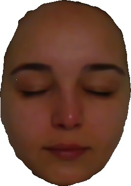
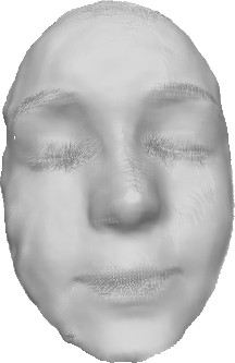
Face 3
Face 4
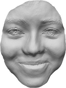
Face 5

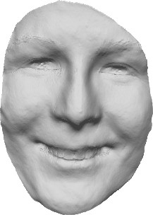
Figure 5: Results of the proposed variational approach to photometric depth super-resolution, using deep learning to estimate reflectance. Data was captured with an Intel Realsense D415 camera.

Next, we qualitatively evaluated our method on data we captured ourselves using an Intel RealSense D415 ($1280\times 720$ RGB and $640\times 360$ depth). The results in Figure 5 illustrate the ability of the proposed approach to recover detail-preserving geometry with subtle wrinkles and teeth details, in contrast with pure deep learning methods which are less accurate (see Section 4.3 in the supplementary material). Eventually, comparing the result on the “Face 1” dataset (Figure 1) against the shape-from-shading result from Section 3 also confirms the interest of replacing a model-based prior by a learning framework. However, the “Rucksack”’ and “Tabletcase” experiments of Figure 1 also highlight the limitation of the proposed learning-based solution: whenever the object significantly departs from usual facial appearance, the reflectance fails and artifacts arise in the depth map. This can also be observed on objects from the DiLiGenT dataset [41] (see Section 4.4 in the supplementary material), although our approach still outperforms other learning-based ones. The only way to circumvent such an issue is to acquire more data in a photometric stereo manner, as discussed in the next section.

5 Multi-Shot Depth Super-Resolution using Photometric Stereo

Single-shot depth super-resolution requires some prior knowledge of the surface reflectance, either in terms of a piecewise-constant prior or of adequation to a learning database. The only way to get rid of such priors consists in acquiring multiple observations under varying lighting, i.e. performing uncalibrated photometric stereo.

Let us consider from now on a sequence of images ${\{\mathbf{I}_{i}\}}$, $i\in\{1,\dots,n\}$ and $n\geq 4$, captured under varying lighting conditions denoted by ${\{\mathbf{l}_{i}\}}$. The image formation model (35) is then turned into the following system of $n$ equations:

$$\mathbf{I}_{i}=\mathbf{l}_{i}^{\top}\mathbf{m}_{z,\nabla z}\,{\bm{\rho}}+{\bm{\eta}_{\mathbf{I}}}_{i},\quad i\in\{1,\dots,n\}.$$ (21)

In (21), neither the depth $z$ nor the reflectance map ${\bm{\rho}}$ depends on $i$. Hence, their estimation is much more constrained in comparison with shape-from-shading. Nevertheless, nescience of the lighting vectors ${\{\mathbf{l}_{i}\}}$ makes the joint estimation of shape, reflectance and lighting an ill-posed problem: as discussed in Section 2, the arising ambiguities cannot be resolved without the introduction of additional priors. As we shall see now, in the context of RGB-D sensing the need for such priors can be circumvented and a purely data-driven approach can be followed. In other words, the low-resolution depth information act as a natural disambiguation prior for uncalibrated photometric stereo and, equally, the tailored photometric based-prior implicitly ensures surface regularity for depth map super-resolution.

5.1 Maximum Likelihood-Based Solution

Let us recall that the single-shot approach discussed in Section 3 required priors on the regularity of both the depth and the reflectance maps. By considering multiple RGB-D frames $\{\mathbf{I}_{i},z^{0}_{i}\}$, $i\in\{1,\dots,n\}$ of a static scene obtained under varying (though unknown) lighting, we hope to end up with a variational framework free of such man-made priors. To this end, we consider a maximum likelihood framework instead of a Bayesian one.

Considering again the independence of depth and image observations as well as the independence of shape from reflectance and lighting, the joint likelihood of the observations ${\{\mathbf{I}_{i},z^{0}_{i}\}}$ can be factored out as follows:

$$\mathcal{P}({\{\mathbf{I}_{i},z^{0}_{i}\}}|z,{\bm{\rho}},{\{\mathbf{l}_{i}\}})=\mathcal{P}({\{\mathbf{I}_{i}\}}|z,{\bm{\rho}},{\{\mathbf{l}_{i}\}})\,\mathcal{P}({\{z^{0}_{i}\}}|z).$$ (22)

Under the assumption that the random variables ${\bm{\eta}_{\mathbf{I}}}_{i}$ in (21) are homoskedastically distributed according to zero-mean Gaussian laws with the same covariance matrix $\text{diag}(\sigma_{I}^{2},\sigma_{I}^{2},\sigma_{I}^{2})$, the marginal likelihood for ${\{\mathbf{I}_{i}\}}$ can be explicitly written as

$$\mathcal{P}({\{\mathbf{I}_{i}\}}|z,{\bm{\rho}},{\{\mathbf{l}_{i}\}})\!\propto\!\exp\!\left\{\!-\frac{\sum_{i}\left\|\mathbf{l}_{i}^{\top}\!\mathbf{m}_{z,\nabla z}\,{\bm{\rho}}-\mathbf{I}_{i}\right\|_{2}^{2}}{2\sigma_{I}^{2}}\!\right\}.$$ (23)

Assuming that the $n$ low-resolution depth maps $z^{0}_{i}$ are consistent with the super-resolution model (32), and that the $n$ corresponding random variables ${\eta_{z}}_{i}$ follow a zero-mean Gaussian distribution with same variance $\sigma_{z}^{2}$, the marginal likelihood for ${\{z^{0}_{i}\}}$ writes as

$$\mathcal{P}({\{z^{0}_{i}\}}|z)\propto\exp\left\{-\frac{\sum_{i}\left\|Kz-z^{0}_{i}\right\|_{2}^{2}}{2\sigma_{z}^{2}}\right\}.$$ (24)

Maximum likelihood estimation of depth, reflectance and lighting consists in maximising the joint likelihood (22) or, equivalently, minimising its negative logarithm. Neglecting all additive constants and plugging (23) and (24) into (22), this writes as the following variational problem:

$$\min_{z,{\bm{\rho}},{\{\mathbf{l}_{i}\}}}\sum_{i}\left\|Kz-z^{0}_{i}\right\|_{2}^{2}+\gamma\left\|\mathbf{l}_{i}^{\top}\mathbf{m}_{z,\nabla z}\,{\bm{\rho}}-\mathbf{I}_{i}\right\|_{2}^{2},$$ (25)

with the trade-off parameter $\gamma$ given by the ratio $\gamma=\frac{\sigma_{z}^{2}}{\sigma_{I}^{2}}$. Let us emphasise the simplicity of the photometric stereo-based variational model (25), in comparison with the one obtained using shape-from-shading, cf. (10). Although one may think that more data introduces more complexity to such problems, we can clearly see here that in fact Problem (25) is naturally easier by itself as it does not include non-smooth prior terms on the albedo and the depth, but only two data terms. As discussed next, this allows a much simpler numerical strategy to be followed.

5.2 Numerical Solving of (25)

Contrarily to the shape-from-shading problem (10), in (25) the nonlinearity arises only from the unit-length constraint on the normals. Therefore, we opt for a simpler numerical solution based on fixed point iterations. Considering (33) and (35), (25) can be rewritten as

$$\min_{z,{\bm{\rho}},{\{\mathbf{l}_{i}\}}}\ \sum_{i}\left\|Kz-z^{0}_{i}\right\|_{2}^{2}+\gamma\left\|\mathbf{l}_{i}^{\top}\begin{bmatrix}\tilde{\mathbf{n}}_{z,\nabla z}/d_{z,\nabla z}\\ 1\end{bmatrix}{\bm{\rho}}-\mathbf{I}_{i}\right\|_{2}^{2},$$ (26)

with $\mathbf{n}_{z,\nabla z}=\tilde{\mathbf{n}}_{z,\nabla z}/d_{z,\nabla z}$, where $d_{z,\nabla z}$ is a scalar field ensuring the unit-length constraint of the normals:

$$d_{z,\nabla z}=\sqrt{\left|f\,\nabla z\right|^{2}+\left(-z-\mathbf{p}^{\top}\nabla z\right)^{2}},$$ (27)

and $\tilde{\mathbf{n}}_{z,\nabla z}$ is a vector field encoding the normal direction:

$$\tilde{\mathbf{n}}_{z,\nabla z}=\begin{bmatrix}f\,\nabla z\\ -z-\mathbf{p}^{\top}\nabla z\end{bmatrix}.$$ (28)

In (26), only $d_{z,\nabla z}$ depends in a nonlinear way on the unknown depth $z$. Therefore, it seems natural to solve (26) iteratively, while freezing the nonlinearity (contrarily to the shape-from-shading case, in photometric stereo we experimentally found this fixed point strategy to be convergent, though we leave the convergence proof for future work). At iteration $(k)$ and with the current estimates $({\bm{\rho}}^{(k)},\{\mathbf{l}_{i}^{(k)}\},z^{(k)})$, one sweep of this scheme reads:

$${\bm{\rho}}^{(k+1)}=\operatorname*{{argmin}}_{{\bm{\rho}}}\!\sum_{i}\!\left\|\mathbf{l}^{(k)\top}_{i}\!\!\begin{bmatrix}\tilde{\mathbf{n}}_{z^{(k)}\!,\nabla z^{(k)}}/d_{z^{(k)}\!,\nabla z^{(k)}}\\ 1\end{bmatrix}\!{\bm{\rho}}\!-\!\mathbf{I}_{i}\right\|_{2}^{2}\!,$$ (29)

$$\mathbf{l}^{(k+1)}_{i}=\operatorname*{{argmin}}_{\mathbf{l}_{i}}\left\|\mathbf{l}^{\top}_{i}\!\!\begin{bmatrix}\tilde{\mathbf{n}}_{z^{(k)}\!,\nabla z^{(k)}}/d_{z^{(k)}\!,\nabla z^{(k)}}\\ 1\end{bmatrix}\!{\bm{\rho}}^{(k+1)}-\mathbf{I}_{i}\right\|_{2}^{2}\forall i,$$ (30)

$$z^{(k+1)}=\operatorname*{{argmin}}_{z}\sum_{i}\left\|Kz-z^{0}_{i}\right\|_{2}^{2}$$ (31)

$$\qquad\qquad\qquad+\gamma\left\|\mathbf{l}^{(k+1)\top}_{i}\!\!\begin{bmatrix}\tilde{\mathbf{n}}_{z\!,\nabla z}/d_{z^{(k)}\!,\nabla z^{(k)}}\\ 1\end{bmatrix}\!{\bm{\rho}}^{(k+1)}-\mathbf{I}_{i}\right\|_{2}^{2}.$$

All three problems (29), (30) and (31) are linear least-squares problems which we solve using the conjugate gradient method on the normal equations.

Our initial values for $(k)=(0)$ are chosen to be ${\bm{\rho}}^{(0)}=\text{mean}({\{\mathbf{I}_{i}\}})$, $\mathbf{l}^{(0)}_{i}=[0,0,-1,0]^{\top}$ $\forall i$, and $z^{(0)}$ a smoothed version of $\text{mean}({\{z^{0}_{i}\}})$ using the guided filter [78] followed by bicubic interpolation to upsample to the image domain $\Omega_{HR}$. As in Section 3.2, to verify convergence we check if the relative residual $r_{\text{rel}}$ falls below some threshold. In our experiments convergence was reached within at most 15 iterations, which corresponds to a few minutes in our Matlab implementation.

5.3 Experiments

We first considered synthetic datasets in order to experimentally determine appropriate values for the hyper-parameter $\gamma$ and the number $n$ of images. The values $\gamma=0.01$ and $n\in[10,30]$ were found to represent an appropriate compromise between accuracy and runtime (see Section 5.2 in the supplementary material). We then carried out qualitative and quantitative comparisons of our results against state-of-the-art uncalibrated photometric stereo [37], shading-based depth refinement using a low-resolution RGB image [51] and image-driven depth super-resolution using an anisotropic Huber-loss as regularisation term [1, 91]. Our approach was found to be the most effective on both synthetic and publicly available real-world datasets [41]. These experiments can be found in Sections 5.3 to 5.5 in the supplementary material.

Then, we carried out a qualitative evaluation of our results on data we captured ourselves using an Asus Xtion Pro Live ($1280\times 1024$ RGB and $320\times 240$ depth) and an Intel Realsense D415 ($1280\times 720$ RGB and $640\times 480$ depth). The setup is the same as in Section 3.3, just multiple images of the same static scene with static camera under varying lighting conditions are captured. Varying lighting was created by freely moving a handheld LED light source during the capturing process. From each image sequence, $n=20$ high-resolution RGB images $\mathbf{I}_{i}$ and low-resolution depth images $z^{0}_{i}$ were randomly extracted. Results are displayed in Figure 6. “Face 2” results are even more satisfactory compared to the deep learning-based approach in Figure 5, despite a small spike on the nose due to a small specular spot being present in every input image. Even the fine wrinkles and the buttons of the “Shirt” are recovered. The thin structures of the “Backpack” are appropriately recovered and the partly very low reflectance does not seem to deteriorate the depth estimate. The “Oven mitt“ contains fine stitching structures which are successfully separated from the estimated albedo. The very fine geometric details of “Hat” are appropriately recovered in the depth, although some shading information remains visible in the reflectance. Interestingly, although our method is based on the Lambertian reflectance assumption, the high-quality shape of the reflective “Vase” can still be reconstructed and even where color is saturated at the specular regions, fine-scale geometric details are recovered. Eventually, among the three methods proposed in this article, only the uncalibrated photometric stereo-based approach can handle all three datasets in Figure 1, since reflectance is constrained neither to be piecewise-constant (“Rucksack”) nor to be that of a face (“Face 1”): the smoothly-varying albedo of the “Tabletcase” is appropriately estimated, and separated from the thin geometric wrinkle.

	one of $\mathbf{I}_{i}$	${\bm{\rho}}$	${z^{0}}$	$z$
Face 2
Shirt
Backpack
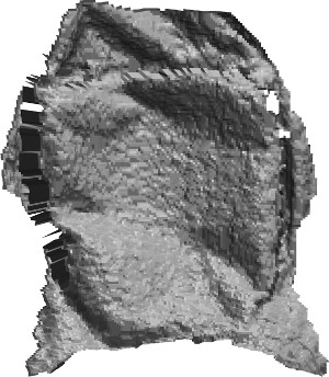
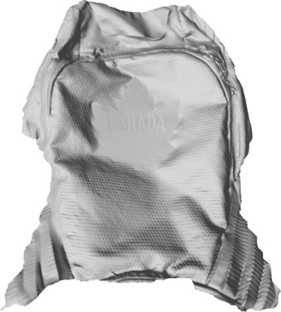
Oven mitt
Hat
Vase

Figure 6: Qualitative results of our uncalibrated photometric stereo-based method, on real-world data captured using a RealSense D415 (“Hat” and “Face 2”) or an Xtion Pro Live (five other datasets).

6 Conclusion

We investigated the use of photometric techniques for solving the depth super-resolution problem in RGB-D sensing. Three strategies were put forward: i) a shape-from-shading approach which requires a single RGB-D frame but is limited to objects exhibiting piecewise-constant reflectance, ii) a reflectance learning one which loosens this assumption by delegating reflectance estimation to a deep neural network trained on a specific class of objects such as faces, and iii) an uncalibrated photometric stereo setup which bypasses the need for albedo prior or training by acquiring additional data. These three approaches represent a continuum of solutions to photometric depth super-resolution with increasing level of accuracy, yet increasing amount of required resources.

This work may still be completed in several manners. First, the theoretical properties (proofs of convergence, existence and uniqueness of solutions, etc.) of the proposed numerical schemes may be explored. Second, all the methods presented here explicitly use the linear Lambertian image formation model: a natural line of future research would be to improve robustness to off-Lambertian effects such as specularities and cast-shadows, by resorting either to robust estimation techniques as in [42], or to non-Lambertian image formation models as in [92]. Eventually, the combination of deep learning and variational techniques might be further explored, for instance by devoting not only reflectance estimation to a deep neural network, but also lighting estimation as in [93]. Put together, these novelties could allow our approaches to handle more general surfaces as well as more general illumination conditions.

Appendix A Organization of the document

This document is structured as follows. Section B contains general comments on photometric 3D-reconstruction and depth super-resolution: the derivation of the RGB image formation model used through the paper, a visual description of the ambiguities arising in depth super-resolution and in shape-from-shading, and some general information regarding the reflectance learning-based approach. The rest of the document is devoted to the individual experimental evaluation of each of the proposed methods: Section C contains the shape-from-shading experiments, Section D the reflectance learning ones, and Section E evaluates the uncalibrated photometric stereo-based approach. Section F eventually concludes the document by presenting a unified comparison of the results obtained with the three proposed methods.

Appendix B Generalities

B.1 Derivation of the RGB image formation model

This subsection is devoted to the derivation of the RGB image formation model (Eq. (3) in the main paper), which relates the irradiance measurements and the surface normals. The following derivation is adapted from [94, Sect. 2.2], with an extension of the model to RGB images and spherical harmonics lighting.

We first assume that the surface is Lambertian, i.e. its appearance is independent from the viewing angle. A consequence of this assumption is that the surface’s reflectance $\rho$ at a surface point is a simple scalar quantity called the albedo, which is independent from the incident light direction.

Next, we assume that the surface is lit by a single, infinitely distant light source represented by a direction $\omega$ on the visible hemisphere. The spectral radiance at a surface point is thus given by

$$L(\lambda,\omega)=\phi(\lambda,\omega)\,\dfrac{\rho(\lambda)}{\pi}\,\max\{0,\mathbf{s}(\omega)^{\top}\mathbf{n}_{z,\nabla z}\},$$ (32)

with $\lambda$ the wavelength, $\phi(\cdot,\omega)$ the spectrum of the source associated with direction $\omega$, $\rho(\cdot)$ the spectral reflectance of the surface point, $\mathbf{s}(\omega)$ the unit-length vector pointing towards the light source associated with direction $\omega$, and $\mathbf{n}_{z,\nabla z}$ the outer unit-length surface normal.

Now, let us assume that the surface is observed under natural illumination, rather than lit by one single light source. Let us represent natural illumination by a collection of infinitely distant point light sources, each of them being represented by a direction $\omega$. The total spectral radiance of a surface point is obtained by summing the individual contributions from each source, i.e. by integrating (32) over the visible hemisphere:

$$L(\lambda)=\dfrac{\rho(\lambda)}{\pi}\int_{\mathbb{S}^{2}}\phi(\lambda,\omega)\,\max\{0,\mathbf{s}(\omega)^{\top}\mathbf{n}_{z,\nabla z}\}\,\mathrm{d}\omega.$$ (33)

We further assume that the sensor’s response is linear, and that the RGB camera is focused on the surface. Then, the sensor’s spectral irradiance, in the pixel conjugate to the surface point, is given by

$$E(\lambda)=\beta\cos^{4}\alpha\,L(\lambda),$$ (34)

where $\beta$ depends on the sensor’s aperture and magnification, and where $\alpha$ is the angle between the viewing angle and the optical axis (the $\cos^{4}\alpha$ factor is thus responsible for darkening at the periphery of images).

The intensity recorded by the camera in channel $\star$, $\star\in\{R,G,B\}$, is proportional to the sum of all spectral sensor’s irradiances, weighted by the camera’s transmission spectrum. Denoting by $\gamma$ this proportionality coefficient, this writes as

$$I_{\star}=\gamma\int_{\mathbb{R}^{+}}c_{\star}(\lambda)E(\lambda)\,\mathrm{d}\lambda,$$ (35)

with $c_{\star}(\lambda)$ the transmission spectrum of camera’s channel $\star$.

We further assume that all the light sources are achromatic, i.e. that

$$\phi(\lambda,\omega)=\phi(\omega)$$ (36)

(this assumption implies that color will be interpreted in terms of surface’s reflectance by our algorithms, rather than in terms of lighting).

Plugging Equations (33), (34) and (36) into (35) yields

$$I_{\star}=\rho_{\star}\int_{\mathbb{S}^{2}}\phi(\omega)\max\{0,\mathbf{s}(\omega)^{\top}\mathbf{n}_{z,\nabla z}\}\,\mathrm{d}\omega,$$ (37)

with

$$\rho_{\star}:=\dfrac{\gamma\beta\cos^{4}\alpha}{\pi}\int_{\mathbb{R}^{+}}c_{\star}(\lambda)\rho(\lambda)\,\mathrm{d}\lambda$$ (38)

the “albedo”, relatively to channel $\star$ (note that $\rho_{\star}$ does not characterize the surface, since it depends upon the sensor’s response, its aperture and magnification, etc.).

Next, we approximate the integral in (37) using spherical harmonics [4, 5]. In this work we consider the first-order case, which already captures more than $85\%$ of natural illumination [95], and leave the extension to second-order spherical harmonics as future work. The spherical harmonics approximation reads

$$\int_{\mathbb{S}^{2}}\ \phi(\omega)\max\{0,\mathbf{s}(\omega)^{\top}\mathbf{n}_{z,\nabla z}\}\,\mathrm{d}\omega\approx\mathbf{l}^{\top}\mathbf{m}_{z,\nabla z}$$ (39)

with $\mathbf{l}\in\mathbb{R}^{4}$ the achromatic “light vector” (which is the same for all pixels), and

$$\mathbf{m}_{z,\nabla z}:=\begin{bmatrix}\mathbf{n}_{z,\nabla z}\\ 1\end{bmatrix}$$ (40)

a geometric vector depending upon the surface normals.

Plugging (39) into (37), we obtain

$$I_{\star}=\rho_{\star}\,\mathbf{l}^{\top}\mathbf{m}_{z,\nabla z},\quad\star\in\{R,G,B\}.$$ (41)

Denoting

$$\mathbf{I}:=\begin{bmatrix}I_{R}\\ I_{G}\\ I_{B}\end{bmatrix}\quad\text{and}\quad{\bm{\rho}}:=\begin{bmatrix}\rho_{R}\\ \rho_{G}\\ \rho_{B}\end{bmatrix},$$ (42)

and assuming that (41) is satisfied up to additive noise, we eventually obtain the RGB image formation model (Eq. (3) in the paper) by plugging together the three equations in (41):

$$\mathbf{I}=\mathbf{l}^{\top}\mathbf{m}_{z,\nabla z}\,{\bm{\rho}}+{\bm{\eta}_{\mathbf{I}}},$$ (43)

with ${\bm{\eta}_{\mathbf{I}}}$ the realisation of a stochastic process.

B.2 Ambiguities in Depth Super-resolution and Shape-from-shading

This subsection illustrates the ambiguities arising in depth super-resolution and in photometric 3D-reconstruction, in order to visually motivate the choice of their joint solving. As can be seen in Figure 7, in super-resolution high-frequency geometric clues are missing and thus there exist infinitely many ways to interpolate between low-resolution samples. On the contrary, shape-from-shading suffers from the concave $/$ convex ambiguity: though the surface orientation is unambiguous in critical points (arrows in Figure 8), two such singular points may be connected either by “going up” or by “going down”. Therefore, it seems reasonable to rely on high-frequency photometric clues to disambiguate depth super-resolution, and on low-frequency geometric clues to disambiguate photometric 3D-reconstruction.

Figure 7: There exist infinitely many ways (dashed lines) to interpolate between low-resolution depth samples (rectangles). Our disambiguation strategy builds upon shape-from-shading applied to the companion high-resolution color image (cf. Figure 8), in order to resurrect the fine-scale geometric details of the genuine surface (solid line).

Figure 8: Shape-from-shading suffers from the concave $/$ convex ambiguity: the genuine surface (solid line) and both the surfaces depicted by dashed lines produce the same image, if lit and viewed from above. We put forward low-resolution depth clues (cf. Figure 7) for disambiguation.

B.3 Generalities on Reflectance Learning-based Depth Super-resolution

We now illustrate the creation of the training dataset and the network’s architecture, and justify why we focused on a particular class of objects in the learning-based approach.

Figure 9 illustrates the generation of training data. We consider ground truth geometry and reflectance of various human faces from the ICT-3DRFE database [89]. A rendering software is used to generate multiple images of these faces under different viewing and lighting scenarios. Lighting variations are created by turning off and on several extended sources, emulating usual indoor lighting conditions.

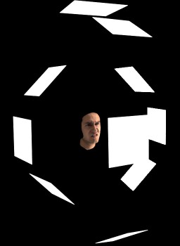
Figure 9: Rendering of synthetic faces for generating training data. The white planes represent switchable extended light sources, which are independently controlled to create multiple illumination conditions. Multiple images can then be captured under different illumination and viewing angles.

Figure 10 illustrates the architecture of the neural network. It is a U-Net architecture comprising an initial convolution layer of kernel size 4, stride 2 and padding 1; after which there are repeated blocks of 8 ReLU-Conv-BatchNorm layers. This results in downsampling of a 512x512 resolution image to a 1x512 vector at the bottleneck of the “U”. Then, the 1D array is upsampled to input resolution with multiple ReLU-Transpose Convolution-BatchNorm layers. Dropout is also used in a few layers to allow for randomness while learning the mapping from input images to albedo maps. Finally, the L1 loss is considered, which favors sharper output compared to the L2 loss.

Figure 10: The U-Net Architecture used for albedo estimation. The top two layers are the input and output, respectively. The arrows’ color represent the operations of the other hidden layers. Skip connections (dotted lines) concatenate the left and right layers.

Eventually, Figure 11 illustrates the lack of inter-class generalisation which is inherent to learning-based methods. For instance, the approach of [96] (trained on Sintel [97] and MIT [98] datasets) performs well on the MIT object but poorly on the ShapeNet car image, because such an object was not present in the learning database. For the same reason, the alternative approach of [87] (trained on ShapeNet objects [99]) performs well on the ShapeNet car but fails on the MIT object, and both approaches fail on the face image since the latter resembles none of the training data. Due to this lack of inter-class generalisation, we choose to focus in our approach on the specific class of human faces.

Input Image	[96]	[87]

Figure 11: Learning-based albedo estimation applied to an object from the MIT database (first row), a car from the ShapeNet dataset (second row), and two images of human faces we generated with a renderer using the ICT-3DRFE database [89]. This illustrates the lack of inter-class generalisation inherent to learning-based techniques: the approach from [96], trained on the MIT dataset, fails on the ShapeNet car and on faces, and the one from [87], trained on the ShapeNet dataset, fails on the MIT object and on faces: in both cases albedo estimation is not satisfactory since the objects do not resemble the training data.

	Lucy[100]	Thai Statue[100]	Armadillo[100]	Joyful Yell[101]
$\mathbf{I}$
	“voronoi” albedo	“voronoi” albedo	“rectcircle” albedo	“bar” albedo
${z^{0}}$

Figure 12: Illustration of synthetic data used for evaluation of the single-shot approach based on shape-from-shading. High-resolution RGB images $\mathbf{I}$, of size $480\times 640$, are generated using high-resolution ground truth depth and reflectance maps, and adding noise. Low-resolution depth maps ${z^{0}}$ are created by downsampling the ground truth depth maps with scaling factors of $8$, $4$ and $2$ (the second row shows the low-resolution depth maps with a scaling factor of $2$), and adding noise.

Appendix C Evaluation of the Single-shot Approach based on Shape-from-shading

C.1 Creation of the Synthetic Data

Figure 12 illustrates the synthetic data used for evaluation, which is generated using four different 3D-shapes (“Lucy”, “Thai Statue”, “Armadillo” and “Joyful Yell”), each of them rendered using three different albedo maps (“voronoi”, “rectcircle” and “bar”) and three different scaling factors (2, 4 and 8) for the low-resolution depth image. To this end, 3D-meshes are rendered into high-resolution ground truth depth maps of size $480\times 640$, which are then downsampled. Then, additive zero-mean Gaussian noise with standard deviation $10^{-4}$ times the squared original depth value (consistently with real-world measurements from [102]) is added to the low-resolution depth maps, which are eventually quantised. High-resolution RGB images are rendered from the ground truth depth map using the first-order spherical harmonics model with $\mathbf{l}=[0,0,-1,0.2]^{\top}$ using the three different high-resolution reflectance maps, and an additive zero-mean Gaussian noise with standard deviation $1\%$ the maximum intensity is eventually added to the RGB images.

C.2 Tuning the Hyper-parameters

In Figure 13, we use the “Joyful Yell” dataset from Figure 12 in order to determine appropriate values for the hyper-parameters $(\mu,\nu,\lambda)$. For quantitative evaluation, we consider the root mean squared error (RMSE) on the estimated depth and reflectance maps, and the mean angular error (MAE) on surface normals. To select an appropriate set of values for them, we initially set $\mu=0.5$, $\nu=0.01$ and $\lambda=1$. We then evaluate the impact of each parameter by varying it while keeping the remaining two fixed. As could be expected, large values of $\mu$ force the depth map to keep close to the noisy input, while small values make the depth prior less important so not capable of disambiguating shape-from-shading. Inbetween, the range $\mu\in[10^{-1},10]$ seems to provide appropriate results. As for $\nu$, large values produce over-smoothed results and small ones result in slightly noisier depth estimates, although the albedo estimate seems unaffected by this choice. Overall, the range $\nu\in[0.5,10^{2}]$ seems appropriate. The parameter $\lambda$ strongly impacts both the resulting albedo and depth: too small (resp., high) values for $\lambda$ result in over (resp., under)-segmentation problems, and in both cases shading information gets propagated to the albedo. We found $\lambda\in[10^{-1},10]$ to be a reasonable choice. Overall, we opted for $(\mu,\nu,\lambda)=(0.1,0.7,1)$.

	$\mu$	$\nu$	$\lambda$
RMSE (depth)
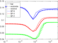
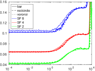
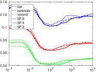
MAE (depth)
RMSE (albedo)

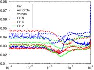
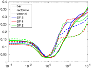
Figure 13: Impact of the parameters $(\mu,\nu,\lambda)$ on the accuracy of the albedo and depth estimates. The accuracy of the albedo is evaluated by the root mean square error (RMSE), and that of the depth by the RMSE and the mean angular error (MAE). Based on these experiments, the set of hyper-parameters $(\mu,\nu,\lambda)=(0.1,0.7,1)$ is selected.

C.3 Comparison against the State-of-the-art on the Synthetic Dataset

Next, we compare the results obtained by our single-shot approach against the state-of-the-art, on the synthetic dataset from Figure 12. We consider two alternative depth super-resolution methods: the image-based one from [60], and the learning-based one from [10] (since the authors only provide trained data for a factor of $4$, this method was evaluated only for this factor). To emphasise the interest of joint shape-from-shading and depth super-resolution over shading-based depth refinement using downsampled images, we also consider [51]. Qualitative results are presented in Figure 14, and quantitative ones in Table I. As can be seen, our method systematically overcomes the competitors in terms of MAE, which indicates that high-frequency geometric details are better recovered. The RMSE on depth rather evaluates the overall (low-frequency) fit to ground truth, and for this metric our results are comparable with [60], which achieves the best results.

Interestingly, for scaling factors of $4$ and $8$, our approach seems less accurate than [60] in terms of RMSE. However, Figure 14 clearly shows that our results are significantly better: we thus believe that only the order of magnitude of the RMSE is meaningful, yet comparison using this metric might not really indicate which method is the best, and MAE should be preferred for this purpose. A more thorough discussion on the relevance of RMSE for evaluation can be found in [103].

	Lucy “voronoi”	Thai Statue “voronoi”	Armadillo “rectcircle”	Joyful Yell “bar”
[60]
[10]
[51]
Ours

Figure 14: Qualitative comparison between our single-shot results and state-of-the-art’s ones (the scaling factor is $4$).

Albedo	3D-shape	SF	[60]		[10]		[51]		Ours
			RMSE	MAE	RMSE	MAE	RMSE	MAE	RMSE	MAE
bar		2	0.043643	38.6274	–	–	0.41993	67.2643	0.034655	16.7496
	Armadillo	4	0.051558	42.2277	0.17865	45.6972	0.45139	66.2117	0.054679	19.0314
		8	0.072466	43.5649	–	–	0.58837	69.3262	0.091263	20.8836
		2	0.05089	29.1719	–	–	0.1721	47.4836	0.050694	16.7414
	Joyful Yell	4	0.066517	33.0843	0.084094	42.611	0.22867	32.9784	0.079271	19.0695
		8	0.10212	36.565	–	–	0.37923	31.2894	0.128	21.9886
		2	0.057987	39.4714	–	–	0.21309	66.5525	0.053989	25.0955
	Lucy	4	0.068502	42.7169	0.50472	47.605	0.34091	69.2566	0.081005	28.3044
		8	0.098713	46.4775	–	–	0.43619	59.5434	0.1195	30.1058
		2	0.040821	42.8976	–	–	0.12948	63.06	0.035736	23.9147
	Thai Statue	4	0.050296	47.1017	0.22363	49.9553	0.15489	54.6139	0.057313	28.492
		8	0.066515	49.8604	–	–	0.22835	56.4247	0.087054	31.65
rectcircle		2	0.044026	39.108	–	–	0.34323	70.8526	0.03494	18.4909
	Armadillo	4	0.052115	43.3175	0.17782	45.6324	0.2338	50.6919	0.056727	18.8487
		8	0.069467	45.4735	–	–	0.61917	70.9363	0.09155	21.9959
		2	0.051296	30.7886	–	–	0.14841	41.5424	0.05226	17.134
	Joyful Yell	4	0.066911	33.3	0.10328	42.7531	0.28311	51.0665	0.080387	19.8717
		8	0.10201	36.2961	–	–	0.39518	35.4817	0.1281	22.8027
		2	0.058495	39.7374	–	–	0.19546	64.8212	0.054383	24.8427
	Lucy	4	0.069893	43.9016	0.50464	48.1068	0.23235	53.2901	0.082547	28.7517
		8	0.099402	46.3739	–	–	0.39583	64.3269	0.12283	29.1531
		2	0.039821	40.6144	–	–	0.11355	58.2254	0.036845	23.9036
	Thai Statue	4	0.04973	46.1154	0.20894	49.4124	0.16749	52.9663	0.05866	28.155
		8	0.067799	50.6515	–	–	0.21058	50.9074	0.094688	33.5308
voronoi		2	0.043635	38.9089	–	–	0.33005	69.3157	0.034751	17.6873
	Armadillo	4	0.051989	41.57	0.17182	45.5833	0.4407	65.5811	0.056032	20.168
		8	0.07077	43.1987	–	–	0.50548	63.8618	0.090708	22.2767
		2	0.052002	28.7903	–	–	0.16893	47.72	0.052429	17.0453
	Joyful Yell	4	0.066557	32.3448	0.086394	43.1744	0.24753	39.6569	0.079888	19.6512
		8	0.10238	35.8017	–	–	0.47694	47.4707	0.12916	21.6663
		2	0.058222	36.2327	–	–	0.29164	72.9002	0.054442	26.1333
	Lucy	4	0.068253	40.8878	0.5066	48.0387	0.32955	71.1042	0.079877	28.4506
		8	0.099838	43.7671	–	–	0.37839	57.6856	0.11877	29.6331
		2	0.039872	39.6508	–	–	0.13261	65.8352	0.037607	25.6126
	Thai Statue	4	0.049783	45.7178	0.22688	49.4132	0.16533	58.3933	0.058957	28.6314
		8	0.065577	48.7962	–	–	0.21927	49.6711	0.091959	32.0347
		2	0.047458	39.0085	–	–	0.18378	65.3282	0.044151	21.1973
Median		4	0.059316	42.4723	0.19379	46.6511	0.24067	53.952	0.069114	24.1615
		8	0.085589	44.6203	–	–	0.3955	57.0551	0.10673	25.9779
		2	0.048392	36.9999	–	–	0.22154	61.2978	0.044394	21.1126
Mean		4	0.059342	41.0238	0.24812	46.4986	0.27298	55.4842	0.068779	23.9521
		8	0.084754	43.9022	–	–	0.40275	54.7438	0.1078	26.4768

TABLE I: Quantitative comparison between our single-shot results and three state-of-the-art methods, on all the synthetic datasets. Our results are always superior in terms of mean angular error (MAE) and in terms of root mean square error (RMSE) when the scaling factor is $2$. For larger synthetic factors our RMSE values are slightly higher than those from [60], but Figure 14 shows that our results are actually of better quality than the latter, so the RMSE values might not be as relevant as the MAE ones.

C.4 Comparison against the State-of-the-art on a Public Real-world Dataset

In Figure 15, we qualitatively compare our single-shot results against the state-of-the-art, using the real-world DiLiGenT photometric stereo dataset [41] (only one out the 96 images of each object was used). To create noisy low-resolution input depths with a scaling factor of $2$, $4$ and $8$, the ground truth depth is downsampled and Gaussian noise is then added, as in the previous subsection.

On objects which match our assumption of a Lambertian surface with piecewise-constant albedo (e.g., “bear” and “pot1”), we obtain very satisfactory results. However, the strong dependency of our approach on the piecewise-constant albedo assumption is clearly visible in the “cat” results, which are not as satisfactory: the dark structures in the image are too thin to be appropriately interpreted as piecewise-constant albedo areas and this creates artifacts in the geometry.

Besides, the “cow”, “pot2” and “reading” results demonstrate that our approach also strongly depends upon the Lambertian assumption: the specular highlights in the images get propagated into the estimated depth. A natural future extension of our method would thus be to cope with such non-Lambertian effects, either by resorting to robust estimation techniques [42], or by adapting our approach to a non-Lambertian image formation model[92].

Nevertheless, and despite these important limitations, our results remain qualitatively superior to those of the state-of-the-art in all the experiments. This can also be observed in the quantitative evaluation of Table II, which confirms the conclusions of the synthetic quantitative evaluation from Table I.

	$\mathbf{I}$	${z^{0}}$	[60]	[10]	[51]	Ours	Ground truth
bear
buddha
cat
cow
goblet
harvest
pot1
pot2
reading

Figure 15: Qualitative comparison between our single-shot results and those from the state-of-the-art, on the DiLiGenT dataset [41] (the scaling factor is 4). Our approach outperforms the state-of-the-art in all the experiments.

3D-shape	SF	[60]		[10]		[51]		Ours
		RMSE	MAE	RMSE	MAE	RMSE	MAE	RMSE	MAE
	2	0.0066575	17.2655	–	–	0.014616	27.9357	0.0047136	12.8781
bear	4	0.0065535	19.5072	0.8825	31.5392	0.028849	31.8918	0.0085904	14.8113
	8	0.97126	76.4581	–	–	0.055159	31.0276	0.018022	20.341
	2	0.0099968	37.3338	–	–	0.02972	69.0274	0.0080152	26.6017
buddha	4	0.0099935	39.1319	0.86352	36.8237	0.038584	68.6713	0.012027	31.0774
	8	1.3683	71.2403	–	–	0.047353	57.6881	0.019676	39.0075
	2	0.0085294	23.3362	–	–	0.028382	44.6708	0.0084811	18.8204
cat	4	0.0096136	27.826	0.80869	30.7428	0.042872	54.1746	0.01353	21.4786
	8	0.015137	30.8242	–	–	0.065853	53.4602	0.023393	25.3616
	2	0.0086552	32.7633	–	–	0.037772	59.2638	0.0049385	14.806
cow	4	0.0090334	33.8093	0.84557	33.7576	0.055621	55.3108	0.0089681	16.9767
	8	0.010392	31.6684	–	–	0.059261	53.5979	0.017596	21.03
	2	0.01019	30.2473	–	–	0.032588	59.1553	0.011007	23.0414
goblet	4	0.011121	31.1036	1.3435	34.0517	0.048727	56.7471	0.017208	24.2692
	8	0.015451	36.2801	–	–	0.084675	51.7091	0.031125	25.7217
	2	0.014169	33.9026	–	–	0.041792	66.3635	0.01594	31.1557
harvest	4	2.651	63.9349	0.75973	37.0383	0.05696	66.5893	0.023588	33.6957
	8	115.5837	79.2204	–	–	0.074651	50.9501	0.037176	35.9762
	2	0.0077563	22.6961	–	–	0.020767	48.3748	0.007147	16.9523
pot1	4	0.0086358	26.2298	0.72979	31.8426	0.03114	39.7103	0.010863	17.6975
	8	0.013278	29.6214	–	–	0.05537	38.9525	0.019307	19.9866
	2	0.0081729	28.8295	–	–	0.021455	50.4214	0.0055283	18.0749
pot2	4	0.0088839	32.7579	0.90388	33.4448	0.028528	28.5455	0.0088442	19.2421
	8	0.014079	35.288	–	–	0.054661	47.9005	0.01623	22.4169
	2	0.011767	28.7648	–	–	0.030566	53.4663	0.0097283	19.2611
reading	4	0.011428	30.4347	0.93384	31.764	0.047677	53.7065	0.015536	22.91
	8	0.01607	32.2913	–	–	0.071794	52.5448	0.028808	29.0107
	2	0.0086552	28.8295	–	–	0.02972	53.4663	0.0080152	18.8204
Median	4	0.0096136	31.1036	0.86352	33.4448	0.042872	54.1746	0.012027	21.4786
	8	0.015451	35.288	–	–	0.059261	51.7091	0.019676	25.3616
	2	0.0095439	28.3488	–	–	0.028629	53.1865	0.0083887	20.1769
Mean	4	0.30292	33.8595	0.89678	33.4449	0.042106	50.5941	0.013239	22.4621
	8	13.112	46.988	–	–	0.063197	48.6479	0.023481	26.5391

TABLE II: Quantitative comparison between our single-shot results and those from the state-of-the-art, on the DiliGenT dataset [41]. Our approach systematically outperforms the state-of-the-art, consistently with the conclusions from the synthetic experiments drawn in Table I.

C.5 Comparison against State-of-the-art Multi-view Techniques on Publicly Available Real-world Datasets

Figure 16 shows four qualitative comparisons with state-of-the-art multi-view approaches on publicly available datasets. The “Augustus”, “Lucy” and “Relief” datasets [47] were created using a PrimeSense camera, whereas “Gate” [104] was acquired using a Structure Sensor for the iPad. The scaling factor for “Augustus”, “Relief” and “Gate” is $2$, whereas it is $1$ for “Lucy” (in this case, our approach only performs shading-based depth refinement without super-resolution). Although our approach needs significantly less data (a single RGB-D image) compared to multi-view approaches, we are still able to recover fine geometry close to the degree of detail of [47, 46]. Even under more complex lighting, as for instance in the “Gate” experiment, our approach can result in high-resolution depth maps with fine-scale details.

	$\mathbf{I}$	${\bm{\rho}}$	${z^{0}}$	[47]/[46]	Ours
Augustus
Lucy
Relief
Gate

Figure 16: Qualitative comparison against state-of-the-art multi-view approaches. Although it uses a single RGB-D frame, our approach results in depth maps whose quality is comparable with those obtained using multi-view data.

C.6 Additional Comparison against State-of-the-art Single-shot Techniques on Real-world Datasets we Captured Ourselves

Figure 17 shows additional qualitative comparison of single-shot results, on data we captured using an Asus Xtion Pro Live camera (scaling factor of $4$). Once again, our approach outperforms the state-of-the-art, even though under- or over-segmentation of the reflectance may happen.

	$\mathbf{I}$	${\bm{\rho}}$	${z^{0}}$	[60]	[10]	[51]	Ours
Blanket
Clothes
Failure
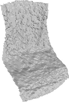
Monkey
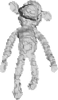
Wool

Figure 17: Qualitative comparison of state-of-the-art single-view approaches on five real-world datasets captured with an Asus Xtion Pro Live camera at resolution $1280\times 960$ for the RGB images and $320\times 240$ for the low-resolution depth.

The “Clothes” experiment illustrates a case where over-segmentation of reflectance happens, but interestingly this does not seem to impact depth recovery. Whenever color gets saturated (some of the balls of “Wool”) or too low (black areas in the “Blanket”), then minimal surface drives super-resolution: the areas where brightness is not informative are simply smoothed out, which adds robustness. Our method only fails when reflectance does not fit the Potts prior, as shown in the “Failure” experiment. In this case of an object with smoothly-varying reflectance, under-segmentation of reflectance happens, and all the thin brightness variations are interpreted in terms of geometry. Two alternative strategies are investigated in this work to cope with this issue: estimate reflectance without a piecewise-constant prior (learning-based strategy), or actively control lighting (photometric stereo-based strategy).

	${z^{0}}$	[60]	[10]	[51]	Ours	1D depth profiles
Android
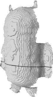
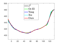
Basecap
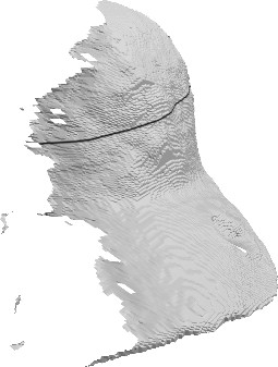
Minion
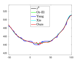
Rucksack

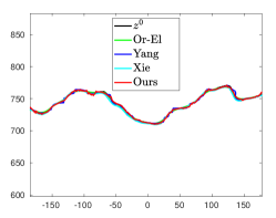
Figure 18: Qualitative comparison between our single-shot results and those from the state-of-the-art, on the datasets from Figure 3 in the main paper. Our approach systematically outperforms the state-of-the-art. The rightest column shows 1D depth profiles corresponding to the lines drawn on the 3D-shapes: although the depth estimated using all the methods overall fit well together, ours is the only which provides reasonable fine-scale details.

Eventually, Figure 18 presents another qualitative comparison on the real-world data from Figure 3 in the main paper (captured using a RealSense D415 camera). Note that [60] seems to give good depth estimates whenever the underlying assumption (an edge in the RGB image coincides with an edge in the depth image) is met, cf. “Rucksack” experiment, but it fails to provide detail-preserving depth maps when reflectance is uniform or changes only slightly (“Android” and “Minion” experiments), since it uses only a sparse set of information from the RGB data. Unsurprisingly, the method from [10] cannot hallucinate surface details, since it does not use the color image. The shading-based depth refinement method of [51] does a much better job at improving geometry, but it is largely overcome by the proposed shading-based depth super-resolution approach, because the latter uses information from a higher-resolution RGB image.

Appendix D Evaluation of the Reflectance Learning-based Approach

D.1 Creation of the Synthetic Data

Let us first recall that the reflectance learning-based approach was trained on data extracted from the ICT-3DRFE Database [89]. In order to evaluate this approach, we considered two subjects from this database as well, each one enacting $10$ different facial expressions. Of course, in order to avoid any bias, these subjects were not used when training the neural network.

The high-resolution RGB and low-resolution depth images were created in a similar manner as in the previous section: high-resolution RGB images of the faces were rendered at $512\times 512$ resolution from the ground truth albedo and depth under first-order spherical harmonics lighting $\mathbf{l}=[0,0,-1,0.2]^{\top}$; and the low-resolution depth maps were created by downsampling the ground truth depth by a scaling factor of $2$, $4$ and $8$. Zero-mean Gaussian noise with standard deviation $1\%$ the maximum RGB intensity was then added to the RGB images, and zero-mean Gaussian noise with standard deviation $10^{-4}$ the squared original depth value (consistently with the real-world measurements from [102]) was added to the low-resolution depth maps, before quantisation.

These synthetic faces were then used for quantitative evaluation of the proposed reflectance learning-based approach against the state-of-the-art and against the proposed fully variational solution, as discussed in the next subsection.

D.2 Comparison against the State-of-the-art on the Synthetic Dataset

We next evaluate our method, which first estimates reflectance using deep learning and then achieves variational depth super-resolution using the RGB image, in comparison with end-to-end deep learning solutions for geometry estimation.

For comparison, we first consider the method introduced in [62], which is an end-to-end depth super-resolution technique based on low-resolution depth data and high-resolution RGB image, i.e. the same inputs as our methods. It can be seen in Figure 19 that this end-to-end solution fails to recover surface details which are visible in the RGB image.

In order to evaluate the ability of deep networks to reconstruct geometry from a single RGB image, similarly to shape-from-shading techniques, we also show the results of SfSNet [86], which is a deep learning-based method estimating albedo and surface normals (which we further integrated into a depth map using the quadratic integation method discussed in [105]) out of a single RGB image. SfSNet is limited to RGB images of size $128\times 128$, so it was evaluated only for a scaling factor of $4$ and, since it does not perform depth super-resolution, the ground truth depth was downsampled for the quantitative evaluation of this method. Figure 19 shows that reasonable results can be expected using SfSNet, yet geometry is slightly oversmoothed in comparison with what can be obtained using the proposed combination of machine learning and variational approaches.

Eventually, we compare this combined approach with the fully variational one from the previous section. The latter does not completely fail at recovering a reasonable geometry, but since the estimated albedo is piecewise-constant and departs significantly from the ground truth, artifacts and noise are propagated to the estimated geometry. This is confirmed by the quantitative evaluation in Table III, which clearly indicates that the proposed combination of machine learning and variational methods is more efficient than both end-to-end learning solutions from the state-of-the-art and the proposed fully variational approach.

	$\mathbf{I}$	${z^{0}}$	[62]	[86]	Ours (SfS)	Ours	Ground truth [89]
S4E4
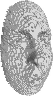
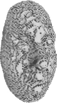
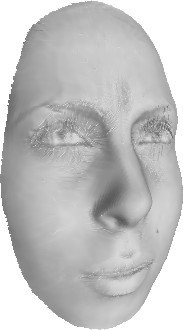
S4E9
S11E5
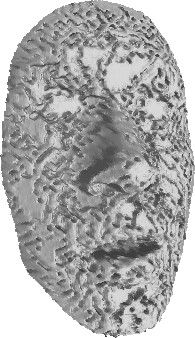
S11E6

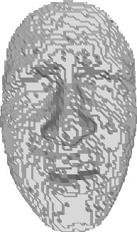
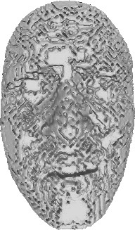
Figure 19: Qualitative comparison of the results obtained using the deep learning-based depth super-resolution technique from [62], the deep learning-based shape-from-shading approach from [86], the proposed variational approach to shape-from-shading (denoted by SfS), and the proposed combination of deep learning and variational methods. The latter seems the most effective, and this is confirmed by the quantitative evaluation provided in Table III.  
 

Subject (S)	Expression (E)	SF	[62]		[86]		Ours (SfS)		Ours
			RMSE	MAE	RMSE	MAE	RMSE	MAE	RMSE	MAE
4		2	0.1572	48.3553	–	–	0.1613	14.1551	0.1355	9.9354
	0	4	0.13284	36.9774	0.6071	13.4647	0.10629	11.6301	0.086867	8.5443
		8	0.63	38.0244	–	–	0.24354	14.2278	0.19869	11.0617
		2	0.15451	48.4316	–	–	0.15824	15.2649	0.13413	10.6932
	1	4	0.13069	36.4169	0.7185	14.3254	0.10972	12.8361	0.087058	9.5301
		8	0.61295	35.7076	–	–	0.25859	15.2818	0.20735	12.0648
		2	0.15358	49.0454	–	–	0.14589	14.516	0.14005	14.221
	2	4	0.13266	37.1973	0.8821	18.5108	0.12322	13.9566	0.10993	13.2265
		8	0.97825	38.8272	–	–	0.27613	17.4243	0.25379	16.0565
		2	0.15657	48.4417	–	–	0.1614	14.776	0.14468	11.1379
	3	4	0.13335	37.0725	0.8554	16.0271	0.11759	13.165	0.09558	10.604
		8	0.95333	38.6755	–	–	0.26179	15.8035	0.21567	13.0665
		2	0.15155	48.3665	–	–	0.14914	14.5008	0.13132	11.1096
	4	4	0.13093	37.2093	0.6301	15.0882	0.1108	12.6113	0.091216	10.0432
		8	0.81628	37.4412	–	–	0.24872	15.1804	0.18053	12.4699
		2	0.15404	47.7565	–	–	0.17	15.3645	0.16346	13.0845
	5	4	0.17413	37.2071	0.9004	18.8166	0.187	15.0677	0.16933	13.3297
		8	0.81401	37.1801	–	–	0.35861	18.885	0.31589	16.5856
		2	0.15457	47.8468	–	–	0.16725	14.4807	0.15373	12.0069
	6	4	0.13863	36.681	0.8684	19.1934	0.14573	13.5136	0.12169	11.3427
		8	0.49746	36.8001	–	–	0.31234	17.0774	0.26064	14.4585
		2	0.15476	48.4094	–	–	0.17713	15.3454	0.1602	12.6357
	7	4	0.18215	36.0914	0.8460	19.8673	0.18528	14.1876	0.15723	11.8129
		8	0.82718	38.4132	–	–	0.34986	17.1481	0.29932	14.3226
		2	0.15437	48.3719	–	–	0.15093	15.9026	0.13533	12.1738
	8	4	0.13062	37.3586	0.4986	13.6524	0.107	13.3844	0.085065	10.5078
		8	0.71791	37.543	–	–	0.23366	15.5826	0.19305	12.6953
		2	0.15989	49.2317	–	–	0.15939	13.879	0.13843	11.097
	9	4	0.13373	38.022	0.6107	14.3473	0.11108	12.4866	0.091548	9.9358
		8	0.53732	36.8758	–	–	0.25022	15.1722	0.20378	12.7385
11		2	0.16035	48.3088	–	–	0.15248	15.1914	0.13971	9.7571
	0	4	0.13743	36.6588	1.0125	11.8150	0.11775	12.5609	0.10129	8.6988
		8	0.51743	32.4395	–	–	0.26081	14.6577	0.22472	11.6671
		2	0.15231	48.2292	–	–	0.14523	15.381	0.13328	9.9593
	1	4	0.12957	35.6881	0.8798	10.8757	0.11237	12.7309	0.097136	8.5511
		8	0.52279	32.5115	–	–	0.25173	14.7836	0.20387	11.6099
		2	0.15548	47.5781	–	–	0.15421	15.7925	0.14821	12.0207
	2	4	0.1393	36.4907	0.9789	19.5521	0.13943	14.875	0.12114	11.8059
		8	0.66616	36.1001	–	–	0.30543	18.2869	0.26649	15.2768
		2	0.16131	48.4766	–	–	0.15472	15.3901	0.14409	10.0102
	3	4	0.13652	36.0848	1.2922	13.2403	0.12219	13.3513	0.10614	8.9464
		8	0.94169	37.7036	–	–	0.27622	16.4698	0.2266	12.5186
		2	0.15879	48.3293	–	–	0.15457	15.0479	0.14001	10.8615
	4	4	0.13926	36.8105	0.8897	12.7579	0.12404	13.557	0.10533	9.5906
		8	0.72556	35.9876	–	–	0.27086	15.786	0.22974	12.7579
		2	0.16252	47.6152	–	–	0.16964	17.0446	0.15787	10.6522
	5	4	0.15556	36.695	1.1557	14.7778	0.17783	15.3102	0.15392	10.6452
		8	0.81958	35.1608	–	–	0.32727	18.6277	0.28649	14.4657
		2	0.15936	48.2603	–	–	0.15054	15.5422	0.14255	10.4559
	6	4	0.13906	36.2701	0.7581	13.9221	0.13145	13.7609	0.1157	9.8813
		8	0.68759	35.3423	–	–	0.29362	18.0689	0.25192	14.3041
		2	0.15783	46.3708	–	–	0.19123	16.3544	0.17274	10.4441
	7	4	0.20118	35.1363	1.2066	18.6458	0.23771	16.3544	0.20955	11.5822
		8	0.73165	35.5369	–	–	0.41273	19.1395	0.36912	14.8272
		2	0.1601	48.3084	–	–	0.14637	18.5782	0.12985	13.3089
	8	4	0.13852	37.6211	0.7112	13.2194	0.11509	15.9898	0.095155	11.6081
		8	0.78491	37.1651	–	–	0.25296	18.0263	0.20633	14.3745
		2	0.15292	48.2978	–	–	0.13997	14.5447	0.12648	10.2274
	9	4	0.13424	36.6469	0.9484	12.6980	0.11997	13.0994	0.10137	9.4048
		8	0.63803	34.7198	–	–	0.26044	15.9719	0.21383	12.7267
Median		2	0.15693	48.3609	–	–	0.15494	15.1423	0.14043	11.0633
		4	0.13568	36.769	0.8741	14.3363	0.11767	13.1322	0.10094	9.9086
		8	0.72174	36.838	–	–	0.26285	15.7971	0.22566	12.7326
Mean		2	0.15694	48.2983	–	–	0.15773	15.3515	0.1432	11.1919
		4	0.14095	36.7644	0.8625	15.2399	0.12908	13.4354	0.10935	10.1732
		8	0.72675	36.4789	–	–	0.27802	16.2705	0.23276	13.117

TABLE III: Quantitative comparison between two state-of-the-art methods, the proposed fully variational approach based on shape-from-shading (denoted by SfS), and the proposed combination of deep learning and variational methods, on the synthetic dataset. The combined solution is the most effective.  
 

D.3 Qualitative Comparison against the State-of-the-art on Real-world Datasets we Captured Ourselves

In Figure 20, we show additional qualitative comparisons of our results against those from the state-of-the-art, on the dataset from Fig. 5 in the main paper. This dataset consists of RGB-D frames of human faces which we acquired ourselves using an Intel Realsense D415 camera (the scaling factor between the high-resolution RGB image and the low-resolution depth map is $4$).

This qualitative comparison validates the conclusions from the synthetic experiment in the previous subsection: combining variational and machine learning techniques yields more detailed 3D-reconstructions than end-to-end learning solutions based on neural networks for solving the shape-from-shading [86] or the depth super-resolution [62] problems.

Input		[62]	[86]		Ours
${z^{0}}$	$\mathbf{I}$	$z$	$z$	${\bm{\rho}}$	$z$	${\bm{\rho}}$

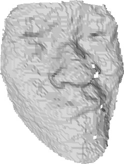
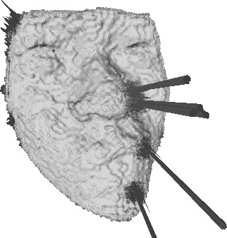
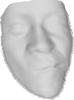
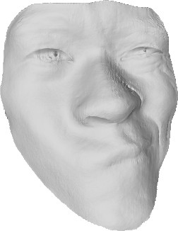
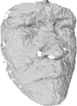
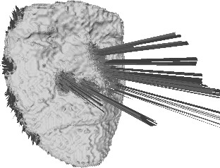
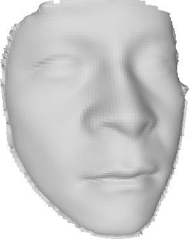
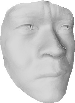
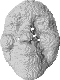
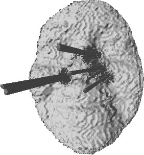
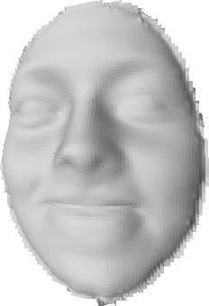
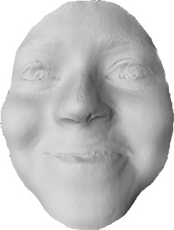
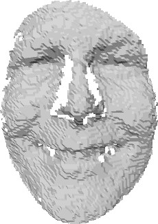
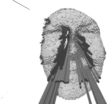
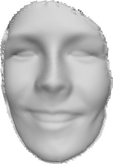
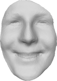
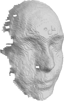
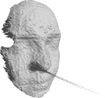
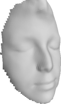
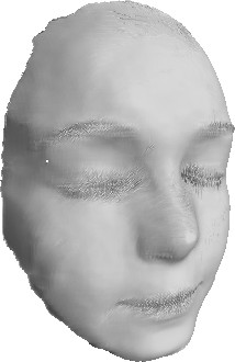
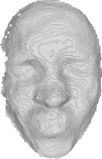
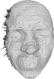
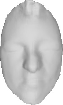
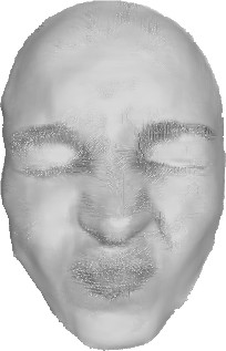
Figure 20: Qualitative comparison of our reflectance learning-based results against state-of-the-art methods, on six RGB-D frames of human faces which we captured using an Intel RealSense D415 camera (scaling factor of $4$). Our method provides the most detailed 3D-reconstructions.

D.4 Comparison against the State-of-the-art on a Public Real-world Dataset

Eventually, we compare qualitatively in Figure 21, and quantitatively in Table IV, the results of the proposed reflectance learning-based approach against those of the state-of-the-art, on data extracted from the DiLiGenT dataset [41]. Note that the datasets are exactly the same as the ones used for the evaluation of the fully variational solution in Figure 15 and Table II, so that the results of the fully variational solution and those of the combined approach can also be compared.

Let us emphasize that the proposed reflectance learning-based solution was trained on a faces dataset, while none of the objects in this experiment resembles a face. Therefore, this test is rather intended as a test of robustness, and we are not expecting to overcome the results of the fully variational solution.

Indeed, the results obtained with the combined approach are both qualitatively and quantitatively less satisfactory on this dataset than those obtained with the fully variational solution. However, they remain surprisingly competitive, in comparison with the state-of-the-art.

Obviously, such a combination of machine learning and variational methods could still be improved by increasing the size of the training database using multiple classes of objects, but the present results already demonstrate its potential.

	$\mathbf{I}$	${z^{0}}$	[62]	[86]	Ours	Ground truth
bear
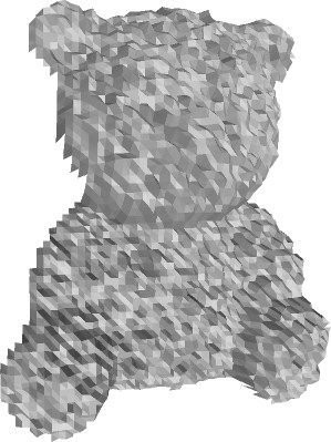
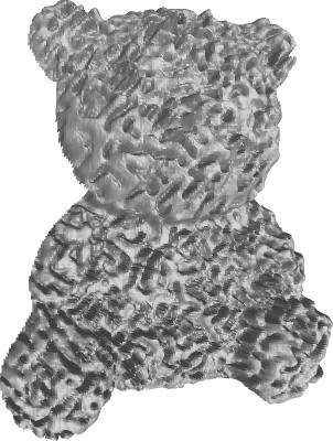
buddha
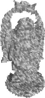
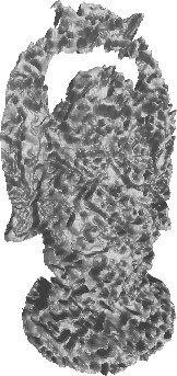
cat
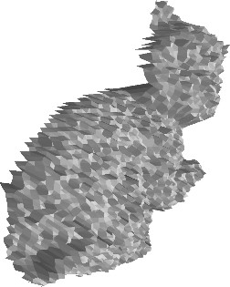
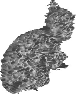
cow
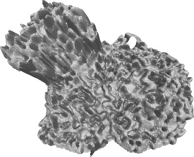
goblet
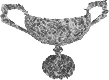
harvest
pot1
pot2
reading

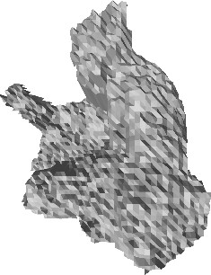
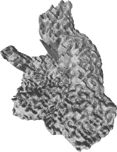
Figure 21: Qualitative comparison between our method combining deep learning and variational methods, and state-of-the-art deep learning-based methods, on the DiLiGenT dataset [41] (the scaling factor is 4). Our approach outperforms the state-of-the-art in all the experiments.

3D-shape	SF	[62]		[86]		Ours
		RMSE	MAE	RMSE	MAE	RMSE	MAE
	2	0.010946	62.708	–	–	0.0046569	22.5961
bear	4	0.010609	49.8753	0.1096	41.9262	0.0086235	23.2417
	8	0.012821	36.8812	–	–	0.018246	30.7021
	2	0.011778	63.0557	–	–	0.0082909	29.6526
buddha	4	0.012539	52.2028	0.0518	40.1120	0.011945	33.5974
	8	0.015423	45.132	–	–	0.019568	41.0636
	2	0.013194	62.903	–	–	0.008389	15.1466
cat	4	0.0137	50.278	0.0647	36.9720	0.013534	19.1494
	8	0.015258	38.3265	–	–	0.023363	26.7149
	2	0.011679	64.5302	–	–	0.0053628	17.6086
cow	4	0.011237	50.6826	0.0562	39.3336	0.0092811	18.8318
	8	0.014157	42.9122	–	–	0.017689	21.1007
	2	0.013153	61.8508	–	–	0.011713	30.1888
goblet	4	0.01379	48.7097	0.1414	36.4712	0.017615	29.6286
	8	0.016659	36.6476	–	–	0.03133	28.7208
	2	0.0167	64.113	–	–	0.016649	39.602
harvest	4	0.019409	53.9958	0.1757	54.1461	0.024208	41.0901
	8	0.028625	44.4953	–	–	0.037441	41.1994
	2	0.011218	61.9779	–	–	0.0070793	18.4819
pot1	4	0.011597	50.0199	0.1051	35.0139	0.010794	18.6248
	8	0.01495	40.4749	–	–	0.019198	20.5408
	2	0.010693	61.9083	–	–	0.0057831	20.0908
pot2	4	0.011123	50.5484	0.0575	32.0884	0.0090011	20.7887
	8	0.014105	40.3902	–	–	0.016243	23.1403
	2	0.012058	61.2583	–	–	0.0098101	20.5263
reading	4	0.012927	49.0756	0.0817	55.4988	0.015531	24.2634
	8	0.017714	41.0243	–	–	0.028793	28.8291
	2	0.011778	62.708	–	–	0.0082909	20.5263
Median	4	0.012539	50.278	0.0732	38.1528	0.011945	23.2417
	8	0.015258	40.4749	–	–	0.019568	28.7208
	2	0.01238	62.7006	–	–	0.0086371	23.766
Mean	4	0.012992	50.5987	0.0918	41.2045	0.013392	25.4684
	8	0.016635	40.6982	–	–	0.023541	29.1124

TABLE IV: Quantitative comparison between other state-of-the-art methods and our method combining machine learning and variational methods. Although the results are not as accurate as the fully variational solution (cf. Table II), since none of the objects here resembles the faces from the training database, they remain superior to the state-of-the-art.

Appendix E Evaluation of the Multi-shot Approach Based on Photometric Stereo

E.1 Creation of the Synthetic Data

In order to quantitatively evaluate the proposed photometric stereo-based solution, we consider the same four 3D-shapes as in the shape-from-shading experiments, i.e. “Lucy”, “Thai Statue”, “Armadillo” and “Joyful Yell”. However, this time we consider much more complex albedo maps since the multi-shot approach is not limited to piecewise-constant albedos. The albedo maps we consider are “ebsd”, “mandala” and “rectcircle”. The rest of the process for creating the dataset (rendering the high-resolution RGB and low-resolution depth images, and adding noise) is exactly the same as for shape-from-shading, except that multiple RGB images are acquired under randomly varying lighting. Three RGB images of each dataset under three different illumination conditions are presented in Figure 22, and the corresponding depth maps are those from Figure 12.

Lucy [100]	Thai Statue [100]	Armadillo [100]	Joyful Yell [101]
“ebsd” albedo	“ebsd” albedo	“mandala” albedo	“rectcircle” albedo

Figure 22: Illustration of the synthetic RGB data used for quantitatively evaluating the multi-shot depth super-resolution approach based on photometric stereo. Each row represents a different illumination condition. Remark that much more complex albedo maps are considered, in comparison with the ones used in the single-shot approach, cf. Figure 12.

E.2 Selecting the Number of Images and Tuning the Hyper-parameters

Figure 23 illustrates the effect of the hyper-parameter $\gamma$ on shape and reflectance estimation. For this purpose, we consider sets of $n=10$ images from the Joyful Yell dataset, and evaluate the RMSE and MAE on depth, as well as the RMSE on albedo, as functions of the number of input images. As can be seen, when $\gamma\to 0$ the estimated depth map sticks to the noisy input, thus results are deceiving. But as soon as $\gamma$ is large enough, photometric stereo drives super-resolution and the accuracy dramatically increases. Interestingly, results remain stable even when $\lambda\to\infty$. This tends to indicate that the ambiguities of uncalibrated photometric stereo vanish as soon as a depth prior is available: it is not necessary to seek a compromise between the depth prior and the photometric 3D-reconstruction, only to plug the information from the former into the latter.

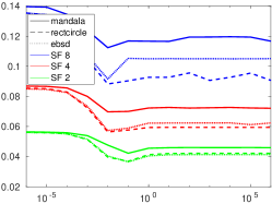
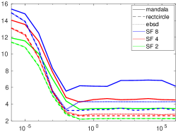
RMSE (depth)		MAE (depth)		RMSE (albedo)
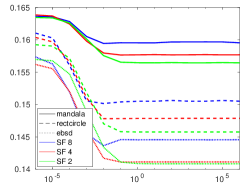
	$\gamma$		$\gamma$		$\gamma$

Figure 23: Impact of the parameter $\gamma$ on the accuracy of the albedo and depth estimates using our multi-shot photometric stereo approach ($n=10$ in this experiment). Based on these results, the value $\gamma=0.01$ was retained.

Next, we evaluate the number $n$ of input RGB images which would result in the best compromise between accuracy of the 3D-reconstruction and runtime. For this purpose, we consider once again the Joyful Yell synthetic dataset, and evaluate the RMSE and MAE on depth, the RMSE on albedo and the total runtime required to attain convergence, as functions of $n$. As can be seen in Figure 24, the accuracy of the estimation very quickly increases with $n$, while the runtime increases linearly with $n$. Overall, the choice $n\in[10,30]$ seems to represent a good compromise.

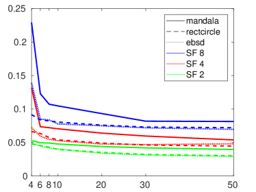
RMSE (depth)		MAE (depth)
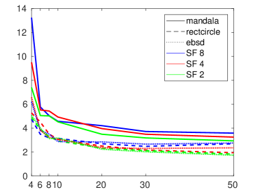
	$n$		$n$
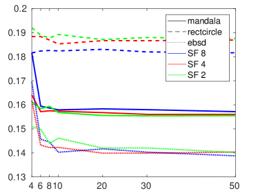
RMSE (albedo)		Runtime ($s$)
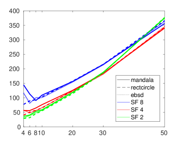
	$n$		$n$

Figure 24: Impact of the number of images $n$ on the accuracy of the albedo and depth estimates using our multi-shot photometric stereo approach ($\gamma=0.01$ in this experiment). The range $n\in[10,30]$ represents a reasonable compromise between accuracy and runtime.

E.3 Comparison against the State-of-the-art on the Synthetic Dataset

Next, we compare our multi-shot approach against the state-of-the-art, on all the synthetic datasets (consistently with the results from the previous subsection, $n=20$ images are considered for each dataset, and $\gamma=0.01$ in all the experiments). Our results are expected to overcome both pure depth super-resolution and pure uncalibrated photometric stereo, as well as single-shot depth refinement methods acting on low-resolution data.

To highlight the interest of an explicit photometric model, we first compare our results against an image-based multi-shot depth super-resolution approach adapted from [91, 1]. It is a personal combination of these papers which achieves variational depth super-resolution by fusing the $n$ low-resolution depth maps, while regularising the gradient of the estimated high-resolution depth map in an anisotropic manner. Here, the anisotropy coefficient is derived from the gradients of the RGB image. This approach is thus a “pure depth super-resolution” one, which uses RGB clues but without any explicit photometric model.

In contrast, we also consider the “pure” uncalibrated photometric stereo method from [37], which estimates lighting, albedo and high-resolution geometry from the $n$ high-resolution RGB images. In this method, an explicit photometric model is used, as in ours, yet no low-resolution depth clue is considered hence the underlying bas-relief ambiguity may affect the quality of the results.

As in the evaluation of the shape-from-shading-based approach from Section C, we also show the results of RGB-D refinement [51] applied to the low-resolution RGB-D frame, selecting one image out of $n$.

The qualitative comparison in Figure 25, and the quantitative ones in Table V, show that our methods result in much more satisfactory high-resolution geometry, in comparison with these methods. This proves that using an explicit model for driving image-based depth super-resolution, and using low-resolution depth clues to disambiguate uncalibrated photometric stereo, both are worthwile.

	Lucy	Thai Statue	Armadillo	Joyful Yell
	“ebsd”	“esbd”	“mandala”	“rectcircle”
[91, 1]
[37]
[51]
Ours

Figure 25: Qualitative comparison of our multi-shot approach against state-of-the-art methods, on four synthetic datasets (scaling factor of 4). Image-based depth super-resolution adapted from [91, 1] results in noisy geometry, uncalibrated photometric stereo results from [37] are slightly flattened due to the underlying bas-relief ambiguity, and RGB-D fusion [51] of the low-resolution data is not really successful here. In comparison, the results of the proposed method are extremely satisfactory.

Albedo	3D-shape	SF	Image Based depth SR		[37]∗		[51]		Ours
			RMSE	MAE	RMSE	MAE	RMSE	MAE	RMSE	MAE
mandala		2	0.031468	46.4149	0.51996	17.4225	0.4320	69.7311	0.023266	2.883
	Armadillo	4	0.042467	43.5403	–	–	0.3948	63.7382	0.037789	2.8391
		8	0.088849	42.6184	–	–	0.5961	83.7853	0.073928	2.9196
		2	0.043889	46.4903	0.37197	15.7192	0.4755	84.6189	0.036334	3.5842
	Lucy	4	0.065857	44.0677	–	–	0.4951	82.0516	0.051316	3.6142
		8	0.12668	42.8905	–	–	0.5231	64.7317	0.084713	4.7864
		2	0.048887	45.0552	1.0735	14.2243	0.3757	70.2724	0.044198	3.3143
	Joyful Yell	4	0.069088	42.644	–	–	0.2985	55.6927	0.063392	3.6407
		8	0.13103	40.0426	–	–	0.4240	44.2549	0.1046	3.753
		2	0.032432	47.8575	0.37738	13.372	0.4615	70.3271	0.022446	3.579
	Thai Statue	4	0.053061	45.5618	–	–	0.4211	90.2134	0.036245	3.6985
		8	0.094911	43.838	–	–	0.3371	53.2791	0.049733	4.1133
rectcircle		2	0.028459	41.506	0.52582	18.0902	0.2844	55.3096	0.020885	2.0047
	Armadillo	4	0.038966	38.7345	–	–	0.3031	48.1000	0.035145	1.9458
		8	0.11182	36.3801	–	–	0.5805	80.4625	0.073139	2.1436
		2	0.040635	42.3051	0.32285	13.6126	0.4868	85.9076	0.026858	1.8617
	Lucy	4	0.062747	39.0783	–	–	0.4685	75.9166	0.041968	2.2851
		8	0.12325	37.956	–	–	0.3767	56.5020	0.075311	3.8793
		2	0.045765	39.9946	0.84162	11.4847	0.2012	41.3053	0.038698	2.7879
	Joyful Yell	4	0.064537	37.1175	–	–	0.3189	37.2107	0.053871	3.1022
		8	0.09492	34.7218	–	–	0.4432	36.3990	0.084381	3.2463
		2	0.030859	44.4276	0.38981	13.3935	0.2625	66.0562	0.018374	2.1086
	Thai Statue	4	0.045516	41.7235	–	–	0.3151	85.4734	0.028457	2.2876
		8	0.10507	39.7697	–	–	0.2389	55.0568	0.041552	3.0519
ebsd		2	0.031939	46.9515	0.49466	16.3427	0.3473	65.4823	0.021037	2.0398
	Armadillo	4	0.04424	44.2571	–	–	0.5933	58.6932	0.036102	2.0035
		8	0.10062	42.2539	–	–	0.6453	81.5187	0.073138	1.8159
		2	0.04299	47.5844	0.32989	13.0463	0.4141	84.9623	0.028555	1.9483
	Lucy	4	0.072388	44.5851	–	–	0.4541	75.3771	0.04325	2.1771
		8	0.16385	42.4252	–	–	0.6460	74.8618	0.079427	3.6839
		2	0.049515	46.0065	1.0052	13.1767	0.2645	55.3462	0.034162	2.1722
	Joyful Yell	4	0.069491	43.4654	–	–	0.2770	42.4242	0.04818	2.3335
		8	0.11255	40.9818	–	–	0.4589	38.8507	0.073515	2.5774
		2	0.03307	48.7666	0.30254	12.0112	0.2371	69.6653	0.019305	2.3639
	Thai Statue	4	0.046843	45.6104	–	–	0.2792	77.7622	0.029185	2.4529
		8	0.089646	43.7591	–	–	0.2847	64.3520	0.041307	2.9642
		2	0.036853	46.2107	0.44223	13.503	0.12186	45.0229	0.025062	2.2681
Median		4	0.057904	43.5029	–	–	0.18929	41.3767	0.039879	2.3932
		8	0.10844	41.6178	–	–	0.31159	41.3102	0.073722	3.1491
		2	0.038326	45.28	0.54626	14.3246	0.11516	42.7392	0.027843	2.554
Mean		4	0.056267	42.5321	–	–	0.18488	40.6331	0.042075	2.6984
		8	0.11193	40.6364	–	–	0.29819	40.1205	0.071228	3.2446

TABLE V: Quantitative comparison of the results attained with the proposed multi-shot approach and the state-of-the-art (^∗: to make the comparison fair, we run the algorithm of [37] on the high resolution RGB images, as it performs uncalibrated photometric stereo on the RGB images without super-resolution – the scaling factor is thus actually 1 in this case). Our approach overcomes the state-of-the-art in all the experiments.

E.4 Qualitative Comparison against the State-of-the-art on Real-world Datasets we Captured Ourselves

Figure 26 shows four qualitative comparisons against the state-of-the-art, on real-world data from Figures 1 and 6 in the main paper, which was captured with an Asus Xtion Pro Live camera (scaling factor of 4).

It can be seen that image-based depth super-resolution approach hallucinates reflectance information as geometric information, since the underlying concept allows larger depth variations where strong image gradients are present. The uncalibrated photometric stereo results from [37] contain much more relevant details, but the approach clearly suffers from a low-frequency bias due to the underlying bas-relief ambiguity, cf. “Tablet Case” and “Vase”. In these experiments the RGB-D fusion results from [51] are reasonable, but not as accurate as the ones obtained with the proposed multi-shot approach.

	One of $\mathbf{I}_{i}$	${z^{0}}$	[91, 1]	[37]	[51]	Ours
Tablet Case
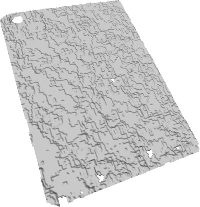
Vase
Shirt
Backpack

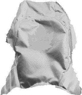
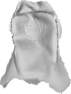
Figure 26: Comparison between the proposed multi-shot method and the state-of-the-art, on real-world datasets captured using an Asus Xtion Pro Live camera. These results confirm the conclusion of the synthetic experiments in Figure 25. 
 

E.5 Comparison against the State-of-the-art on a Public Real-world Dataset

Eventually, we compare our results against the state-of-the-art on the DiLiGenT dataset [41]. Qualitative results are presented in Figure 27, and quantitative ones in Table VI. Once again, our method most of the times overcomes the state-of-the art in terms of surface details recovery. It is also interesting to compare these results with the corresponding ones in the previous sections: this comparison clearly shows that resorting to a multi-shot strategy based on photometric stereo is the only way to cope with general reflectance.

Still, it can be observed that even with redundant data, some results such as the “harvest” one remain somewhat disappointing: this is because the proposed method explicitly builds upon the Lambertian assumption, which is not met in this example. Future extensions could thus include coping with non-Lambertian phenomena.

	One of $\mathbf{I}_{i}$	${z^{0}}$	[91, 1]	[37]	Ours	GT
bear
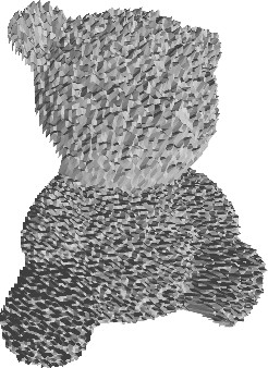
buddha
cat
cow
goblet
harvest
pot1
pot2
reading

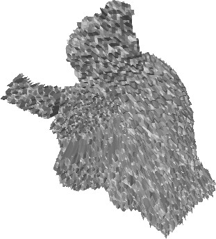
Figure 27: Qualitative comparison of our uncalibrated photometric stereo-based approach against state-of-the-art methods, on the DiLiGenT dataset [41] (the scaling factor is $2$). Our method overcomes the state-of-the-art in all the experiments.

3D-shape	SF	[91, 1]		[37]∗		Ours
		RMSE	MAE	RMSE	MAE	RMSE	MAE
	2	0.0077882	23.2799	0.029124	8.65	0.0064907	7.056
bear	4	0.0077919	19.6628	–	–	0.0083983	7.2645
	8	0.0079796	23.8495	–	–	0.013453	7.0708
	2	0.0077863	31.0075	0.041827	18.0718	0.0066078	12.7816
buddha	4	0.0078303	28.5663	–	–	0.0077671	13.0276
	8	0.0076309	20.1206	–	–	0.012959	13.6987
	2	0.0078205	24.5162	0.039112	11.0118	0.008108	6.1952
cat	4	0.0076492	20.6365	–	–	0.010542	6.5739
	8	0.0078364	21.2045	–	–	0.015403	7.3812
	2	0.0078497	31.5175	0.030244	18.1343	0.0055052	10.4445
cow	4	0.007844	26.7532	–	–	0.0083455	11.3151
	8	0.0085472	17.225	–	–	0.015231	12.7818
	2	0.0078938	32.2235	0.13005	71.5669	0.010771	11.16
goblet	4	0.0078725	29.261	–	–	0.015434	11.6484
	8	0.008322	24.9651	–	–	0.030694	13.9542
	2	0.0078757	32.6288	0.06847	29.3081	0.024211	30.4736
harvest	4	0.0078363	30.6866	–	–	0.029344	31.9109
	8	0.0077605	33.427	–	–	0.040837	33.5636
	2	0.0078648	25.4586	0.01869	10.3055	0.0063032	7.3048
pot1	4	0.0078397	22.6612	–	–	0.0080599	7.514
	8	0.0079306	30.9277	–	–	0.014455	7.9022
	2	0.0077881	29.7433	0.022896	14.5031	0.0048177	9.4492
pot2	4	0.0080123	26.261	–	–	0.0066391	9.5829
	8	0.0076366	21.8009	–	–	0.012587	10.0768
	2	0.0077277	29.1401	0.069057	25.0014	0.0098433	16.7382
reading	4	0.0076277	26.4486	–	–	0.014885	19.6366
	8	0.0078612	18.6829	–	–	0.027963	23.2138
	2	0.0078205	29.7433	0.039112	18.0718	0.0066078	10.4445
Median	4	0.0078363	26.4486	–	–	0.0083983	11.3151
	8	0.0078612	21.8009	–	–	0.015231	12.7818
	2	0.0078216	28.835	0.049941	22.9503	0.0091842	12.4004
Mean	4	0.0078115	25.6597	–	–	0.012157	13.1638
	8	0.007945	23.5781	–	–	0.020398	14.4048

TABLE VI: Quantitative Comparison between other state-of-the-art methods and our multi-shot approach based on photometric stereo (^∗: to make the comparison fair, we run the algorithm of [37] on the high resolution RGB images, as it performs uncalibrated photometric stereo on the RGB images without super-resolution – the scaling factor is thus actually equal to 1 in this case). Our approach overcomes the state-of-the-art in terms of the level of geometric details which can be recovered, while being only slightly less accurate in terms of overall RMSE fit.

Appendix F Unified Comparison of our Results on a Public Real-world Dataset

Eventually, we present in Figure 28 a unified qualitative comparison of the results obtained with the three proposed methods, on the $9$ objects of the DiLiGenT dataset [41]. This dataset illustrates well the cases where the single-shot approach can be used (when reflectance is uniform, as for instance in the “bear” example) and when it completely fails because the piecewise-constant albedo assumption is not satisfied (e.g., “Cat”). This method could thus still be improved by designing a more general reflectance prior. The multi-shot approach based on uncalibrated photometric stereo estimates a much more reasonable albedo map, and thus a much more satisfactory depth map, because it does not rely on any assumption regarding piecewise-constantness. Yet, it could still be improved in order to reduce artifacts due to specularirites (e.g., “reading”). Eventually, the albedo estimated by deep learning is sometimes reasonable (e.g., “buddha”), but most of the times it is not really satisfactory. This is because the objects do not resemble the training set, which consists only of faces: to cope with a wider variety of objects, the training dataset should contain a broader range of object classes.

	Input $\{\mathbf{I},{z^{0}}\}$	SfS	SfS + reflectance learning	UPS
bear
buddha
cat
cow

	Input $\{\mathbf{I},{z^{0}}\}$	SfS	SfS + reflectance learning	UPS
goblet
harvest
pot1
pot2
reading

Figure 28: Comparison of the albedo and high-resolution depth maps estimated by the proposed variational approach to shape-from-shading (SfS), the combination of SfS and deep reflectance learning, and the uncalibrated photometric stereo (UPS)-based approach, on the DiLiGenT dataset [41]. For quantitative evaluation, we refer the reader to Tables II, IV and VI.  
 

Appendix G Conclusion

We evaluated in depth the applicability of photometric techniques to resolve depth super-resolution in the context of RGB-D sensing. Multiple self-captured real-world, publicly available real-world and self-generated synthetic datasets were used in order to qualitatively and quantitatively compare the three proposed strageties against state-of-the-art variational, optimization-based and deep learning methods. It appeared that each of the three proposed methods beats the corresponding state-of-the-art ones, which provides an empirical evidence for the soundness of considering photometry as a valuable clue for depth super-resolution in RGB-D sensing.

In order to have at hand a unified comparison of the three methods presented in this work, we also considered a publicly available real-world photometric stereo benchmark across all experimental sections. This permitted us to clearly highlight the respective strengths and weaknesses of each method. They could still be improved towards, respectively, a more general reflectance prior (single-shot strategy), a broader training dataset (reflectance learning), and the handling of specularities (uncalibrated photometric stereo).

References

- [1] M. Unger, T. Pock, M. Werlberger, and H. Bischof, “A convex approach for variational super-resolution,” in Joint Pattern Recognition Symposium, 2010, pp. 313–322.
- [2] J. Park, H. Kim, Y.-W. Tai, M. S. Brown, and I. S. Kweon, “High quality depth map upsampling for 3F-TOF cameras,” in Proceedings of the IEEE International Conference on Computer Vision (ICCV), 2011, pp. 1623–1630.
- [3] Y. Quéau, J.-D. Durou, and J.-F. Aujol, “Normal Integration: A Survey,” Journal of Mathematical Imaging and Vision, vol. 60, no. 4, pp. 576–593, 2018.
- [4] R. Basri and D. P. Jacobs, “Lambertian reflectances and linear subspaces,” IEEE Transactions on Pattern Analysis and Machine Intelligence, vol. 25, no. 2, pp. 218–233, 2003.
- [5] R. Ramamoorthi and P. Hanrahan, “An Efficient Representation for Irradiance Environment Maps,” in Proceedings of the Annual Conference on Computer Graphics and Interactive Techniques, 2001, pp. 497–500.
- [6] B. Goldlücke, M. Aubry, K. Kolev, and D. Cremers, “A super-resolution framework for high-accuracy multiview reconstruction,” International Journal of Computer Vision, vol. 106, no. 2, pp. 172–191, 2014.
- [7] R. Maier, J. Stückler, and D. Cremers, “Super-resolution keyframe fusion for 3D modeling with high-quality textures,” in Proceedings of the International Conference on 3D Vision (3DV), 2015, pp. 536–544.
- [8] S. Schuon, C. Theobalt, J. Davis, and S. Thrun, “Lidarboost: Depth superresolution for TOF 3D shape scanning,” in Proceedings of the IEEE Conference on Computer Vision and Pattern Recognition (CVPR), 2009, pp. 343–350.
- [9] O. Mac Aodha, N. D. F. Campbell, A. Nair, and G. J. Brostow, “Patch based synthesis for single depth image super-resolution,” in Proceedings of the European Conference on Computer Vision (ECCV), 2012, pp. 71–84.
- [10] J. Xie, R. S. Feris, and M.-T. Sun, “Edge-guided single depth image super resolution,” IEEE Transactions on Image Processing, vol. 25, no. 1, pp. 428–438, 2016.
- [11] M. Hornácek, C. Rhemann, M. Gelautz, and C. Rother, “Depth super resolution by rigid body self-similarity in 3D,” in Proceedings of the IEEE Conference on Computer Vision and Pattern Recognition (CVPR), 2013, pp. 1123–1130.
- [12] J. Li, Z. Lu, G. Zeng, R. Gan, and H. Zha, “Similarity-aware patchwork assembly for depth image super-resolution,” in Proceedings of the IEEE Conference on Computer Vision and Pattern Recognition (CVPR), 2014, pp. 3374–3381.
- [13] J. Xie, R. S. Feris, S.-S. Yu, and M.-T. Sun, “Joint super resolution and denoising from a single depth image,” IEEE Transactions on Multimedia, vol. 17, no. 9, pp. 1525–1537, 2015.
- [14] D. Ferstl, M. Rüther, and H. Bischof, “Variational depth superresolution using example-based edge representations,” in Proceedings of the IEEE International Conference on Computer Vision (ICCV), 2015, pp. 513–521.
- [15] G. Riegler, M. Rüther, and H. Bischof, “ATGV-net: accurate depth super-resolution,” in Proceedings of the European Conference on Computer Vision (ECCV), 2016, pp. 268–284.
- [16] B. K. P. Horn, “Shape From Shading: A Method for Obtaining the Shape of a Smooth Opaque Object From One View,” Ph.D. dissertation, Department of Electrical Engineering and Computer Science, Massachusetts Institute of Technology, 1970.
- [17] M. Breuß, E. Cristiani, J.-D. Durou, M. Falcone, and O. Vogel, “Perspective shape from shading: Ambiguity analysis and numerical approximations,” SIAM Journal on Imaging Sciences, vol. 5, no. 1, pp. 311–342, 2012.
- [18] J.-D. Durou, M. Falcone, and M. Sagona, “Numerical Methods for Shape-from-shading: A New Survey with Benchmarks,” Computer Vision and Image Understanding, vol. 109, no. 1, pp. 22–43, 2008.
- [19] R. Zhang, P.-S. Tsai, J. E. Cryer, and M. Shah, “Shape-from-shading: a survey,” IEEE Transactions on Pattern Analysis and Machine Intelligence, vol. 21, no. 8, pp. 690–706, 1999.
- [20] B. K. P. Horn and M. J. Brooks, “The variational approach to shape from shading,” Computer Vision, Graphics, and Image Processing, vol. 33, no. 2, pp. 174–208, 1986.
- [21] K. Ikeuchi and B. K. Horn, “Numerical shape from shading and occluding boundaries,” Artificial intelligence, vol. 17, no. 1-3, pp. 141–184, 1981.
- [22] E. Cristiani and M. Falcone, “Fast semi-lagrangian schemes for the eikonal equation and applications,” SIAM Journal on Numerical Analysis, vol. 45, no. 5, pp. 1979–2011, 2007.
- [23] M. Falcone and M. Sagona, “An algorithm for the global solution of the shape-from-shading model,” in Proceedings of the International Conference on Image Analysis and Processing (ICIAP), 1997, pp. 596–603.
- [24] P.-L. Lions, E. Rouy, and A. Tourin, “Shape-from-shading, viscosity solutions and edges,” Numerische Mathematik, vol. 64, no. 1, pp. 323–353, 1993.
- [25] E. Rouy and A. Tourin, “A viscosity solutions approach to shape-from-shading,” SIAM Journal on Numerical Analysis, vol. 29, no. 3, pp. 867–884, 1992.
- [26] E. H. Adelson and A. P. Pentland, Perception as Bayesian inference. Cambridge University Press, 1996, ch. The perception of shading and reflectance, pp. 409–423.
- [27] R. Huang and W. A. P. Smith, “Shape-from-shading under complex natural illumination,” in Proceedings of the IEEE International Conference on Image Processing (ICIP), 2011, pp. 13–16.
- [28] M. K. Johnson and E. H. Adelson, “Shape estimation in natural illumination,” in Proceedings of the IEEE Conference on Computer Vision and Pattern Recognition (CVPR), 2011, pp. 2553–2560.
- [29] S. R. Richter and S. Roth, “Discriminative shape from shading in uncalibrated illumination,” in Proceedings of the IEEE Conference on Computer Vision and Pattern Recognition (CVPR), 2015, pp. 1128–1136.
- [30] Y. Quéau, J. Mélou, F. Castan, D. Cremers, and J.-D. Durou, “A Variational Approach to Shape-from-shading Under Natural Illumination,” in Energy Minimization Methods for Computer Vision and Pattern Recognition (EMMCVPR), 2017, pp. 342–357.
- [31] J. Barron and J. Malik, “Shape, illumination, and reflectance from shading,” IEEE Transactions on Pattern Analysis and Machine Intelligence, vol. 37, no. 8, pp. 1670–1687, 2015.
- [32] R. J. Woodham, “Photometric Method for Determining Surface Orientation from Multiple Images,” Optical Engineering, vol. 19, no. 1, pp. 139–144, 1980.
- [33] H. Hayakawa, “Photometric stereo under a light source with arbitrary motion,” Journal of the Optical Society of America A, vol. 11, no. 11, pp. 3079–3089, 1994.
- [34] P. N. Belhumeur, D. J. Kriegman, and A. L. Yuille, “The bas-relief ambiguity,” International Journal of Computer Vision, vol. 35, no. 1, pp. 33–44, 1999.
- [35] R. Basri, D. W. Jacobs, and I. Kemelmacher, “Photometric stereo with general, unknown lighting,” International Journal of Computer Vision, vol. 72, no. 3, pp. 239–257, 2007.
- [36] N. G. Alldrin, S. P. Mallick, and D. J. Kriegman, “Resolving the generalized bas-relief ambiguity by entropy minimization,” in Proceedings of the IEEE Conference on Computer Vision and Pattern Recognition (CVPR), 2007.
- [37] T. Papadhimitri and P. Favaro, “A closed-form, consistent and robust solution to uncalibrated photometric stereo via local diffuse reflectance maxima,” International Journal of Computer Vision, vol. 107, no. 2, pp. 139–154, 2014.
- [38] Y. Quéau, F. Lauze, and J.-D. Durou, “Solving Uncalibrated Photometric Stereo using Total Variation,” Journal of Mathematical Imaging and Vision, vol. 52, no. 1, pp. 87–107, 2015.
- [39] F. Lu, X. Chen, I. Sato, and Y. Sato, “Symps: Brdf symmetry guided photometric stereo for shape and light source estimation,” IEEE Transactions on Pattern Analysis and Machine Intelligence, vol. 40, no. 1, pp. 221–234, 2018.
- [40] Z. Mo, B. Shi, F. Lu, S.-K. Yeung, and Y. Matsushita, “Uncalibrated photometric stereo under natural illumination,” in Proceedings of the IEEE Conference on Computer Vision and Pattern Recognition (CVPR), 2018, pp. 2936–2945.
- [41] B. Shi, Z. Mo, Z. Wu, D. Duan, S. K. Yeung, and P. Tan, “A benchmark dataset and evaluation for non-lambertian and uncalibrated photometric stereo,” IEEE Transactions on Pattern Analysis and Machine Intelligence, vol. 41, no. 2, pp. 271–284, 2019.
- [42] Y. Quéau, T. Wu, F. Lauze, J.-D. Durou, and D. Cremers, “A Non-Convex Variational Approach to Photometric Stereo under Inaccurate Lighting,” in Proceedings of the IEEE Conference on Computer Vision and Pattern Recognition (CVPR), 2017, pp. 350–359.
- [43] S. Ikehata, “CNN-PS: CNN-based photometric stereo for general non-convex surfaces,” in Proceedings of the European Conference on Computer Vision (ECCV), 2018, pp. 3–18.
- [44] G. Chen, K. Han, B. Shi, Y. Matsushita, and K.-Y. K. Wong, “Self-calibrating deep photometric stereo networks,” in Proceedings of the IEEE Conference on Computer Vision and Pattern Recognition (CVPR), 2019.
- [45] G. Choe, J. Park, Y.-W. Tai, and I. S. Kweon, “Refining geometry from depth sensors using IR shading images,” International Journal of Computer Vision, vol. 122, no. 1, pp. 1–16, 2017.
- [46] R. Maier, K. Kim, D. Cremers, J. Kautz, and M. Nießner, “Intrinsic3d: High-quality 3D reconstruction by joint appearance and geometry optimization with spatially-varying lighting,” in Proceedings of the IEEE International Conference on Computer Vision (ICCV), 2017, pp. 3114–3122.
- [47] M. Zollhöfer, A. Dai, M. Innman, C. Wu, M. Stamminger, C. Theobalt, and M. Nießner, “Shading-based refinement on volumetric signed distance functions,” ACM Transactions on Graphics, vol. 34, no. 4, pp. 96:1–96:14, 2015.
- [48] Y. Han, J.-Y. Lee, and I. S. Kweon, “High Quality Shape from a Single RGB-D Image under Uncalibrated Natural Illumination,” in Proceedings of the IEEE International Conference on Computer Vision (ICCV), 2013, pp. 1617–1624.
- [49] K. Kim, A. Torii, and M. Okutomi, “Joint estimation of depth, reflectance and illumination for depth refinement,” in Proceedings of the IEEE International Conference on Computer Vision (ICCV), 2015, pp. 199–207.
- [50] R. Or-El, R. Hershkovitz, A. Wetzler, G. Rosman, A. M. Bruckstein, and R. Kimmel, “Real-time depth refinement for specular objects,” in Proceedings of the IEEE Conference on Computer Vision and Pattern Recognition (CVPR), 2016, pp. 4378–4386.
- [51] R. Or-El, G. Rosman, A. Wetzler, R. Kimmel, and A. Bruckstein, “RGBD-Fusion: Real-Time High Precision Depth Recovery,” in Proceedings of the IEEE Conference on Computer Vision and Pattern Recognition (CVPR), 2015, pp. 5407–5416.
- [52] C. Wu, M. Zollhöfer, M. Nießner, M. Stamminger, S. Izadi, and C. Theobalt, “Real-time shading-based refinement for consumer depth cameras,” ACM Transactions on Graphics, vol. 33, no. 6, pp. 200:1–200:10, 2014.
- [53] L.-F. Yu, S.-K. Yeung, Y.-W. Tai, and S. Lin, “Shading-based shape refinement of RGB-D images,” in Proceedings of the IEEE Conference on Computer Vision and Pattern Recognition (CVPR), 2013, pp. 1415–1422.
- [54] R. Anderson, B. Stenger, and R. Cipolla, “Augmenting depth camera output using photometric stereo,” in Proceedings of the IAPR Conference on Machine Vision Applications (MVA), 2011, pp. 369–372.
- [55] A. Chatterjee and V. Madhav Govindu, “Photometric refinement of depth maps for multi-albedo objects,” in Proceedings of the IEEE Conference on Computer Vision and Pattern Recognition (CVPR), 2015, pp. 933–941.
- [56] L. Xie, Y. Xu, X. Zhang, W. Bao, C. Tong, and B. Shi, “A self-calibrated photo-geometric depth camera,” The Visual Computer, 2018.
- [57] Y. Zhang, Q. Zhang, and W. Feng, “High-Resolution Depth Refinement by Photometric and Multi-shading Constraints,” in PRICAI 2018: Trends in Artificial Intelligence, 2018, pp. 201–209.
- [58] J. Diebel and S. Thrun, “An application of Markov random fields to range sensing,” in Advances in Neural Information Processing Systems, 2006, pp. 291–298.
- [59] D. Ferstl, C. Reinbacher, R. Ranftl, M. Rüther, and H. Bischof, “Image guided depth upsampling using anisotropic total generalized variation,” in Proceedings of the IEEE International Conference on Computer Vision (ICCV), 2013, pp. 993–1000.
- [60] Q. Yang, R. Yang, J. Davis, and D. Nistér, “Spatial-depth super resolution for range images,” in Proceedings of the IEEE Conference on Computer Vision and Pattern Recognition (CVPR), 2007.
- [61] B. Li, Y. Zhou, Y. Zhang, and A. Wang, “Depth image super-resolution based on joint sparse coding,” Pattern Recognition Letters, 2019, (in press).
- [62] T.-W. Hui, C. C. Loy, and X. Tang, “Depth map super-resolution by deep multi-scale guidance,” in Proceedings of European Conference on Computer Vision (ECCV), 2016, pp. 353–369.
- [63] P. Tan, S. Lin, and L. Quan, “Subpixel photometric stereo,” IEEE Transactions on Pattern Analysis and Machine Intelligence, vol. 30, no. 8, pp. 1460–1471, 2008.
- [64] S. Chaudhuri and M. V. Joshi, Motion-free super-resolution. Springer Verlag, 2005.
- [65] Z. Lu, Y.-W. Tai, F. Deng, M. Ben-Ezra, and M. S. Brown, “A 3D imaging framework based on high-resolution photometric-stereo and low-resolution depth,” International Journal of Computer Vision, vol. 102, no. 1-3, pp. 18–32, 2013.
- [66] B. Haefner, Y. Quéau, T. Möllenhoff, and D. Cremers, “Fight ill-posedness with ill-posedness: Single-shot variational depth super-resolution from shading,” in Proceedings of the IEEE Conference on Computer Vision and Pattern Recognition (CVPR), 2018, pp. 164–174.
- [67] S. Peng, B. Haefner, Y. Quéau, and D. Cremers, “Depth super-resolution meets uncalibrated photometric stereo,” in Proceedings of the IEEE International Conference on Computer Vision (ICCV) Workshops, 2017, pp. 2961–2968.
- [68] D. Mumford, “Bayesian rationale for the variational formulation,” in Geometry-driven diffusion in computer vision, 1994, pp. 135–146.
- [69] G. Graber, J. Balzer, S. Soatto, and T. Pock, “Efficient minimal-surface regularization of perspective depth maps in variational stereo,” in Proceedings of the IEEE Conference on Computer Vision and Pattern Recognition (CVPR), 2015, pp. 511–520.
- [70] E. H. Land, “The retinex theory of color vision,” Scientific American, vol. 237, no. 6, pp. 108–120, 1977.
- [71] S. Boyd, N. Parikh, E. Chu, B. Peleato, and J. Eckstein, “Distributed Optimization and Statistical Learning via the Alternating Direction Method of Multipliers,” Foundations and Trends in Machine Learning, vol. 3, no. 1, pp. 1–122, 2011.
- [72] J. Eckstein and D. P. Bertsekas, “On the Douglas–Rachford splitting method and the proximal point algorithm for maximal monotone operators,” Mathematical Programming, vol. 55, no. 1, pp. 293–318, 1992.
- [73] R. Glowinski and A. Marroco, “Sur l’approximation, par éléments finis d’ordre un, et la résolution, par pénalisation-dualité d’une classe de problèmes de Dirichlet non linéaires,” Revue française d’automatique, informatique, recherche opérationnelle. Analyse numérique, vol. 9, no. R2, pp. 41–76, 1975.
- [74] E. Strekalovskiy and D. Cremers, “Real-time minimization of the piecewise smooth Mumford-Shah functional,” in Proceedings of the European Conference on Computer Vision (ECCV), 2014, pp. 127–141.
- [75] M. Schmidt, “minFunc: unconstrained differentiable multivariate optimization in Matlab,” 2005, http://www.cs.ubc.ca/~schmidtm/Software/minFunc.html.
- [76] D. C. Liu and J. Nocedal, “On the limited memory BFGS method for large scale optimization,” Mathematical programming, vol. 45, no. 1, pp. 503–528, 1989.
- [77] “inpaint_nans,” 2012, https://fr.mathworks.com/matlabcentral/fileexchange/4551-inpaint_nans.
- [78] K. He, J. Sun, and X. Tang, “Guided image filtering,” IEEE Transactions on Pattern Analysis and Machine Intelligence, no. 6, pp. 1397–1409, 2013.
- [79] J. Shen, X. Yang, Y. Jia, and X. Li, “Intrinsic images using optimization,” in Proceedings of the IEEE Conference on Computer Vision and Pattern Recognition (CVPR), 2011, pp. 3481–3487.
- [80] Q. Fan, J. Yang, G. Hua, B. Chen, and D. Wipf, “Revisiting deep intrinsic image decompositions,” in Proceedings of The IEEE Conference on Computer Vision and Pattern Recognition (CVPR), 2018, pp. 8944–8952.
- [81] C. Li, K. Zhou, and S. Lin, “Intrinsic face image decomposition with human face priors,” in Proceedings of the European Conference on Computer Vision (ECCV), 2014, pp. 218–233.
- [82] D. Eigen, C. Puhrsch, and R. Fergus, “Depth map prediction from a single image using a multi-scale deep network,” in Advances in Neural Information Processing Systems, 2014, pp. 2366–2374.
- [83] G. Trigeorgis, P. Snape, I. Kokkinos, and S. Zafeiriou, “Face normals ”in-the-wild” using fully convolutional networks,” in Proceedings of the IEEE Conference on Computer Vision and Pattern Recognition (CVPR), 2017, pp. 38–47.
- [84] Z. Shu, E. Yumer, S. Hadap, K. Sunkavalli, E. Shechtman, and D. Samaras, “Neural face editing with intrinsic image disentangling,” in Proceedings of the IEEE Conference on Computer Vision and Pattern Recognition (CVPR), 2017, pp. 5444–5453.
- [85] N. Wang, Y. Zhang, Z. Li, Y. Fu, W. Liu, and Y.-G. Jiang, “Pixel2mesh: Generating 3d mesh models from single rgb images,” in Proceedings of the European Conference on Computer Vision (ECCV), 2018.
- [86] S. Sengupta, A. Kanazawa, C. D. Castillo, and D. W. Jacobs, “SfSNet: Learning Shape, Refectance and Illuminance of Faces in the Wild,” in Proceedings of the IEEE Conference on Computer Vision and Pattern Recognition (CVPR), 2018, pp. 6296–6305.
- [87] J. Shi, Y. Dong, H. Su, and S. X. Yu, “Learning non-lambertian object intrinsics across shapenet categories,” in Proceedings of the IEEE Conference on Computer Vision and Pattern Recognition (CVPR), 2017, pp. 5844–5853.
- [88] W.-C. Ma, T. Hawkins, P. Peers, C.-F. Chabert, M. Weiss, and P. Debevec, “Rapid acquisition of specular and diffuse normal maps from polarized spherical gradient illumination,” in Proceedings of the 18th Eurographics Conference on Rendering Techniques, 2007, pp. 183–194.
- [89] G. Stratou, A. Ghosh, P. Debevec, and L. Morency, “Effect of illumination on automatic expression recognition: A novel 3d relightable facial database,” in Face and Gesture, 2011, pp. 611–618.
- [90] O. Ronneberger, P. Fischer, and T. Brox, “U-net: Convolutional networks for biomedical image segmentation,” in Medical Image Computing and Computer-Assisted Intervention (MICCAI), 2015, pp. 234–241.
- [91] M. Werlberger, W. Trobin, T. Pock, A. Wedel, D. Cremers, and H. Bischof, “Anisotropic Huber-L1 Optical Flow,” in Proceedings of the British Machine Vision Conference, 2009, pp. 108.1–108.11.
- [92] L. Chen, Y. Zheng, B. Shi, A. Subpa-Asa, and I. Sato, “A microfacet-based reflectance model for photometric stereo with highly specular surfaces,” in Proceedings of the IEEE International Conference on Computer Vision (ICCV), 2017, pp. 3162–3170.
- [93] M.-A. Gardner, K. Sunkavalli, E. Yumer, X. Shen, E. Gambaretto, C. Gagné, and J.-F. Lalonde, “Learning to predict indoor illumination from a single image,” ACM Transactions on Graphics, vol. 36, no. 6, pp. 176:1–176:14, 2017.
- [94] Y. Quéau, B. Durix, T. Wu, D. Cremers, F. Lauze, and J.-D. Durou, “LED-based Photometric Stereo: Modeling, Calibration and Numerical Solution,” Journal of Mathematical Imaging and Vision, vol. 60, no. 3, pp. 313–340, 2018.
- [95] D. Frolova, D. Simakov, and R. Basri, “Accuracy of spherical harmonic approximations for images of Lambertian objects under far and near lighting,” in Proceedings of the European Conference on Computer Vision (ECCV), 2004, pp. 574–587.
- [96] M. M. Takuya Narihira and S. X. Yu, “Direct intrinsics: Learning albedo-shading decomposition by convolutional regression,” in Proceedings of the IEEE International Conference on Computer Vision (ICCV), 2015.
- [97] D. J. Butler, J. Wulff, G. B. Stanley, and M. J. Black, “A naturalistic open source movie for optical flow evaluation,” in Proceedings of the European Conference on Computer Vision (ECCV), 2012, pp. 611–625.
- [98] R. Grosse, M. K. Johnson, E. H. Adelson, and W. T. Freeman, “Ground truth dataset and baseline evaluations for intrinsic image algorithms,” in Proceedings of the IEEE International Conference on Computer Vision (ICCV), 2009, pp. 2335–2342.
- [99] A. X. Chang, T. Funkhouser, L. Guibas, P. Hanrahan, Q. Huang, Z. Li, S. Savarese, M. Savva, S. Song, H. Su, J. Xiao, L. Yi, and F. Yu, “ShapeNet: An Information-Rich 3D Model Repository,” Stanford University — Princeton University — Toyota Technological Institute at Chicago, Tech. Rep. arXiv:1512.03012 [cs.GR], 2015.
- [100] M. Levoy, J. Gerth, B. Curless, and K. Pull, “The stanford 3d scanning repository,” 2005, http://www-graphics.stanford.edu/data/3dscanrep.
- [101] “The joyful yell,” 2015, https://www.thingiverse.com/thing:897412.
- [102] K. Khoshelham and S. O. Elberink, “Accuracy and resolution of Kinect depth data for indoor mapping applications,” Sensors, vol. 12, no. 2, pp. 1437–1454, 2012.
- [103] Z. Wang and A. C. Bovik, “Mean squared error: Love it or leave it? a new look at signal fidelity measures,” IEEE signal processing magazine, vol. 26, no. 1, pp. 98–117, 2009.
- [104] R. Maier, K. Kim, D. Cremers, J. Kautz, and M. Nießner, “Intrinsic3D Dataset,” 2017, http://vision.in.tum.de/data/datasets/intrinsic3d.
- [105] Y. Quéau, J.-D. Durou, and J.-F. Aujol, “Variational methods for normal integration,” Journal of Mathematical Imaging and Vision, vol. 60, no. 4, pp. 609–632, 2018.