First–order mean motion resonances in two–planet systems: general analysis and observed systems

Abstract

This paper focuses on two–planet systems in a first–order $(q+1):q$ mean motion resonance and undergoing type–I migration in a disc. We present a detailed analysis of the resonance valid for any value of $q$. Expressions for the equilibrium eccentricities, mean motions and departure from exact resonance are derived in the case of smooth convergent migration. We show that this departure, not assumed to be small, is such that period ratio normally exceeds, but can also be less than, $(q+1)/q.$ Departure from exact resonance as a function of time for systems starting in resonance and undergoing divergent migration is also calculated. We discuss observed systems in which two low mass planets are close to a first–order resonance. We argue that the data are consistent with only a small fraction of the systems having been captured in resonance. Furthermore, when capture does happen, it is not in general during smooth convergent migration through the disc but after the planets reach the disc inner parts. We show that although resonances may be disrupted when the inner planet enters a central cavity, this alone cannot explain the spread of observed separations. Disruption is found to result in either the system moving interior to the resonance by a few percent, or attaining another resonance. We postulate two populations of low mass planets: a small one for which extensive smooth migration has occurred, and a larger one that formed approximately in–situ with very limited migration.

1 Introduction

The orbital architecture of extrasolar planetary systems has been the focus of many studies since Lissauer et al. (2011) published the first statistical analysis of Kepler multiplanet systems based on the first four months of mission data. They reported that most of the systems were not in or close to mean motion resonances (MMRs), but that at the same time there was a significant excess of planet pairs near MMRs. These results were later confirmed by Fabrycky et al. (2014) using the first six quarters of Kepler data, who in addition pointed out that planet pairs near MMRs tend to be preferentially wide of exact resonance.

Because of observational bias, the planets detected by Kepler are on short period orbits. They have either formed further away and migrated over a large distance down to the disc inner parts, or undergone only modest convergent migration, possibly forming in–situ. If the outer planet is the more massive migration usually leads to resonant capture, either while the planets migrate through the disc, or after they reach a cavity interior to the disc. In the former case the commensurability is expected to be maintained while the planets continue to migrate.

Such a scenario leads to a probability of capture which is much higher than indicated by the data (Izidoro et al. 2017), although resonances may be overstable and therefore not permanent when the forced eccentricities are large enough (Goldreich & Schlichting 2014, Hands & Alexander 2018). In–situ formation leads to systems which are not preferentially in resonances (Hansen & Murray 2013). Petrovich et al. (2013) note that two planet systems that appear for the most part to be just wide of resonance can be formed in–situ starting from a non resonant pair by continuously increasing their masses until a resonant interaction starts to occur. However, final masses significantly exceed those of super–Earths.

A large number of the studies published so far have assumed that planets migrate through the disc, capturing each other in resonances, and have then tried to identify mechanisms able to disrupt resonances. Small offsets exterior to exact MMRs are a general outcome of dissipative processes that preserve angular momentum, such as orbital circularization through interaction with the central star (Papaloizou & Terquem 2010, Papaloizou 2011, Lithwick & Wu 2012, Delisle et al.  2012, Batygin & Morbidelli  2013). However, they usually move the system away from exact resonance by a few percent only. It has been proposed that more significant departures may result from turbulent fluctuations in the disc (Adams et al. 2008, Rein 2012), interaction between a planet and the wake of a companion (Baruteau & Papaloizou 2013) or interaction between the planets and planetesimals after disc dissipation (Chatterjee & Ford 2015). However, as will be discussed in section 7 of this paper, it is not clear that these models are able to give a complete explanation of the data.

Usually, studies of resonances in multiple planet systems use data related to all multiple systems, without consideration for the number of planets in each system. However, it has been pointed out that, although two–planet systems near resonance could be part of a smooth distribution of period ratios, the probability of near resonant chains to be the result of randomness is lower in higher–multiplicity systems (Fabrycky et al. 2014). Therefore, it may be that migration plays a more important role in shaping systems with more than two planets. For this reason, we focus here on systems with only two planets and which are near MMRs. We do not include adjacent pairs of planets from higher–multiplicity systems, unless they are clearly too far away from the other planets in the system to interact with them. That way, the only interactions in the systems we study are consistent with being only between the two planets themselves and the planets and the disc. We also focus on planets with masses low enough that they are in the regime of type I migration. These restrictions enable us to better define the conditions in which the systems we study have evolved, and remove a number of parameters that could affect our conclusions. We also restrict our study to first–order MMRs as these are the resonances in which low–mass planets are most easily captured during migration (Papaloizou & Szuszkiewicz 2005). The second order 5:3 MMR will however also be considered when discussing observations.

Numerous analyses of first–order MMRs for planets subject to eccentricity damping and/or disc torques that reduce their angular momentum have been carried out (e.g., Papaloizou & Terquem 2010, Papaloizou 2011, Lithwick & Wu 2012, Batygin & Morbidelli 2013, Goldreich & Schlichting 2014). In the first part of this paper, we extend these studies. In section 2, we give the equations that govern a first–order MMR to first order in eccentricities, and give expressions for the eccentricity damping and orbital migration timescales. In section 3, we calculate the equilibrium values of the eccentricities and departure from exact resonance in the case of convergent migration. This departure is not assumed to be small and it is shown that in some cases it can lead to the system being interior to as well as wide of exact resonance. An expression for the departure from exact resonance as a function of time for systems starting in resonance and undergoing divergent migration is also derived. Such an expression has been obtained previously allowing for orbital circularization and small times $t.$ Here, we extend the treatment to include migration torques and consider larger values of $t,$ so allowing for more extensive divergence. In section 4, we solve Lagrange’s planetary equations numerically and compare the results with those of the analysis.

In the second part of the paper, we discuss observed systems. In section 5, we discuss the data for two planet systems close to MMR and show that, in the majority of cases, extensive convergent migration through a smooth disc with corresponding formation and maintenance of a MMR cannot have happened. In section 6, we investigate the evolution of the system when the inner planet enters a cavity interior to the disc and consider departures from commensurability that may be produced. Finally, in section 7, we summarize and discuss our results.

2 Equations governing a first–order mean motion resonance

In this section, we consider two planets in a first–order MMR, write the disturbing function to first order in eccentricities, Lagrange’s planetary equations that give the rate of change of the orbital elements, and include migration and eccentricity damping.

2.1 Disturbing function

We consider two planets of masses $m_{1}$ and $m_{2}$ orbiting a star of mass $m_{\star}$. The subscripts ’1’ and ’2’ refer to the inner and outer planets, respectively. The orbital elements $\lambda_{\rm i}$, $a_{\rm i}$, $e_{\rm i}$, $n_{\rm i}$ and $\varpi_{\rm i}$, with ${\rm i}=1,2$ denote the mean longitude, semi–major axis, eccentricity, mean motion and longitude of pericenter of the planet of mass $m_{i}$. We suppose that the two planets are close to or in a $(q+1):q$ mean motion commensurability, i.e. $n_{1}/n_{2}$ is close or equal to $(q+1)/q$, where $q\geq 1$ is an integer. The dynamics is therefore dominated by the resonant and secular terms in the disturbing function, since all the other terms are short–period and average out to zero over the orbital periods.

The perturbing functions for the inner and outer planets can be written under the form (Murray & Dermott 1999):

$$\left<\mathcal{R}_{\rm 1}\right> =\frac{Gm_{2}}{a_{2}}\left(\left<\mathcal{R}_{\rm D}^{\rm sec}\right>+\left<\mathcal{R}_{\rm D}^{\rm res}\right>+\alpha\left<\mathcal{R}_{\rm E}\right>\right),$$ (1)

$$\left<\mathcal{R}_{\rm 2}\right> =\frac{Gm_{1}}{a_{2}}\left(\left<\mathcal{R}_{\rm D}^{\rm sec}\right>+\left<\mathcal{R}_{\rm D}^{\rm res}\right>+\frac{1}{\alpha^{2}}\left<\mathcal{R}_{\rm I}\right>\right),$$ (2)

where $G$ is the constant of gravitation, $\alpha\equiv a_{1}/a_{2}$, $\left<\mathcal{R}_{\rm D}^{\rm sec}\right>$ and $\left<\mathcal{R}_{\rm D}^{\rm res}\right>$ are the secular and resonant contributions to the direct part of the disturbing function, respectively, $\left<\mathcal{R}_{\rm E}\right>$ is the contribution of the indirect part due to an external perturber and $\left<\mathcal{R}_{\rm I}\right>$ is the contribution of the indirect part due to an internal perturber. Note that the latter are resonant contributions, there is no secular contribution to $\left<\mathcal{R}_{\rm E}\right>$ and $\left<\mathcal{R}_{\rm I}\right>$. The brackets indicate that the quantities are time–averaged.

We assume small eccentricities, and expand the perturbing functions in the orbital elements to first order in $e_{1}$ and $e_{2}$ (Murray & Dermott 1999, p. 329):

$$\left<\mathcal{R}_{\rm D}^{\rm sec}\right> =0,$$ (3)

$$\left<\mathcal{R}_{\rm D}^{\rm res}\right> =e_{1}f_{1}\cos\phi_{1}+e_{2}f_{2}\cos\phi_{2},$$ (4)

$$\left<\mathcal{R}_{\rm E}\right> =-2e_{2}\cos\phi_{2}\;\delta_{q,1},$$ (5)

$$\left<\mathcal{R}_{\rm I}\right> =-\frac{1}{2}e_{2}\cos\phi_{2}\;\delta_{q,1},$$ (6)

where $\delta_{q,1}$ is the usual Kronecker symbol. The coefficients $f_{1}$ and $f_{2}$ are given by:

$$f_{1} =-\frac{1}{2}\left[2(q+1)+\alpha\frac{{\rm d}}{{\rm d}\alpha}\right]b_{1/2}^{(q+1)}(\alpha),$$ (7)

$$f_{2} =\frac{1}{2}\left[2q+1+\alpha\frac{{\rm d}}{{\rm d}\alpha}\right]b_{1/2}^{(q)}(\alpha),$$ (8)

where $b_{1/2}^{(j)}$ is the Laplace coefficient:

$$b_{1/2}^{(j)}(\alpha)=\frac{1}{\pi}\int_{0}^{2\pi}\frac{\cos(j\psi)}{\left(1-2\alpha\cos\psi+\alpha^{2}\right)^{1/2}}\;\text{d}\psi.$$ (9)

The resonant angles $\phi_{1}$ and $\phi_{2}$ are defined by:

$$\phi_{1} =(q+1)\lambda_{2}-q\lambda_{1}-\varpi_{1},$$ (10)

$$\phi_{2} =(q+1)\lambda_{2}-q\lambda_{1}-\varpi_{2}.$$ (11)

2.2 Lagrange’s planetary equations

When the perturbing function is expanded to first order in the eccentricities, Lagrange equations can be written as follows:

$$\dot{n}_{\rm i} =-\frac{3}{a_{\rm i}^{2}}\frac{\partial\left<\mathcal{R}_{\rm i}\right>}{\partial\lambda_{\rm i}},$$ (12)

$$\dot{e}_{\rm i} =\frac{-1}{n_{\rm i}a_{\rm i}^{2}e_{\rm i}}\frac{\partial\left<\mathcal{R}_{\rm i}\right>}{\partial\varpi_{\rm i}},$$ (13)

$$\dot{\varpi}_{\rm i} =\frac{1}{n_{\rm i}a_{\rm i}^{2}e_{\rm i}}\frac{\partial\left<\mathcal{R}_{\rm i}\right>}{\partial e_{\rm i}},$$ (14)

$$\dot{\lambda}_{\rm i} =n_{\rm i}+\frac{1}{n_{\rm i}a_{\rm i}^{2}}\left(-2a_{\rm i}\frac{\partial\left<\mathcal{R}_{\rm i}\right>}{\partial a_{\rm i}}+\frac{e_{\rm i}}{2}\frac{\partial\left<\mathcal{R}_{\rm i}\right>}{\partial e_{\rm i}}\right),$$ (15)

where ${\rm i}=1,2$.

Equations (12)–(15) yield the following first–order ordinary differential equations for the seven variables $n_{1}$, $n_{2}$, $e_{1}$, $e_{2}$, $\varpi_{1}$, $\varpi_{2}$ and $\sigma=(q+1)\lambda_{2}-q\lambda_{1}$, to which we add the two equations that give the resonant angles $\phi_{1}$ and $\phi_{2}$:

$$\dot{n}_{1} =-3qn_{1}^{2}\frac{\alpha m_{2}}{m_{\star}}\left(e_{1}f_{1}\sin\phi_{1}+e_{2}f^{\prime}_{2}\sin\phi_{2}\right),$$ (16)

$$\dot{n}_{2} =3(q+1)n_{2}^{2}\frac{m_{1}}{m_{\star}}\left(e_{1}f_{1}\sin\phi_{1}+e_{2}f^{\prime}_{2}\sin\phi_{2}\right),$$ (17)

$$\dot{e}_{1} =-n_{1}\frac{\alpha m_{2}}{m_{\star}}f_{1}\sin\phi_{1},$$ (18)

$$\dot{e}_{2} =-n_{2}\frac{m_{1}}{m_{\star}}f^{\prime}_{2}\sin\phi_{2},$$ (19)

$$\dot{\varpi}_{1} =n_{1}\frac{\alpha m_{2}}{m_{\star}}\frac{1}{e_{1}}f_{1}\cos\phi_{1},$$ (20)

$$\dot{\varpi}_{2} =n_{2}\frac{m_{1}}{m_{\star}}\frac{1}{e_{2}}f^{\prime}_{2}\cos\phi_{2},$$ (21)

$$\dot{\sigma} =(q+1)n_{2}-qn_{1},$$ (22)

$$\phi_{1} =\sigma-\varpi_{1},$$ (23)

$$\phi_{2} =\sigma-\varpi_{2}.$$ (24)

Here we have used the fact that, for $q=1$, $2\alpha=1/(2\alpha^{2})$, and we have defined $f^{\prime}_{2}\equiv f_{2}-2\alpha\delta_{q,1}.$ In writing equation (22), we have retained only the leading terms, e.g. the zeroth order term in eccentricities. When $q=1$, these equations are the same as those of Goldreich & Schlichting (2014).

The equations written above result from expanding the disturbing function in eccentricities and averaging over time, so that only the terms which do not vary rapidly with time are retained. Therefore, these equations will be valid as long as $\phi_{1}$ and $\phi_{2}$ librate around some fixed values. In the numerical calculations we carry out in this paper, and starting from initial conditions such that the system is close to MMR, we find that these angles still librate around fixed values even when departure from exact MMR is significant. This is probably due to the fact that the orientation of the orbits becomes “frozen” when the system evolves away from exact MMR. As the interaction between the planets weakens when they move away from MMR, there is no mechanism by which these angles can be changed.

2.3 Modelling of migration and eccentricity damping

Planets embedded in a disc are subject to both semimajor axis and eccentricity damping on characteristic timescales $t_{a,{\rm i}}$ and $t_{e,{\rm i}}$, respectively, where ${\rm i}=1,2$ refers to planets 1 and 2. Note that the migration timescale $t_{m,{\rm i}}$, over which the angular momentum of the planets is damped, is such that $t_{a,{\rm i}}=t_{m,{\rm i}}/2$ (e.g., Teyssandier & Terquem 2014). Damping of the semimajor axis contributes an extra term $-a_{\rm i}/t_{a,{\rm i}}$ in the expression for $\dot{a}_{\rm i}$, which is equivalent to adding $3n_{\rm i}/(2t_{a,{\rm i}})$ in the expression for $\dot{n}_{\rm i}$. Eccentricity damping is taken into account by adding a damping term $-e_{\rm i}/t_{e,{\rm i}}$ in the expression for $\dot{e}_{\rm i}$. Eccentricity damping does in turn contribute to the damping of the semimajor axis by a term $-2a_{\rm i}e_{\rm i}^{2}/t_{e,{\rm i}}$, which is equivalent to adding $3n_{\rm i}e_{\rm i}^{2}/t_{e,{\rm i}}$ in the expression for $\dot{n}_{\rm i}$ (e.g., Teyssandier & Terquem 2014).

With migration and eccentricity damping taken into account, equations (16)–(19) become:

$$\dot{n}_{1} =-3qn_{1}^{2}\frac{\alpha m_{2}}{m_{\star}}\left(e_{1}f_{1}\sin\phi_{1}+e_{2}f^{\prime}_{2}\sin\phi_{2}\right)+\frac{3n_{1}}{2t_{a,1}}+\frac{3n_{1}e_{1}^{2}}{t_{e,1}},$$ (25)

$$\dot{n}_{2} =3(q+1)n_{2}^{2}\frac{m_{1}}{m_{\star}}\left(e_{1}f_{1}\sin\phi_{1}+e_{2}f^{\prime}_{2}\sin\phi_{2}\right)+\frac{3n_{2}}{2t_{a,2}}+\frac{3n_{2}e_{2}^{2}}{t_{e,2}},$$ (26)

$$\dot{e}_{1} =-n_{1}\frac{\alpha m_{2}}{m_{\star}}f_{1}\sin\phi_{1}-\frac{e_{1}}{t_{e,1}},$$ (27)

$$\dot{e}_{2} =-n_{2}\frac{m_{1}}{m_{\star}}f^{\prime}_{2}\sin\phi_{2}-\frac{e_{2}}{t_{e,2}}.$$ (28)

In the regime of inward type–I migration that we focus on here, the semimajor axis and eccentricity damping timescales can be written as:

$$t_{a,{\rm i}}=27.0\;\left[1+\left(\frac{e_{\rm i}}{1.3H/r}\right)^{5}\right]\left[1-\left(\frac{e_{\rm i}}{1.1H/r}\right)^{4}\right]^{-1}\left(\frac{H/r}{0.02}\right)^{2}\;\frac{{\rm M}_{\odot}}{m_{\rm d}}\;\frac{{\rm M}_{\oplus}}{m_{\rm i}}\;\frac{a_{\rm i}}{{\rm 1~{}au}}\left(\frac{{\rm M}_{\odot}}{m_{\star}}\right)^{1/2}\;{\rm yr},$$ (29)

and

$$t_{e,{\rm i}}=3\times 10^{-2}\left[1+0.25\left(\frac{e_{\rm i}}{H/r}\right)^{3}\right]\;\left(\frac{H/r}{0.02}\right)^{4}\\ \frac{{\rm M}_{\odot}}{m_{\rm d}}\;\frac{{\rm M}_{\oplus}}{m_{\rm i}}\;\frac{a_{\rm i}}{{\rm 1~{}au}}\left(\frac{{\rm M}_{\odot}}{m_{\star}}\right)^{1/2}\;{\rm yr},$$ (30)

(equations [31] and [32] of Papaloizou & Larwood 2000, with $f_{s}=1$ and $t_{a,{\rm i}}=t_{m}/2$). Here $H/r$ is the disk aspect ratio and $m_{\rm d}$ is the disk mass contained within 5 au. The equations assume that the disc surface mass density $\propto r^{-3/2}$.

3 Evolution of the system close to a resonance

Because the eccentricity damping timescales (eq. [30]) are much smaller than the semimajor axis damping timescales (eq. [29]), the eccentricities quickly reach their equilibrium values. We calculate those values below, and then give expressions for the evolution of the semimajor axes and departure from exact MMR.

3.1 Equilibrium values of the eccentricities

3.1.1 Convergent migration:

We consider planets close to MMR and undergoing convergent migration ($t_{a,2}\leq t_{a,1}$). We assume that capture into the resonance is permanent, that is to say the damping timescales satisfy either equations (26) or (27) of Goldreich & Schlichting (2014). When the timescales do not statisty these conditions, librations are overstable and the system escapes the resonance on an eccentricity damping timescale.

As can be seen from equations (27) and (28), the eccentricities are being excited by the resonant interaction between the planets and damped by the interaction of the planets with the disc. When the planets are in MMR, $\dot{n}_{1}/n_{1}$ given by equation (25) is equal to $\dot{n}_{2}/n_{2}$ given by equation (26), which yields:

$$3qn_{1}\left(e_{1}f_{1}\sin\phi_{1}+e_{2}f^{\prime}_{2}\sin\phi_{2}\right)\left(\frac{m_{1}}{m_{\star}}+\frac{\alpha m_{2}}{m_{\star}}\right)=\frac{3}{2t_{a,1}}+\frac{3e_{1}^{2}}{t_{e,1}}-\frac{3}{2t_{a,2}}-\frac{3e_{2}^{2}}{t_{e,2}}.$$ (31)

As we are looking for equilibrium values of the eccentricities, we neglect the time derivatives in equations (27) and (28), which yield:

$$\frac{e_{1}}{t_{e,1}} =-n_{1}\frac{\alpha m_{2}}{m_{\star}}f_{1}\sin\phi_{1},$$ (32)

$$\frac{e_{2}}{t_{e,2}} =-n_{2}\frac{m_{1}}{m_{\star}}f^{\prime}_{2}\sin\phi_{2}.$$ (33)

Substituting into equation (31) to eliminate $\sin\phi_{1}$ and $\sin\phi_{2}$, we obtain:

$$(q+1)\left(1+\frac{q}{q+1}\frac{m_{1}}{\alpha m_{2}}\right)\left(\frac{e_{1}^{2}}{t_{e,1}}+\frac{\alpha m_{2}}{m_{1}}\frac{e_{2}^{2}}{t_{e,2}}\right)=-\frac{1}{2t_{a,1}}+\frac{1}{2t_{a,2}}.$$ (34)

When the planets are in MMR with no eccentricity damping, the resonant angles librate around fixed values such that $\sin\phi_{\rm i}=0$, so that $\phi_{\rm i}$ is equal to either 0^∘ or 180^∘ (eq. [32] and [33] with $t_{e,1}$ and $t_{e,2}$ infinitely large). With eccentricity damping, these values are shifted by an amount which depends on the damping timescales and mass ratios. Equations (32) and (33) indeed yield $\phi_{\rm i}\simeq e_{\rm i}/(t_{e,{\rm i}}m_{\rm i}/m_{\star})$, where $t_{e,{\rm i}}$ is in units of the orbital timescale and we have replace $\sin\phi_{\rm i}$ by $\phi_{\rm i}$, assuming small angles. Since at equilibrium the eccentricities are of order $(t_{e}/t_{a})^{1/2}$ (see below), where $t_{e}$ and $t_{a}$ are typical damping timescales, we obtain $\phi_{\rm i}\sim 1/[(t_{e}t_{a})^{1/2}m_{\rm i}/m_{\star}]$, where here again the timescales are in units of typical orbital timescales. Although in principle values of $\phi_{\rm i}$ may become large for small mass ratios, we have checked that in the cases we investigate in this paper it is reasonable to approximate these angles by 0^∘ or 180^∘.

We therefore assume that the resonant angles are close to some fixed values such that any residual librations about these values may be averaged out, i.e. $\dot{\phi}_{1}=\dot{\phi}_{2}=0$. This implies $\dot{\omega}_{1}=\dot{\omega}_{2}$ (and this is equal to $\dot{\sigma}$). Dividing equation (20) by equation (21) then yields:

$$\frac{e_{2}^{2}}{e_{1}^{2}}=\left(\frac{m_{1}}{\alpha m_{2}}\right)^{2}\left(\frac{q}{q+1}\right)^{2}\left(\frac{f^{\prime}_{2}}{f_{1}}\right)^{2},$$ (35)

where we have replaced $\cos^{2}\phi_{1}$ and $\cos^{2}\phi_{2}$ by 1, as for the first–order resonances considered here the resonant angles usually librate around 0^∘ or 180^∘.

Substituting into equation (34), we then obtain the equilibrium value of $e_{1}^{2}$:

$$e_{1,{\rm eq}}^{2}=\frac{t_{e,1}/t_{a,2}-t_{e,1}/t_{a,1}}{2(q+1)\left(1+\frac{q}{q+1}\frac{m_{1}}{\alpha m_{2}}\right)\left[1+\frac{m_{1}}{\alpha m_{2}}\left(\frac{q}{q+1}\right)^{2}\left(\frac{f^{\prime}_{2}}{f_{1}}\right)^{2}\frac{t_{e,1}}{t_{e,2}}\right]}.$$ (36)

Note that this quantity is positive as $t_{a,1}>t_{a,2}$ (convergent migration).

This formula is useful for calculating the equilibrium values of the eccentricities, which are reached on a timescale much shorter than the migration timescale, in any first order MMR. Numerical values of $f_{1}$ and $f_{2}$ (and hence $f^{\prime}_{2}$) are given in Appendix A for $q$ between 1 and 6.

If $m_{1}/m_{2}\ll 1$, then using $t_{a,1}/t_{a,2}\sim t_{e,1}/t_{e,2}\sim m_{2}/m_{1}$ (equations [29] and [30]), equation (36) can be approximated by:

$$e_{1,{\rm eq}}^{2}\simeq\frac{t_{e,1}}{2(q+1)\left[1+\frac{1}{\alpha}\left(\frac{q}{q+1}\right)^{2}\left(\frac{f^{\prime}_{2}}{f_{1}}\right)^{2}\right]t_{a,2}}\sim\frac{t_{e,1}}{t_{a,2}}.$$ (37)

3.1.2 Divergent migration:

When the planets move away from MMR, the eccentricities are no longer excited by the resonance and are only damped by the disc. On a timescale on the order of $t_{e}$, they reach values much smaller than the equilibrium value $\left(t_{e}/t_{a}\right)^{1/2}$ found above (here $t_{e}$ and $t_{a}$ are typical eccentricity and semimajor axis damping timescales), and ultimately decay to zero.

3.2 Evolution of the mean motions

3.2.1 Convergent migration:

Using $(q+1)n_{2}=qn_{1}$, equations (25) and (26) can be combined to give:

$$\left(\frac{m_{1}}{\alpha m_{2}}+1\right)\frac{\dot{n}_{2}}{n_{2}}=\frac{m_{1}}{\alpha m_{2}}\frac{3}{2t_{a,1}}+\frac{3}{2t_{a,2}}+\frac{3m_{1}}{\alpha m_{2}}\left(\frac{e_{1}^{2}}{t_{e,1}}+\frac{\alpha m_{2}}{m_{1}}\frac{e_{2}^{2}}{t_{e,2}}\right).$$ (38)

Here again, we look for solutions with evolutionary long timescale, large compared to the eccentricity damping timescales $t_{e,1}$ and $t_{e,2}$, but smaller than the migration timescales $t_{a,1}$ and $t_{a,2}$. In this regime, the eccentricities are given by their equilibrium values. Substituting equation (34) into equation (38) then yields:

$$\frac{\dot{n}_{2}}{n_{2}}=\frac{1}{t_{n}},$$ (39)

with:

$$t_{n}=\frac{2t_{a,2}}{3}\left(1+\frac{q}{q+1}\frac{m_{1}}{\alpha m_{2}}\right)\bigg{/}\left(1+\frac{q}{q+1}\frac{m_{1}}{\alpha m_{2}}\frac{t_{a,2}}{t_{a,1}}\right).$$ (40)

From equation (29), $t_{a,2}/t_{a,1}\propto a_{2}/a_{1}$, which is constant, and $t_{n}$ depends on time through $t_{a,2}\propto a_{2}$. We write $t_{n}=t_{n,0}a_{2}/a_{2,0}$, where $a_{2,0}$ is the initial value of $a_{2}$. Using $\dot{n}_{2}/n_{2}=-3\dot{a}_{2}/(2a_{2})$, the solution of equation (39) is then:

$$a_{2}=a_{2,0}\left(1-\frac{2t}{3t_{n,0}}\right),$$ (41)

and $a_{1}$ can be calculated using:

$$a_{1}=a_{2}\left(1+\frac{1}{q}\right)^{-2/3}.$$ (42)

3.2.2 Divergent migration:

As pointed out above, when the planets move away from MMR, the eccentricities eventually get significantly smaller than their equilibrium values. The terms involving the eccentricities in equations (25) and (26) then become negligible, as does the gravitational interaction between the planets, and these equations can be approximated by $\dot{n}_{\rm i}/n_{\rm i}=3/(2t_{a,{\rm i}})$, with ${\rm i}=1,2$, or, equivalently, $\dot{a}_{\rm i}/a_{\rm i}=-1/t_{a,{\rm i}}$. Given that $t_{a,{\rm i}}\propto a_{\rm i}$, the solutions are:

$$a_{\rm i}=a_{{\rm i},0}\left(1-\frac{a_{\rm i}}{a_{{\rm i},0}}\frac{t}{t_{a,{\rm i}}}\right),$$ (43)

where $a_{{\rm i},0}$ is the initial value of $a_{\rm i}$.

3.3 Departure from exact MMR

In this section, we no longer assume $n_{2}/n_{1}=q/(q+1)$, as was done in the previous sections. We define the parameter:

$$\Delta=(q+1)\frac{n_{2}}{n_{1}}-q,$$ (44)

which measures the deviation from resonance. If $\Delta<0$, $n_{2}/n_{1}<q/(q+1)$, which means that the separation between the planets is larger than at exact MMR (this is illustrated in figure 1). Since the equations described in section 2 and that we are using here are only valid close to exact resonance, there is the implicit assumption that $|\Delta|\ll 1$.

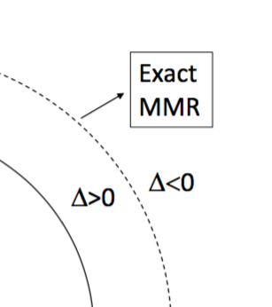
Figure 1: Sketch illustrating the meaning of $\Delta$: the solid line shows the position of the inner planet, and the dashed line the position of the outer planet when the system is at exact MMR, corresponding to $\Delta=0$. If the outer planet is interior (exterior) to the dashed line, $\Delta$ is positive (negative).

Using equations (25) and (26), we have:

$$\frac{d\Delta}{dt}= 3(q+1)\frac{n_{2}}{n_{1}}\left(e_{1}f_{1}\sin\phi_{1}+e_{2}f^{\prime}_{2}\sin\phi_{2}\right)\left[(q+1)n_{2}\frac{m_{1}}{m_{\star}}+qn_{1}\frac{\alpha m_{2}}{m_{\star}}\right]$$

$$+3(q+1)\frac{n_{2}}{n_{1}}\left(\frac{1}{2t_{a,2}}+\frac{e_{2}^{2}}{t_{e,2}}-\frac{1}{2t_{a,1}}-\frac{e_{1}^{2}}{t_{e,1}}\right).$$ (45)

Once again, we look for solutions with evolutionary long timescale, large compared to $t_{e,1}$ and $t_{e,2}$. We therefore can use equations (32) and (33) and combine them to express $\left(e_{1}f_{1}\sin\phi_{1}+e_{2}f^{\prime}_{2}\sin\phi_{2}\right)$ in terms of the eccentricities. Equation (45) then becomes:

$$\frac{d\Delta}{dt}= -3(q+1)\frac{n_{2}}{n_{1}}\left[(q+1)\frac{e_{1}^{2}}{t_{e,1}}\left(\frac{n_{2}}{n_{1}}\frac{m_{1}}{\alpha m_{2}}+1\right)+q\frac{e_{2}^{2}}{t_{e,2}}\left(\frac{n_{1}}{n_{2}}\frac{\alpha m_{2}}{m_{1}}+1\right)\right]$$

$$+\frac{n_{2}}{n_{1}}\frac{3(q+1)}{2}\left(\frac{1}{t_{a,2}}-\frac{1}{t_{a,1}}\right).$$ (46)

Here we assume that, although the planets may be moving away from MMR, the resonant angles are still librating around some fixed values, so that $\dot{\phi}_{1}=\dot{\phi}_{2}=0$. We have checked that this is indeed the case in all the numerical calculations we present below, even when departure from exact MMR is significant. This implies $\dot{\omega}_{1}=\dot{\omega}_{2}=\dot{\sigma}$. Using equations (20) and (21) and $\dot{\sigma}=(q+1)n_{2}-qn_{1}=n_{1}\Delta$, this yields:

$$e_{1}^{2}= \left(\frac{\alpha m_{2}}{m_{\star}}\right)^{2}\frac{f_{1}^{2}}{\Delta^{2}},$$ (47)

$$e_{2}^{2}= \left(\frac{m_{1}}{m_{\star}}\right)^{2}\left(\frac{n_{2}}{n_{1}}\right)^{2}\frac{f^{\prime 2}_{2}}{\Delta^{2}},$$ (48)

where we have replaced $\cos^{2}\phi_{1}$ and $\cos^{2}\phi_{2}$ by 1. Substituting into equation (46) and using $n_{2}/n_{1}=(\Delta+q)/(q+1)$, we finally obtain the following differential equation:

$$\Delta^{2}\frac{d\Delta}{dt}=-{\cal{A}}-{\cal{B}}\Delta^{2},$$ (49)

with:

$${\cal{A}}= \frac{3(\Delta+q)}{t_{e,1}}\left(\frac{\Delta+q}{q+1}\frac{m_{1}}{\alpha m_{2}}+1\right)\left(\frac{\alpha m_{2}}{m_{\star}}\right)^{2}\left[(q+1)f_{1}^{2}+\frac{q(\Delta+q)}{q+1}\frac{m_{1}}{\alpha m_{2}}f^{\prime 2}_{2}\frac{t_{e,1}}{t_{e,2}}\right],$$ (50)

$${\cal{B}}= \frac{3(\Delta+q)}{2t_{a,1}}\left(1-\frac{t_{a,1}}{t_{a,2}}\right).$$ (51)

As $\Delta+q=(q+1)n_{2}/n_{1}>0$, ${\cal{A}}$ is a positive definite function of $\Delta$.

We now discuss solutions of this equation in the case of both convergent and divergent migration, adopting a model where $t_{a,{\rm i}}$ and $t_{e,{\rm i}}$ are proportional to the semimajor axis (eq. [29] and [30]), which results from assuming that the disc surface mass density $\propto r^{-3/2}$.

3.3.1 Convergent migration:

In this regime, $t_{a,2}\leq t_{a,1}$, and ${\cal{B}}$ given by equation (51) is negative. Therefore equation (49) has equilibrium solutions with $\Delta$ constant such that $\Delta^{2}=-{\cal{A}}/{\cal{B}}$, where ${\cal{A}}$ and ${\cal{B}}$ are functions of $\Delta$.

Assuming small departure from resonance (which can be justified a posteriori), which implies $|\Delta|\ll q$ and therefore ${\cal{A}}$ and ${\cal{B}}$ independent of $\Delta$, ${\cal{A}}/{\cal{B}}$ can be expressed in terms of the masses and damping timescales. For convergent migration to occur, $m_{1}/m_{2}$ has to be on the order of unity or smaller. In that case, using $t_{a,1}/t_{e,1}\sim 10^{3}$ (eq. [29] and [30]), $\sqrt{-{\cal{A}}/{\cal{B}}}$ can be evaluated from equations (50) and (51) and is found to be very small compared to unity for Earth mass planets. Therefore, to a high degree of accuracy, the planets can be considered in exact MMR.

Equilibrium values of $\Delta$ can either be positive or negative, equal to $\pm\sqrt{-{\cal{A}}/{\cal{B}}}$. If $\Delta$ starts from an initial value exceeding the positive root of smallest magnitude, the right–hand side of equation (49) is positive, which implies that $d\Delta/dt>0$ and $\Delta$ moves away from this root. In the same way, $\Delta$ cannot converge toward the positive root from below. Convergence towards the negative root though is possible, both from below and from above, and therefore this is an equilibrium solution which can be approached time asymptotically. This corresponds to the formation and maintenance of a commensurability in which the planets are slightly further apart than at exact MMR.

If $\Delta$ is initially slightly larger than the positive root of smallest magnitude, as we have just pointed out, it diverges from it. In principle, there is the possibility of larger positive roots corresponding to equilibrium that could be approached time asymptotically if the migration timescales had an appropriate dependence on the orbital parameters. This is illustrated below in section 4.1.

3.3.2 Divergent migration: an approximate solution

We now consider the case where migration is divergent, which happens when $t_{a,2}>t_{a,1}$.

In that case, ${\cal{B}}$ given by equation (51) is a positive definite function of $\Delta$, and $\Delta$ given by equation (49) must decrease with time, corresponding to an expansion away from commensurability. There is no steady state in this case. The first term on the right–hand–side of equation (49) corresponds to expansion due to orbital circularization, and it dominates for small $\Delta$. The second term corresponds to divergent migration and it dominates for larger values of $\Delta$.

The solution of equation (49) is:

$$\Delta-\int_{0}^{\Delta}\frac{({\cal{A}}/{\cal{B}})d\Delta^{\prime}}{({\cal{A}}/{\cal{B}})+\Delta^{\prime 2}}=-\int_{0}^{t}{\cal{B}}(t^{\prime})dt^{\prime},$$ (52)

where we have assumed that $\Delta=0$ (exact commensurability) at $t=0$. Provided $\left|{\cal{A}}/{\cal{B}}\right|\ll 1$, most of the contribution to the integral on the left–hand–side comes from near $\Delta^{\prime}=0$. Therefore, when calculating this integral, we approximate ${\cal{A}}$, ${\cal{B}}$ and other orbital parameters by their value at the center of the resonance (i.e. at $\Delta=0$). Under these circumstances, ${\cal{A}}$ and ${\cal{B}}$ depend on orbital parameters through ${\cal{A}}\propto 1/t_{e,1}\propto 1/a_{1}$ and ${\cal{B}}\propto 1/t_{a,1}\propto 1/a_{1}$.

Equation (52) can then be written as:

$$\Delta-\sqrt{\frac{{\cal{A}}}{{\cal{B}}}}\tan^{-1}\left(\sqrt{\frac{{\cal{B}}}{{\cal{A}}}}\Delta\right)=-\int_{0}^{t}{\cal{B}}(t^{\prime})dt^{\prime}.$$ (53)

For small $t$ and hence $\Delta$, ${\cal{B}}(t^{\prime})$ on the right–hand side of this equation may in addition be assumed to be constant and equal to its value for $\Delta=0$ and $a_{1}=a_{1,0}$. Furthermore, we expand the left–hand–side in powers of $\Delta$, retaining only the first non vanishing term. This yields:

$$\Delta=-\left(3{\cal{A}}t\right)^{1/3}.$$ (54)

This time–dependence of $t^{1/3}$ is in agreement with previous results (Papaloizou & Terquem  2010, Lithwick & Wu 2012 and Batygin & Morbidelli 2013).

For larger values of $t$, ${\cal{B}}(t^{\prime})$ on the right–hand–side of equation (52) can no longer be assumed to be constant, whereas the $\tan^{-1}$ term becomes negligible compared to $\Delta$. We write ${\cal{B}}=({\cal{B}}a_{1})/a_{1}$, with the numerator being a constant. As the planets are moving away from MMR, $a_{1}$ is given by equation (43) and we can write:

$$\Delta=-\int_{0}^{t}{\cal{B}}(t^{\prime})dt^{\prime}=-\int_{0}^{t}\frac{{\cal{B}}t_{a,1}\;dt^{\prime}}{(a_{1,0}/a_{1})t_{a,1}-t^{\prime}}={\cal{B}}t_{a,1}\ln\left|1-\frac{a_{1}}{a_{1,0}}\frac{t}{t_{a,1}}\right|.$$ (55)

As this expression only becomes valid after some time that we note $t_{\rm ref}$, and at which $\Delta=\Delta_{\rm ref}$, we substract the form of equation (55) for $t=t_{\rm ref}$ from the form at time $t$, so that we finally obtain:

$$\Delta={\cal{B}}t_{a,1}\ln\left|\frac{1-\frac{a_{1}}{a_{1,0}}\frac{t}{t_{a,1}}}{1-\frac{a_{1}}{a_{1,0}}\frac{t_{\rm ref}}{t_{a,1}}}\right|+\Delta_{\rm ref}.$$ (56)

4 Numerical solutions

We solve equations (20)–(28) for the variables $\varpi_{1}$, $\varpi_{2}$, $\sigma$, $n_{1}$, $n_{2}$, $e_{1}$, $e_{2}$, $\phi_{1}$ and $\phi_{2}$. For illustrative purposes, we fix $q=2$, as the 3:2 MMR is common among observed systems.

4.1 Convergent migration

Convergent migration requires $t_{a,1}>t_{a,2}$ . From equation (29), this implies that $m_{2}/m_{1}>a_{2}/a_{1}=(1+1/q)^{2/3}=1.3$. We choose $m_{1}=1$ ${\rm M}_{\oplus}$ and $m_{2}=1.4$ ${\rm M}_{\oplus}$, which satisfies this condition. We adopt $H/r=0.02$, $m_{\rm d}=10^{-4}$ ${\rm M}_{\odot}$ and $m_{\star}=1$ ${\rm M}_{\odot}$. We start the inner planet at $a_{1}=2.5$ au and the outer planet at $a_{2}=a_{1}(1+1/q)^{2/3}=3.26$ au. The initial timescales are then, in years, $t_{e,1}=7.5\times 10^{2}$, $t_{a,1}=6.7\times 10^{5}$, $t_{e,2}=7\times 10^{2}$ and $t_{a,2}=6.3\times 10^{5}$. With these values, the criterion for permanent capture in resonance with finite libration amplitude, which is $m_{2}/m_{\star}>0.17(t_{e}/t_{a})^{3/2}q/(q+1)^{3/2}$, where $t_{e}$ and $t_{a}$ are typical eccentricity and semimajor axes damping timescales, is satisfied (Goldreich & Schlichting 2014). The initial values of $e_{1}$, $e_{2}$, $\varpi_{1}$, $\varpi_{2}$ and $\sigma$ are chosen arbitrarily as this does not affect the calculations.

Figure 2 shows the numerical results and a comparison with the analytical results. The semimajor axes decrease while maintaining commensurability, and their evolution is in excellent agreement with that given by equations (41) and (42). As expected, the resonant angles are close to 0^∘ or 180^∘, whereas the difference of the pericenter longitudes $\varpi_{1}-\varpi_{2}$ is close to $-180^{\circ}$. Both eccentricities reach equilibrium values which are also in excellent agreement with equations (36) and (35). The parameter $\Delta$ decreases slightly from the initial value of 0, and reaches the equilibrium solution $-\sqrt{-{\cal{A}}/{\cal{B}}}$, as predicted in section 3.3.1.

Figure 2: Evolution of the system for $q=2$, $m_{1}=1$ ${\rm M}_{\oplus}$ and $m_{2}=1.4$ ${\rm M}_{\oplus}$ (convergent migration) as a function of time (in years). The upper left–hand plot shows the semimajor axes (in au) corresponding to the numerical calculations (solid lines) and to the analytical results given by equations (41) and (42) (crosses). The upper right–hand plot shows the resonant angles $\phi_{1}$ and $\phi_{2}$ and the difference of the pericenter longitudes $\varpi_{1}-\varpi_{2}$ (in degrees). The lower left–hand plot shows the eccentricities corresponding to the numerical calculations (solid lines) and to the analytical results given by equations (36) and (35) (crosses). The lower right–hand plot shows $\Delta$ corresponding to the numerical calculations (solid line) and to the analytical result $-\sqrt{-{\cal{A}}/{\cal{B}}}$ with ${\cal{A}}$ and ${\cal{B}}$ given by equations (50) and (51) (crosses).

We have pointed out above that equilibrium solutions with $\Delta>0$, which correspond to the planets being interior to the MMR, could be attained if the migration timescales were adjusted appropriately. This is illustrated in figure 3. In this calculation, the planets start slightly interior to the 3:2 MMR, and the system is evolved with no migration but eccentricity damping timescales $t_{e,1}=t_{e,2}\simeq 4\times 10^{2}$ years. This produces an increase of the mean motions, with $n_{1}$ evolving faster than $n_{2}$ (see eq. [25] and [26]), so that the system evolves towards MMR. If the system kept evolving under the action of eccentricity damping only, it would pass through MMR and keep separating. However, before exact MMR is reached, we apply a convergent migration timescale about 100 times longer than that given by equation (29) which cancels out the expansion of the system, so that the planets stall interior to exact MMR for several $10^{7}$ years. This timescale could be increased by refining the migration timescale. As shown in figure 3, departure from exact MMR is significant. However, we have checked that the resonant angles still librate around 0^∘ and 180^∘ in that case, so that equations (20)–(28) can still be used to describe the evolution of the system. The situation we have described here is not very realistic but illustrates that equilibrium positions interior to MMR could be reached. Such a case could arise if, for example, movement towards MMR as a result of orbital circularization were balanced by very weak convergent migration.

Figure 3: Evolution of the system for the same parameters as in figure 2, except that here the timescales are adjusted in such a way that the planets stall interior to exact MMR. The plots show the ratio $n_{1}/n_{2}$ (upper plot) and $\Delta$ (lower plot) versus time (in years). The planets start slightly interior to the 3:2 MMR. The system is then evolved with no migration but eccentricity damping timescales $t_{e,1}=t_{e,2}\simeq 4\times 10^{2}$ years, so that the evolution is towards MMR. At $t=1.2\times 10^{7}$ years, before exact MMR is reached, a convergent migration timescale is applied which cancels out the expansion of the system. This results in the planets stalling interior to exact MMR for several $10^{7}$ years.

4.2 Divergent migration

Here we adopt $m_{1}=1$ ${\rm M}_{\oplus}$ and $m_{2}=1.3$ ${\rm M}_{\oplus}$ together with $m_{\rm d}=5\times 10^{-6}$ ${\rm M}_{\odot}$, which ensures that the planets move away from MMR on a long timescale, and we keep $m_{\star}=1$ ${\rm M}_{\odot}$ and $H/r=0.02$. The initial values of $a_{1}$ and $a_{2}$ are the same as above. Given that the planet masses are very close to the values they had in the convergent case above, but the disc mass is 20 times smaller, all the damping timescales are 20 times longer.

Figure 4 shows the evolution of $n_{1}/n_{2}$, of the semimajor axes and of $\Delta$ for this system. At the beginning of the evolution, $\Delta$ decreases as $t^{1/3}$, in agreement with equation (54), whereas at later times it evolves as predicted by equation (56).

We have checked that the eccentricities rapidly decrease to values very small compared to the equilibrium values, and that $\phi_{1}$ and $\phi_{2}$ keep librating around fixed values, even for such large departures from exact MMR, so that the analysis done in sections 3.2.2 and 3.3 applies.

Figure 4: Evolution of the system for $q=2$, $m_{1}=1$ ${\rm M}_{\oplus}$ and $m_{2}=1.3$ ${\rm M}_{\oplus}$ (divergent migration). The upper left–hand plot shows $n_{1}/n_{2}$ versus time (in years). The upper right–hand plot shows the semimajor axes (in au) versus time (in years). The solid lines correspond to the numerical calculations whereas the crosses correspond to the analytical results given by equation (43). The lower plots show $\Delta$ versus time (in years). The left–hand plot is a zoom on early times. The solid lines correspond to the numerical calculations whereas the crosses correspond to the analytical results given by equations (54) (left–hand plot) and (56) (right–hand plot).

5 Observed systems

Using the Open Exoplanet Catalogue, we have selected all the two planet systems in which the planet radii are smaller than 3.92 ${\rm R}_{\oplus}$ and the period ratio $P_{2}/P_{1}$ is smaller than 2.3. The constraint on the radius ensures that the planets are likely to be Earths or super–Earths and in the regime of type I migration. The constraint on the period ratio selects for systems which are close to MMR. There are 107 such systems. We have also included in our sample 9 systems with more than 2 planets but in which a pair of planets satisfies the above criteria and is far enough from the other planets that it is not expected to interact significantly with them.

5.1 Departure from exact resonances

The fact that $P_{2}/P_{1}\leq 2.3$ means that there exists an integer $q\geq 1$ such that $-0.25\leq P_{2}/P_{1}-(q+1)/q\leq 0.3$. Here we focus on first–order MMRs as these are the resonances in which low–mass planets are most easily captured (Papaloizou & Szuszkiewicz 2005). The first–order MMR the system is closest to is the (q+1):q resonance where $q$ is such that it minimizes $\left|P_{2}/P_{1}-(q+1)/q\right|$. The departure from exact resonance is then $\delta\equiv P_{2}/P_{1}-(q+1)/q$. However, according to this criterion, which we label (a), the system can either be interior ($\delta<0$) or exterior ($\delta>0$) to the resonance. As it has been argued that systems can more easily be produced exterior rather than interior to resonances, when $\delta<0$, we increase $q$ by 1, which makes $\delta>0$, as long as this change keeps $\delta<0.3$. This criterion is labelled (b). For example, $P_{2}/P_{1}=1.78$ corresponds to $q=1$ according to criterion (a), which gives $\delta=-0.22$. If we use criterion (b) instead, we have $q=2$ and $\delta=0.28$. Therefore the system can be seen as being either interior to the 2:1 MMR or exterior to the 3:2 MMR. The choice of 0.3 as a threshold for $\delta$ is completely arbitrary, but it has been taken large enough to favour systems exterior rather than interior to resonances, and small enough that the departure from exact MMR is within 15%.

Note that the relation between $\delta$ and $\Delta$ defined above is:

$$\Delta=\frac{-q\delta}{\delta+(q+1)/q}.$$ (57)

Figure 5 shows $\delta$ as a function of $q$ for all the systems in our sample, with $q$ chosen according to either criterion (a) or (b). (Similar plots have been published by Steffen & Hwang 2015, but without considering separately two–planet systems). Since the distance between MMR for $q\geq 2$ is less than $3/2-4/3\simeq 0.17$, all the systems with $P_{2}/P_{1}\leq 1.8$ can be seen as exterior to a MMR with $q\geq 2$ according to criterion (b). However, this is not true for $q=1$, and there are systems interior to the 2:1 resonance. Using criterion (a), there are 61 systems with $q=1$, 27 of them with $\delta<0$ and 34 with $\delta>0$. If we use criterion (b) instead, 3 of those systems with $\delta<0$ are assigned $q=2$ rather than $q=1$. Therefore, even if we adopt a criterion that favours planets being exterior rather than interior to MMR, we see that more than 40% of the systems close to the 2:1 resonance are interior to it.

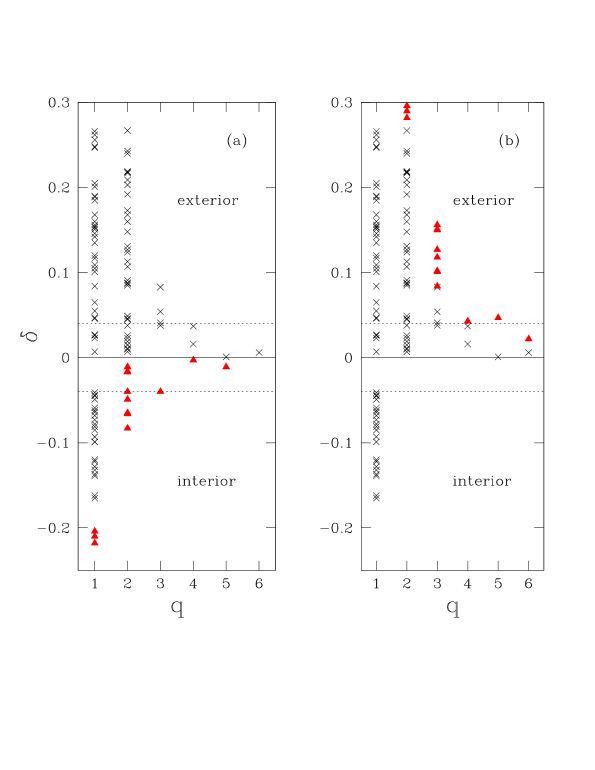
Figure 5: Departure from exact MMR, as measured by $\delta\equiv P_{2}/P_{1}-(q+1)/q$, versus $q$. For the left–hand plot, which is labelled (a), the value of $q$ is chosen in such a way as to minimize $\left|\delta\right|$. For the right–hand plot, which is labelled (b), the value of $q$ is chosen in such a way as to favour positive values of $\delta$ while keeping $\left|\delta\right|<0.3$. This amounts to increasing $q$ by 1 from the left to the right plots for some of the points, which are coloured in red. Exact MMR corresponds to $\delta=0$, whereas $\delta<0$ ($\delta>0$) corresponds to planets interior (exterior) to the resonance. The dashed lines represent $\delta=\pm 0.04$.

We see in figure 5 that when planets are very close to a resonance ($|\delta|<4\%$), they tend to be exterior rather than interior to the resonance, in agreement with Fabrycky et al. (2014). However, for even slightly larger departures, the spread is in either direction.

Labelling a system as exterior rather than interior to a resonance may seem like a semantic issue. However, it may be that the physical processes that move a system in one or the other direction from exact MMR are different. For example, it has been pointed out that dissipation of energy at constant angular momentum always moves the system further apart (Papaloizou & Terquem 2010, Papaloizou 2011, Lithwick & Wu 2012, Delisle et al. 2012, Batygin & Morbidelli 2013), so that it ends up being slightly exterior to the resonance. It is therefore of interest to try to understand whether the data indicate a tendency or not.

Figure 5 includes only first–order MMRs. As the 5:3 second–order MMR is located 0.33 below the 2:1 MMR, all the systems interior to the 2:1 resonance could be seen as being exterior to the 5:3 resonance. In figure 6, we again show $\delta$ as a function of $q$ but we now include the 5:3 MMR. We adopt criterion (b), which means that all the systems which had $q=1$ and $\delta<0$ are now assigned the 5:3 resonance, as are the systems which had $q=2$ and $\delta>0.167$.

Figure 6: Same as the right–hand plot of figure 5 but with the second–order 5:3 resonance now included. All the systems which had $q=1$ and $\delta<0$ are now assigned the 5:3 resonance, as are the systems which had $q=2$ and $\delta>0.167$.

Adding the 5:3 resonance enables to argue that all the systems are exterior to a resonance. However, this implies that the number of systems captured in the 5:3 MMR is comparable to that captured in the 3:2 MMR, which is not consistent with the result of numerical simulations for low–mass planets (Xiang–Gruess & Papaloizou 2015). Also, it forces us to consider that systems that are very close but interior to the 2:1 MMR are in fact captured in the 5:3 resonance and moved rather far away outside that resonance.

As has been pointed out in previous studies (Lissauer et al. 2011, Fabrycky et al. 2014), a striking feature of either figure 5 or figure 6 is that there is a large spread of $\delta$ around each MMR, even if we add the 5:3 resonance. From the figures above, we can conclude that either:

• all the systems attain exact MMR through smooth convergent migration; a few of them are subsequently moved exterior to the resonance by less than 4% or so by some ’gentle’ processes, while the majority of the systems are moved significantly away from the MMR in either direction by some other more efficient processes;

• only a small fraction of the systems attain exact MMR and are moved exterior to the resonance by less than 4% or so by some ’gentle’ processes; the vast majority of the systems are distributed randomly and were never captured in resonances.

In both scenarii, systems that would have found themselves slightly interior to a resonance by less than 4%, i.e. with $-0.04<\delta<0$, would be moved toward positive $\delta$ by the ’gentle’ process.

The ’gentle’ processes we refer to may involve dissipation of energy at constant angular momentum. More efficient processes that could take a system of two planets further away from resonance have been proposed but it is not clear so far that any of them can explain the range of data. This is investigated in more details in section 6 and discussed in section 7.

5.2 Convergent vs divergent migration

For most of the planets in our sample, a radius but not a mass has been measured. There is no unique relation between mass and radius for Earth and super–Earth like planets, as they span a wide range of compositions (Baraffe et al. 2014). However, some probabilistic mass–radius relations have been proposed based on a sample of well constrained planets (Wolfgang et al. 2016, Chen & Kipping 2017). In order to obtain a mass for the planets in our sample when there is no value derived from observations, we use the relations proposed by Chen & Kipping (2017):

$$\frac{m_{p}}{{\rm M}_{\oplus}} =0.952\left(\frac{r_{p}}{{\rm R}_{\oplus}}\right)^{3.584}\;\;\;{\rm for}\;r_{p}\leq 1.23\;{\rm R}_{\oplus},$$ (58)

$$\frac{m_{p}}{{\rm M}_{\oplus}} =1.407\left(\frac{r_{p}}{{\rm R}_{\oplus}}\right)^{1.698}\;\;\;{\rm for}\;r_{p}\geq 1.23\;{\rm R}_{\oplus},$$ (59)

where $m_{p}$ and $r_{p}$ are the mass and the radius of the planet. Comparing $m_{p}$ obtained from these relations with the observed value when it exists shows that these relations do not give very good individual fits. However, we note that in this paper we are more interested in the ratio of the masses than in the masses themselves, as it is the ratio that determines whether migration is convergent or divergent. Using either the observed mass when it exists of that derived using the relations above, together with equation (29), we calculate the ratio of the migration timescales that corresponds to the planets being in exact MMR:

$$\frac{t_{a,2}}{t_{a,1}}=\frac{m_{1}}{m_{2}}\frac{a_{2}}{a_{1}}=\frac{m_{1}}{m_{2}}\left(\frac{q+1}{q}\right)^{2/3},$$ (60)

where we have assumed that the eccentricities are very small compared to $H/r$. Convergent migration, which is required for the resonance to be maintained, corresponds to $t_{a,2}/t_{a,1}<1$.

Figure 7 shows $t_{a,2}/t_{a,1}$ as a function of $q$ for all the systems in our sample, with $q$ chosen according to criterion (a) (very similar plot would have been obtained by choosing criterion (b) instead). If the resonance were established and maintained during migration, then $t_{a,2}/t_{a,1}$ given by equation (60) would be smaller than 1. We see that this is not the case for 75 of the systems, which represents about 65% of the systems. Therefore, at least in the context of our disc model, and assuming constant planet masses, resonances for these systems have not been established during smooth migration.

Figure 7 also shows $t_{a,2}/t_{a,1}$ as a function of $\delta$ for all the systems in our sample, with $q$ chosen according to criterion (a) (again, very similar plot would have been obtained by choosing criterion (b) instead). We could have expected systems closer to resonances, i.e. with smaller values of $\delta$, to have preferentially $t_{a,2}/t_{a,1}<1$, which corresponds to convergent migration, but this is not the case. Including the 5:3 resonance would not change the conclusions of this subsection.

Figure 7: Ratio of the migration timescales $t_{a,2}/t_{a,1}$ versus $q$ (left–hand) and versus $\delta$ (right–hand). Here $q$ is chosen according to criterion (a), but very similar plots would have been obtained by choosing criterion (b) instead. Divergent (convergent) migration corresponds to $t_{a,2}/t_{a,1}>1$ ($t_{a,2}/t_{a,1}<1$). Only values of $t_{a,2}/t_{a,1}$ lower than 5 are displayed. We see that for about 65% of the systems, $t_{a,2}/t_{a,1}>1$, so that MMRs cannot have been established during smooth migration. Also, contrary to what could have been expected, there is no tendency for systems closer to resonance to have preferentially $t_{a,2}/t_{a,1}<1$.

6 Evolution of a resonant system entering a cavity

MMRs involving only two planets are very stable, which means that once established they are very difficult to disrupt. It has been proposed that chains of resonances could be disrupted when the disc dissipates, as then eccentricities grow (Izidoro et al. 2017). However, this is not the case for systems comprising two planets only in the mass regime we are investigating here. We have tested this hypothesis by solving the set of equations (20)–(28) and removing the disc adopting various timescales, but have found that in almost all cases the resonance survives.

It has been noted from previous simulations (eg. Xiang–Gruess & Papaloizou 2015) that significant increases in orbital eccentricities may occur when planets enter a cavity interior to the disc. This is potentially disruptive. However, the dynamics has not been studied in detail and is the focus of this section. This is important because pairs that originally had divergent migration in the smooth disc can form MMRs after the inner planet enters a cavity.

6.1 Disruption of the resonance when entering the cavity

Here we model the cavity as a discontinuity, meaning that the damping terms are discontinuously set to zero when the planet is located inside the inner edge. When the innermost planet enters the inner cavity, the resonance may be disrupted. This is illustrated in figure 8 for $q=1$. For fixed values of $m_{1}$, $m_{2}$ and $m_{d}$, this happens when the radius of the inner cavity, ${\rm r}_{\rm cav}$, is larger than some critical value ${\rm r}_{\rm crit}$. For a given $m_{1}$, ${\rm r}_{\rm crit}$ decreases when $m_{2}$ and $m_{d}$ increase. It can be seen on figure 8 that the eccentricity $e_{1}$ of the innermost planet reaches very high values after the planet enters the cavity, as there is no longer damping from the disc. This tends to disrupt the MMR. For a given MMR, the larger the cavity, the larger the separation between the planets, and the easier it is for the MMR to be disrupted when $e_{1}$ becomes large.

Figure 8: Evolution of the system for $q=1$, $m_{1}=1$ ${\rm M}_{\oplus}$, $m_{2}=1.6$ ${\rm M}_{\oplus}$, $m_{d}=3\times 10^{-5}$ ${\rm M}_{\odot}$ and ${\rm r}_{\rm cav}=0.3$ au as a function of time (in years). The upper left–hand plot shows the semimajor axes (in au). The upper right–hand plot shows $n_{1}/n_{2}$. The lower left–hand plot shows the resonant angles $\phi_{1}$ and $\phi_{2}$ and the difference of the pericenter longitudes $\varpi_{1}-\varpi_{2}$ (in degrees). The lower right–hand plot shows the eccentricities. The resonance is disrupted when the inner planet enters the cavity. Note that the calculations shown here cannot be trusted after the planet has entered the cavity, as the equations which are solved are only valid to first order in eccentricities. However, disruption of the resonance may be real.

The calculations shown in figure 8 have been done by solving the set of equations (20)–(28), which are only valid to first order in eccentricities and when the resonant angles librate. Therefore, although they may capture the disruption of the resonance, they cannot be used to follow the subsequent evolution of the system. In the next subsection, we solve the full equations to calculate the evolution of the system after the inner planet enters a cavity.

6.2 Settling into another resonance

Here, we solve the equations of motion for each planet:

$${{\rm d}^{2}{\boldsymbol{r}}_{\rm i}\over{\rm d}t^{2}}=-{Gm_{\star}\boldsymbol{r}_{\rm i}\over|\boldsymbol{r}_{\rm i}|^{3}}-{Gm_{\rm j}\left(\boldsymbol{r}_{\rm i}-\boldsymbol{r}_{\rm j}\right)\over|\boldsymbol{r}_{\rm i}-\boldsymbol{r}_{\rm j}|^{3}}-\sum_{k=1}^{2}{Gm_{\rm k}\boldsymbol{r}_{\rm k}\over|\boldsymbol{r}_{\rm k}|^{3}}+\boldsymbol{\Gamma}_{\rm i}\;,$$ (61)

where $\boldsymbol{r}_{\rm i}$ denotes the position vector of planet ${\rm i}$, and ${\rm j=2}$ or 1 for ${\rm i}=1$ or 2, respectively. The third term on the right–hand side is the acceleration of the coordinate system based on the central star (indirect term).

Acceleration due to tidal interaction with the disc is dealt with through the addition of extra forces as in Papaloizou & Larwood (2000, see also Terquem & Papaloizou 2007):

$$\boldsymbol{\Gamma}_{\rm i}=-\frac{1}{t_{m,{\rm i}}}\frac{{\rm d}\boldsymbol{r}_{\rm i}}{{\rm d}t}-\frac{2}{|\boldsymbol{r}_{\rm i}|^{2}t_{e,{\rm i}}}\left(\frac{{\rm d}\boldsymbol{r}_{\rm i}}{{\rm d}t}\cdot\boldsymbol{r}_{\rm i}\right)\boldsymbol{r}_{\rm i},$$ (62)

where $t_{m,{\rm i}}=2t_{a,{\rm i}}$ and $t_{e,{\rm i}}$ are the timescales on which the angular momentum and the eccentricity of planet ${\rm i}$ decrease. In the simulations presented below, $t_{m,{\rm i}}$ and $t_{e,{\rm i}}$ are given by equations (29) and (30), which means that the migration timescale in this subsection is half of what it was above. However this does not affect our conclusions. Equation (61) for each planet is solved using the $N$–body code described in Terquem & Papaloizou (2007). The evolution of the orbital eccentricities is accurately calculated by this code (see e.g., Teyssandier & Terquem 2014 for comparisons between analytical and numerical results), which is important here as eccentricities become very large.

Figure 9 shows the evolution of a system starting in the 2:1 MMR for $m_{1}=1$ ${\rm M}_{\oplus}$, $m_{2}=1.6$ ${\rm M}_{\oplus}$, $m_{d}=7\times 10^{-5}$ ${\rm M}_{\odot}$ and ${\rm r}_{\rm cav}=0.4$. After the inner planet enters the cavity, its eccentricity grows to large values and the system moves away from the 2:1 resonance. However, it quickly settles into the 3:2 MMR. We have checked that the resonant angles corresponding to the 3:2 MMR librate after that point. In all the runs we have performed starting with $q=1$, when the resonance is disrupted then the system moves into the 3:2 MMR. Note that in general the 2:1 resonance is rather weak, with the resonant angles having very large amplitude libration around fixed values. The 3:2 MMR is much more robust.

Figure 9: Evolution of the system for $q=1$, $m_{1}=1$ ${\rm M}_{\oplus}$, $m_{2}=1.6$ ${\rm M}_{\oplus}$, $m_{d}=7\times 10^{-5}$ ${\rm M}_{\odot}$ and ${\rm r}_{\rm cav}=0.4$ as a function of time (in years). The upper plot shows the eccentricity of the inner planet (solid line) and that of the outer planet (dashed line) in logarithmic scale. The lower plot shows $n_{1}/n_{2}$. The system starts in the 2:1 MMR. When the inner planet enters the cavity at time $t\simeq 6\times 10^{5}$ years, the resonance is disrupted. The system subsequently evolves into the 3:2 MMR.

Starting in exact 3:2 MMR, we have found in a number of cases that when the MMR is disrupted the system evolves towards $n_{1}/n_{2}\simeq 1.45$, which means a 5% departure from the initial 3:2 resonance. In that case, the resonant angles corresponding to the 3:2 MMR do not librate anymore, which indicates that the resonance has been disrupted, but this period ratio of 1.45 does not seem to correspond to another MMR. Therefore, there seems to be the possibility that the resonance is disrupted and the system moves interior to it, but only by a few percent. This is illustrated in figure 10. The fact the 4:3 MMR is not reached after the 3:2 resonance is disrupted is most likely due to the fact that the outer planet is not able to move over a distance large enough. As can be seen on figure 10, the final period ratio of 1.45 is attained more or less at the same time as when the eccentricities have stabilised, which happens when the interaction with the disc ceases. At that point, the semimajor axes are not evolving anymore. By contrast, in the case starting with the 2:1 MMR, the outer planet was able to move over a distance large enough that the 3:2 MMR could be reached. This is supported by the fact that, in that case, the final period ratio of 1.5 is attained before the eccentricities have stabilised.

Figure 10: Evolution of the system for $q=2$, $m_{1}=1$ ${\rm M}_{\oplus}$, $m_{2}=1.4$ ${\rm M}_{\oplus}$, $m_{d}=7\times 10^{-5}$ ${\rm M}_{\odot}$ and ${\rm r}_{\rm cav}=0.3$ as a function of time (in years). The upper plot shows the eccentricity of the inner planet (solid line) and that of the outer planet (dashed line) in logarithmic scale. The middle plot shows $n_{1}/n_{2}$. The lower plot shows the resonant angles corresponding to the 3:2 resonance. The system starts in the 3:2 MMR. When the inner planet enters the cavity at time $t\simeq 6\times 10^{5}$ years, the resonance is disrupted, as can been seen from the fact that the resonant angles stop librating. The system subsequently evolves towards $n_{1}/n_{2}=1.44$.

The large eccentricities obtained here when the inner planet enters the cavity may be produced in part by the fact that the damping timescales are set discontinuously to zero at the edge of the cavity. It is possible that a smoother transition would limit the growth of the eccentricities. However, the calculations above indicate that even with this extreme set up, the disruption of resonances does not lead to systems where the two planets are significantly distant from a resonance. Adopting a smoother transition is expected to be less disruptive and so would only reinforce this conclusion.

7 Discussion

In this section, we summarize our main results and discuss the implications of our study for planet formation.

7.1 Summary of the main results

In the first part of this paper, we have presented an analysis of a first–order $(q+1):q$ resonance for any $q\geq 1$ including migration torques. We have derived the values of the eccentricities and departure from exact resonance $\Delta$ at equilibrium in the case of convergent migration. We have also derived an expression for $\Delta$ as a function of time in the case of divergent migration. Such an expression had been obtained previously for small times $t$, where $|\Delta|\propto t^{1/3}$ (Papaloizou & Terquem  2010, Lithwick & Wu 2012, Batygin & Morbidelli 2013). We have extended the calculation to larger values of $t$ and incorporated the effect of migration torques which have not previously been considered, showing that in that regime $\Delta$ is a logarithmic function of $t$.

These analytical results have been found to be in good agreement with the results of the numerical integration of Lagrange’s planetary equations valid to first order in eccentricities in the vicinity of the resonance.

We have also shown that, under some circumstances, the planets could stall interior to exact resonance. This would happen for instance if the planets started interior to a resonance and with no migration but only eccentricity damping, as could be the case in parts of the disc with appropriate mass density variations. The system would then expand towards exact resonance, but the separation could become frozen before exact resonance is reached if the planets were resuming migration.

In the second part of the paper, we have discussed observations of two–planet systems which are close to a resonance. We have pointed out that departure from exact resonance is towards larger separations only if departures smaller than 4% are considered. For larger departures, which occur for most of the systems, there is no obvious preference for the offset to be in a particular direction.

Finally, we have investigated the evolution of a system in a resonance when the inner planet enters a cavity interior to the disc. We have found that the 2:1 MMR is easily disrupted, but the system quickly evolves toward the 3:2 resonance. The 3:2 MMR is more robust, although in some cases we have found that the period ratio decreases by a few percent while the resonance angles stop librating.

7.2 Migration versus in–situ formation

The analysis of the data suggests that even when a system is very close to MMR, the resonance in most cases cannot have been established while the planets were migrating smoothly through the disc. Therefore, if capture in resonance does occur, it is in general after the planets have reached the disc’s inner edge. That happens if one planet migrates first and penetrates inside a cavity interior to the disc, or stalls just beyond, and another planet subsequently migrates down towards the cavity and locks the inner planet into a resonance. This scenario can explain systems close to MMRs. However, if migration is a general outcome and happens in all the systems, since most systems show significant departure from exact MMR, there has to be a process capable of disrupting significantly the resonance after it is established in the way described above. Alternatively, there has to be a process that prevents the resonance from being established. Failing that, we have to conclude that the two planets have formed not too far away from the disc’s inner parts and that migration has been limited, in a scenario approximating in–situ formation.

Permanent capture into a resonance can be avoided for a range of parameters for which the resonance is overstable, as shown by Goldreich & Schlichting (2014). However, this requires the outer planet to be more massive than the inner one (Deck & Batygin 2015), which is in general not the case, as discussed above.

A number of processes capable of significantly moving systems away from resonances (by more than a few percent) have been proposed, but so far none of them seem to be able to single–handedly explain the data:

• turbulent fluctuations in the disc can destabilize resonances (Adams et al. 2008). It has been shown that, with an appropriate level of turbulence in the disc, stochastic migration is able to produce systems with orbital parameters which are in agreement with the data (Rein 2012). However, Batygin & Adams (2017) have recently argued that for any realistic parameters describing the disc, this process is only efficient if the total mass in the system if more than 3 ${\rm M}_{\oplus}$ which, given the uncertainty on the masses, makes it rather marginal though possibly not working for the largest masses.

• interaction between a planet and the wake of a companion produces significant departure from exact resonance (Baruteau & Papaloizou 2013). Note that this process does not necessarily require the MMR to be established through smooth convergent migration, although that was the case investigated by Baruteau & Papaloizou (2013). It would also work if the MMR were established with the inner planet near a cavity edge where the surface density decreased smoothly inwards, and in that case the outer planet may not have to be more massive. However, this process requires a particular relation between the planet masses and disc properties to work, so it is unlikely to be universal.

• departure from exact resonance may be significant if capture into resonance occurs during migration in a flared disc (Ramos et al. 2017). However, this would require convergent migration of all the systems near resonance, which is not consistent with the data.

• planets could move out of resonance after reaching the disc inner parts if the magnetospheric cavity expands and planets are trapped beyond the edge of the cavity and move outward with it (Liu et al. 2017). However, departure from resonance is induced only when the outer planet is more massive than the inner one, which is not generally the case, as shown above.

• resonances may be disrupted when the disc dissipates, as eccentricities get excited to high values (Izidoro et al. 2017). This requires more than two planets in the system (we have checked that resonances do survive disc dissipation for a broad range of parameters when only two planets are involved in the resonance) but, as inclinations are produced through this dynamical instability, transit observations may lead to only two planets being detected. However, even though the planets in the calculations of Izidoro et al. (2007) are significantly more massive than those in the Kepler sample, the fraction of stable resonant chains obtained in their model is significantly higher than that needed to match the distribution of observed planets.

• departures from resonance may happen after the gas in the disc dissipates and as a result of interactions between the planets and planetesimals (Chatterjee & Ford 2015). However, for significant departure to occur, the mass in the planetesimal disc has to be at least half the mass of the planets themselves. Such massive planetesimal populations would be unlikely in the inner parts of discs.

None of these processes taken in isolation can explain the range of observations, and it has yet to be shown whether when taken together they can reproduce the spread of period ratios which is observed. Strict in–situ formation of low mass planets has been investigated in previous studies. Hansen & Murray (2013) have shown that the output of their Monte Carlo model for the structure of low mass planets that form in–situ is in rather good agreement with Kepler observations, except for the fact that it does not produce enough single planet systems. Petrovich et al. (2013) have found using a simplified model that the distribution of period ratios for planets forming si–situ is similar to that observed by Kepler, which peaks around resonances. However, their model produces planets with final masses significantly exceeding those of super–Earths. Note that, in the in–situ formation scenario, for migration and resonant capture to be avoided, planets have to finish growing after most of the gas has been depleted.

Strict in–situ formation has not yet been shown convincingly to be able to explain the data. In addition, the existence of resonant chains indicates that some migration does occur. However, as shown in this paper, there is no support from the observations for extensive (over a large radial extent) convergent migration in a smooth disc. Only a small fraction of the systems have migrated through the disc and established a MMR (either during migration or after reaching the disc’s inner parts).

The above discussion suggests that there may be two populations of low mass planets:

• A small population where smooth migration was extensive so that MMRs were readily produced in the extended disc when it was convergent or near the cavity when it was not. In these systems, the planets have subsequently separated slightly, possibly due to tidal interaction with the star or other dissipative process. If we assume that all the systems in our sample with $0\leq\delta<0.04$ belong to this population, then the fraction of systems in this population is about 15%.

• Another larger population for which migration was much more modest, producing MMRs only in a small number of cases, this approximating in–situ formation.

Which scenario prevails may depend on the initial disc’s mass. Terquem (2017) pointed out that in low–mass discs, cores forming at around 1 au or beyond do not have enough time to migrate down to the disc’s inner parts. This is because the disc photoevaporates before migration of these cores can become significant. If systems close to the star and which have significant departure from MMRs have formed approximately in–situ, migration was not efficient in the disc in which they formed and therefore we would expect more low mass planets to be present further away.

Appendix A Coefficients in the disturbing function

In table 1, we give the values of the coefficients $f_{1}$ and $f_{2}$, calculated from equations (7) and (8), for $q$ between 1 and 6. Since $f_{2}^{\prime}\equiv f_{2}-2\alpha\delta_{q,1}$, we have $f_{2}^{\prime}=f_{2}-2^{1/3}$ for $q=1$ and $f_{2}^{\prime}=f_{2}$ for $q>1$.

$q$	$f_{1}$	$f_{2}$
1	$-1.190$	1.688
2	$-2.025$	2.484
3	$-2.840$	3.283
4	$-3.650$	4.084
5	$-4.456$	4.885
6	$-5.261$	5.686

Table 1: Numerical values of $f_{1}$ and $f_{2}$ for $q$ between 1 and 6.

References

- [2008] Adams, F. C., Laughlin, G., Bloch, A. M., 2008, ApJ, 683, 111
- [\citeauthoryearBaraffe et al.2014] Baraffe, I., Chabrier, G., Fortney, J., Sotin, C., 2014, Protostars and Planets VI, Eds H. Beuther, R. S. Klessen, C. P. Dullemond, T. Henning, Univ. of Arizona Press
- [2017] Batygin, K., Adams, F. C., 2017, Astron. J., 153, 120
- [2013] Batygin, K., Morbidelli, A., 2013, Astron. J., 145, 1
- [2013] Baruteau, C., Papaloizou, J. C. B., 2013, ApJ, 778, 7
- [\citeauthoryearChatterjee2013] Chatterjee, S., Ford, E. B., 2015, ApJ, 803, 33
- [2015] Deck, K. M., Batygin, K., 2015, ApJ, 810, 119
- [2017] Chen, J., Kipping, D., 2017, ApJ, 834, 17
- [2012] Delisle, J.-B., Laskar, J., Correia, A. C. M., Boué, G., 2012, A&A, 546, A71
- [2014] Fabrycky, D. C., et al., 2014, ApJ, 790, 146
- [\citeauthoryearGoldreich & Schlichting2014] Goldreich, P., Schlichting, H., 2014, Astron. J., 147, 32G
- [2017] Hands, T. O., Alexander, R. D., 2018, MNRAS, 474, 3998
- [2013] Hansen, B. M. S., Murray, N., 2013, ApJ, 775, 53
- [2017] Izidoro, A., Ogihara, M., Raymond, S. N., et al., 2017, MNRAS, 470, 1750
- [\citeauthoryearLissauer et al.2011] Lissauer, J., et al., 2011, ApJS, 197, 8
- [2017] Liu, B., Ormel, C. W., Lin, D. N. C., 2017, A&A, 601, 15
- [2012] Lithwick, Y., Wu, Y., 2012, ApJ, 756, L11
- [\citeauthoryearMurray & Dermott1999] Murray, C., Dermott, S., 1999, Solar System Dynamics, Cambridge University Press
- [2011] Papaloizou, J. C. B., 2011, CeMDA, 111, 83
- [2000] Papaloizou, J., Larwood, J., 2000, MNRAS, 315, 823
- [2015] Steffen, J. H., Hwang, J. A., 2015, MNRAS, 448, 1956 Papaloizou, J. C. B., Szuszkiewicz, E., 2005, MNRAS, 363, 153
- [2010] Papaloizou, J. C. B., Terquem, C., 2010, MNRAS, 405, 573
- [\citeauthoryearPetrovich et al.2013] Petrovich, C., Malhotra, R., Tremaine, S., 2013, ApJ, 770, 24
- [2012] Rein H., 2012, MNRAS, 422, 3611
- [2017] Ramos, X. S., Charalambous, C., Benítes–Llambay, P., Beaugé, C., 2017, A&A, 602, 101
- [2017] Terquem, C., 2017, MNRAS, 464, 924
- [2007] Terquem, C., Papaloizou J., 2007, ApJ, 654, 1110
- [2014] Teyssandier, J., Terquem, C., 2014, MNRAS, 443, 568
- [2016] Wolfgang, A., Rogers, L. A., Ford, E. B., 2016, ApJ, 825, 19
- [2015] Xiang–Gruess, M., Papaloizou, J. C. B., 2015, MNRAS, 449, 3043