Eigenenergies of excitonic giant-dipole states in cuprous oxide

Abstract

In this work we present the eigenspectra of a novel species of Wannier excitons when exposed to crossed electric and magnetic fields. In particular, we compute the eigenenergies of giant-dipole excitons in $\textrm{Cu}_{2}\textrm{O}$ in crossed fields. In our theoretical approach, we calculate the excitonic spectra within both an approximate as well as a numerically exact approach for arbitrary field configurations. We verify that stable bound excitonic giant-dipole states are only possible in the strong magnetic field limit, as this is the only regime providing sufficiently deep potential wells for their existence. Comparing both analytic as well as numerical calculations, we obtain excitonic giant-dipole spectra with level spacings in the range of $0.6\ldots 100\,\mu\textrm{eV}$.

I Introduction

In a semiconductor environment, excitons are the quanta of the fundamental optical excitation which consist of a negatively charged electron in the conduction band and a positively charged hole in the valence band [1; 2]. As the interaction between them can be modeled as a screened Coulomb interaction, excitons are often considered to be a solid-state quasi-particle analogue to the hydrogen atom [3; 4; 5]. In recent times, the measurement of hydrogen-like absorption spectrum of these quasi-particles up to principal quantum numbers of $n=25$ in cuprous oxide ($\textrm{Cu}_{2}\textrm{O}$) have attracted attention [6]. However, the hydrogen-like model of excitons is generally too simplistic, and has been expanded by taking into account the complex valence band structure and the cubic symmetry $O_{\rm h}$ of $\textrm{Cu}_{2}\textrm{O}$ [7; 8; 9; 10; 11; 12]. This ansatz has been both theoretically and experimentally successfully applied for describing the correct level structure due to fine- and hyperfine splitting of excitonic states [13].

The addition of external electric and magnetic fields further reduces the symmetry of the exciton states, thereby leading to level structures possessing numerous complex splittings of excitonic absorption lines [14; 15; 16]. For instance, high-resolution transmission spectroscopy of excitons in cuprous oxide subject to an external electric field increases the complexity of the measured spectra with increasing field strength. In particular, excitonic states with different parity become mixed, leading to optical activation of states which remain dark in zero external field [17; 18]. Furthermore, recent high-resolution spectroscopy and theoretical modeling of excitons in $\textrm{Cu}_{2}\textrm{O}$ have provided a fundamental understanding of complex absorption spectra in external magnetic fields for field strengths of up to $7\,\rm T$ and excitonic states with principal quantum numbers $n\leq 7$ [19; 20]. As the cubic lattice and the external magnetic field break all anti-unitary symmetries, several studies have shown that magneto-excitons in $\textrm{Cu}_{2}\textrm{O}$ obey GUE (Gaussian unitary ensemble) statistics [21; 22; 23].

In the case of field-dressed excitonic species, the total momentum of the system is not conserved, and an exact separation of the relative and center-of-mass degrees of freedom is impossible [24]. There exists, however, an alternative conserved quantity, the so-called pseudomomentum, with whose help one can carry out a pseudoseparation of the center-of-mass and relative motion for neutral systems. In a recently article, a theoretical description of field-dressed excitons in $\textrm{Cu}_{2}\textrm{O}$ has been developed [25]. There, it has been shown that the effect of the center-of-mass degrees of freedom on the internal motion is an effective potential that gives rise to a number of outer potential wells for certain values of the pseudomomentum and applied field strengths. Potentially bound states in these outer potential wells are of decentered character with an electron-hole separation of up to several micrometers, leading to huge permanent electric dipole moments, thereby justifying the label excitonic giant-dipole states. Its counterpart in atomic physics, i.e. atomic giant-dipole states, have been predicted theoretically [26; 27; 24; 28; 29; 30] and explored experimentally in the early 1990’s [31; 32].

Although the first study on excitonic giant-dipole potential surfaces has provided strong indications for the existence of excitonic giant-dipole states, a systematic analysis of their bound-state properties, such as binding energies and energy spectra, is still missing. In this work, we extend previous studies by deriving the irreducible tensor representation of field-dressed excitons, and calculating the eigenenergies of giant-dipole states in $\textrm{Cu}_{2}\textrm{O}$. Here, we employ both approximate as well as numerically exact approaches.

This paper is organized as follows. In Sec. II, we present the Hamiltonian of excitons in crossed electric and magnetic fields in its irreducible representation. Following this, in Sec. III.1, we analyze the possibility of bound excitonic giant-dipole states in the limit of strong electric fields. Within this regime, we perform an adiabatic approximation that provides us with the possibility to derive analytic results. We find that, in this limiting regime, no bound states are present due to insufficiently deep potential energy surfaces. Following the adiabatic approach, we perform a similar analysis for arbitrary electric and magnetic field strengths in Sec. III.2. We find that, in the strong magnetic field limit, the potential surfaces are sufficiently deep to provide bound states within the local potential minima. In Sec. IV, we finally consider full couplings between the potential surfaces and calculate the excitonic eigenspectra within an exact diagonalization approach for various field strengths and field orientations.

II The excitonic giant-dipole Hamiltonian

The Wannier excitons in $\textrm{Cu}_{2}\textrm{O}$ analyzed in this work are formed by an electron in the lowest $\Gamma^{+}_{6}$-conduction band and a positively charged hole in the uppermost (triply degenerate) $\Gamma^{+}_{5}$-valence band. The energy gap between the two bands is $E_{g}=2.17208\,\textrm{eV}$ [6]. In contrast to the conduction band, the three uppermost valence bands are deformed due to interband interactions and the non-spherical symmetry of the crystal. These properties can be represented by an effective $I=1$ quasi-spin representation in the hole degrees of freedom [11].

In crossed electric and magnetic fields, the excitonic system possesses a constant of motion, the so-called pseudomomentum $\hat{\boldsymbol{K}}$ with

$$\hat{\boldsymbol{K}}=\boldsymbol{P}-\frac{1}{2}\boldsymbol{B}\times\boldsymbol{r},\ \ \ \boldsymbol{r}=\boldsymbol{r}_{e}-\boldsymbol{r}_{h},$$ (1)

and eigenvalues $\boldsymbol{K}$ [33; 34; 35]. As it has been discussed in detail previously, the excitonic Hamiltonian $H_{\rm ex}$ can be transformed into a single-particle Hamiltonian [20; 25]

$$H_{\rm ex}=H_{0}+H_{\rm so}+H_{\rm B},$$ (2)

with

$$H_{0}=\frac{\boldsymbol{\pi}^{2}}{2m_{e}}+H_{h}(\boldsymbol{\pi})+V(\boldsymbol{r}),\ \ H_{\rm so}=\frac{2}{3}\bar{\Delta}(1+\boldsymbol{I}\cdot\boldsymbol{S}_{h}),$$ (3)

$$H_{\rm B}=\bar{\mu}_{B}[(3\kappa+\frac{g_{s}}{2})\boldsymbol{I}\cdot\boldsymbol{B}-g_{s}\boldsymbol{S}_{h}\cdot\boldsymbol{B}].$$

The first term in $H_{0}$ stems from the kinetic energy of the electron whose effective mass $m_{e}=0.985m_{0}$ is almost identical to the free electron mass $m_{0}$. The second term is the hole Hamiltonian

$$H_{h}(\boldsymbol{\pi}) = \frac{\boldsymbol{\pi}^{2}}{2m_{0}}(\gamma_{1}+4\gamma_{2})-\frac{3\gamma_{2}}{m_{0}}(\{\pi^{2}_{x}I^{2}_{x}\}+{\rm c.p.})$$ (4)

$$-\frac{6\gamma_{3}}{m_{0}}[\{\{\pi_{x}\pi_{y}\}\{I_{x}I_{y}\}\}+{\rm c.p.}]$$

which is more complex due to the three coupled valence bands. The material parameters $\gamma_{i},\ i=1,2,3$ are the so-called Luttinger parameter and characterize the considered material [37; 36]. The values for $\textrm{Cu}_{2}\textrm{O}$ are given in Appendix A. The mapping $\{ab\}=(ab+ba)/2$ is the symmetric product and c.p. denotes cyclic permutations [11].

The term $H_{\rm so}$ denotes the spin-orbit coupling of the hole-spin $\boldsymbol{S}_{h}$ with $\boldsymbol{I}$, while $H_{B}$ includes the coupling of the hole spins to the external magnetic field. As we do not include any kind of electronic spin-orbit coupling or spin-spin interaction, the electron spin $\boldsymbol{S}_{e}$ is not considered throughout this work. If not stated otherwise, we use excitonic Hartree units throughout this work, i.e. $e=\hbar=m_{0}/\gamma^{\prime}=1/4\pi\varepsilon_{0}\varepsilon=1$ (see Appendix A). Here, $\varepsilon=7.5$ is the static dielectric constant of the bulk material and $\gamma^{\prime}_{1}\equiv m_{0}/m_{e}+\gamma_{1}$.

The quantity $\boldsymbol{\pi}$ is a generalized kinetic momentum which contains, besides the configuration space degrees of freedom $\boldsymbol{p}$ and $\boldsymbol{r}$, the spin-1 matrices $I_{i},\ i=1,2,3$. In an arbitrary gauge, its components $\pi_{i}$ are given by [25]

$$\pi_{i}=1_{I}p_{i}-qA_{i}(\boldsymbol{r})+\partial_{i}f-\sum_{k}(\frac{m_{h}}{M}1_{I}\delta_{ki}-\Omega_{ki})\tilde{K}_{k}$$ (5)

with $M=m_{e}+m_{h}$ and

$$q=\frac{m_{e}-m_{h}}{M},\ \boldsymbol{A}(\boldsymbol{r})=\frac{1}{2}\boldsymbol{B}\times\boldsymbol{r},\ \tilde{\boldsymbol{K}}=\boldsymbol{K}+\boldsymbol{B}\times\boldsymbol{r},$$

where $m_{h}\equiv m_{0}/\gamma_{1}$ denotes the hole mass. As the function $f$ can be eliminated via a simple gauge transformation, it will no longer be considered. Together with the first term in Eq. (3), one can define a kinetic energy Hamiltonian

$$T(\boldsymbol{\pi})=\frac{\boldsymbol{\pi}^{2}}{2m_{e}}+H_{h}(\boldsymbol{\pi})$$ (6)

which parametrically depends on the pseudomomentum $\boldsymbol{K}$. The last term in $H_{0}$ represents a potential term $V$ that reads as

$$V(\boldsymbol{r}) = \left(\Omega_{1}\tilde{K}^{2}+\boldsymbol{E}\cdot\boldsymbol{r}-\frac{1}{r}\right)1_{I}-\Omega_{2}\sum_{i}\tilde{K}^{2}_{i}I_{ii}$$ (7)

$$-\frac{2}{3}\Omega_{3}\sum_{ij,j<i}\tilde{K}_{i}\tilde{K}_{j}I_{ij},\ \tilde{\boldsymbol{K}}=\boldsymbol{K}+\boldsymbol{B}\times\boldsymbol{r}.$$

It describes an effective two-body potential including the electron-hole Coulomb interaction, the Stark coupling, and magnetic field terms. Together with $H_{\rm so}$ and $H_{\rm B}$, it defines the exact electron-hole potential

$$V_{\rm gd}(\boldsymbol{r})=V(\boldsymbol{r})+H_{\rm so}+H_{\rm B}$$ (8)

for field-dressed excitons in cuprous oxide [25].

Using the vector components $\pi_{i}$ and $\tilde{K}_{i}$, one can define the symmetric and trace-free Cartesian tensor operators

$$I_{ij} = 3\{I_{i}I_{j}\}-2\delta_{ij},\ \ \Pi_{ij}=3\{\pi_{i}\pi_{j}\}-\boldsymbol{\pi}^{2}\delta_{ij},$$ (9)

$$\tilde{K}_{ij} = 3\tilde{K}_{i}\tilde{K}_{j}-\tilde{K}^{2}\delta_{ij},$$ (10)

$$\Xi_{ij} = \left(\Pi_{ij}+m_{0}(\frac{\Omega_{2}}{\gamma_{2}}\delta_{ij}+\frac{\Omega_{3}}{3\gamma_{3}}(1-\delta_{ij}))\tilde{K}_{ij}\right).$$ (11)

Using these tensor operators we derive the irreducible representation of the excitonic Hamiltonian given by Eq. (2), and we obtain

$$H_{\rm ex}=\frac{\boldsymbol{\pi}^{2}}{2}-\frac{\mu^{\prime}}{3}\{\Xi^{(2)}\cdot I^{(2)}\}+\frac{\delta^{\prime}}{3}\big{(}\sum_{k=\pm 4}\{[\Xi^{(2)}\times I^{(2)}]^{(4)}_{k}\}$$ (12)

$$+\frac{\sqrt{70}}{5}\{[\Xi^{(2)}\times I^{(2)}]^{(4)}_{0}\}\big{)}+\left(\Omega_{1}\tilde{K}^{2}+E^{(1)}\cdot r^{(1)}-\frac{1}{r}\right)$$

$$+H_{\rm so}+H_{\rm B}$$

with $\mu^{\prime}=(3\gamma_{3}+2\gamma_{2})/5\gamma^{{}^{\prime}}_{1}$ and $\delta^{{}^{\prime}}=(\gamma_{3}-\gamma_{2})/2\gamma^{{}^{\prime}}_{1}$. The mapping

$$\{[\Xi^{(2)}\times I^{(2)}]^{(4)}_{k}\}$$

$$\equiv\frac{1}{2}\left([\Xi^{(2)}\times I^{(2)}]^{(4)}_{k}+[I^{(2)}\times\Xi^{(2)}]^{(4)}_{k}\right)$$ (13)

reflects the fact that the Cartesian tensor components $\Xi_{ij}$ and $I_{kl}$ do not necessarily commute. We note that this Hamiltonian is the most compact irreducible tensor representation of excitons in external electric and magnetic fields for arbitrary field strengths and field directions. Obviously, one can derive irreducible representations for kinetic and potential energy terms separately. These can be found in Appendix C.

III Adiabatic approximation

As it has been shown in Ref. [25], the diagonalization of the giant-dipole potential $V_{\rm gd}$ provides six distinct potential energy surfaces with energetic separations in the range of a few hundred $\mu\textrm{eV}$ up to $100\,\textrm{meV}$. In Fig. 1, we show typical potential curves for field strengths $B=1\,\textrm{T}$ and $E=1\,\textrm{kV/cm}$. One clearly observes local potential minima at distances several micrometers away from the Coulomb center. For each potential surface, we obtain the corresponding eigenvector $|\phi_{i}(\boldsymbol{r})\rangle,\ i=1,...,6$ including their spatial dependence on the electron-hole separation $\boldsymbol{r}$.

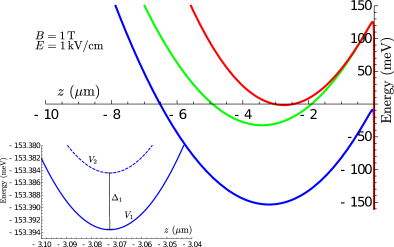
Figure 1: Potential curves for $B=1\,\rm T$, $E=1\,\rm kV/cm$. The specific field configurations are $\boldsymbol{B}||[100]$ and $\boldsymbol{E}||[001]$. The inset shows the adjacent potential curves $V_{1}$ and $V_{2}$ where the spacing $\Delta_{1}$ is indicated as well.

We can define the following quantities that characterize the individual giant-dipole potential curves:

• the potential depth $V^{(\alpha)}_{\rm d}$ given by

  $$V^{(\alpha)}_{\rm d}=\lim_{x\rightarrow\infty}\ V_{\alpha}(x,0,z^{(\alpha)}_{\rm min})-V_{\alpha}(\boldsymbol{r}^{(\alpha)}_{\rm min}),$$

• the quantity $\Delta_{\alpha}$ defining the energetic separation between two adjacent potential surface, i.e.

  $$\Delta_{\alpha}=V_{\alpha+1}(\boldsymbol{r}^{(\alpha+1)}_{\rm min})-V_{\alpha}(\boldsymbol{r}^{(\alpha)}_{\rm min}).$$

We emphasize that all six potential surfaces possess local minima. This is in contrast to previous work [25], where only four out of six surfaces possessed minima, which results from a different choice of Luttinger parameters which were only published recently [19]. Indeed, the potential surfaces’ topologies sensitively depend on the specific values of the Luttinger parameters [37; 36]. For this reason, a precise determination of excitonic giant-dipole properties such as level spacings and binding energies might provide the possibility of determining the specific Luttinger parameters with a higher degree of accuracy.

Although the giant-dipole potential is diagonal within this basis, the set $\{|\phi_{i}(\boldsymbol{r})\rangle_{i=1,...,6}\}$ is not suitable to diagonalize the total excitonic Hamiltonian $H_{\rm ex}$ as the kinetic part of Eq. (2) does not commute with the potential. More precisely, the coupling between different eigenstates $|\phi_{i}(\boldsymbol{r})\rangle$ generated by the kinetic energy operator induces transitions between the potential energy surfaces $V_{i}(\boldsymbol{r})$. This feature is well-known in molecular physics where these kinds of non-adiabatic transitions between electronic eigenstates are induced by the kinetic energy of the nuclei [38].

In a first ansatz, we follow the adiabatic approach from molecular physics by neglecting all excitonic transitions between a set of different potential surfaces. In particular, we define effective Hamiltonians

$$H^{(\alpha)}_{\rm eff}\equiv\langle\phi_{\alpha}(\boldsymbol{r})|H_{\rm ex}|\phi_{\alpha}(\boldsymbol{r})\rangle_{\rm spin},\ \alpha=1,...,6$$ (14)

by introducing

$$I^{(\alpha)}_{i}(\boldsymbol{r}) \equiv \langle\phi_{\alpha}(\boldsymbol{r})|I_{i}|\phi_{\alpha}(\boldsymbol{r})\rangle_{\rm spin},\ \ i=x,y,z,$$ (15)

$$\langle\Omega_{ki}\rangle_{\alpha}(\boldsymbol{r}) \equiv \langle\phi_{\alpha}(\boldsymbol{r})|\Omega_{ki}|\phi_{\alpha}(\boldsymbol{r})\rangle_{\rm spin},$$ (16)

$$\pi^{(\alpha)}_{i}(\boldsymbol{r}) \equiv \langle\phi_{\alpha}(\boldsymbol{r})|\pi_{i}|\phi_{\alpha}(\boldsymbol{r})\rangle_{\rm spin}.$$ (17)

In these expressions, the expectation values $\langle...\rangle_{\rm spin}$ are only computed with respect to the spin-1 and spin-1/2 degrees of freedom $\boldsymbol{I}$ and $\boldsymbol{S}_{h}$, respectively. This means that the effective quantities $H^{(\alpha)}_{\rm eff}$ and $I^{(\alpha)}_{i}(\boldsymbol{r})$ are functions of the canonical conjugated variables $\boldsymbol{p}$ and $\boldsymbol{r}$, respectively. In particular, the components $\pi_{i}$ of the kinetic momentum are now given by

$$\pi^{(\alpha)}_{i}=p_{i}-qA^{(\alpha)}_{i}(\boldsymbol{r})$$ (18)

with

$$A^{(\alpha)}_{i}=A_{i}(\boldsymbol{r})+g^{(\alpha)}_{i}(\boldsymbol{r})$$ (19)

and

$$g^{(\alpha)}_{i}(\boldsymbol{r})=\frac{1}{q}\sum_{k}\left(\frac{m_{h}}{M}\delta_{ki}-\langle\Omega_{ki}\rangle_{\alpha}\right)\tilde{K}_{k}.$$ (20)

Obviously, in the adiabatic approximation the homogeneous magnetic field is replaced by a spatially dependent field that can be computed from

$$\boldsymbol{B}^{(\alpha)}(\boldsymbol{r})=\boldsymbol{\nabla}\times\boldsymbol{A}^{(\alpha)}(\boldsymbol{r}).$$ (21)

By defining spatially dependent Luttinger parameters

$$\gamma^{(\alpha)}_{2,i}\equiv\gamma_{2}I^{(\alpha)2}_{i}(\boldsymbol{r}),\ \ \gamma^{(\alpha)}_{3,ij}\equiv\gamma_{3}I^{(\alpha)}_{i}(\boldsymbol{r})I^{(\alpha)}_{j}(\boldsymbol{r}),$$ (22)

we can write the effective Hamiltonians $H^{(\alpha)}_{\rm eff}$ as

$$H^{(\alpha)}_{\rm eff} = \frac{\boldsymbol{\pi}^{2}}{2\mu}-\frac{3}{\gamma^{\prime}_{1}}\left(\gamma^{(\alpha)}_{2,x}(\boldsymbol{r})\pi^{(\alpha)2}_{x}+\textrm{c.p.}\right)$$ (23)

$$-\frac{6}{\gamma^{\prime}_{1}}\left(\gamma^{(\alpha)}_{3,xy}(\boldsymbol{r})\pi^{(\alpha)}_{x}\pi^{(\alpha)}_{y}+\textrm{c.p.}\right)+V^{(\alpha)}_{\rm gd}(\boldsymbol{r})$$

with $\mu^{-1}=1+4\gamma_{2}/\gamma^{\prime}_{1}$ [see Eq. (14)].

III.1 Strong electric-field limit

Before we analyze the excitonic system in adiabatic approximation, we consider the limit of strong electric fields. In this limit, one can neglect the spin-orbit coupling $H_{\rm so}$ as well as the magnetic field coupling $H_{B}$. In this approximation, the excitonic Hamiltonian reduces to the direct sum $H_{\rm ex}=H_{0}\oplus 1_{s=1/2}$. Hence, the problem of determining the excitonic giant-dipole states is equivalent to the eigenvalue problem of a $3\times 3$-matrix, which can be solved analytically for arbitrary electric and magnetic field configurations. However, as it has been shown in Ref. [25], for a magnetic field oriented along the $[100]$ and an electric field in the $[001]$ direction, the expressions for the potential energy surfaces $V_{i}(\boldsymbol{r})$ and eigenstates $|\phi_{i}(\boldsymbol{r})\rangle$ are more compact and given by

$$V_{1}(\boldsymbol{r}) = \left(\Omega_{1}-\Omega_{2}\right)\tilde{K}^{2}+Ez-\frac{1}{r},$$

$$V_{2,3}(\boldsymbol{r}) = \left(\Omega_{1}-\Omega_{2}\right)\tilde{K}^{2}+Ez-\frac{1}{r}+\frac{3}{2}\Omega_{2}\left(\tilde{K}^{2}_{2}+\tilde{K}^{2}_{3}\right)$$ (24)

$$\pm\frac{1}{2}\sqrt{9\Omega^{2}_{2}\left(\tilde{K}^{2}_{2}-\tilde{K}^{2}_{3}\right)^{2}+4\Omega^{2}_{3}\tilde{K}^{2}_{2}\tilde{K}^{2}_{3}},$$

and

$$|\phi_{1}(\boldsymbol{r})\rangle = |1\rangle,$$

$$|\phi_{2}(\boldsymbol{r})\rangle = \cos(\gamma)|2\rangle-\sin(\gamma)|3\rangle,$$

$$|\phi_{3}(\boldsymbol{r})\rangle = \sin(\gamma)|2\rangle+\cos(\gamma)|3\rangle$$ (25)

where the mixing angle $\gamma(\boldsymbol{r})$ is defined as

$$\tan(2\gamma)=\frac{2\Omega_{3}\tilde{K}_{2}\tilde{K}_{3}}{3\Omega_{2}(\tilde{K}^{2}_{2}-\tilde{K}^{2}_{3})}.$$ (26)

Interestingly, the mixing angle does not depend on the external electric field. In case that also $\boldsymbol{K}=0$, even the dependence on the magnetic field cancels out. If we calculate the quantities from Eq. (17) in the strong electric field limit, we obtain

$$I^{(\alpha)}_{i}(\boldsymbol{r})=0,\ \ \langle\Omega_{ki}\rangle_{\alpha} = (C_{1}-\frac{2}{3}C_{2})\delta_{ki}$$

and

$$\pi_{i}=p_{i}-q\tilde{A}^{(i)}_{\rm sym}(\boldsymbol{r})-\frac{\tilde{m}_{h}}{M}\tilde{K}_{i},$$ (27)

with

$$\tilde{m}_{h}=m_{h}-M(C_{1}-\frac{2}{3}C_{2})$$ (28)

and

$$\tilde{A}^{(i)}_{\rm sym}(\boldsymbol{r})=\frac{1}{2}\tilde{\boldsymbol{B}}\times\boldsymbol{r},\ \ \ \tilde{\boldsymbol{B}}=\left(1+2\frac{\tilde{m}_{h}}{qM}\right)\boldsymbol{B}.$$ (29)

The $\tilde{K}$-dependent term in Eq. (27) can be written as $\partial_{i}\tilde{K}_{i}x_{i}$, i.e. it can be eliminated by a simple gauge transformation. In addition, the giant-dipole Hamiltonian is determined by an effective magnetic field $\tilde{\boldsymbol{B}}$ that is parallel to the initial $B$-field, but possesses a different magnitude $\tilde{B}$ with $\tilde{B}/B=1+2\tilde{m}_{h}/qM\approx 1.6$, which is an enhancement of around $60\%$. We note that both quantities $\tilde{m}_{h}$ and $\boldsymbol{\tilde{B}}$ do not depend on the specific potential surface.

We finally obtain in the strong electric field approximation the following excitonic Hamiltonian

$$H^{(\alpha)}_{\rm eff}=\frac{\boldsymbol{\pi}^{2}}{2\mu}+V_{\alpha}(\boldsymbol{r}),$$ (30)

whereby the potentials $V_{\alpha}$ are given by Eq. (24). The set of effective excitonic Hamiltonians $H^{(\alpha)}_{\rm eff}$ is identical to the Hamiltonian discussed previously [25]. There it has been shown that the giant-dipole potential surfaces $V_{\alpha}(\boldsymbol{r})$ possess minima at $\boldsymbol{r}_{\rm min}=(0,0,z_{\rm min})$ with

$$z^{(1,2)}_{\rm min} = \frac{E}{6(\Omega_{1}+\frac{1}{2}(1\pm 3)\Omega_{2})B^{2}}[2\cos(\frac{\theta+2\pi}{3})-1]$$

and $\cos(\theta)=54(\Omega_{1}+\frac{1}{2}(1\pm 3)\Omega_{2})^{2}B^{4}/E^{3}-1$. Although Eq. (30) is very similar to the atomic Hamiltonian discussed in Ref. [28], we stress that in the present case the potential $V_{\alpha}(\boldsymbol{r})$ is determined by the bare external magnetic field $\boldsymbol{B}$, while the kinetic energy term in Eq. (30) depends on the effective field $\tilde{\boldsymbol{B}}$.

In order to obtain the energies and wave functions of the excitonic giant-dipole species, we expand the potential surfaces around their local minima. Including terms up to second order, we find the harmonically approximated potentials

$$V^{(\alpha)}_{\rm h}(\boldsymbol{r})=\frac{\mu}{2}\omega^{(\alpha)}_{x}x^{2}+\frac{\mu}{2}\omega^{(\alpha)}_{y}y^{2}+\frac{\mu}{2}\omega^{(\alpha)}_{z}z^{2}$$ (31)

with the frequencies

$$\omega^{(\alpha)}_{x} = \sqrt{-\frac{1}{\mu z^{(\alpha)3}_{\rm min}}},\ \ \alpha=1,2,3\ \ ,$$

$$\omega^{(1)}_{y} = \omega^{(3)}_{y}=\sqrt{\frac{1}{\mu}\left(2(\Omega_{1}-\Omega_{2})B^{2}-\frac{1}{z^{(1)3}_{\rm min}}\right)},$$

$$\omega^{(2)}_{y} = \sqrt{\frac{1}{\mu}\left(2(\Omega_{1}+2\Omega_{2})B^{2}-\frac{1}{z^{(2)3}_{\rm min}}\right)},$$

$$\omega^{(1)}_{z} = \omega^{(3)}_{z}=\sqrt{\frac{2}{\mu}\left((\Omega_{1}-\Omega_{2})B^{2}+\frac{1}{z^{(1)3}_{\rm min}}\right)},$$

$$\omega^{(2)}_{z} = \sqrt{\frac{2}{\mu}\left((\Omega_{1}+2\Omega_{2})B^{2}+\frac{1}{z^{(2)3}_{\rm min}}\right)}.$$ (32)

As it has been discussed in Ref. [25], the eigenenergies and eigenstates can be obtained analytically via a unitary transformation which decouples the $(y,z)$-degrees of freedom leading to a set of three decoupled harmonic oscillators. Apart from the frequencies $\omega^{(\alpha)}_{z}$, the remaining energy spacings are equidistant with frequencies

$$\omega^{(\alpha)}_{1,2} = \frac{1}{\sqrt{2}}[\omega^{(\alpha)2}_{z}+\omega^{(\alpha)2}_{y}+\omega^{2}_{c}$$

$$\pm\sqrt{(\omega^{(\alpha)2}_{z}+\omega^{(\alpha)2}_{y}+\omega^{2}_{c})^{2}-4\omega^{(\alpha)2}_{z}\omega^{(\alpha)2}_{y}}]^{1/2}$$

and $\omega_{c}=q\tilde{B}/\mu$.

Although the excitonic eigenenergies and eigenstates are given analytically, one has to remember that these results have been derived within an harmonic approximation in the vicinity of the outer potential well. However, the exact potential surfaces possess an ionization limit in the direction of the external magnetic field. For this reason, one has to ensure that for a certain field configuration the calculated ground state still lies deep within the outer potential well. To analyze this issue in more detail we define the quantity

$$\eta^{(\alpha)} \equiv \frac{V^{(\alpha)}_{\rm d}-(\varepsilon_{000}-V_{\rm min})}{V^{(\alpha)}_{\rm d}}$$ (33)

$$= 1-\frac{|z^{(\alpha)}_{\rm min}|(\omega^{(\alpha)}_{x}+\omega^{(\alpha)}_{1}+\omega^{(\alpha)}_{2})}{2},$$

which accounts for the energy difference between the potential depth $V^{(\alpha)}_{\rm d}$ and the spacing between the ground state and the potential minimum, i.e. $\varepsilon_{000}-V_{\rm min}$. In Fig. 2, we show the quantity $\eta^{(1)}$ for electric and magnetic fields of $1\,\textrm{kV/cm}\leq E\leq 3\,\textrm{kV/cm}$ and $1\,\textrm{T}\leq B\leq 2\,\textrm{T}$, respectively.

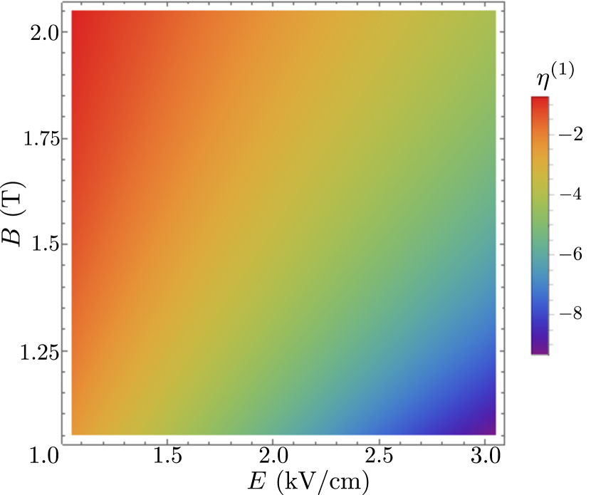
Figure 2: Density plot of $\eta^{(1)}$ for $1\,\textrm{kV/cm}\leq E\leq 3\,\rm kV/cm$ and $1\,\rm{T}\leq B\leq 2\,\rm T$. We see that in this strong-field limit we have $\eta^{(1)}<0$, i.e. no bound states are found in this regime.

One observes that in the considered field strength regime $\eta^{(1)}<0$, which means that the giant-dipole ground state lies above the ionization limit of the potential surface. The same result are obtained for the remaining potential surfaces, i.e. $\eta^{(2,3)}<0$. As a consequence, we expect no bound excitonic giant-dipole states in the limit of strong electric fields.

III.2 Arbitrary field strengths

In a next step, we keep the adiabatic approximation but leave the limit of strong electric fields in order to analyze arbitrary field strengths. Again, we consider $\boldsymbol{B}||[100]$ and $\boldsymbol{E}||[001]$. In this case, a rigorous analysis is rather complicated as the adiabatic Hamiltonians $H^{(\alpha)}_{\rm eff}$ do not only depend on spatially varying magnetic fields, but also on spatially dependent Luttinger parameters defined in Eq. (22). However, we may employ the fact that we are mainly interested in the bound states localized around the minima of the outer potential wells. For this reason, we make use of the approximation that the eigenstates do not strongly vary in the vicinity of a certain potential minimum. To illustrate that in more detail, we go back to the strong-field limit discussed in the previous section. According to Eq. (25), the spatial dependence of the eigenvectors are given by the mixing angle $\gamma$ determined by Eq. (26). If we consider $K=0$, we directly see that $\gamma(\boldsymbol{r}_{\rm min})=0$, which gives

$$|\phi_{1}(\boldsymbol{r}_{\rm min})\rangle = |1\rangle,$$

$$|\phi_{2}(\boldsymbol{r}_{\rm min})\rangle = |2\rangle,$$

$$|\phi_{3}(\boldsymbol{r}_{\rm min})\rangle = |3\rangle.$$ (34)

Obviously, the eigenstate $|\phi_{1}(\boldsymbol{r})\rangle=|\phi_{1}(\boldsymbol{r}_{\rm min})=|1\rangle\ \forall\ \boldsymbol{r}\in\mathbb{R}^{3}$. To analyze the deviation of the remaining eigenstates from the corresponding eigenstates at the minimum positions, we need to look at the spatial dependence of $\cos(\gamma(\boldsymbol{r}))$ in more detail.

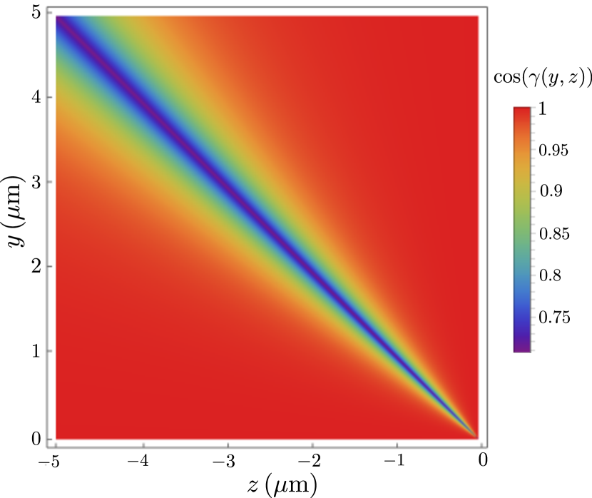
Figure 3: Density plot of $\cos(\gamma(y,z))$ for applied field strengths of $E=1\,\textrm{kV/cm}$ and $B=1\,\textrm{T}$. In the vicinity of the potential minima $z\approx-3\,\mu\textrm{m}$, one finds $\cos(\gamma(y,z))\approx 1$, which means that the corresponding eigenvectors only minor differ from the eigenstate at the potential minimum.

In Fig. 3, we show the mixing angle $\cos(\gamma(y,z))$ for applied field strengths $B=1\,\textrm{T}$ and $E=1\,\textrm{kV/cm}$ in the spatial range $0\leq y\leq 5\,\mu\rm m$ and $-5\,\mu\textrm{m}\leq z\leq 0$. For these field strengths, the potential minima are located at $z^{(1)}_{\rm min}=-3.07\,\mu\textrm{m}$, $z^{(3)}_{\rm min}=-3.25\,\mu\textrm{m}$ and $z^{(5)}_{\rm min}=-2.8\,\mu\textrm{m}$, respectively. We see that, in the vicinity of the potential minima $(z\approx 3\,\mu\textrm{m})$, $\cos(\gamma)$ remains close to unity, which means that the deviations from the pure eigenstates close to the minimum positions remain negligible. This result is not only valid for strong electric fields, but also for all field strengths considered throughout this work. This means that for the calculation of the matrix elements of the kinetic energy we can use the eigenvectors at the minimum position, i.e. $I^{(\alpha)}_{i}(\boldsymbol{r})\rightarrow I^{(\alpha)}_{i}(\boldsymbol{r}_{\rm min})$.

Analogous to the strong electric-field limit, we now define a renormalized vector potential using Eq. (17), from which the effective magnetic field $\boldsymbol{\tilde{B}}^{(\alpha)}$ is obtained as $\boldsymbol{\tilde{B}}^{(\alpha)}=\boldsymbol{\nabla}\times\boldsymbol{\tilde{A}}^{(\alpha)}$. However, it turns out that

$$\sum_{k}\langle\Omega_{ki}\rangle_{\alpha}\approx\langle\Omega_{ii}\rangle_{\alpha},$$ (35)

which means that the components $\tilde{B}^{(\alpha)}_{i}$ of the effective magnetic field are given by

$$\tilde{B}^{(\alpha)}_{i}=\left[1+\frac{2}{q}\left(\frac{m_{h}}{M}-\langle\Omega_{ii}\rangle_{\alpha}\right)\right]B_{i}.$$ (36)

The magnetic field $\boldsymbol{\tilde{B}}^{(\alpha)}$ is, in general, no longer parallel to the incident field $\boldsymbol{B}$ as it now points into the direction of the unit vector

$$\boldsymbol{e}^{(\alpha)}_{\tilde{\boldsymbol{B}}}=\frac{1}{|\tilde{\boldsymbol{B}}^{(\alpha)}|}(\tilde{B}^{(\alpha)}_{1},\tilde{B}^{(\alpha)}_{2},\tilde{B}^{(\alpha)}_{3})^{T},$$ (37)

with the magnitude $|\tilde{\boldsymbol{B}}^{(\alpha)}|=\sqrt{\tilde{B}^{(\alpha)2}_{1}+\tilde{B}^{(\alpha)2}_{2}+\tilde{B}^{(\alpha)2}_{3}}$. In contrast to the strong electric-field limit discussed in Sec. III.1, the effective magnetic field now depends on the specific potential curve under consideration via the matrix elements of the $\Omega_{ii}$-matrices.

In Fig. 4, we show $\tilde{B}^{(1)}_{1}/B$ as a function of the external field parameters for applied field strengths in the range of $1\,\textrm{T}\leq B\leq 4\,\textrm{T}$ and $1\,\textrm{kV/cm}\leq E\leq 4\,\textrm{kV/cm}$. In contrast to the approximation discussed in Sec. III.1 we now find that, depending on the specific field strengths, not only positive-valued effective magnetic field strengths, but also fields with negative values. In particular, for strong external magnetic fields one finds $\tilde{B}^{(1)}_{1}<0$, which means that not only the magnitude of the magnetic field is modified but also its direction with respect to the external field is changed. However, for sufficiently strong electric fields the sign of the magnetic field becomes positive and reaches a maximum value of around $1.5B$. As expected, this is quite close to the effective $B$-field $\tilde{B}=1.6B$ obtained in the strong electric-field approximation derived in Eq. (29).

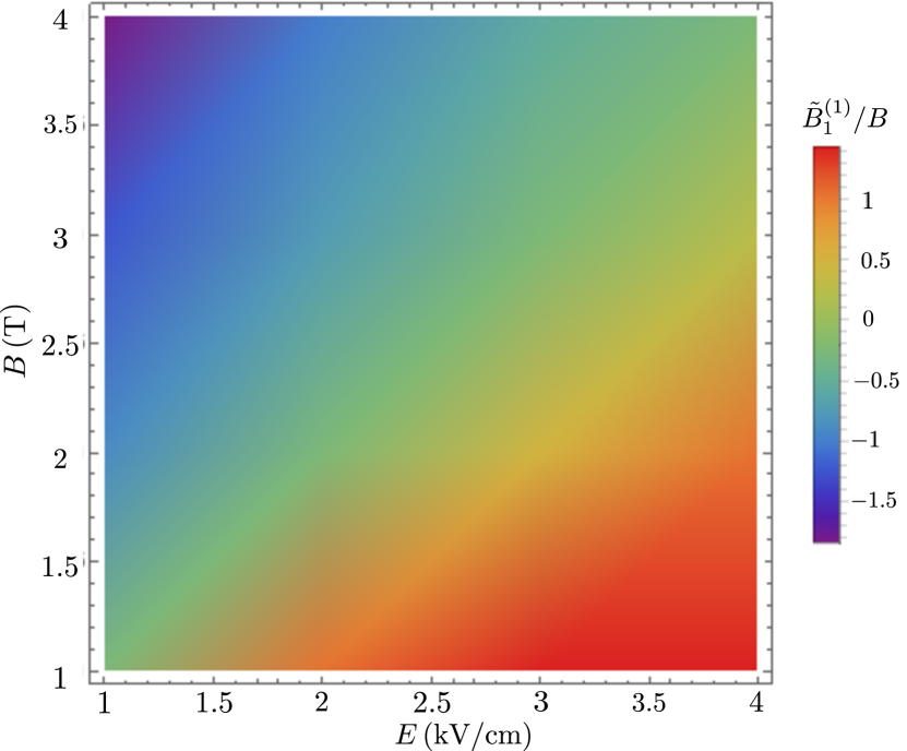
Figure 4: Effective magnetic field component $\tilde{B}^{(1)}_{1}/B$ for external field strengths $1\,\textrm{kV/cm}\leq E\leq 4\,\textrm{kV/cm}$, $1\,\textrm{T}\leq B\leq 4\,\textrm{T}$.

In order to calculate the excitonic spectrum within this approximation, we use the renormalized Luttinger parameters to define effective masses $\mu^{(\alpha)}_{i},\ i=x,y,z$, as

$$\frac{1}{\mu^{(\alpha)}_{i}} \equiv 1+4\frac{\gamma_{2}}{\gamma^{{}^{\prime}}_{1}}\left[1-\frac{3}{2}\gamma^{(\alpha)}_{2,i}(\boldsymbol{r}_{\rm min})\right],$$

$$\gamma^{(\alpha)}_{ij} \equiv -\frac{6\gamma_{3}}{\gamma^{{}^{\prime}}_{1}}\gamma^{(\alpha)}_{3,ij}(\boldsymbol{r}_{\rm min}).$$ (38)

This means that for all three potential curves we obtain effective Hamiltonians $H^{(\alpha)}_{\rm eff}$ with

$$H^{(\alpha)}_{\rm eff} = \sum_{i}\frac{\pi^{(\alpha)2}_{i}}{2\mu^{(\alpha)}_{i}}+\sum_{i\not=j}\gamma^{(\alpha)}_{ij}\pi^{(\alpha)}_{i}\pi^{(\alpha)}_{j}+V_{\alpha}(\boldsymbol{r}),$$

$$\pi^{(\alpha)}_{i} = p_{i}-q\tilde{A}^{(\alpha)}_{i}.$$ (39)

Analogous to the strong electric-field approximation, the exact interaction potentials $V_{\alpha}(\boldsymbol{r})$ can be expanded around their minimum positions $\boldsymbol{r}^{(\alpha)}_{\rm min}$. By defining the frequencies

$$C^{(\alpha)}_{ij}\equiv\frac{\partial^{2}}{\partial x_{i}\partial x_{j}}V_{\alpha}(\boldsymbol{r})|_{\boldsymbol{r}=\boldsymbol{r}_{\rm min}},$$ (40)

the exact potentials can be approximated by

$$V^{(\alpha)}_{\rm h}(\boldsymbol{r}) = V^{(\alpha)}_{\rm min}+\frac{1}{2}\bigg{(}C^{(\alpha)}_{xx}x^{2}+C^{(\alpha)}_{yy}y^{2}+C^{(\alpha)}_{zz}z^{2}$$

$$+ C^{(\alpha)}_{xy}xy+C^{(\alpha)}_{xz}xz+C^{(\alpha)}_{yz}yz\bigg{)}$$

with $V^{(\alpha)}_{\rm min}\equiv V_{\alpha}(\boldsymbol{r}^{(\alpha)}_{\min})$. Together with the $\pi^{(\alpha)}_{i}$-dependent terms in Eq. (III.2), the effective excitonic Hamiltonian is bilinear in the spatial and canonical momentum coordinates $\boldsymbol{r}$ and $\boldsymbol{p}$, respectively, and can thus be written as

$$H^{(\alpha)}_{\rm eff}=\boldsymbol{x}^{T}\mathcal{H}^{(\alpha)}_{\rm eff}\boldsymbol{x},\ \ \boldsymbol{x}=(x\ y\ z\ p_{x}\ p_{y}\ p_{z})^{T}$$ (41)

in which $\mathcal{H}^{(\alpha)}$ is a $(6\times 6)$-dimensional real, symmetric and positive definite matrix (see App. B). We note that, if the terms $\gamma^{(\alpha)}_{ij},C^{(\alpha)}_{ij},\ i\not=j$ are negligible, the effective Hamiltonians $H^{(\alpha)}_{\rm eff}$ are sums of three harmonic oscillators of charge $q$ and masses $\mu^{(\alpha)}_{i}$ in external effective magnetic fields. This problem can be solved by applying an unitary transformation that decouples the different degrees of freedom, and where the spectrum is determined by the coefficients $C^{(\alpha)}_{ii}$ [24; 28].

In order to calculate the eigenenergies of Eq. (41) exactly, we apply Williamson’s theorem [39; 40] which states that there exists a symplectic matrix $S^{(\alpha)}\in\textrm{Sp}(6,\mathbb{R})$ such that

$$\mathcal{H}^{(\alpha)}_{\rm eff}=S^{(\alpha)}D^{(\alpha)}S^{(\alpha)T}$$ (42)

with $D^{(\alpha)}=\textrm{diag}(\lambda^{(\alpha)}_{1},\lambda^{(\alpha)}_{2},\lambda^{(\alpha)}_{3},\lambda^{(\alpha)}_{1},\lambda^{(\alpha)}_{2},\lambda^{(\alpha)}_{3})$, $\lambda^{(\alpha)}_{i=1,2,3}>0$. Importantly, the components of the transformed coordinate vector $\boldsymbol{q}^{(\alpha)}=S^{(\alpha)}\boldsymbol{x}$ fulfill the same commutation relation as the $\boldsymbol{x}_{i}$, i.e.

$$[q^{(\alpha)}_{i},q^{(\alpha)}_{j}]=iJ_{ij},\ \ J=\begin{bmatrix}0&1_{n}\\ -1_{n}&0\end{bmatrix}$$ (43)

where $1_{n}$ denotes the $n\times n$ unit matrix. In the new coordinates, the Hamiltonian $H^{(\alpha)}_{\rm eff}$ is given by

$$H^{(\alpha)}_{\rm eff}=\sum^{3}_{i=1}\lambda^{(\alpha)}_{i}\left[q^{(\alpha)2}_{i}+q^{(\alpha)2}_{i+2}\right],$$ (44)

i.e., we find three uncoupled harmonic oscillators with frequencies $\tilde{\omega}^{(\alpha)}_{i}=2\lambda^{(\alpha)}_{i},\ i=1,2,3$. This means that the eigenenergies of $H^{(\alpha)}_{\rm eff}$ are

$$\varepsilon^{(\alpha)}_{n_{1}n_{2}n_{3}}=\sum^{3}_{i=1}\tilde{\omega}^{(\alpha)}_{i}(n_{i}+\frac{1}{2}),\ \tilde{\omega}^{(\alpha)}_{i}\equiv 2\lambda^{(\alpha)}_{i},\ \ n_{i}\in\mathbb{N}_{0}.$$ (45)

Similar to a three-dimensional harmonic oscillator, the energy spectrum is determined by three separate energy spacings $\tilde{\omega}^{(\alpha)}_{i},\ i=1,2,3$.

Analogous to the strong electric-field limit, we define the quantity $\tilde{\eta}^{(\alpha)}$ that measures the energy difference between the potential depth and the ground-state energy, and obtain

$$\tilde{\eta}^{(\alpha)}=1-\frac{1}{2V^{(\alpha)}_{\rm d}}\sum\limits_{i=1}^{3}\tilde{\omega}^{(\alpha)}_{i}.$$ (46)

In Fig. 5, we show the energy difference $\tilde{\eta}^{(1)}$ for applied field strengths of $1\,\textrm{kV/cm}\leq E\leq 4\,\textrm{kV/cm}$ and $1\,\textrm{T}\leq B\leq 4\,\textrm{T}$. As before, one observes that, for increasing electric field strength, $\tilde{\eta}^{(1)}$ becomes negative, which means that the ground state energy lies above the potential depth, i.e. no bound state is present. However, for low electric fields and high magnetic fields of around $B=4\,\textrm{T}$, we find a regime in which $\tilde{\eta}^{(1)}$ is positive. In Fig. 5, this region is indicated by the shaded box. This result is reasonable as for increasing magnetic field strengths the potential depth increases as well. This means that, for sufficiently strong magnetic fields, the potential wells are deep enough to support bound excitonic giant-dipole states.

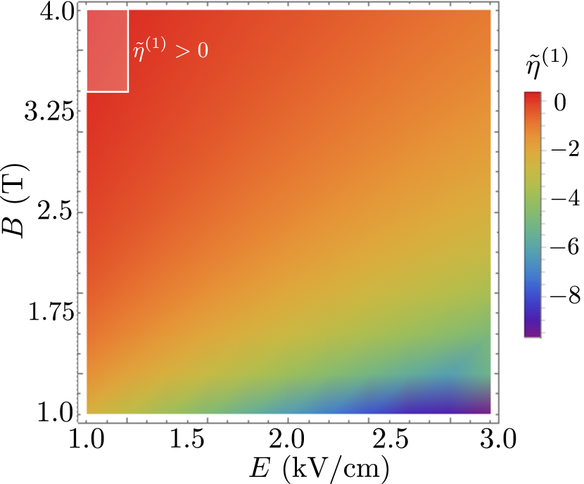
Figure 5: Density plot of $\tilde{\eta}^{(1)}$ for $1\,\rm kV/cm\leq E\leq 3\,\rm kV/cm$ and $1\,\rm{T}\leq B\leq 4\,\rm T$. For large electric fields, $\tilde{\eta}^{(1)}<0$, while for strong magnetic fields one finds $\tilde{\eta}^{(1)}>0$. This region is indicated by the shaded box.

In Tab. 1, we present the frequencies $\tilde{\omega}^{(\alpha)}_{k}$ for the first, third and fifth potential surface for field strengths of $B=4\,\textrm{T}$ and $E=1\,\textrm{kV/cm}$. The frequencies for $\alpha=2,4,6$ are not explicitly shown as they are close to the values for the adjacent potential surface. One observes that, for all potentials one obtains two frequencies with values in the range of $87\,\mu\textrm{eV}-242\,\mu\textrm{eV}$. The third frequency is always larger and lies between $949\,\mu\textrm{eV}$ for the third and $1.58\,\textrm{meV}$ for the first potential curve. Compared to the potential depths of the corresponding surfaces, e.g. $V^{(1)}_{\rm d}=1.05\,\textrm{meV}$, the frequencies with $k=3$ are rather large, meaning that it is only possible to excite one state in the corresponding mode before one exceeds the potential depth and the harmonic approximation breaks down. However, as the frequencies of the remaining modes are smaller, one can easily excite a few states that are still bound deep within the potential surfaces.

	$1$	$2$	$3$
$1$	$87$	$142$	$1580$
$3$	$102$	$161$	$1366$
$5$	$114$	$242$	$949$

Table 1: Excitonic frequencies $\tilde{\omega}^{(\alpha)}_{k}$ in $\mu\textrm{eV}$ for $B=4\,\textrm{T},\ E=1\,\textrm{kV/cm}$.

If we compare the frequencies $\tilde{\omega}^{(\alpha)}_{k}$ with the energetic spacing $\Delta_{\alpha}$, we find that $\textrm{min}(\tilde{\omega}^{(\alpha)}_{k=1,2,3})\gg\Delta_{\alpha}\ \forall\alpha$, i.e. the frequencies are much larger than the spacing between adjacent potential surfaces. For this reason, we exspect a strong mixing between the potential surfaces in the case we include intrasurface couplings.

Finally, we can determine the eigenstates by using the fact that the transformed effective Hamiltonian, Eq.  (44), is a sum of three decoupled harmonic oscillators. Thus, we can construct ladder operators $a^{(\alpha)(\dagger)}_{k},\ k=1,2,3$ as

$$a^{(\alpha)(\dagger)}_{k}=\frac{1}{2}\left(q^{(\alpha)}_{k}\pm iq^{(\alpha)}_{k+2}\right).$$ (47)

From here, the giant-dipole eigenstates $|n_{1}n_{2}n_{3}\rangle$ are constructed via

$$|n_{1}n_{2}n_{3}\rangle_{\alpha}=\frac{1}{\sqrt{n_{1}!n_{2}!n_{3}!}}$$

$$\times\left(a^{(\alpha)\dagger}_{1}\right)^{n_{1}}\left(a^{(\alpha)\dagger}_{2}\right)^{n_{2}}\left(a^{(\alpha)\dagger}_{3}\right)^{n_{3}}|0\rangle.$$ (48)

Using the transformation matrix $S^{(\alpha)}$ from Eq. (42), both the spatial and momentum coordinates can be expressed in terms of the ladder operators and vice versa.

IV Full excitonic spectra

In order to provide a full analysis of the excitonic spectra, we next consider a full diagonalization approach to calculate the corresponding excitonic eigenenergies and states. Here, we are mostly interested in the determination of the ground state and the lowest lying giant-dipole states. In order to compute them most efficiently, one has to choose a basis set adapted to the properties of the system. As we are interested in the properties of the potentially bound excitonic giant-dipole states that are localized in the outer potential wells, it is clear that one should choose a set of basis functions that are also localized around the outer potential minima of the giant-dipole potential surfaces. As we have seen in Sec. III in case of the adiabatic approximation, one obtains a set of effective giant-dipole Hamiltonians that can be diagonalized separately from one another. In this case, one obtains a set of basis functions that inherently possess the desired properties required for them to be a good choice for the diagonalization procedure. However, as we are interested in the lowest lying giant-dipole states, we use the fact that for the considered field strength regime the lowest potential energy surface is mostly determined by the first term in the expression of the excitonic giant-dipole potential [see Eq. (7)]. Expanding this term up to second order around the minimum position $z_{\rm{min}}$, i.e.

$$\Omega_{1}B^{2}(y^{2}+z^{2})+Ez-\frac{1}{r}$$

$$\approx V_{\rm{min}}+\frac{1}{2}\omega^{2}_{x}x^{2}+\frac{1}{2}\omega^{2}_{y}y^{2}+\frac{1}{2}\omega^{2}_{z}(z-z_{\rm{min}})^{2},$$ (49)

we define the basis functions $|\psi_{n_{x},n_{1},n_{2}}\rangle$ for our diagonalization procedure to be the giant-dipole eigenfunctions of a single particle of mass $\mu=1$, charge $q$, trapping frequencies $\omega_{i=x,y,z}$ and external fields $\boldsymbol{B}$ and $\boldsymbol{E}$, respectively. Together with the basis states of the spin-1 and spin-1/2 Hilbert space $|1,m\rangle\otimes|1/2,m_{s}\rangle,$ we define the following basis states

$$|\gamma,m,m_{s}\rangle\equiv|\psi_{n_{x},n_{1},n_{2}}\rangle\otimes|1,m\rangle\otimes|\frac{1}{2},m_{s}\rangle$$ (50)

$$n_{i}=0,1,2,...\ \ \ m=0,\pm 1\ \ \ m_{s}=\pm\frac{1}{2}.$$ (51)

For the exact diagonalization scheme we have calculated the matrix elements of the excitonic Hamiltonian (12), where the giant-dipole potential is approximated by Eq. (49). Together with the six-dimensional spin-space, one obtains a $6(N_{x,\rm{max}}+1)(N_{1,\rm{max}}+1)(N_{2,\rm{max}}+1)$-dimensional matrix representation for the excitonic giant-dipole Hamiltonian, where $N_{i,\rm{max}}$ denote the maximal number of basis functions used within the chosen basis set. Throughout our analysis, we obtained sufficient numerical convergence using $N_{x,\rm{max}}=N_{1,\rm{max}}=15,\ N_{2,\rm{max}}=5$, which yields a basis set of $9216$ states.

IV.1 Magnetic field in [100]-direction

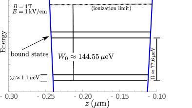
Figure 6: Bound excitonic states in the energetically lowest potential surface ($x,y=0$). The ground state possesses a binding energy of $144.55\,\mu\textrm{eV}$, we find four bound states in total. The external field parameter are $B=4\,\textrm{T}$, $E=1\,\textrm{kV/cm}$.

In Fig. 6, we show the lowest bound excitonic giant-dipole states for $B=4\,\textrm{T}$ and $E=1\,\textrm{kV/cm}$, respectively. For these field strengths, the ground state possesses an approximate binding energy of $W_{0}\approx 144.55\,\mu\textrm{eV}$. In our analysis, we estimate the binding energy of a certain state to be the energetic separation of the eigenenergy to the ionization limit of the lowest potential surface. The binding energies of the excited states are of similar order of magnitude, namely in the range between $144\,\mu\textrm{eV}$ and $68\,\mu\textrm{eV}$. In total, we find four bound states.

For all applied field strengths, the series of binding energies of the giant-dipole states can be cast into the form

$$W_{n,m}=W_{0}-n\Omega-m\omega,\ n\in\mathbb{N}_{0},\ m\in\{0,1\},$$ (52)

where $\Omega,\omega>0$, $\Omega\gg\omega$, and $W_{0}$ denotes the ground-state binding energy.

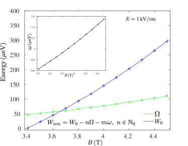
Figure 7: Binding energy $W$ (blue dots) and energy scale $\Omega$ (green dots) as a function of the magnetic field $B$. The inset shows the smaller energy scale $\omega$ as a function of $B$.

In Fig. 7, we show the magnetic-field dependence of the binding energy (blue dots) and the larger energy scale $\Omega$ (green dots) for $3.4\,\textrm{T}\leq B\leq 4.5\,\textrm{T}$ for fixed electric field strength $E=1\,\textrm{kV/cm}$. One observes that the ground-state binding energy increases nearly linearly with increasing magnetic field strength from $W_{0}=1.92\,\mu\textrm{eV}$ ($B=3.4\,\textrm{T}$) to $W_{0}=297.05\,\mu\textrm{eV}$ ($B=4.5\,\textrm{T}$). The same holds for $\Omega$, which increases from $\Omega=47.67\,\mu\textrm{eV}$ ($B=3.4\,\textrm{T}$) to $\Omega=110.491\,\mu\textrm{eV}$ ($B=4.5\,\textrm{T}$). The inset in Fig. 7 shows the magnetic-field dependence of the smaller energy scale $\omega$, with an almost linear increase from $\omega=0.63\,\mu\textrm{eV}$ to $\omega=1.55\,\mu\textrm{eV}$. This can be explained by the fact that, with increasing magnetic-field strength, the spatial confinement within the potential surface increases as well, which leads to larger energetic separation of adjacent energy levels.

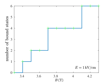
Figure 8: The number of bound excitonic giant-dipole states as a function of the magnetic field strength $B$. For $B<3.4\,\textrm{T}$ no bound states are present, from there the number of bound states increase up to six for $B\geq 4.1\,\textrm{T}$.

The number of bound states depends on whether the large energy scales $W_{0},\Omega$ and $\omega$ are related to the potential depth of the energetically lowest potential surface. In Fig. 8, we show the number of bound states as a function of the magnetic field strength for $E=1\,\textrm{kV/cm}$. Below $B\lesssim 3.4\,\textrm{T}$, the potential well is too shallow and no bound excitonic giant-dipole states can be formed. At $B=3.4\,\textrm{T}$, the potential becomes slightly deeper than $W_{0}$, which means that one bound state fits into the well. Increasing $B$ leaves the number of bound states unchanged as long as the potential well is smaller than $W_{0}+\omega$ which is true for $3.4\,\textrm{T}\leq B\leq 3.5\,\textrm{T}$. Beyond that, we find two bound states. This sequence continues until the maximal number of six bound states is reached for $B\gtrsim 4.3\,\textrm{T}$. Note that one cannot arbitrarily increase the magnetic field strength to further increase the number of bound states, as the outer potential wells cease to exist when the magnetic field contributions are stronger than the Stark term provided by the electric field in Eq. (7).

One effect of the relatively strong magnetic field is that the bound states imply an electron-hole separation well below one micrometer, namely of around $200\,\textrm{nm}$ for $B=4\,\textrm{T}$. In this case, the excitonic dipole moment can be estimated to be around $120\,\textrm{Debye}$, which is less than expected from the analysis performed in Ref. [25] but still large compared to normal atomic and excitonic dipole strengths.

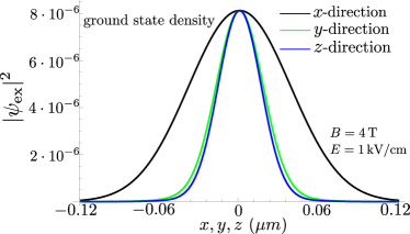
Figure 9: Cuts through the ground-state probability density along the $x$, $y$, and $z$-direction, respectively. Due to the different spatial confinement ($\omega_{y}/\omega_{x}\approx 4.4,\ \omega_{z}/\omega_{x}\approx 4.1$), the spatial extension differs along the different directions.

Apart from the excitonic eigenenergies, the exact diagonalization scheme also provides the excitonic eigenfunctions. For instance, in Fig. 9 we show the (Gaussian) ground-state probability density along the $x$, $y$ and $z$-directions, respectively. While the spatial extension is nearly equal in the $y$ and $z$-directions, the extension in the $x$-direction is much larger. In particular, for $B=4\,\textrm{T}$ and $E=1\,\textrm{kV/cm}$ we find that $\omega_{y}/\omega_{x}\approx 4.4$ and $\omega_{z}/\omega_{x}\approx 4.1$, a slightly smaller spatial confinement in the $y$-direction than in the $z$-direction, which is reflected in the ground-state probability density in Fig. 9.

IV.2 Fields in arbitrary directions

So far, we have analyzed the case of the magnetic and electric field being parallel to the $[100]$ and $[001]$ directions, respectively. In order to provide some insight into different field configurations, we now consider the case that the both magnetic and electric fields are oriented along arbitrary directions, whilst still being perpendicular with respect to one another. Introducing the spherical angles $\phi_{B}$ and $\theta_{B}$ of the magnetic field vector $\boldsymbol{B}$, the unit vectors $\boldsymbol{b}$ and $\boldsymbol{e}$ for the magnetic and electric fields can be expressed as

$$\boldsymbol{b}=\begin{pmatrix}\cos(\phi_{B})\sin(\theta_{B})\\ \sin(\phi_{B})\sin(\theta_{B})\\ \cos(\theta_{B})\end{pmatrix},$$ (53)

$$\boldsymbol{e}=\begin{pmatrix}-\cos(\phi_{B})\cos(\theta_{B})\\ -\sin(\phi_{B})\cos(\theta_{B})\\ \sin(\theta_{B})\end{pmatrix}.$$ (54)

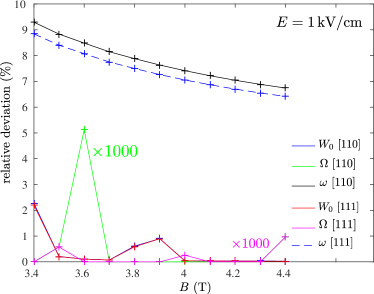
Figure 10: Relative deviation of the energies scales $\Omega,\omega$ and $W_{0}$ for magnetic field orientations $B||[110]$ and $B||[111]$, respectively. The largest deviation of around $9\%$ is found for $\omega\ [110]$ and $\omega\ [111]$ in the case of $B=0$. For $W_{0}$ is deviation is smaller, namely $2\%$ and less. In the case of $\Omega$ is smallest relative deviations are found with $0.005\%$ and much less.

For arbitrary field directions, the potential minimum is still to be found in the direction of the electric field. In order to introduce local giant-dipole states for the exact diagonalization procedure, one would have to introduce a set of local coordinates. However, this inconvenience can be overcome by rotating the coordinate system in such a way that the magnetic field direction coincides with the quantization axis of the system. In particular, we rotate the coordinate system by

$$R=\begin{bmatrix}\cos(\phi_{B})\sin(\theta_{B})&\sin(\phi_{B})\sin(\theta_{B})&\cos(\theta_{B})\\ -\sin(\phi_{B})&\cos(\phi_{B})&0\\ -\cos(\phi_{B})\cos(\theta_{B})&-\sin(\phi_{B})\cos(\theta_{B})&\sin(\theta_{B})\\ \end{bmatrix},$$

The rotation of the system is performed by rotating the excitonic Hamiltonian, in particular, the irreducible tensor representation given by Eq. (2) transforms by applying Wigner $D$-matrices. In App. E, we give details of the transformed excitonic Hamiltonians for magnetic fields along the $[110]$ and $[111]$ directions, respectively.

The calculation of the excitonic giant-dipole eigenenergies for the different field configurations has been performed analogously to the magnetic field along $[100]$. In particular, the giant-dipole potential surfaces were expanded around the potential minimum up to second order, then appropriate basis sets were defined in order to perform an exact diagonalization for the numerical determination of the eigenenergies. We find that for all considered field configurations the excitonic spectra are determined by two distinct energy scales as observed in Sec. IV. In particular, we find that for all field orientations the energy scales $\Omega,\omega$ as well as the ground-state binding energy $W_{0}$ differ only slightly from another.

In Fig. 10, we show the relative deviation of the energies $\Omega,\omega$ and $W_{0}$ for $B||[110]$ and $B||[111]$ from their values obtained in the case of $B||[100]$ (see Fig. 7). The largest deviation is found for $\omega$ with a relative deviations between $7\%$ and $9\%$. For increasing magnetic field strength the deviations are monotonically decreasing. The relative deviations of $W_{0}$ the relative are even smaller, they are found to be around $2\%$ for $B=0$ and nearly vanish for $B\geq 4\,\textrm{T}$. Furthermore, we see that there are hardly any deviations for the energies scales $W_{0}\,([110])$ and $W_{0}\,([111])$. Finally, the smallest relative deviations are found for $\Omega\,([110])$ and $\Omega\,([111])$, with the largest deviation of merely $0.005\%$ for $\Omega\,([110])$, and around $0.001\%$ for $\Omega\,([111])$.

V Summary and Conclusions

In the present article, we have calculated the eigenspectra of giant-dipole excitons in $\textrm{Cu}_{2}\textrm{O}$ subject to crossed electric and magnetic fields. In particular, we have derived the irreducible tensor representation of excitons in crossed electric and magnetic fields in cuprous oxide. In this way, the analysis of the excitonic systems for arbitrary field strength and arbitrary field configurations is straightforward as the irreducible representations can be used to transform the system in such a way that the magnetic field coincides with the quantization axis.

In particular, we have calculated the eigenenergies of giant-dipole excitons in $\textrm{Cu}_{2}\textrm{O}$ for arbitrary field strengths and orientations by applying both an adiabatic approximation as well as an exact diagonalization approach. We verify that, in order to find bound excitonic giant-dipole states, one requires sufficiently deep potential surfaces. As the depths of the considered potential surfaces strongly depend on the applied field strengths, bound states are only possible in the limit of weak electric and strong magnetic fields. For instance, we find bound states for field strengths of around $E\approx 1\,\textrm{kV/cm}$ and $3.4\,\textrm{T}\leq B\leq 4.3\,\textrm{T}$. For all field orientations, the corresponding level spacings are determined by two energy scales which are of the order of $1-2\,\mu\textrm{eV}$ and $100\,\mu\textrm{eV}$, respectively. The number of bound states is comparable small, for the considered field strengths we find between one and six bound states for all field orientations.

An open question is the experimental preparation and verification of the the existence of these excitonic giant-dipole states. The latter could, in principle, be achieved via spectroscopic measurements of the excitonic resonances which should be visible in microwave spectroscopy. An alternative approach might be the direct measurement of the large electric dipole moment which can be estimated to be of the order of several tens of thousand Debye.

Another yet unsolved question is how to prepare those exotic excitonic states. Due to the large spatial separation between the outer potential wells and the Coulomb-dominated region, a direct radiative transfer via external lasers is unlikely as the overlap between the giant-dipole wave functions and low-lying exciton states in the inner region is very small.

However, one possible approach may be to use the field-free excitation of highly excited Rydberg excitons. Applying time-dependent external fields hereafter, one might be able to adiabatically transfer the Rydberg state into the desired field-dressed giant-dipole configuration. For the determination of a possible propagation scheme one has to consider that, although classical trajectory simulations has already provided some understanding for a possible preparation scheme for atomic giant-dipole states [41], the setup for excitonic states is more complicated due to the complex spin-structure. In particular, one has to consider six distinct coupled potential surfaces, causing non-adiabatic state transfer among those. In order to include non-adiabatic transitions between the potential surfaces, one may adapt a method from molecular dynamics calculations known as surface hopping [42; 43] which partially incorporates the non-adiabatic effects by including excited adiabatic surfaces in the calculations, and allowing for transitions between these surfaces. An alternative approach might be to perform a full quantum mechanical analysis to achieve an optimal state transfer starting from an appropriate initial excitonic state. This belongs to a general class of problems known as control theory [44; 45], where one is interested in finding a protocol to change addressable system parameters such that a certain optimal criterion is achieved.

Yet another possibility to create excitonic giant-dipole states might be to directly start in the field-dressed configuration and to excite ground-state excitons directly into the continuum, that may recombine into states localized in the outer potential wells due to radiative decay, interspecies scattering events or phonon-induced de-excitation. Especially the last decay channel might be of particular interest as it is induced by the solid-state environment and which is not present in ultra-cold atomic gases. In summary, the preparation of excitonic giant-dipole states provides a plethora of interesting research directions that can be addressed in future theoretical as well as experimental studies.

Appendix A Excitonic parameters

In Tab. 2 we list the excitonic parameters used throughout this work.

Luttinger parameters	$\gamma_{1},\gamma_{2},\gamma_{3}$	$1.818,0.803,-0.397$
	$\gamma^{{}^{\prime}}_{1},\kappa$	$2.83,-0.5$
Hartree energy	$\mathcal{H}_{\rm ex}$	$170\,\rm meV$
(excitonic) Bohr radius	$a_{\rm ex}$	$1.15\,\rm nm$
magnetic flux density	$B_{\rm ex}$	$520.6\,\rm T$
electric field strength	$E_{\rm ex}$	$1.518\,\rm MV/cm$
momentum	$P_{\rm ex}$	$4.8\times 10^{-2}\hbar/a_{0}$
gap energy	$E_{g}$	$2.17208\,\rm eV$
spin-orbit coupling	$\Delta$	$133.8\,\rm meV$
Bohr magneton	$\mu_{B}$	$57.88\,\mu\rm eV/T$

Table 2: Excitonic Hartree energy $\mathcal{H}_{\rm ex}$, Bohr radius $a_{\rm ex}$, external field strengths $(B_{\rm ex},E_{\rm ex})$ and momentum $P_{\rm ex}$. In addition, the spin-orbit and magnetic coupling $(\Delta,\mu_{B})$ is presented as well as the Luttinger parameters used throughout this work.

Appendix B Williamson’s theorem

Let $M$ be a positive-definite symmetric real $2n\times 2n$ matrix. In this case the following theorem holds [39]:

• There exists $S\in\textrm{Sp}(2n,\mathbb{R})$ such that

  $$M = S^{T}DS,\ \ \ D=\textrm{diag}(\Lambda,\Lambda),$$

  $$\Lambda = \textrm{diag}(\lambda_{1},...,\lambda_{n}),\ \ \ \textrm{with}\ \ \ \lambda_{i}\in\mathbb{R}^{>0}.$$

• The entries $\lambda_{i}$ of $\Lambda$ are defined by the condition that $\pm i\lambda_{i}$ is an eigenvalue of $J_{n}M$ where

  $$J_{n}=\begin{bmatrix}0&1_{n}\\ -1_{n}&0\\ \end{bmatrix}.$$

• The sequence $\lambda_{1},...,\lambda_{n}$ does not depend, up to a reordering of its terms, on the choice of $S$ diagonalizing $M$.

We introduce ${\bf q}=S{\bf x}$ with $S\in\textrm{Sp}(6,\mathbb{R})$. In this case, the canonical commutator relations are preserved, i.e. $[q_{i},q_{j}]=iJ_{3,ij}$.

Appendix C Irreducible representation of kinetic and potential energy

The irreducible tensor representation of the kinetic energy term $T$ and the potential energy $V$ for a magnetic field orientation of $\boldsymbol{B}||[100]$ discussed in Sec. II is given by

$$T=\frac{\boldsymbol{\pi}^{2}}{2}-\frac{\mu^{\prime}}{3}\{(\Pi^{(2)}\cdot I^{(2)})\}$$

$$+\frac{\delta^{\prime}}{3}\bigg{(}\sum_{k=\pm 4}\{[\Pi^{(2)}\times I^{(2)}]^{(4)}_{k}\}+\frac{\sqrt{70}}{5}\{[\Pi^{(2)}\times I^{2}]^{(4)}_{0}\}\bigg{)},$$

$$V = \left(\Omega_{1}\tilde{K}^{2}+E^{(1)}\cdot r^{(1)}-\frac{1}{r}\right)-\frac{\lambda^{\prime}}{3}(\tilde{K}^{(2)}\cdot I^{(2)})$$

$$+\frac{\xi^{\prime}}{3}\left(\sum_{k=\pm 4}[\tilde{K}^{(2)}\times I^{(2)}]^{(4)}_{k}+\frac{\sqrt{70}}{5}[\tilde{K}^{(2)}\times I^{2}]^{(4)}_{0}\right)$$

$$+H_{\rm so}+H_{\rm B}$$

with $\lambda^{\prime}=\frac{2}{5}(\Omega_{3}+\Omega_{2}),\ \xi^{\prime}=\Omega_{3}/3-\Omega_{2}/2$ and

$$H_{\rm so} = \frac{2}{3}\bar{\Delta}\left(1+S^{(1)}_{h}\cdot I^{(1)}\right),$$

$$H_{\rm B} = \bar{\mu}_{B}[(3\kappa+\frac{g_{s}}{2})I^{(1)}\cdot B^{(1)}-g_{s}S^{(1)}_{h}\cdot B^{(1)}].$$

Appendix D The excitonic Hamiltonian in adiabatic approximation

In Eq. (41), we introduced the matrix representation of the excitonic Hamiltonian,

$$H^{(\alpha)}_{\rm eff}=\boldsymbol{x}^{T}\mathcal{H}^{(\alpha)}_{\rm eff}\boldsymbol{x},\ \ \ \textrm{with}\ \ \ \mathcal{H}^{(\alpha)}_{\rm eff} = A^{T}MA,$$

$$\boldsymbol{x} = (x\ y\ z\ p_{x}\ p_{y}\ p_{z})^{T}.$$

The matrices

$$M=\textrm{diag}(P,Q)\ \ \ \textrm{and}\ \ \ A=\begin{bmatrix}I_{3}&0\\ W&I_{3}\\ \end{bmatrix}$$

are given in block form, the submatrices $P,Q,W$ and $I_{3}$ are given by

$$P = \frac{1}{2}\begin{bmatrix}C^{(\alpha)}_{xx}&C^{(\alpha)}_{xy}&C^{(\alpha)}_{xz}\\ C^{(\alpha)}_{xy}&C^{(\alpha)}_{yy}&C^{(\alpha)}_{yz}\\ C^{(\alpha)}_{xz}&C^{(\alpha)}_{yz}&C^{(\alpha)}_{zz}\\ \end{bmatrix},\ Q=\begin{bmatrix}\frac{1}{2\mu^{(\alpha)}_{x}}&\gamma^{(\alpha)}_{xy}&\gamma^{(\alpha)}_{xz}\\ \gamma^{(\alpha)}_{xy}&\frac{1}{2\mu^{(\alpha)}_{y}}&\gamma^{(\alpha)}_{yz}\\ \gamma^{(\alpha)}_{xz}&\gamma^{(\alpha)}_{yz}&\frac{1}{2\mu^{(\alpha)}_{z}}\\ \end{bmatrix}$$

$$W = \frac{1}{2}\begin{bmatrix}0&0&0\\ 0&0&q\tilde{B}^{(\alpha)}_{z}\\ 0&-q\tilde{B}^{(\alpha)}_{z}&0\\ \end{bmatrix},\ I_{3}=\begin{bmatrix}1&0&0\\ 0&1&0\\ 0&0&1\\ \end{bmatrix}.$$

Appendix E Field-dressed excitonic Hamiltonians

The irreducible tensor representations of field-dressed excitonic Hamiltonians for $\boldsymbol{B}||[110]$ and $\boldsymbol{B}||[111]$, respectively, are listed below.

Magnetic field in [110] direction

$$H_{\rm ex}=\frac{\boldsymbol{\pi}^{2}}{2}-\frac{\mu^{\prime}}{3}\{(\Xi^{(2)}\cdot I^{(2)})+\frac{\delta^{\prime}}{4}\big{(}\sum_{k=\pm 4}\{[\Xi^{(2)}\times I^{(2)}]^{(4)}_{k}\}\big{)}$$

$$-\frac{\sqrt{7}}{6}\delta^{\prime}\big{(}\sum_{k=\pm 2}\{[\Xi^{(2)}\times I^{(2)}]^{(4)}_{k}\}+\sqrt{\frac{1}{10}}\{[\Xi^{(2)}\times I^{(2)}]^{(4)}_{0}\}\big{)}$$

$$+\bigg{(}\Omega_{1}\tilde{K}^{2}+E^{(1)}\cdot r^{(1)}-\frac{1}{r}\bigg{)}+H_{\rm so}+H_{\rm B}.$$

Magnetic field in [111] direction

$$H_{\rm ex}=\frac{\boldsymbol{\pi}^{2}}{2}-\frac{\mu^{\prime}}{3}\{\Xi^{(2)}\cdot I^{(2)})\}$$

$$+\frac{4}{27}\delta^{\prime}\big{(}\sum_{k=\pm 3}k\{[\Xi^{(2)}\times I^{(2)}]^{(4)}_{k}\}-\sqrt{\frac{63}{10}}\{[\Xi^{(2)}\times I^{(2)}]^{(4)}_{0}\}\big{)}$$

$$+\left(\Omega_{1}\tilde{K}^{2}+E^{(1)}\cdot r^{(1)}-\frac{1}{r}\right)+H_{\rm so}+H_{\rm B}.$$

References

- [1] J. Frenkel, Phys. Rev. 37, 1276 (1931).
- [2] N. F. Mott, Trans. Fraraday Soc. 34, 500 (1938).
- [3] E. F. Gross and N. A. Karryjew, Dokl. Akad. Nauk SSSR 84, 471 (1952).
- [4] M. Hayashi and K. Katsuki, J. Phys. Soc. Jpn. 7, 599 (1952).
- [5] E. F. Gross, Nuovo Cimento 3, 672 (1956).
- [6] T. Kazimierczuk et al., Nature (London) 514, 343 (2014).
- [7] A. Baldereschi and N. C. Lipari, Phys. Rev. B 3, 439 (1970).
- [8] A. Baldereschi and N. C. Lipari, Phys. Rev. B 8, 2697 (1973).
- [9] A. Baldereschi and N. C. Lipari, Phys. Rev. B 9, 1525 (1973).
- [10] C. Uihlein, D. Fröhlich, and R. Kenklies, Phys. Rev. B 23, 2731 (1981).
- [11] K. Suzuki and J. C. Hensel, Phys. Rev. B 9, 2731 (1974).
- [12] F. Schöne et al., Phys. Rev. B 93, 075203 (2016).
- [13] J. Thewes et al., Phys. Rev. Lett. 115, 027402 (2015).
- [14] V. T. Agekyan, phys. stat. sol. (a) 43, 11 (1977).
- [15] M. Altarelli and N. Lipari, Phys. Rev. B 7, 3798 (1972).
- [16] K. Cho, S. Suga, W. Dreybrodt, and F. Willmann, Phys. Rev. B 11, 1512 (1974).
- [17] M. Semina et al., 24th Int. Symp. “Nanostructures: Physics and Technology”, Saint Petersburg, Russia (2016).
- [18] J. Heckötter et al., Phys. Rev. B 95, 035210 (2017).
- [19] F. Schweiner et al., Phys. Rev. B 95, 035202 (2017).
- [20] F. Schweiner, J. Main, M. Feldmaier, and G. Wunner, Phys. Rev. B 93, 195203 (2016).
- [21] F. Schweiner, J. Main, and G. Wunner, Phys. Rev. Lett. 118, 046401 (2017).
- [22] F. Schweiner, J. Main, and G. Wunner, Phys. Rev. E 95, 062205 (2017).
- [23] F. Schweiner, P. Rommel, J. Main, and G. Wunner, Phys. Rev. B 96, 035207 (2017).
- [24] P. Schmelcher and L. S. Cederbaum, Chem. Phys. Lett. 208, 548 (1993).
- [25] M. Kurz, P. Grünwald, and S. Scheel, Phys. Rev. B 95, 245205 (2017).
- [26] D. Baye, N. Clerbaux, and M. Vincke, Phys. Lett. A 166, 135 (1992).
- [27] I. Dzyaloshinskii, Phys. Lett. A 165, 69 (1992).
- [28] O. Dippel, P. Schmelcher, and L. S. Cederbaum, Phys. Rev. A 49, 4415 (1994).
- [29] J. Shertzer, J. Ackermann, and P. Schmelcher, Phys. Rev. A 58, 1129 (1998).
- [30] P. Schmelcher, Phys. Rev. A 64, 063412 (2001).
- [31] M. Fauth, H. Walther, and E. Werner, Z. Phys. D 7, 293 (1987).
- [32] G. Raithel, M. Fauth, and H. Walther, Phys. Rev. A 47, 419 (1993).
- [33] J. E. Avron, I. W. Herbst, and B. Simon, Ann. Phys. (NY) 114, 431 (1978).
- [34] H. Herold, H. Ruder, and G. Wunner, J. Phys. B 14, 751 (1981).
- [35] B. R. Johnson, J. O. Hirschfelder, and K. H. Yang, Rev. Mod. Phys. 55, 109 (1983).
- [36] J. M. Luttinger, Phys. Rev. 102, 1030 (1956).
- [37] J. M. Luttinger and W. Kohn, Phys. Rev. 97, 869 (1954).
- [38] W. Domcke, D. Yarkony, H. Köppel, Conical Intersections – Electronic Structure, Dynamics and Spectroscopy, Advanced Series in Physical Chemistry, Vol. 15, World Scientific, Singapore (2004)
- [39] J. Williamson, Am. J. Math. 58, 141–163 (1936).
- [40] Kh. D. Ikramov, Moscow University Computational Mathematics and Cybernetics 42, 1 (2018).
- [41] V. Averbukh, N. Moiseyev, P. Schmelcher, and L. S. Cederbaum, Phys. Rev. A 59, 3695 (1999).
- [42] M. F. Herman, J. Chem. Phys. 81(2), 754 (1984).
- [43] J. C. Tully, J. Chem. Phys. 93(2), 1061 (1990).
- [44] J. Werschnik, and E. K. U. Gross, J. Phys B: Atomic, Molecular and Optical Physics 40(18), R175 (2007).
- [45] E. Räsänen, A. Castro, J. Werschnik, A. Rubio, and E. K. U. Gross, Phys. Rev. Lett. 98, 157404 (2007).