Space-time least-squares isogeometric method and efficient solver for parabolic problems

Abstract

In this paper, we propose a space-time least-squares isogeometric method to solve parabolic evolution problems, well suited for high-degree smooth splines in the space-time domain. We focus on the linear solver and its computational efficiency: thanks to the proposed formulation and to the tensor-product construction of space-time splines, we can design a preconditioner whose application requires the solution of a Sylvester-like equation, which is performed efficiently by the fast diagonalization method. The preconditioner is robust w.r.t. spline degree and mesh size. The computational time required for its application, for a serial execution, is almost proportional to the number of degrees-of-freedom and independent of the polynomial degree. The proposed approach is also well-suited for parallelization.

Keywords: Isogeometric analysis, parabolic problem, space-time method, $k$-method, splines, least-squares, Sylvester equation.

1 Introduction

Isogeometric analysis (IGA) is a recent technique for the numerical solution of partial differential equations (PDE), introduced in the seminal paper [24]. IGA is an evolution of classical finite element methods (FEM): the main idea is to use the same functions (splines or generalizations) that represent the computational domain in Computer-Aided Design systems, also in the approximation of the solution. We refer to [12] and [3] for a comprehensive presentation and a mathematical survey of IGA, respectively.

IGA allows to use high-order and high-smoothness functions. The $k$-method, based on splines of degree $p$ and $C^{p-1}$ regularity, delivers higher accuracy per degree-of-freedom, comparing to $C^{0}$ or discontinuous $hp$-FEM [8, 13, 17]. However, the $k$-method also requires ad-hoc algorithms, otherwise when the polynomial degree $p$ increases, the computational cost per degree-of-freedom increases dramatically, both in the formation of the matrix and in the solution of the linear system [11, 36].

In this paper, we design and analyze an isogeometric method for parabolic equations, focusing on the heat equation as model problem. The most common numerical methods for time-dependent PDE are obtained by discretizing separately in time (e.g, by difference schemes) and in space (e.g., by a Galerkin method). We consider instead the alternative approach of discretizing the PDE simultaneously in space and time, that is, the so-called space-time (variational) approach. A first idea of space-time finite element method has been introduced in [19, 33, 34] and developed for the heat conduction problem in [25]. Further pioneering studies on space-time methods have been [39, 43], where the authors consider a Galerkin formulation and add a least-squares operator to enhance stability and mitigate spurious oscillations.

More recently, the mathematical analysis of Galerkin space-time methods for parabolic equations has been developed in [38] for a wavelet discretization, and in [41] for a Galerkin finite element discretization.

In the IGA framework, the idea of using smooth splines in time has been first proposed in [44]. The recent paper [45] applies this concept to a complex engineering simulation. A stabilized space-time isogeometric method for the heat equation has been proposed in [29, 30] and its time-parallel multigrid solver has been developed in [23].

In contrast to the existing space-time IGA works, in this paper we adopt an $L^{2}$ least-squares approximation. The first appearance of a least-squares space-time formulation was in [22]. However, as discussed in [5, 6], the discretized formulation of [22] departs from the least-squares minimization principle. In [5, 6] the authors consider a least-squares finite element method for unsteady fluid dynamics problems. For second-order differential equations, the $L^{2}$ minimization of the equation residual would require $C^{1}$-continuous functions in the spatial variables, however [5, 6] recast the second-order equation into a set of first-order equations, whose least-squares formulation allows $C^{0}$ functions. Furthermore, [5, 6] introduce a time-marching approach to lower the memory requirement and the computational time. Henceforth, the most relevant contributions on space-time least-squares methods have retained these two features: 1) the minimization of first-order residuals and 2) the time-marching technique (similar to the use of time-slabs or discontinuous-in-time approximation). We refer to the book [7] for a review of the literature.

Our work departs from the setting described above: we consider high degree and smoothness splines in time and space with the following implications: 1) exploiting the $C^{1}$-continuity of our approximating function, we directly minimize the second-order residual and 2) we need to solve a global-in-time linear system. Point 1) represents an advantage while point 2) is addressed by exploiting the tensor product structure of the spline basis functions: we do not need to form the global space-time matrix, which is given as sum of Kronecker products of matrices, and we set up a preconditioner that relies on the solution of a Sylvester-like equation. Indeed, the least-squares formulation allows us to use the same preconditioning technique introduced in [35] for the Poisson problem, based the so-called fast diagonalization (FD) method (originally proposed in [31] and more recently discussed in [15]). For the space-time least-squares formulation, the computational cost of the preconditioner setup is at most $O(N_{dof})$ floating-point operations (FLOPs) while its application is $O(N_{dof}^{1+1/d})$ FLOPs, where $d$ is the number of space dimensions and $N_{dof}$ denotes the total number of degrees-of-freedom (for simplicity, here we consider the same number of degrees-of-freedom in time and in each space direction). In our numerical benchmarks the measured computational time of the preconditioner, for serial single-core execution, is close to optimality, that is proportional to $N_{dof}$, with no dependence on $p$. Therefore, the preconditioner is robust with respect to the polynomial degree. Moreover, under the assumption that the coefficients of the equation do not depend on time, our approach requires a significantly small amount of memory compared to other space-time approaches: denoting by $N_{s}$ the total number of degrees-of-freedom in space (and assuming the number of degrees-of-freedom in time is not too large, as in typical applications) the storage cost is $O(p^{d}N_{s}+N_{dof})$. This is exactly what one would get for low-order time-marching schemes.

Space-time methods facilitate the full parallelization of the solver, see [16, 20]. The preconditioner we propose fits in the framework, e.g., of [27]. We do not address this important issue in our paper, that will be the focus of our further research.

The paper is organized as follows. In Section 2 we introduce B-Spline basis functions and the isogeometric spaces that we need for the discrete analysis. The parabolic model problem is presented in Section 3, where we also discuss the well-posedness of the least-squares approximation and the a-priori error estimates. Section 4 focuses on preconditioning strategy and its spectral analysis. We show numerical results to assess the performance of the proposed preconditioner and to confirm the a-priori error estimates in Section 6. Finally, in the last section we draw conclusions and highlight future research directions.

2 Preliminaries

2.1 B-splines

A knot vector in $[0,1]$ is a sequence of non-decreasing points $\Xi:=\left\{0=\xi_{1}\leq\dots\leq\xi_{m+p+1}=1\right\}$, where $m$ and $p$ are positive integers. We use open knot vectors, that is $\xi_{1}=\dots=\xi_{p+1}=0$ and $\xi_{m}=\dots=\xi_{m+p+1}=1$. Then, according to Cox-De Boor recursion formulas (see [14]), the univariate B-splines are piecewise polynomials $\widehat{b}_{i,p}:(0,1)\rightarrow\mathbb{R}$ defined as

for $p=0$:

$$\widehat{b}_{i,0}(\eta)=\begin{cases}1&{\textrm{if }}\xi_{i}\leq\eta<\xi_{i+1},\\ 0&\textrm{otherwise,}\end{cases}$$

for $p\geq 1$:

$$\widehat{b}_{i,p}(\eta)=\begin{cases}\dfrac{\eta-\xi_{i}}{\xi_{i+p}-\xi_{i}}\widehat{b}_{i,p-1}(\eta)+\dfrac{\xi_{i+p+1}-\eta}{\xi_{i+p+1}-\xi_{i+1}}\widehat{b}_{i+1,p-1}(\eta)&{\textrm{if }}\xi_{i}\leq\eta<\xi_{i+p+1},\\[8.0pt] 0&\textrm{otherwise,}\end{cases}$$

where we adopt the convention $0/0=0$. We define the univariate spline space as

$$\widehat{\mathcal{S}}_{h}^{p}:=\mathrm{span}\{\widehat{b}_{i,p}\}_{i=1}^{m},$$

where $h$ denotes the mesh size, i.e. $h:=\max_{i=1,\dots,m+p}\{|\xi_{i+1}-\xi_{i}|\}$. The smoothness of the B-splines at the knots depends on the knot multiplicity (for more details on B-splines and their use in isogeometric analysis, see [12] and [14]).

Multivariate B-splines are defined as tensor product of univariate B-splines. We will consider functions of space and time, where the space domain is $d$-dimensional. Even if the analysis works for a general $d$, in the numerical tests we will focus on $d=2,3$, which are the most interesting cases in practical applications. Therefore we introduce $d+1$ univariate knot vectors $\Xi_{l}:=\left\{\xi_{l,1}\leq\dots\leq\xi_{l,m_{l}+p_{l}+1}\right\}$ for $l=1,\ldots,d$ and $\Xi_{t}:=\left\{\xi_{t,1}\leq\dots\leq\xi_{t,m_{t}+p_{t}+1}\right\}$. We collect the degree indexes in a vector $\bm{p}:=(\bm{p}_{s},p_{t})$, where $\bm{p}_{s}:=(p_{1},\dots,p_{d})$. For the sake of simplicity, we consider $p_{1}=\dots=p_{d}=:p_{s}$ but the general case is similar.

In the following, $h_{s}$ will denote the maximum mesh size in all spatial directions and $h_{t}$ the mesh size in the time direction. We assume that the following quasi-uniformity condition on the knot vectors holds.

Assumption 1.

We assume that the knot vectors are quasi-uniform, that is, there exists $\alpha$ such that $0<\alpha\leq 1$, independent of $h_{s}$ and $h_{t}$, such that each non-empty knot span $(\xi_{l,i},\xi_{l,i+1})$ fulfills $\alpha h_{s}\leq\xi_{l,i+1}-\xi_{l,i}\leq h_{s}$, for $1\leq l\leq d$, and each non-empty knot span $(\xi_{t,i},\xi_{t,i+1})$ fulfills $\alpha h_{t}\leq\xi_{t,i+1}-\xi_{t,i}\leq h_{t}$.

We denote by $\widehat{\Omega}:=(0,1)^{d}$ the spatial parameter domain. We define the multivariate B-splines on $\widehat{\Omega}\times[0,1]$ as

$$\widehat{B}_{\bm{i},\bm{p}}(\bm{\eta},\tau):=\widehat{B}_{\bm{i_{s}},\bm{p_{s}}}(\bm{\eta})\widehat{b}_{i_{t},p_{t}}(\tau),$$

where $\widehat{B}_{\bm{i_{s}},\bm{p_{s}}}(\bm{\eta}):=\widehat{b}_{i_{1},p_{s}}(\eta_{1})\ldots\widehat{b}_{i_{d},p_{s}}(\eta_{d})$, $\bm{i_{s}}:=(i_{1},\dots,i_{d})$, $\bm{i}:=(\bm{i_{s}},i_{t})$ and $\bm{\eta}=(\eta_{1},\ldots,\eta_{d})$. The corresponding spline space is defined as

$$\widehat{\mathcal{S}}^{\bm{p}}_{{h}}:=\mathrm{span}\left\{\widehat{B}_{\bm{i},\bm{p}}\ \middle|\ i_{k}=1,...,m_{k}\text{ for }k=1,\dots,d;i_{t}=1,\dots,m_{t}\right\},$$

where $h:=\max\{h_{s},h_{t}\}$. We have $\widehat{\mathcal{S}}^{\bm{p}}_{{h}}=\widehat{\mathcal{S}}^{\bm{p}_{s}}_{{h}_{s}}\otimes\widehat{\mathcal{S}}^{p_{t}}_{h_{t}}=\widehat{\mathcal{S}}^{p_{s}}_{h_{s}}\otimes\ldots\otimes\widehat{\mathcal{S}}^{p_{s}}_{h_{s}}\otimes\widehat{\mathcal{S}}^{p_{t}}_{h_{t}}$, where

$$\widehat{\mathcal{S}}^{\bm{p}_{s}}_{h_{s}}:=\mathrm{span}\left\{\widehat{B}_{\bm{i_{s}},\bm{p_{s}}}(\bm{\eta})\ \middle|\ i_{k}=1,...,m_{k}\text{ for }k=1,\dots,d\right\}.$$

The minimum regularity of the spline spaces that we assume is the following.

Assumption 2.

We assume that ${p}_{s}\geq 2$, $\widehat{\mathcal{S}}_{{h}_{s}}^{\bm{p}_{s}}\subset C^{1}(\widehat{\Omega})$, $p_{t}\geq 1$ and $\widehat{\mathcal{S}}_{{h}_{t}}^{\bm{p}_{t}}\subset C^{0}(\widehat{\Omega})$.

2.2 Isogeometric spaces

The space domain $\Omega\subset\mathbb{R}^{d}$ is given as a spline non-singular single-patch, that is, the following conditions are fulfilled.

Assumption 3.

We assume that $\mathbf{F}:\widehat{\Omega}\rightarrow{\Omega}$, with $\mathbf{F}\in\left[\widehat{\mathcal{S}}^{\bm{p_{s}}}_{{h}_{s}}\right]^{d}$ on the closure of $\widehat{\Omega}$.

Assumption 4.

We assume that $\mathbf{F}^{-1}$ has piecewise bounded derivatives of any order.

Let $\bm{x}=(x_{1},\dots,x_{d}):=\mathbf{F}(\bm{\eta})$. Given $T>0$, the space-time computational domain $\Omega\times[0,T]$ is given by the parametrization $\mathbf{G}\in\left[\widehat{\mathcal{S}}^{\bm{p}}_{{h}}\right]^{d+1}$ such that $\mathbf{G}:\widehat{\Omega}\times[0,1]\rightarrow\Omega\times[0,T]$ with $\mathbf{G}(\bm{\eta},\tau):=(\mathbf{F}(\bm{\eta}),T\tau)=(\bm{x},t)$, and where $t:=T\tau$. We introduce, in the parametric domain, the space with boundary conditions

$$\widehat{\mathcal{V}}_{h,0}:=\left\{\widehat{v}_{h}\in\widehat{\mathcal{S}}^{\bm{p}}_{h}\ \middle|\ \widehat{v}_{h}=0\text{ on }\partial\widehat{\Omega}\times[0,1]\text{ and }\widehat{v}_{h}=0\text{ on }\widehat{\Omega}\times\{0\}\right\}.$$

Note that $\widehat{\mathcal{V}}_{h,0}=\widehat{\mathcal{V}}_{s,h_{s},0}\otimes\widehat{\mathcal{V}}_{t,h_{t},0}$, where

$$\widehat{\mathcal{V}}_{s,h_{s},0} :=\left\{\widehat{w}_{h}\in\widehat{\mathcal{S}}^{\bm{p_{s}}}_{h_{s}}\ \middle|\ \widehat{w}_{h}=0\text{ on }\partial\widehat{\Omega}\right\}\ =\ \text{span}\left\{\widehat{b}_{i_{1},p_{s}}\dots\widehat{b}_{i_{d},p_{s}}\ \middle|\ i_{k}=2,\dots,m_{k}-1;\ k=1,\dots,d\ \right\},$$ (1a)

$$\widehat{\mathcal{V}}_{t,h_{t},0} :=\left\{\widehat{w}_{h}\in\widehat{\mathcal{S}}^{p_{t}}_{h_{t}}\ \middle|\ \widehat{w}_{h}(0)=0\right\}\ =\ \text{span}\left\{\widehat{b}_{i_{t},p_{t}}\ \middle|\ i_{t}=2,\dots,m_{t}\ \right\}.$$ (1b)

Reordering the basis and then introducing the colexicographical ordering of the degrees-of-freedom, we have

$$\widehat{\mathcal{V}}_{s,h_{s},0} =\ \text{span}\left\{\widehat{b}_{i_{1},p_{s}}\dots\widehat{b}_{i_{d},p_{s}}\ \middle|\ i_{k}=1,\dots,n_{s,k};\ k=1,\dots,d\ \right\}=\text{span}\left\{\widehat{B}_{i,\bm{p}_{s}}\ \middle|\ i=1,\dots,N_{s}\ \right\},$$

$$\ \widehat{\mathcal{V}}_{t,h_{t},0} =\ \text{span}\left\{\widehat{b}_{i,p_{t}}\ \middle|\ i=1,\dots,n_{t}\ \right\}$$

and

$$\widehat{\mathcal{V}}_{h,0}=\text{span}\left\{\widehat{B}_{{i},\bm{p}}\ \middle|\ i=1,\dots,N_{dof}\right\},$$ (2)

where we have defined

$$n_{t}:=m_{t}-1,\qquad n_{s,k}:=m_{k}-2,\qquad N_{s}:=\prod_{k=1}^{d}n_{s,k},\qquad N_{dof}:=N_{s}n_{t}.$$

The isogeometric space we consider is the isoparametric push-forward of $\widehat{\mathcal{V}}_{h,0}$, i.e.

$$\mathcal{V}_{h,0}:=\text{span}\left\{B_{i,\bm{p}}:=\widehat{B}_{i,\bm{p}}\circ\mathbf{G}^{-1}\ \middle|\ i=1,\dots,N_{dof}\right\}.$$ (3)

Note that $\mathcal{V}_{h,0}$ can be written as

$$\mathcal{V}_{h,0}=\mathcal{V}_{s,h_{s},0}\otimes\mathcal{V}_{t,h_{t},0},$$

where

$$\mathcal{V}_{s,h_{s},0} :=\text{span}\left\{{B}_{i,\bm{p}_{s}}:=\widehat{B}_{i,\bm{p}_{s}}\circ\mathbf{F}^{-1}\ \middle|\ i=1,\dots,N_{s}\right\},$$

$$\mathcal{V}_{t,h_{t},0} :=\text{span}\left\{{b}_{i,p_{t}}:=\widehat{b}_{i,p_{t}}(\cdot/T)\ \middle|\ i=1,\dots,n_{t}\right\}.$$

3 Parabolic model problem and its discretization

3.1 The heat equation and the regularity of its solution

We denote by $\partial_{t}$ the partial time derivative and by $\Delta$ the laplacian w.r.t. spatial variables. If $A$ and $B$ are Hilbert spaces, $A\otimes B$ denotes the closure of their tensor product (see [2, Definition 12.3.2]). We also identify the spaces $H^{m}((0,T);H^{n}(\Omega))$, $H^{n}(\Omega)\otimes H^{m}(0,T)$ and $H^{n,m}(\Omega\times(0,T))$, (see [2, Section 12.7]). We denote by $H_{\Delta}(\Omega)$ the space $\left\{z\in L^{2}(\Omega)\ \middle|\ \Delta z\in L^{2}(\Omega)\right\}$, and we have the following result.

Proposition 1.

Under Assumptions 2–4, there exists a constant $C_{\Delta}>0$, depending only on the space parametrization $\mathbf{F}$, such that

$$\|z\|_{H^{2}(\Omega)}^{2}\leq C_{\Delta}\|\Delta z\|_{L^{2}(\Omega)}^{2}\qquad\forall z\in H^{1}_{0}(\Omega)\cap H^{2}(\Omega).$$ (4)

Proof.

From Assumptions 2–4, $\Omega$ has a piecewise smooth boundary with bounded curvature and non-null interior angles (see the definition in [28, Chapitre III, pag. 161]). Then, we can use [28, Chapitre III, Lemme 11.1]. ∎

We define the space

$$\mathcal{V}_{0}:= \left\{v\in\left[\left(H^{1}_{0}(\Omega)\cap H^{2}(\Omega)\right)\otimes L^{2}(0,T)\right]\cap\left[L^{2}(\Omega)\otimes H^{1}(0,T)\right]\ \text{ s.t. }\ \ v=0\text{ on }\Omega\times\{0\}\right\},$$

endowed with the norm

$$\|v\|_{\mathcal{V}_{0}}^{2}:=\int_{0}^{T}\|\Delta v(\cdot,t)\|_{L^{2}(\Omega)}^{2}\,\mathrm{dt}+\int_{0}^{T}\|\partial_{t}v(\cdot,t)\|_{L^{2}(\Omega)}^{2}\,\mathrm{dt}.$$ (5)

Thanks to Proposition 1, $\mathcal{V}_{0}$ is a Hilbert space and the $\|\cdot\|_{\mathcal{V}_{0}}$-norm is equivalent to

$$|||v|||^{2}:=\|v\|_{H^{2}(\Omega)\otimes L^{2}(0,T)}^{2}+\|v\|_{L^{2}(\Omega)\otimes H^{1}(0,T)}^{2}.$$ (6)

Our model problem is the heat equation, with initial and homogeneous boundary conditions: we seek for a solution $u$ such that

$$\begin{cases}\partial_{t}u-\Delta u\ =\ f\quad&\mbox{in }\ \ \ \hskip 2.84526pt\Omega\times(0,T),\\ u\ =\ 0\quad\quad&\mbox{on }\ \hskip 1.99168pt\partial\Omega\times(0,T),\\ u\ =\ 0\quad&\mbox{in }\ \ \ \ \Omega\times\{0\}.\end{cases}$$ (7)

with $f\in L^{2}(\Omega\times(0,T))$. Before proving the theorem assessing the regularity of the solution $u$ of (7), we need the following lemma.

Lemma 1.

Let Assumptions 3–4 hold and let $r\in L^{2}(\Omega)$. Then, there exists a unique weak solution $z\in H^{2}(\Omega)$ to the Poisson problem

$$\begin{cases}-\Delta{z}\ =\ {r}\quad&\mbox{in }\ \ \ \hskip 2.84526pt\Omega,\\ \hskip 16.50264pt{z}\ =\ 0\quad&\mbox{on }\ \hskip 5.69046pt\partial\Omega.\end{cases}$$ (8)

Moreover, there exists a constant $C$ depending only on $\mathbf{F}$ such that

$$\|z\|_{H^{2}(\Omega)}\leq C\|r\|_{L^{2}(\Omega)}.$$ (9)

Proof.

We recall that $z$ is a weak solution of (8) if $z\in H^{1}_{0}(\Omega)$ and if $\int_{\Omega}\nabla z\cdot\nabla q\,\mathrm{d}\Omega=\int_{\Omega}rq\,\mathrm{d}\Omega\ \forall q\in H^{1}_{0}(\Omega)$. Then, we have that $z\in H^{1}_{0}(\Omega)$ is a weak solution of (8) if and only if $w:=z\circ\mathbf{F}\in H^{1}_{0}(\widehat{\Omega})$ is a weak solution of

$$\begin{cases}-\nabla\cdot\left(\bm{R}{\ \nabla w}\right)\ =\ {g}\quad&\mbox{in }\ \ \ \hskip 2.84526pt\widehat{\Omega},\\ \hskip 31.0134pt\qquad{w}\ =\ 0\quad&\mbox{on }\ \hskip 5.69046pt\partial\widehat{\Omega},\end{cases}$$ (10)

where $g:=|\text{det}(J_{\mathbf{F}})|r\circ\mathbf{F}$ and $\bm{R}:=J_{\mathbf{F}}^{-1}J_{\mathbf{F}}^{-T}|\text{det}(J_{\mathbf{F}})|$. Thanks to Assumptions 3–4, we have that $\mathbf{F}:\widehat{\Omega}\rightarrow\Omega$ fulfils $\mathbf{F}\in C^{1,1}$ on the closure of ${\widehat{\Omega}}$ and $\mathbf{F}^{-1}\in C^{1,1}(\overline{{\Omega}})$. Therefore, we have that the entries of the matrix $\bm{R}$ are Lipschitz continuous and we can apply [21, Theorem 3.2.1.2] to conclude that there exists a unique solution $w\in H^{2}(\widehat{\Omega})$ of problem (10). Thanks to [28, Lemma 11.1] we also have

$$\|w\|_{H^{2}(\widehat{\Omega})}^{2} \leq{c_{1}}\left(\|\nabla\cdot\left(\bm{R}{\ \nabla w}\right)\|_{L^{2}(\widehat{\Omega})}^{2}+\|w\|_{L^{2}(\widehat{\Omega})}^{2}\right)$$

$$\leq{c_{2}}\|\nabla\cdot(\bm{R}{\ \nabla w})\|_{L^{2}(\widehat{\Omega})}^{2}$$

$$={c_{2}}\|g\|_{L^{2}(\widehat{\Omega})}^{2},$$

where $c_{1}$ and $c_{2}$ are constants depending only on $\bm{R}$, that is, on $\mathbf{F}$ and its inverse. Finally, we conclude

$$\|z\|_{H^{2}(\Omega)}\leq C_{1}\|w\|_{H^{2}(\widehat{\Omega})}\leq C_{2}\|g\|_{L^{2}(\widehat{\Omega})}\leq C\|r\|_{L^{2}(\Omega)},$$

where the constants $C_{1},C_{2}$ and $C$ depend only on $\mathbf{F}$. ∎

Theorem 1.

Let $f\in L^{2}(\Omega\times(0,T))$ and let Assumptions 1-4 hold. Then there exists a unique weak solution (as defined in [18, Chapter 7]) $u\in\left(H^{2}(\Omega)\otimes L^{2}(0,T)\right)\cap\left(L^{2}(\Omega)\otimes H^{1}(0,T)\right)\cap\left(H^{1}_{0}(\Omega)\otimes L^{\infty}(0,T)\right)$ of (7). We also have

$$\|u\|_{H^{2}(\Omega)\otimes L^{2}(0,T)}+\|u\|_{L^{2}(\Omega)\otimes H^{1}(0,T)}+\|u\|_{H^{1}_{0}(\Omega)\otimes L^{\infty}(0,T)}\leq{C}\|f\|_{L^{2}(\Omega\times(0,T))},$$

where ${C}$ is a constant depending only on $\mathbf{F}$.

Proof.

Following the same arguments of step 1 and step 2 of the proof of [18, Section 7, Theorem 5], we conclude that $u\in\left(H^{1}_{0}(\Omega)\otimes L^{\infty}(0,T)\right)\cap\left(L^{2}(\Omega)\otimes H^{1}(0,T)\right)$ and that

$$\|u\|_{L^{2}(\Omega)\otimes H^{1}(0,T)}+\|u\|_{H^{1}_{0}(\Omega)\otimes L^{\infty}(0,T)}\leq D_{1}\|f\|_{L^{2}(\Omega\times(0,T))},$$ (11)

where $D_{1}$ is a constant depending only on $\mathbf{F}$.

We write for a.e. $t$

$$\int_{\Omega}\nabla u(\bm{x},t)\cdot\nabla v(\bm{x})\,\mathrm{d}\Omega=\int_{\Omega}r(\bm{x},t)\ v(\bm{x})\,\mathrm{d}\Omega\quad\forall v\in H^{1}_{0}(\Omega),$$

where $r:=f-\partial_{t}u\in L^{2}(\Omega\times(0,T))$ and in particular $r(\cdot,t)\in L^{2}(\Omega)$ for a.e. $t$. Therefore, thanks to Lemma 1, we conclude that $u(\cdot,t)\in H^{2}(\Omega)$ for a.e. $t$ and thus $u\in H^{2}(\Omega)\otimes L^{2}(0,T)$: indeed, integrating in time, (9) and (11) yield to the following estimate

$$\|u\|^{2}_{H^{2}(\Omega)\otimes L^{2}(0,T)} \leq C^{2}\|r\|^{2}_{L^{2}(\Omega\times(0,T))}$$

$$\leq C^{2}(\|f\|^{2}_{L^{2}(\Omega\times(0,T))}+\|u\|^{2}_{L^{2}(\Omega)\otimes H^{1}(0,T)})$$

$$\leq{D}_{2}^{2}\|f\|^{2}_{L^{2}(\Omega\times(0,T))},$$

where ${{D}_{2}^{2}}:=C^{2}+D_{1}^{2}$. This concludes the proof. ∎

More generally, non-homogeneous initial and boundary conditions are allowed. For example, if $u\ =\ u_{0}$ in $\Omega\times\{0\}$, with $u_{0}\in H^{1}_{0}(\Omega)$, we lift $u_{0}$ to $\widetilde{u}_{0}\in(H^{1}_{0}(\Omega)\cap H^{2}(\Omega))\otimes L^{2}(0,T)\cap L^{2}(\Omega)\otimes H^{1}(0,T)$. Then $\widetilde{u}={u}-\widetilde{u}_{0}\in\mathcal{V}_{0}$ is the solution of

$$\begin{cases}\partial_{t}\widetilde{u}-\Delta\widetilde{u}\ =\ \widetilde{f}\quad&\mbox{in }\ \ \ \hskip 2.84526pt\Omega\times(0,T),\\ \widetilde{u}\ =\ 0\quad&\mbox{on }\ \hskip 1.99168pt\partial\Omega\times(0,T),\\ \widetilde{u}\ =\ 0\quad&\mbox{in }\ \ \ \ \Omega\times\{0\},\end{cases}$$ (12)

where $\widetilde{f}:=f-\partial_{t}\widetilde{u}_{0}+\Delta\widetilde{u}_{0}$. For a detailed description of the variational formulation of problems (7)–(12) and their well-posedness see, for example, [18, 38].

3.2 Least-squares variational formulation

We consider the following variational formulation for the system (7): find $u\in\mathcal{V}_{0}$ such that

$$u=\underset{v\in\mathcal{V}_{0}}{\text{arg min}}\tfrac{1}{2}\left\|\partial_{t}v-\Delta v-f\right\|^{2}_{L^{2}(\Omega\times(0,T))}.$$ (13)

Its Euler-Lagrange equation is

$$\mathcal{A}(u,v)=\mathcal{F}(v)\quad\forall v\in\mathcal{V}_{0},$$ (14)

where the bilinear form $\mathcal{A}(\cdot,\cdot)$ and the linear form $\mathcal{F}(\cdot)$ are defined as

$$\mathcal{A}(v,w):=\int_{0}^{T}\int_{\Omega}\left(\partial_{t}{v}\,\partial_{t}w+\Delta v\,\Delta w-\partial_{t}{v}\,\Delta w-\Delta v\,\partial_{t}w\right)\,\mathrm{d}\Omega\,\mathrm{dt},$$ (15)

$$\mathcal{F}(w):=\int_{0}^{T}\int_{\Omega}f\,(\partial_{t}w-\Delta w)\,\mathrm{d}\Omega\,\mathrm{dt}.$$

For an equivalent way of writing the minimization problem (13), we refer to Appendix A.2. The variational formulation (14) is well-posed, thanks to the following Lemmas 2–4 and Proposition 2.

Lemma 2.

The bilinear form $\mathcal{A}(\cdot,\cdot)$ is continuous in $\mathcal{V}_{0}$. Particularly, it holds

$$|\mathcal{A}(v,w)|\leq 2\|v\|_{\mathcal{V}_{0}}\|w\|_{\mathcal{V}_{0}}\quad\forall v,w\in\mathcal{V}_{0}.$$

Proof.

Given $v,w\in\mathcal{V}_{0}$, by Cauchy-Schwarz inequality

$$|\mathcal{A}(v,w)| \leq\|v\|_{\mathcal{V}_{0}}\|w\|_{\mathcal{V}_{0}}+\int_{0}^{T}\int_{\Omega}\left|\partial_{t}{v}\,\Delta{w}\right|\,\mathrm{d}\Omega\,\mathrm{dt}+\int_{0}^{T}\int_{\Omega}\left|\Delta v\,\partial_{t}{w}\right|\,\mathrm{d}\Omega\,\mathrm{dt}$$

$$\leq\|v\|_{\mathcal{V}_{0}}\|w\|_{\mathcal{V}_{0}}+\left[\int_{0}^{T}\left(\|\partial_{t}{v}(\cdot,t)\|_{L^{2}(\Omega)}^{2}+\|\Delta v(\cdot,t)\|^{2}_{L^{2}(\Omega)}\right)\,\mathrm{dt}\right]^{1/2}$$

$$\quad\cdot\left[\int_{0}^{T}\left(\|\partial_{t}{w}(\cdot,t)\|_{L^{2}(\Omega)}^{2}+\|\Delta w(\cdot,t)\|^{2}_{L^{2}(\Omega)}\right)\,\mathrm{dt}\right]^{1/2}$$

$$\leq 2\|v\|_{\mathcal{V}_{0}}\|w\|_{\mathcal{V}_{0}},$$

which concludes the proof. ∎

Lemma 3.

The bilinear form $\mathcal{A}(\cdot,\cdot)$ is $\mathcal{V}_{0}$-elliptic. In particular, it holds

$$\mathcal{A}(v,v)\geq\|v\|^{2}_{\mathcal{V}_{0}}\quad\forall v\in\mathcal{V}_{0}.$$

Proof.

Let $v\in\mathcal{V}_{0}$. Thanks to [9, Lemme 3.3], we can write

$$-2\int_{0}^{T}\int_{\Omega}\partial_{t}v\,\Delta v\,\mathrm{d}\Omega\,\mathrm{dt}=\int_{\Omega}|\nabla v(\bm{x},T)|^{2}\,\mathrm{d}\Omega-\int_{\Omega}|\nabla v(\bm{x},0)|^{2}\,\mathrm{d}\Omega,$$

where $\nabla:=[\partial_{x_{1}},\dots,\partial_{x_{d}}]^{T}$ denotes the gradient w.r.t. spatial variables $x_{1},\dots,x_{d}$. In particular, as $\nabla v(\bm{x},0)=0$, we have that $\forall v\in\mathcal{V}_{0}$

$$\mathcal{A}(v,v) =\int_{0}^{T}\|\partial_{t}v(\cdot,t)\|^{2}_{L^{2}(\Omega)}\,\mathrm{dt}+\int_{0}^{T}\|\Delta v(\cdot,t)\|^{2}_{L^{2}(\Omega)}\,\mathrm{dt}+\int_{\Omega}|\nabla v(\bm{x},T)|^{2}\,\mathrm{d}\Omega$$

$$\geq\|v\|^{2}_{\mathcal{V}_{0}},$$

which concludes the proof. ∎

Lemma 4.

The linear form $\mathcal{F}(\cdot)$ is continuous in $\mathcal{V}_{0}$. In particular it holds

$$\mathcal{F}(v)\leq\sqrt{2}\|f\|_{L^{2}(\Omega\times(0,T))}\|v\|_{\mathcal{V}_{0}}\quad\forall v\in\mathcal{V}_{0}.$$

Proof.

Given $v\in\mathcal{V}_{0}$, by Cauchy-Schwarz inequality we get

$$|\mathcal{F}(v)| \leq\|f\|_{L^{2}(\Omega\times(0,T))}\left(\int_{0}^{T}\|\partial_{t}{v}(\cdot,t)-\Delta{v}(\cdot,t)\|_{L^{2}(\Omega)}^{2}\ \mathrm{dt}\right)^{1/2}$$

$$\leq\sqrt{2}\|f\|_{L^{2}(\Omega\times(0,T))}\left(\int_{0}^{T}\|\partial_{t}{v}(\cdot,t)\|_{L^{2}(\Omega)}^{2}\ \mathrm{dt}+\int_{0}^{T}\|\Delta{v}(\cdot,t)\|_{L^{2}(\Omega)}^{2}\ \mathrm{dt}\right)^{1/2}$$

$$=\sqrt{2}\|f\|_{L^{2}(\Omega\times(0,T))}\|v\|_{\mathcal{V}_{0}},$$

which concludes the proof. ∎

Proposition 2.

Under Assumptions 2–4, the minimization problem (13) and the variational problem (14) are equivalent and they admit a unique solution $u\in\mathcal{V}_{0}$.

Proof.

The proof follows using Lemmas 2–4 and the Lax-Milgram theorem. ∎

3.3 Least-squares approximation

Thanks to Assumption 2, we have

$$\mathcal{V}_{h,0}\subset(H^{1}_{0}(\Omega)\cap H^{2}(\Omega))\otimes H^{1}(0,T)\subset\mathcal{V}_{0}.$$ (16)

Therefore, we consider a Galerkin method for (14), that is, the least-squares approximation of the system (7): find $u_{h}\in\mathcal{V}_{h,0}$ such that

$$u_{h}=\underset{v_{h}\in\mathcal{V}_{h,0}}{\text{arg min}}\tfrac{1}{2}\left\|\partial_{t}v_{h}-\Delta v_{h}-f\right\|^{2}_{L^{2}(\Omega\times(0,T))}.$$ (17)

Its Euler-Lagrange equation is

$$\mathcal{A}(u_{h},v_{h})=\mathcal{F}(v_{h})\quad\forall v_{h}\in\mathcal{V}_{h,0}.$$ (18)

Well-posedness and quasi-optimality follow from standard arguments.

Proposition 3.

The minimization problem (17) and the variational problem (18) are equivalent and they admit a unique solution $u_{h}\in\mathcal{V}_{h,0}$. It also holds:

$$\|u-u_{h}\|_{\mathcal{V}_{0}}\leq\sqrt{2}\underset{v_{h}\in\mathcal{V}_{h,0}}{{\inf}}\|u-v_{h}\|_{\mathcal{V}_{0}}.$$ (19)

Proof.

The proof of the equivalence and of the existence and uniqueness of a solution follow by using Lemmas 2–4 and the Lax-Milgram theorem, while the proof of (19) is a consequence of the Céa Lemma and the symmetry of the bilinear form $\mathcal{A}$. ∎

The following result states the convergence of our method.

Theorem 2.

Under Assumptions 2–4, we have $\lim_{h\rightarrow 0}\|u-u_{h}\|_{\mathcal{V}_{0}}=0$.

Proof.

To prove the theorem, we show that

$$\lim_{h\rightarrow 0}\underset{v_{h}\in\mathcal{V}_{h,0}}{{\inf}}\|u-v_{h}\|_{\mathcal{V}_{0}}=0,$$ (20)

and then use (19).

Given $u\in\mathcal{V}_{0}$, let $\widehat{u}=u\circ\mathbf{G}^{-1}$ be its pullback. Since $\mathbf{G}$ and $\mathbf{G}^{-1}$ are both of class $W^{2,\infty}$ and since the $\mathcal{V}_{0}$-norm (5) is equivalent to the $|||\cdot|||$-norm (6), the pullback is an isomorphism between $\mathcal{V}_{0}$ and

$$\widehat{\mathcal{V}}_{0}= \left\{v\in\left[\left(H^{2}(\widehat{\Omega})\cap H^{1}_{0}(\widehat{\Omega})\right)\otimes L^{2}(0,1)\right]\cap\left[L^{2}(\widehat{\Omega})\otimes H^{1}(0,1)\right]\ \text{ s.t. }\ v=0\text{ on }\widehat{\Omega}\times\{0\}\right\},$$

endowed with the norm

$$\|v\|_{\widehat{\mathcal{V}}_{0}}^{2}:=\int_{0}^{1}\|\Delta v(\cdot,\tau)\|_{L^{2}(\widehat{\Omega})}^{2}\,\mathrm{d}\tau+\int_{0}^{1}\|\partial_{\tau}v(\cdot,\tau)\|_{L^{2}(\widehat{\Omega})}^{2}\,\mathrm{d}\tau.$$

Then, by using Lemma 7 reported in the Appendix A.1, we can approximate, as close as we want, $\widehat{u}\in\widehat{\mathcal{V}}_{0}$ by a smooth function fulfilling the same boundary conditions of $\widehat{u}$, and then by a spline in $\widehat{\mathcal{V}}_{h,0}$ (see (2)), on a fine enough mesh. This implies (20). ∎

3.4 A priori error analysis

We investigate in this section the approximation properties of the isogeometric space $\mathcal{V}_{h,0}$ under $h$-refinement.

Proposition 4.

Let $q_{s}$ and $q_{t}$ be two integers such that $2\leq q_{s}\leq p_{s}+1$ and $1\leq q_{t}\leq p_{t}+1$. Under Assumption 1, there exists a projection $\Pi_{h}:\mathcal{V}_{0}\cap\left(H^{q_{s}}(\Omega)\otimes H^{1}(0,T)\right)\cap\left(H^{2}(\Omega)\otimes H^{q_{t}}(0,T)\right)\rightarrow\mathcal{V}_{h,0}$ such that

$$\left\|v-\Pi_{h}v\right\|_{\mathcal{V}_{0}}\leq C\left(h_{s}^{q_{s}-2}\|v\|_{H^{q_{s}}(\Omega)\otimes H^{1}(0,T)\color[rgb]{0,0,0}}+h_{t}^{q_{t}-1}\|v\|_{H^{2}(\Omega)\color[rgb]{0,0,0}\otimes H^{q_{t}}(0,T)}\right)$$ (21)

where the constant $C$ depends on $p_{s},\ p_{t},\ \alpha$ and the parametrization $\mathbf{G}$.

Proof.

The result follows from the anisotropic approximation estimates that are developed in [4]. We remark that [4] states its error analysis for $2$ dimensions, but the results therein straightforwardly generalize to higher dimension. We give an overview of the proof, for the sake of completeness.

As space and time coordinates in $\Omega\times[0,T]$ are orthogonal, the parametric coordinate (tangent) vectors are

$$\bm{g}_{i}(\bm{x}) :=\partial_{\eta_{i}}\mathbf{G}\circ\mathbf{G}^{-1}(\bm{x},t)=\begin{bmatrix}\partial_{\eta_{i}}\mathbf{F}\circ\mathbf{F}^{-1}(\bm{x})\\ 0\end{bmatrix}\in\mathbb{R}^{d}\times\{0\}\subset\mathbb{R}^{d+1}\quad\text{ for }i=1,\dots,d,$$

$$\bm{g}_{t}(t) :=\partial_{\tau}\mathbf{G}\circ\mathbf{G}^{-1}(\bm{x},t)=\begin{bmatrix}0\\ \vdots\\ 0\\ T\end{bmatrix}\in\mathbb{R}^{d+1}.$$

Then, given $v\in\mathcal{V}_{0}$, the directional derivatives w.r.t. $\bm{g}_{i}$ and $\bm{g}_{t}$ that are used in [4, Section 5], become

$$\begin{bmatrix}\frac{\partial v(\bm{x},t)}{\partial\bm{g}_{1}}\\ \vdots\\ \frac{\partial v(\bm{x},t)}{\partial\bm{g}_{d}}\end{bmatrix}=\left(J_{\mathbf{F}}\circ\mathbf{F}^{-1}(\bm{x})\right)^{T}\nabla_{\bm{x}}v(\bm{x},t),\qquad\qquad\frac{\partial v}{\partial\bm{g}_{t}}(\bm{x},t)=T\,\partial_{t}v(\bm{x},t).$$

Higher-order directional derivatives can be defined similarly, as in [4, Section 5]. We also have that

$$\left\|\frac{\partial}{\partial\bm{g}_{i_{1}}}\left(\dots\frac{\partial v}{\partial\bm{g}_{i_{k}}}\right)\right\|_{L^{2}(\Omega\times(0,T))} \leq C\|v\|_{H^{k}(\Omega)\otimes L^{2}(0,T)},$$ (22a)

$$\left\|\frac{\partial^{k}v}{\partial\bm{g}_{t}^{k}}\right\|_{L^{2}(\Omega\times(0,T))} \leq C\|v\|_{L^{2}(\Omega)\otimes H^{k}(0,T)},$$ (22b)

for a suitable constant $C$, $k\geq 0$ and $i_{j}\in\{1,\dots,d\}$, $j=1,\dots,k$. Therefore, [4, Theorem 5.1] generalized to $d+1$ dimensions gives the existence of a projection $\Pi_{h}$ on the space $\mathcal{V}_{h,0}$ such that

$$\left\|v-\Pi_{h}v\right\|_{H^{2}(\Omega)\otimes L^{2}(0,T)} \leq C\left(h_{s}^{q_{s}-2}\|v\|_{H^{q_{s}}(\Omega)\otimes L^{2}(0,T)}+h_{t}^{q_{t}-1}\|v\|_{H^{2}(\Omega)\otimes H^{q_{t}-1}(0,T)}\right),$$

$$\left\|v-\Pi_{h}v\right\|_{L^{2}(\Omega)\otimes H^{1}(0,T)} \leq C\left(h_{s}^{q_{s}-2}\|v\|_{H^{q_{s}-2}(\Omega)\otimes H^{1}(0,T)}\color[rgb]{0,0,0}+h_{t}^{q_{t}-1}\|v\|_{L^{2}(\Omega)\otimes H^{q_{t}}(0,T)}\right),$$

with $C$ depending only on $p_{s},\ p_{t},\ \alpha$ and the space parametrization $\mathbf{G}$. Squaring and summing the two inequalities above, using (22) and that

$$\int_{0}^{T}\left\|\Delta(v-\Pi_{h}v)(\cdot,t)\right\|^{2}_{L^{2}(\Omega)}\mathrm{dt}\leq\left\|v-\Pi_{h}v\right\|^{2}_{H^{2}(\Omega)\otimes L^{2}(0,T)},$$

leads to

$$\left\|v-\Pi_{h}v\right\|_{\mathcal{V}_{0}}\leq\ Ch_{s}^{q_{s}-2}\left(\|v\|_{H^{q_{s}}(\Omega)\otimes L^{2}(0,T)}+\|v\|_{H^{q_{s}-2}(\Omega)\otimes H^{1}(0,T)}\right)$$

$$+Ch_{t}^{q_{t}-1}\left(\|v\|_{H^{2}(\Omega)\otimes H^{q_{t}-1}(0,T)}+\|v\|_{L^{2}(\Omega)\otimes H^{q_{t}}(0,T)}\right),$$

and finally (21) by the obvious upperbound of the right-hand-side norms. ∎

As a direct corollary of Proposition 3 and 4, we can now state the a-priori error estimate for the least-squares method.

Theorem 3.

Let $q_{s}$ and $q_{t}$ be two integers such that $q_{s}\geq 2$ and $q_{t}\geq 1$. If $u\in\mathcal{V}_{0}\cap\left(H^{q_{s}}(\Omega)\otimes H^{1}(0,T)\right)\cap\left(H^{2}(\Omega)\otimes H^{q_{t}}(0,T)\right)$ is the solution of (7) and $u_{h}\in\mathcal{V}_{h,0}$ is the solution of (18), then

$$\|u-u_{h}\|_{\mathcal{V}_{0}}\leq{C}(h_{s}^{k_{s}-2}\|u\|_{H^{k_{s}}(\Omega)\otimes H^{1}(0,T)}+h_{t}^{k_{t}-1}\|u\|_{H^{2}(\Omega)\color[rgb]{0,0,0}\otimes H^{k_{t}}(0,T)})$$ (23)

where $k_{s}:=\min\{q_{s},p_{s}+1\}$, $k_{t}:=\min\{q_{t},p_{t}+1\}$, $C$ is a constant that depends only on $p_{s}$, $p_{t}$, $\alpha$ and the parametrization $\mathbf{G}$.

4 Linear solver

In this section we analyze solving strategies for the least-squares method (18) and we present a suitable preconditioner.

We recall that the Kronecker product between two matrices $\bm{C}\in\mathbb{R}^{n_{1}\times n_{1}}$ and $\bm{D}\in\mathbb{R}^{n_{2}\times n_{2}}$ is defined as

$$\bm{C}\otimes\bm{D}:=\begin{bmatrix}[\bm{C}]_{1,1}\bm{D}&\dots&[\bm{C}]_{1,n_{1}}\bm{D}\\ \vdots&\ddots&\vdots\\ [\bm{C}]_{n_{1},1}\bm{D}&\dots&[\bm{C}]_{n_{1},n_{1}}\bm{D}\end{bmatrix}\in\mathbb{R}^{n_{1}n_{2}\times n_{1}n_{2}},$$

where $[\bm{C}]_{i,j}$ denotes the $ij$-th entry of the matrix $\bm{C}$. We will use the following properties (see [26]):

• it holds

  $$(\bm{C}\otimes\bm{D})^{T}=\bm{C}^{T}\otimes\bm{D}^{T};$$ (24)

• if $\bm{C}$, $\bm{D}$, $\bm{E}$ and $\bm{F}$ are matrices and there exist the products $\bm{C}\bm{E}$ and $\bm{D}\bm{F}$, it holds

  $$(\bm{C}\otimes\bm{D})\cdot(\bm{E}\otimes\bm{F})=(\bm{CE})\otimes(\bm{DF});$$ (25)

• if $\bm{C}$ and $\bm{D}$ are non-singular, then

  $$(\bm{C}\otimes\bm{D})^{-1}=\bm{C}^{-1}\otimes\bm{D}^{-1};$$ (26)

• if $\bm{X}\in\mathbb{R}^{n_{1}\times n_{2}}$ then

  $$(\bm{C}\otimes\bm{D})\text{vec}(\bm{X})=\text{vec}(\bm{D}\bm{X}\bm{C}^{T})$$ (27)

  where the vectorization “vec" operator applied to a matrix stacks its columns in a vector as

  $$[\text{vec}(\bm{X})]_{i_{1}+(i_{2}-1)n_{1}}=[\bm{X}]_{i_{1},i_{2}}\qquad i_{j}=1,\dots,n_{j}\text{ and }j=1,2.$$

We recall that, for $m=1,\dots,d+1,$ the $m$-mode product of a tensor $\mathfrak{X}\in\mathbb{R}^{n_{1}\times\dots\times n_{d+1}}$ with a matrix $\bm{W}\in\mathbb{R}^{w\times n_{m}}$ is a tensor of size $n_{1}\times\dots\times n_{m-1}\times w\times n_{m+1}\times\dots n_{d+1}$ whose elements are defined as

$$\left[\mathfrak{X}\times_{m}\bm{W}\right]_{i_{1},\dots,i_{d+1}}=\sum_{j=1}^{n_{m}}[\mathfrak{X}]_{i_{1},,\dots,i_{m-1},j,i_{m+1}\dots,i_{d+1}}[\bm{W}]_{i_{m},j}.$$

An important property, that represents the generalization to the $(d+1)$-dimensional case of (27), is the following one: if $\bm{W}_{i}\in\mathbb{R}^{w_{i}\times n_{i}}$ for $i=1,\dots,d+1$, then

$$\left(\bm{W}_{d+1}\otimes\dots\otimes\bm{W}_{1}\right)\text{vec}\left(\mathfrak{X}\right)=\text{vec}\left(\mathfrak{X}\times_{1}\bm{W}_{1}\dots\times_{d+1}\bm{W}_{d+1}\right)$$ (28)

where the vectorization operator “vec" applied to a tensor stacks its entries into a column vector as

$$[\text{vec}(\mathfrak{X})]_{j}=[\mathfrak{X}]_{i_{1},\dots,i_{d+1}}\qquad i_{l}=1,\dots,n_{l}\text{ and }l=1,\dots,d+1,$$

where $j=i_{1}+\sum_{k=2}^{d+1}\left[(i_{k}-1)\Pi_{l=1}^{k-1}n_{l}\right]$.

4.1 Discrete system

Before introducing the discrete system, we rewrite the bilinear form $\mathcal{A}(\cdot,\cdot)$ in an equivalent way, through the following Lemma.

Lemma 5.

The bilinear form $\mathcal{A}(\cdot,\cdot)$ can be written as

$$\mathcal{A}(v_{h},w_{h}) =\int_{0}^{T}\int_{\Omega}\partial_{t}v_{h}\,\partial_{t}w_{h}\,\mathrm{d}\Omega\,\mathrm{dt}+\int_{0}^{T}\int_{\Omega}\Delta v_{h}\,\Delta w_{h}\,\mathrm{d}\Omega\,\mathrm{dt}+\int_{\Omega}\nabla v_{h}(\bm{x},T)\cdot\nabla w_{h}(\bm{x},T)\,\mathrm{d}\Omega$$ (29)

for all $v_{h},w_{h}\in\mathcal{V}_{h,0}.$

Proof.

Let $v_{h},w_{h}\in\mathcal{V}_{h,0}$. First note that $\partial_{t}v_{h},\partial_{t}w_{h}\in\left(H_{0}^{1}(\Omega)\cap H^{2}(\Omega)\right)\otimes L^{2}(0,T)$, from (16), and $\partial_{t}v_{h}=\partial_{t}w_{h}=0$ on $\partial\Omega\times[0,T]$. Using Green formula and integrating by parts yields to

$$-\int_{0}^{T}\int_{\Omega}\left(\partial_{t}v_{h}\,\Delta w_{h}\right.\left.+\partial_{t}w_{h}\Delta v_{h}\right)\,\mathrm{d}\Omega\,\mathrm{dt} =\,-\int_{0}^{T}\int_{\partial\Omega}\left(\partial_{t}v_{h}\nabla w_{h}+\partial_{t}w_{h}\nabla v_{h}\right)\cdot\bm{\nu}\,\mathrm{d}\Omega\,\mathrm{dt}$$

$$\ \ \ \ +\int_{0}^{T}\int_{\Omega}\left[\nabla(\partial_{t}v_{h})\cdot\nabla w_{h}+\nabla(\partial_{t}w_{h})\cdot\nabla v_{h}\right]\,\mathrm{d}\Omega\,\mathrm{dt}$$

$$=\int_{0}^{T}\left[\partial_{t}\left(\int_{\Omega}\nabla{v}_{h}\cdot\nabla w_{h}\,\mathrm{d}\Omega\right)\right]\mathrm{dt}$$

$$=\int_{\Omega}\left[\nabla v_{h}(\bm{x},T)\cdot\nabla w_{h}(\bm{x},T)-\nabla v_{h}(\bm{x},0)\cdot\nabla w_{h}(\bm{x},0)\right]\,\mathrm{d}\Omega$$

$$=\int_{\Omega}\nabla v_{h}(\bm{x},T)\cdot\nabla w_{h}(\bm{x},T)\,\mathrm{d}\Omega,$$

where $\bm{\nu}\in\mathbb{R}^{d}$ is the external normal unit vector to $\partial\Omega$. Then (29) follows. ∎

Remark 1.

Note that the identity (29) holds also in the continuous setting (see Appendix A.2).

After the introduction of the basis (3) for $\mathcal{V}_{h,0}$, the linear system associated to (18) is

$$\bm{A}\mathbf{u}=\bm{F}$$

where $[\bm{A}]_{i,j}:=\mathcal{A}(B_{i,\bm{p}},B_{j,\bm{p}})$ and $[\bm{F}]_{i}:=\mathcal{F}\left(B_{i,\bm{p}}\right)$. The discrete system matrix $\bm{A}$ can be written as the sum of Kronecker product matrices (see (29))

$$\bm{A}=K_{t}\otimes M_{s}+M_{t}\otimes J_{s}+W_{t}\otimes L_{s},$$ (30)

where the time matrices are for $i,j=1,\dots,n_{t}$

$$[K_{t}]_{i,j}:=\int_{0}^{T}b^{\prime}_{i,p_{t}}(t)\,b^{\prime}_{j,p_{t}}(t)\,\mathrm{dt},\qquad\left[M_{t}\right]_{i,j}:=\int_{0}^{T}b_{i,p_{t}}(t)\,b_{j,p_{t}}(t)\,\mathrm{dt},\qquad\left[W_{t}\right]_{i,j}:=b_{i,p_{t}}(T)\,b_{j,p_{t}}(T),$$

and the spatial matrices are for $i,j=1,\dots,N_{s}$

$$\left[J_{s}\right]_{i,j}:=\int_{\Omega}\Delta B_{i,\bm{p}_{s}}(\bm{x})\,\Delta B_{j,\bm{p}_{s}}(\bm{x})\,\mathrm{d}\Omega,\qquad\left[M_{s}\right]_{i,j}:=\int_{\Omega}B_{i,\bm{p}_{s}}(\bm{x})\,B_{j,\bm{p}_{s}}(\bm{x})\,\mathrm{d}\Omega,$$

$$\left[L_{s}\right]_{i,j}:=\int_{\Omega}\nabla B_{i,\bm{p}_{s}}(\bm{x})\,\nabla B_{j,\bm{p}_{s}}(\bm{x})\,\mathrm{d}\Omega.$$

4.2 Preconditioner definition and properties

Thanks to the least-squares formulation of the heat equation, the matrix $\bm{A}$ in (30) is symmetric and positive definite. Thus, we can design and analyze a suitable symmetric positive definite preconditioner to be used for a preconditioned Conjugate Gradient method.

The simpler version of our preconditioner is associated with the bilinear form $\widehat{\mathcal{P}}:\widehat{\mathcal{V}}_{h,0}\times\widehat{\mathcal{V}}_{h,0}\rightarrow\mathbb{R}$ defined as

$$\widehat{\mathcal{P}}(w_{h},v_{h}):=\int_{0}^{1}\int_{\widehat{\Omega}}\partial_{\tau}{w}_{h}\,\partial_{\tau}{v}_{h}\ \mathrm{d}{\widehat{\Omega}}\,\mathrm{d}\tau+\sum^{d}_{k=1}\int_{0}^{1}\int_{\widehat{\Omega}}\frac{\partial^{2}w_{h}}{\partial{\eta}_{k}^{2}}\frac{\partial^{2}v_{h}}{\partial{\eta}_{k}^{2}}\ \mathrm{d}\widehat{\Omega}\,\mathrm{d}\tau$$ (31)

and with the corresponding norm

$$\|v_{h}\|_{\widehat{\mathcal{P}}}^{2}:=\widehat{\mathcal{P}}(v_{h},v_{h}).$$ (32)

The preconditioner matrix is given by

$$[\bm{P}]_{i,j}=\widehat{\mathcal{P}}(\widehat{B}_{i,\bm{p}}(\bm{\eta},\tau),\widehat{B}_{j,\bm{p}}(\bm{\eta},\tau))\qquad i,j=1,\dots,N_{dof}$$

and has the following structure:

$$\bm{P}=\widehat{K}_{t}\otimes\widehat{M}_{s}+\widehat{M}_{t}\otimes\widetilde{J}_{s},$$ (33)

where, referring to (1) for the notation of the basis functions, for $i,j=1,\dots,n_{t}$

$$[\widehat{K}_{t}]_{i,j}:=\int_{0}^{1}\widehat{b}^{\prime}_{i,p_{t}}(\tau)\ \widehat{b}^{\prime}_{j,p_{t}}(\tau)\,\mathrm{d}\tau,\qquad[\widehat{M}_{t}]_{i,j}:=\int_{0}^{1}\widehat{b}_{i,p_{t}}(\tau)\ \widehat{b}_{j,p_{t}}(\tau)\,\mathrm{d}\tau,$$

while for $i,j=1,\dots,N_{s}$

$$[\widetilde{J}_{s}]_{i,j}:=\sum^{d}_{k=1}\int_{\widehat{\Omega}}\frac{\partial^{2}\widehat{B}_{i,\bm{p}_{s}}(\bm{\eta})}{\partial{\eta}_{k}^{2}}\frac{\partial^{2}\widehat{B}_{j,\bm{p}_{s}}(\bm{\eta})}{\partial{\eta}_{k}^{2}}\ \mathrm{d}\widehat{\Omega},\qquad[\widehat{M}_{s}]_{i,j}:=\int_{\widehat{\Omega}}\widehat{B}_{i,\bm{p}_{s}}(\bm{\eta})\ \widehat{B}_{j,\bm{p}_{s}}(\bm{\eta})\,\mathrm{d}\widehat{\Omega}.$$

Note that $\widehat{K}_{t}$, $\widehat{M}_{t}$ and $\widehat{M_{s}}$ correspond to ${K}_{t}$, ${M}_{t}$ and ${M_{s}}$, respectively, where the integration is performed on the parametric domain $\widehat{\Omega}$. The matrices $\widetilde{J_{s}}$ and $\widehat{M_{s}}$ can be further factorized as sum of Kronecker products as

$$\widetilde{J}_{s}=\sum_{k=1}^{d}\widehat{M}_{d}\otimes\dots\otimes\widehat{M}_{k+1}\otimes\widehat{J}_{k}\otimes\widehat{M}_{k-1}\otimes\dots\otimes\widehat{M}_{1},\qquad\widehat{M_{s}}=\widehat{M}_{d}\otimes\dots\otimes\widehat{M}_{1},$$

where for $k=1,\dots,d$ and for $i,j=1,\dots,n_{s,k}$

$$[\widehat{J}_{k}]_{i,j}:=\int_{0}^{1}\widehat{b}_{i,p_{s}}^{\prime\prime}({\eta}_{k})\ \widehat{b}_{j,p_{s}}^{\prime\prime}({\eta}_{k})\,\mathrm{d}{\eta}_{k},\qquad[\widehat{M}_{k}]_{i,j}:=\int_{0}^{1}\widehat{b}_{i,p_{s}}({\eta}_{k})\ \widehat{b}_{j,p_{s}}({\eta}_{k})\,\mathrm{d}{\eta}_{k}.$$

If $d=3$, that is the case addressed in the numerical tests, we have that (33) becomes

$$\bm{P}=\widehat{K}_{t}\otimes\widehat{M}_{3}\otimes\widehat{M}_{2}\otimes\widehat{M}_{1}+\widehat{M}_{t}\otimes\widehat{J}_{3}\otimes\widehat{M}_{2}\otimes\widehat{M}_{1}+\widehat{M}_{t}\otimes\widehat{M}_{3}\otimes\widehat{J}_{2}\otimes\widehat{M}_{1}+\widehat{M}_{t}\otimes\widehat{M}_{3}\otimes\widehat{M}_{2}\otimes\widehat{J}_{1}.$$

4.2.1 Spectral analysis

We now focus on the spectral analysis of $\bm{P}^{-1}\bm{A}$. We need to define the bilinear form $\mathcal{P}:\mathcal{V}_{h,0}\times\mathcal{V}_{h,0}\rightarrow\mathbb{R}$

$$\mathcal{P}(w_{h},v_{h}):=\int_{0}^{T}\int_{\Omega}\partial_{t}{w}_{h}\,\partial_{t}{v_{h}}\ \mathrm{d}\Omega\,\mathrm{dt}+\sum^{d}_{k=1}\int_{0}^{T}\int_{\Omega}\frac{\partial^{2}w_{h}}{\partial x_{k}^{2}}\frac{\partial^{2}v_{h}}{\partial x_{k}^{2}}\ \mathrm{d}\Omega\,\mathrm{dt}$$

and the associated norm

$$\|v_{h}\|^{2}_{\mathcal{P}}:=\mathcal{P}(v_{h},v_{h}).$$

Note that $\mathcal{P}(\cdot,\cdot)$ and $\|\cdot\|_{\mathcal{P}}$ are analogous to $\mathcal{\widehat{P}}(\cdot,\cdot)$ and $\|\cdot\|_{\widehat{\mathcal{P}}}$ but integration is performed on the physical domain (see (31) and (32)).

We first prove the equivalence between the norms $\|\cdot\|_{\mathcal{P}}$ and $\|\cdot\|_{\mathcal{V}_{0}}$ in $\mathcal{V}_{h,0}$.

Proposition 5.

Under Assumptions 2–3, it holds

$$\frac{1}{C_{\Delta}}\|v_{h}\|_{\mathcal{P}}^{2}\leq\|v_{h}\|_{\mathcal{V}_{0}}^{2}\leq d\|v_{h}\|_{\mathcal{P}}^{2}\quad\forall v_{h}\in\mathcal{V}_{h,0},$$

where $C_{\Delta}$ is the constant defined in (4).

Proof.

Given $v_{h}\in\mathcal{V}_{h,0}$, recalling (16) and thanks to (4), we have that

$$\sum^{d}_{k=1}\int_{0}^{T}\int_{\Omega}\left|\frac{\partial^{2}v_{h}}{\partial x_{k}^{2}}\right|^{2}\,\mathrm{d}\Omega\,\mathrm{dt}\, \leq\int_{0}^{T}\int_{\Omega}\left(\sum^{d}_{k,l=1}\left|\frac{\partial^{2}v_{h}}{\partial x_{k}\partial x_{l}}\right|^{2}\right)\,\mathrm{d}\Omega\,\mathrm{dt}=\int_{0}^{T}\left|v_{h}(\cdot,t)\right|^{2}_{H^{2}(\Omega)}\,\mathrm{dt}$$

$$\leq\int_{0}^{T}\|v_{h}(\cdot,t)\|^{2}_{H^{2}(\Omega)}\,\mathrm{dt}\leq C_{\Delta}\int_{0}^{T}\|\Delta v_{h}(\cdot,t)\|^{2}_{L^{2}(\Omega)}\,\mathrm{dt}.$$

Thus, the first inequality holds. We also have

$$\int_{0}^{T}\|\Delta v_{h}(\cdot,t)\|^{2}_{L^{2}(\Omega)}\,\mathrm{dt} =\sum^{d}_{k,l=1}\int_{0}^{T}\int_{\Omega}\frac{\partial^{2}v_{h}}{\partial x_{k}^{2}}\frac{\partial^{2}v_{h}}{\partial x_{l}^{2}}\ \mathrm{d}\Omega\,\mathrm{dt}$$

$$\leq\frac{1}{2}\sum^{d}_{k,l=1}\int_{0}^{T}\left[\bigg{\|}\frac{\partial^{2}v_{h}}{\partial x_{k}^{2}}(\cdot,t)\bigg{\|}_{L^{2}(\Omega)}^{2}+\bigg{\|}\frac{\partial^{2}v_{h}}{\partial x_{l}^{2}}(\cdot,t)\bigg{\|}_{L^{2}(\Omega)}^{2}\right]\,\mathrm{dt}$$

$$\leq d\sum^{d}_{k=1}\int_{0}^{T}\bigg{\|}\frac{\partial^{2}v_{h}}{\partial x_{k}^{2}}(\cdot,t)\bigg{\|}_{L^{2}(\Omega)}^{2}\,\mathrm{dt}=d\sum^{d}_{k=1}\int_{0}^{T}\int_{\Omega}\left|\frac{\partial^{2}v_{h}}{\partial x_{k}^{2}}\right|^{2}\,\mathrm{d}\Omega\,\mathrm{dt}$$

and we can conclude that the second inequality holds. ∎

Corollary 1.

Under Assumptions 2–3, it holds

$$\frac{1}{C_{\Delta}}\|v_{h}\|_{\mathcal{P}}^{2}\leq\mathcal{A}(v_{h},v_{h})\leq 2d\|v_{h}\|_{\mathcal{P}}^{2}\qquad\forall v_{h}\in\mathcal{V}_{h,0}.$$ (34)

Proof.

The statement follows from Lemma 2, Lemma 3 and Proposition 5. ∎

Proposition 6.

Under Assumptions 2–4, there exist constants $Q_{1},Q_{2}>0$ independent of $h_{s}$, $h_{t}$, $p_{s}$, $p_{t}$, but dependent on $\mathbf{G}$ such that

$$Q_{1}\|{v}_{h}\|_{\mathcal{P}}^{2}\leq\|\widehat{v}_{h}\|^{2}_{\widehat{\mathcal{P}}}\leq Q_{2}\|{v}_{h}\|_{\mathcal{P}}^{2}\quad\forall\widehat{v}_{h}\ \in\widehat{\mathcal{V}}_{h,0}\text{ and }v_{h}:=\widehat{v}_{h}\circ\mathbf{G}^{-1}.$$

Proof.

Let $\widehat{v}_{h}\in\widehat{\mathcal{V}}_{h,0}$ and ${v}_{h}:=\widehat{v}_{h}\circ\mathbf{G}^{-1}\in{\mathcal{V}}_{h,0}.$ First we prove the first inequality. Observing that $\mathbf{G}^{-1}(\bm{x},t)=(\mathbf{F}^{-1}(\bm{x}),t/T)$, we get

$$\int_{0}^{T}\int_{\Omega}(\partial_{t}{v}_{h})^{2}\ \mathrm{d}\Omega\ \mathrm{dt} =\frac{1}{T}\int_{0}^{1}\int_{\widehat{\Omega}}(\partial_{\tau}\widehat{v}_{h})^{2}\left|\det\left(J_{\mathbf{F}}\right)\right|\ \mathrm{d}\widehat{\Omega}\ \mathrm{d}\tau\leq\frac{1}{T}\sup_{\widehat{\Omega}}\left\{\left|\det(J_{\mathbf{F}})\right|\right\}\int_{0}^{1}\|\partial_{\tau}{\widehat{v}}_{h}(\cdot,\tau)\|^{2}_{L^{2}(\widehat{\Omega})}\ \mathrm{d}\tau$$

$$\leq\frac{1}{T}\sup_{\widehat{\Omega}}\left\{\left|\det(J_{\mathbf{F}})\right|\right\}\|\widehat{v}_{h}\|^{2}_{\widehat{\mathcal{P}}}.$$

Let $\bm{H}_{\widehat{v}_{h}}$ be the Hessian of $\widehat{v}_{h}$ with respect to the spatial parametric variables $\eta_{1},\dots,\eta_{d}$, i.e. $\bm{H}_{\widehat{v}_{h}}\in\mathbb{R}^{d\times d}$ with $[\bm{H}_{\widehat{v}_{h}}]_{i,j}=\frac{\partial^{2}\widehat{v}_{h}}{\partial\eta_{i}\partial\eta_{j}}$ for $i,j=1,\dots,d$, and let $[J_{\mathbf{F}}^{-1}]_{\cdot,i}\in\mathbb{R}^{d}$ denote the $i$-$th$ column of $J_{\mathbf{F}}^{-1}$. Then, for $i=1,\dots,d$, it holds

$$\int_{0}^{T}\int_{\Omega}\left(\frac{\partial^{2}v_{h}}{\partial x_{i}^{2}}\right)^{2}\mathrm{d}\Omega\ \mathrm{dt} =\int_{0}^{1}\int_{\widehat{\Omega}}\left([J_{\mathbf{F}}^{-1}]_{\cdot,i}^{T}\bm{H}_{\widehat{v}_{h}}[J_{\mathbf{F}}^{-1}]_{\cdot,i}+\nabla\widehat{v}_{h}^{T}\frac{\partial[J_{\mathbf{F}}^{-1}]_{\cdot,i}}{\partial\eta_{i}}\right)^{2}T|\det(J_{\mathbf{F}})|\ \mathrm{d}\widehat{\Omega}\ \mathrm{d}\tau$$

$$\leq\int_{0}^{1}\int_{\widehat{\Omega}}\left(\widehat{C}_{1}\|\bm{H}_{\widehat{v}_{h}}\|_{F}^{2}+\widehat{C}_{2}\|\nabla\widehat{v}_{h}\|_{2}^{2}\right)\ \mathrm{d}\widehat{\Omega}\ \mathrm{d}\tau,$$

where $\|\cdot\|_{F}$ and $\|\cdot\|_{2}$ denote the Frobenius norm and the two-norm of matrices (the norm induced by the Euclidean vector norm), respectively,

$$\widehat{C}_{1}:=2T\max_{i}\sup_{\widehat{\Omega}}\left\{\left(\|[J_{\mathbf{F}}^{-1}]_{\cdot,i}\|_{2}\right)^{4}|\det(J_{\mathbf{F}})|\right\},\quad\widehat{C}_{2}:=2T\max_{i}\sup_{\widehat{\Omega}}\left\{\left(\bigg{\|}\frac{\partial[J_{\mathbf{F}}^{-1}]_{\cdot,i}}{\partial\eta_{i}}\bigg{\|}_{2}\right)^{2}|\det(J_{\mathbf{F}})|\right\}$$

and where we used that $\|\bm{H}_{\widehat{v}_{h}}\|_{2}\leq\|\bm{H}_{\widehat{v}_{h}}\|_{F}$.

Following the proof of Proposition 5, we can prove that

$$\int_{0}^{1}\|\Delta\widehat{v}_{h}(\cdot,\tau)\|_{L^{2}(\widehat{\Omega})}^{2}\,\mathrm{d}\tau\leq d\|\widehat{v}_{h}\|_{\widehat{\mathcal{P}}}^{2}\quad\forall\widehat{v}_{h}\in\widehat{\mathcal{V}}_{h,0}.$$

Thus it holds

$$\int_{0}^{1}\int_{\widehat{\Omega}}\|\bm{H}_{\widehat{v}_{h}}\|_{F}^{2}\ \mathrm{d}\widehat{\Omega}\ \mathrm{d}\tau \leq 2\int_{0}^{1}|\widehat{v}_{h}(\cdot,\tau)|_{H^{2}(\widehat{\Omega})}^{2}\ \mathrm{d}\tau\leq 2\widehat{C}_{\Delta}\int_{0}^{1}\|\Delta\widehat{v}_{h}(\cdot,\tau)\|_{L^{2}(\widehat{\Omega})}^{2}\ \mathrm{d}\tau\ \leq 2d\widehat{C}_{\Delta}\|\widehat{v}_{h}\|_{\widehat{\mathcal{P}}}^{2}\$$

$$\int_{0}^{1}\int_{\widehat{\Omega}}\|\nabla\widehat{v}_{h}\|_{2}^{2}\ \mathrm{d}\widehat{\Omega}\ \mathrm{d}\tau \ =\int_{0}^{1}|\widehat{v}_{h}(\cdot,\tau)|_{H^{1}(\widehat{\Omega})}^{2}\ \mathrm{d}\tau\leq\widehat{C}_{\Delta}\int_{0}^{1}\|\Delta\widehat{v}_{h}(\cdot,\tau)\|^{2}_{L^{2}(\widehat{\Omega})}\,\mathrm{d}\tau\leq d\widehat{C}_{\Delta}\|\widehat{v}_{h}\|_{\widehat{\mathcal{P}}}^{2},$$

where $\widehat{C}_{\Delta}>0$ is the constant such that $\|z\|_{H^{2}(\widehat{\Omega})}^{2}\leq\widehat{C}_{\Delta}\|\Delta z\|_{L^{2}(\widehat{\Omega})}^{2}$, for $z\in H^{1}_{0}(\widehat{\Omega})\cap H^{2}(\widehat{\Omega})$. Therefore, we have

$$\int_{0}^{T}\int_{\Omega}\left(\frac{\partial^{2}v_{h}}{\partial x_{i}^{2}}\right)^{2}\ \mathrm{d}\Omega\ \mathrm{dt} \leq d\widehat{C}_{\Delta}\left(2\widehat{C}_{1}+\widehat{C}_{2}\right)\|\widehat{v}_{h}\|_{\widehat{\mathcal{P}}}^{2}$$

and, summing all terms that define $\|\cdot\|_{{\mathcal{P}}}$, we conclude

$$Q_{1}\|v_{h}\|_{\mathcal{P}}^{2}\leq\|\widehat{v}_{h}\|^{2}_{\widehat{\mathcal{P}}}$$

with $\frac{1}{Q_{1}}:=\frac{1}{T}\sup_{\widehat{\Omega}}\left\{\left|\det(J_{\mathbf{F}})\right|\right\}+d^{2}\widehat{C}_{\Delta}\left(2\widehat{C}_{1}+\widehat{C}_{2}\right)$.

Now we prove the other bound. We observe that $\widehat{v}_{h}=v_{h}\circ\mathbf{G}$ and $\mathbf{G}(\bm{\eta},\tau)=(\mathbf{F}(\bm{\eta}),T\tau)$. Thus, with similar arguments and using (4), we have

$$\int_{0}^{1}\int_{\widehat{\Omega}}\partial_{\tau}{\widehat{v}}^{2}_{h}\ \mathrm{d}\widehat{\Omega}\ \mathrm{d}\tau\leq T\sup_{{\Omega}}\left\{\left|\det(J_{\mathbf{F}^{-1}})\right|\right\}\|{v}_{h}\|^{2}_{{\mathcal{P}}}$$

and

$$\int_{0}^{1}\int_{\widehat{\Omega}}\left(\frac{\partial^{2}\widehat{v}_{h}}{\partial\eta_{i}^{2}}\right)^{2}\ \mathrm{d}\widehat{\Omega}\ \mathrm{d}\tau\leq dC_{\Delta}\left(2C_{1}+C_{2}\right)\|{v}_{h}\|_{\mathcal{P}}^{2},$$

where ${C}_{1}:=2\frac{1}{T}\max_{i}{\sup}_{\Omega}\left\{\left(\|[J_{\mathbf{F}^{-1}}^{-1}]_{\cdot,i}\|_{2}\right)^{4}|\det(J_{\mathbf{F}^{-1}})|\right\}$ and
${C}_{2}:=2\frac{1}{T}\max_{i}\sup_{\Omega}\left\{\left(\bigg{\|}\frac{\partial[J_{\mathbf{F}^{-1}}^{-1}]_{\cdot,i}}{\partial\eta_{i}}\bigg{\|}_{2}\right)^{2}|\det(J_{\mathbf{F}^{-1}})|\right\}$. We conclude that

$$\|\widehat{v}_{h}\|_{\widehat{\mathcal{P}}}^{2}\leq Q_{2}\|{v}_{h}\|_{\mathcal{P}}^{2}$$

with ${Q_{2}}:={T}\sup_{{\Omega}}\left\{\left|\det(J_{\mathbf{F}^{-1}})\right|\right\}+d^{2}{C_{\Delta}}\left(2{C}_{1}+{C}_{2}\right)$. ∎

Theorem 4.

Under Assumptions 2–4, it holds

$$\theta\leq\lambda_{\min}(\bm{P}^{-1}\bm{A}),\qquad\lambda_{\max}(\bm{P}^{-1}\bm{A})\leq\Theta,$$

where $\theta$ and $\Theta$ are positive constants that do not depend on $h_{s}$, $h_{t}$, $p_{s}$ and $p_{t}$.

Proof.

Let $\widehat{v}_{h}\in\widehat{\mathcal{V}}_{h,0}$, ${\mathbf{v}}$ its coordinate vector with respect to the basis (2) and $v_{h}=\widehat{v}_{h}\circ\mathbf{G}^{-1}\in\mathcal{V}_{h,0}$. Thanks to Courant-Fischer theorem, we have to show that there are bounds $\theta$ and $\Theta$ such that

$$\theta\leq\frac{\mathbf{v}^{T}\bm{A}\mathbf{v}}{\mathbf{v}^{T}\bm{P}\mathbf{v}}\leq\Theta$$

holds for all $\textbf{v}.$ Equivalently, using (34) and noting that $\mathbf{v}^{T}\bm{A}\mathbf{v}=\mathcal{A}(v_{h},v_{h})$ and $\mathbf{v}^{T}\bm{P}\mathbf{v}=\widehat{\mathcal{P}}(\widehat{v}_{h},\widehat{v}_{h})=\|\widehat{v}_{h}\|^{2}_{\widehat{\mathcal{P}}}$, it is sufficient to show that there are bounds $\theta$ and $\Theta$ such that

$${\theta}{C_{\Delta}}\leq\frac{\|v_{h}\|^{2}_{\mathcal{P}}}{\|\widehat{v}_{h}\|^{2}_{\widehat{\mathcal{P}}}}\leq\frac{\Theta}{2d}\quad\forall\widehat{v}_{h}\in\widehat{\mathcal{V}}_{h,0},$$

with $v_{h}=\widehat{v}_{h}\circ\mathbf{G}^{-1}$. Using Proposition 6, we can conclude that the previous inequalities hold with $\theta:=\frac{1}{C_{\Delta}Q_{2}}$ and $\Theta:=\frac{2d}{Q_{1}}$. ∎

4.3 Preconditioner implementation by fast diagonalization

The application of the preconditioner is a solution of a Sylvester-like equation: given $\mathbf{r}$ find $\mathbf{s}$ such that

$$\bm{P}\mathbf{s}=\mathbf{r}.$$ (35)

Following [35], to solve (35), we use the fast diagonalization (FD) method (see [15] and [31] for further details). It is a direct method that, at the first step, computes the eigendecomposition of the pencils $(\widehat{M}_{i},\widehat{J}_{i})$ for $i=1,\dots,d$ and of $(\widehat{M}_{t},\widehat{K}_{t})$, i.e.

$$\widehat{J}_{i}U_{i}=\widehat{M}_{i}U_{i}\Lambda_{i},\qquad\qquad\widehat{K}_{t}U_{t}=\widehat{M}_{t}U_{t}\Lambda_{t}$$ (36)

where $\Lambda_{i}$ and $\Lambda_{t}$ are diagonal eigenvalue matrices while the columns of $U_{i}$ and $U_{t}$ contain the corresponding generalized eigenvectors and they are such that

$$\widehat{M}_{i}=U_{i}^{-T}U_{i}^{-1},\qquad\widehat{J}_{i}=U_{i}^{-T}\Lambda_{i}U_{i}^{-1},\qquad\widehat{M}_{t}=U_{t}^{-T}U_{t}^{-1},\qquad\widehat{K}_{t}=U_{t}^{-T}\Lambda_{t}U_{t}^{-1}.$$

Then, we can rewrite $\widehat{M}_{s}$ as

$$\begin{array}[]{rlr}\widehat{M}_{s}&=(U_{d}^{-T}U_{d}^{-1})\otimes\dots\otimes(U_{1}^{-T}U_{1}^{-1})=(U_{d}^{-T}\otimes\dots\otimes U_{1}^{-T})(U_{d}^{-1}\otimes\dots\otimes U_{1}^{-1}),\\ &=(U_{d}\otimes\dots\otimes U_{1})^{-T}(U_{d}\otimes\dots\otimes U_{1})^{-1}=U_{s}^{-T}U_{s}^{-1},\end{array}$$

where $U_{s}:=U_{d}\otimes\dots\otimes U_{1}$ and where we used (25) for the first equality and (24) and (26) for the second equality above. Similarly, denoting with $I_{m}\in\mathbb{R}^{m\times m}$ the identity matrix of size $m$ and defining $\Lambda_{s}:=\sum_{i=1}^{d}I_{n_{s}^{i-1}}\otimes\Lambda_{i}\otimes I_{n_{s}^{d-i}}$, we rewrite $\widetilde{J}_{s}$ as

$$\widetilde{J}_{s}\! =\sum_{i=1}^{d}(U_{d}^{-T}U_{d}^{-1})\otimes\dots\otimes(U_{i+1}^{-T}U_{i+1}^{-1})\otimes(U_{i}^{-T}\Lambda_{i}U_{i}^{-1})\otimes(U_{i-1}^{-T}U_{i-1}^{-1})\otimes\cdots\otimes(U_{1}^{-T}U_{1}^{-1})$$

$$=\sum_{i=1}^{d}(U_{d}^{-T}\otimes\dots\otimes U_{1}^{-T})(I_{n_{s}^{i-1}}\otimes\Lambda_{i}\otimes I_{n_{s}^{d-i}})(U_{d}^{-1}\otimes\dots\otimes U_{1}^{-1}),$$

$$=U_{s}^{-T}\otimes\Lambda_{s}\otimes U_{s}^{-1},$$

where we used (25) for the second equality and (24), (25) and (26) for the third equality above. Then, $\bm{P}$ can be factorized as

$$\bm{P}=(U_{t}\otimes U_{s})^{-T}(\Lambda_{t}\otimes I_{n^{d}_{s}}+I_{n_{t}}\otimes\Lambda_{s})(U_{t}\otimes U_{s})^{-1},$$

where we used (24), (25) and (26). Therefore, after introducing the tensors $\mathfrak{R},\widetilde{\mathfrak{Q}}\in\mathbb{R}^{n_{s,1}\times\dots n_{s,d}\times n_{t}}$ s.t. $\text{vec}\left({\mathfrak{R}}\right)=\mathbf{r}$ and $\text{vec}\left(\widetilde{\mathfrak{Q}}\right)=\mathbf{\widetilde{q}}$, the solution of (35) can be obtained by the following algorithm.

Algorithm 1 FD method

1:Compute the generalized eigendecompositions (36).

2:Compute $\widetilde{\mathbf{r}}=(U_{t}\otimes U_{s})^{T}\mathbf{r}={(U_{t}\otimes U_{d}\otimes\dots\otimes U_{1})^{T}\mathbf{r}}=\mathfrak{R}\times_{1}U_{1}^{T}\dots\times_{d+1}U_{t}^{T}$.

3:Compute $\widetilde{\mathbf{q}}=\left(\Lambda_{t}\otimes I_{n^{d}_{s}}+I_{n_{t}}\otimes\Lambda_{s}\right)^{-1}\widetilde{\mathbf{r}}.$

4:Compute $\mathbf{s}=(U_{t}\otimes U_{s})\ \widetilde{\mathbf{q}}=(U_{t}\otimes U_{d}\otimes\dots\otimes U_{1})\ \widetilde{\mathbf{q}}=\widetilde{\mathfrak{Q}}\times_{1}U_{1}\dots\times_{d+1}U_{t}.$

4.4 Inclusion of the geometry information in the preconditioner

The spectral estimates in Section 4.2.1 show the dependence on $\mathbf{G}$ (see the proof of Theorem 4): the geometry parametrization affects the performance of our preconditioner (33), as it is confirmed by the numerical tests in Section 5. In this section, we present a strategy to partially incorporate $\mathbf{G}$ in the preconditioner, without increasing its computational cost. The same idea has been used in [32] for the Stokes problem.

We begin by splitting the bilinear form $\mathcal{A}(\cdot,\cdot)$ as

$$\mathcal{A}(v_{h},w_{h})=\mathcal{K}_{t}(v_{h},w_{h})+\mathcal{K}_{s}(v_{h},w_{h})-\mathcal{O}(v_{h},w_{h})\qquad\forall v_{h},w_{h}\in\mathcal{V}_{h,0}$$

where

$$\mathcal{K}_{t}(v_{h},w_{h})\ :=\ \int_{0}^{T}\int_{\Omega}\partial_{t}v_{h}\,\partial_{t}w_{h}\ \mathrm{d}\Omega\ \mathrm{dt},\qquad\mathcal{K}_{s}(v_{h},w_{h})\ :=\ \int_{0}^{T}\int_{\Omega}\Delta v_{h}\,\Delta w_{h}\ \mathrm{d}\Omega\ \mathrm{dt},$$

$$\mathcal{O}(v_{h},w_{h}):=\int_{0}^{T}\int_{\Omega}(\partial_{t}{v}_{h}\,\Delta w_{h}+\partial_{t}{w}_{h}\,\Delta v_{h})\ \mathrm{d}\Omega\ \mathrm{dt}.$$

Using that ${v}_{h}:=\widehat{v}_{h}\circ\mathbf{G}^{-1}$, ${w}_{h}:=\widehat{w}_{h}\circ\mathbf{G}^{-1}$ and

$$\frac{\partial^{2}v_{h}}{\partial x_{i}^{2}}=\sum_{j,k=1}^{d}\frac{\partial^{2}\widehat{v}_{h}\circ\mathbf{G}^{-1}}{\partial\eta_{j}\partial\eta_{k}}[J_{\mathbf{F}}^{-1}]_{ki}[J_{\mathbf{F}}^{-1}]_{ji}+\sum_{j=1}^{d}\frac{\partial\widehat{v}_{h}\circ\mathbf{G}^{-1}}{\partial\eta_{j}}\frac{\partial[J_{\mathbf{F}}^{-1}]_{ji}}{\partial\eta_{i}},$$

we can rewrite $\mathcal{K}_{t}$ and $\mathcal{K}_{s}$ as

$$\mathcal{K}_{t}(v_{h},w_{h})\ =\int_{0}^{1}\int_{\widehat{\Omega}}c_{d+1}\partial_{\tau}\widehat{v}_{h}\,\partial_{\tau}\widehat{w}_{h}\ \mathrm{d}\widehat{\Omega}\ \mathrm{d}\tau\quad\mathcal{K}_{s}(v_{h},w_{h})\ =\mathcal{K}_{s,1}(\widehat{v}_{h},\widehat{w}_{h})\ +\mathcal{K}_{s,2}(\widehat{v}_{h},\widehat{w}_{h}),$$

where

$$\mathcal{K}_{s,1}(\widehat{v}_{h},\widehat{w}_{h}):= \sum_{k=1}^{d}\int_{0}^{1}\int_{\widehat{\Omega}}c_{k}\frac{\partial^{2}\widehat{v}_{h}}{\partial\eta_{k}^{2}}\frac{\partial^{2}\widehat{w}_{h}}{\partial\eta_{k}^{2}}\ \mathrm{d}\widehat{\Omega}\ \mathrm{d}\tau,$$

$$\mathcal{K}_{s,2}(\widehat{v}_{h},\widehat{w}_{h}):= \sum_{\begin{subarray}{c}r,s=1\\ r\neq s\end{subarray}}^{d}\sum_{\begin{subarray}{c}j,k=1\\ j\neq k\end{subarray}}^{d}\int_{0}^{1}\int_{\widehat{\Omega}}g^{1}_{rsjk}\frac{\partial^{2}\widehat{v}_{h}}{\partial\eta_{k}\partial\eta_{j}}\frac{\partial^{2}\widehat{w}_{h}}{\partial\eta_{r}\partial\eta_{s}}\,\mathrm{d}\widehat{\Omega}\,\mathrm{dt}+\sum_{\begin{subarray}{c}j,k=1\end{subarray}}^{d}\int_{0}^{1}\int_{\widehat{\Omega}}g^{2}_{jk}\frac{\partial\widehat{v}_{h}}{\partial\eta_{k}}\frac{\partial\widehat{w}_{h}}{\partial\eta_{j}}\,\mathrm{d}\widehat{\Omega}\,\mathrm{dt}$$

$$+\sum_{{r=1}}^{d}\sum_{\begin{subarray}{c}j,k=1\end{subarray}}^{d}\int_{0}^{1}\int_{\widehat{\Omega}}g^{3}_{rjk}\left(\frac{\partial^{2}\widehat{v}_{h}}{\partial\eta_{k}\partial\eta_{j}}\frac{\partial\widehat{w}_{h}}{\partial\eta_{r}}+\frac{\partial^{2}\widehat{w}_{h}}{\partial\eta_{k}\partial\eta_{j}}\frac{\partial\widehat{v}_{h}}{\partial\eta_{r}}\right)\,\mathrm{d}\widehat{\Omega}\,\mathrm{dt}$$

and where we have defined

$$c_{k}:=\left(\big{\|}[J_{\mathbf{F}}^{-1}]_{\cdot,k}\big{\|}_{2}\right)^{4}|\det(J_{\mathbf{F}})|T\quad\text{for $k=1,\dots,d$},\quad c_{d+1}:=|\det(J_{\mathbf{F}})|T^{-1},$$ (37)

while $g^{1}_{rsjk},g^{2}_{jk},g^{3}_{rjk}$ are functions that depend on the parametrization $\mathbf{G}$.

The preconditioner will be based on an approximation of $\mathcal{K}_{t}+\mathcal{K}_{s,1}$ only. In particular we approximate $c_{k}$, for $k=1,\dots,d+1$ as

$$c_{k}(\bm{\eta},\tau)\approx\mu_{1}(\eta_{1})\dots\mu_{k-1}(\eta_{k-1})\omega_{k}(\eta_{k})\mu_{k+1}(\eta_{k+1})\dots\mu_{d}(\eta_{d})\mu_{d+1}(\tau)\quad k=1,\dots,d,$$ (38)

$$c_{d+1}(\bm{\eta},\tau)\approx\mu_{1}(\eta_{1})\dots\mu_{d}(\eta_{d})\omega_{d+1}(\tau).$$

The functions $c_{k}$ in (38) are first interpolated by constants in each element and then the construction of the univariate factors $\mu_{k}$, and $\omega_{k}$ is performed by the separation of variable algorithm detailed in the Appendix A.3. The resulting computational cost is therefore proportional to the number of elements, which for smooth splines is roughly equal to $N_{dof}$, and independent of the degrees $p_{s}$ and $p_{t}$.

As a consequence, the computation of (38) has a negligible cost in the whole iterative strategy. This first step leads to a matrix of this form

$$\overline{\bm{P}^{\mathbf{G}}}:=\widehat{K}^{\mathbf{G}}_{t}\otimes\widehat{M}^{\mathbf{G}}_{s}+\widehat{M}^{\mathbf{G}}_{t}\otimes\widetilde{J}_{s}^{\mathbf{G}},$$

where, referring to (1) for the notation of the basis functions,

$$\left[\widehat{K}^{\mathbf{G}}_{t}\right]_{i,j}:=\int_{0}^{1}\omega_{d+1}(\tau)\,\widehat{b}^{\prime}_{i,p_{t}}(\tau)\,\widehat{b}^{\prime}_{j,p_{t}}(\tau)\,\mathrm{d}\tau,\quad\left[\widehat{M}^{\mathbf{G}}_{t}\right]_{i,j}:=\int_{0}^{1}\mu_{d+1}(\tau)\,\widehat{b}_{i,p_{t}}(\tau)\,\widehat{b}_{j,p_{t}}(\tau)\,\mathrm{d}\tau\quad i,j=1,\dots,n_{t},$$

$$\widetilde{J}^{\mathbf{G}}_{s}:=\sum_{k=1}^{d}\widehat{M}^{\mathbf{G}}_{d}\otimes\dots\otimes\widehat{M}^{\mathbf{G}}_{k+1}\otimes\widehat{J}^{\mathbf{G}}_{k}\otimes\widehat{M}^{\mathbf{G}}_{k-1}\otimes\dots\otimes\widehat{M}^{\mathbf{G}}_{1},\quad\widehat{M}_{s}^{\mathbf{G}}:=\widehat{M}^{\mathbf{G}}_{d}\otimes\dots\otimes\widehat{M}^{\mathbf{G}}_{1},$$

with for $i,j=1,\dots,n_{s,k}$ and $k=1,\dots,d$,

$$[\widehat{J}^{\mathbf{G}}_{k}]_{i,j}:=\int_{0}^{1}\omega_{k}(\eta_{k})\,\widehat{b}_{i,p_{s}}^{\prime\prime}({\eta}_{k})\,\widehat{b}_{j,p_{s}}^{\prime\prime}({\eta}_{k})\,\mathrm{d}{\eta}_{k},\quad[\widehat{M}^{\mathbf{G}}_{k}]_{i,j}:=\int_{0}^{1}\mu_{k}(\eta_{k})\,\widehat{b}_{i,p_{s}}({\eta}_{k})\,\widehat{b}_{j,p_{s}}({\eta}_{k})\,\mathrm{d}{\eta}_{k}.$$

The matrix $\overline{\bm{P}^{\mathbf{G}}}$ maintains the Kronecker structure of (33) and Algorithm 1 can still be used to compute its application.

Finally, as in [32], we apply a diagonal scaling and we define the preconditioner as $\bm{P}^{\mathbf{G}}:=\bm{D}^{1/2}\ \overline{\bm{P}^{\mathbf{G}}}\ \bm{D}^{1/2}$ where $\bm{D}$ is the diagonal matrix whose diagonal entries are $[\bm{D}]_{i,i}:=[\bm{A}]_{i,i}/[\overline{\bm{P}^{\mathbf{G}}}]_{i,i}$.

Remark 2.

For the model problem considered in this paper, the approximation of the geometry parametrization in the time direction is trivial. Notice that the coefficients in (37) do not depend on $\tau$. Indeed, in our case it holds

$$K_{t}=\frac{1}{T}\widehat{K}_{t},\qquad M_{t}=T\widehat{M}_{t},$$

and hence we could set explicitly $\widehat{K}_{t}^{\mathbf{G}}=K_{t}$ and $\widehat{M}_{t}^{\mathbf{G}}=M_{t}$, which is exact. However, we want to present the more general approximating strategy above which could be used also when the spatial geometry or equation’s coefficients depend on time.

4.5 Computational cost and memory consumption of the linear solver

The cost of our preconditioning strategies consists of two parts: setup cost and application cost.

The setup cost of both $\bm{P}$ and $\bm{P}^{\mathbf{G}}$ includes the eigendecomposition of the pencils $(\widehat{J}_{i},\widehat{M}_{i})$ and $(\widehat{K}_{t},\widehat{M}_{t})$ or $(\widehat{J}^{\mathbf{G}}_{i},\widehat{M}^{\mathbf{G}}_{i})$ and $(\widehat{K}^{\mathbf{G}}_{t},\widehat{M}^{\mathbf{G}}_{t})$, respectively, that is, Step 1 of Algorithm 1. If we assume for simplicity that $\widehat{J}_{i},\widehat{M}_{i}$, $\widehat{J}^{\mathbf{G}}_{i},\widehat{M}^{\mathbf{G}}_{i}$ for $i=1,\dots,d$ have size $n_{s}\times n_{s}$ and that $\widehat{K}_{t}$, $\widehat{M}_{t}$, $\widehat{K}_{t}^{\mathbf{G}}$ and $\widehat{M}_{t}^{\mathbf{G}}$ have size $n_{t}\times n_{t}$, then the cost of the eigendecomposition is $O(dn_{s}^{3}+n_{t}^{3})$ FLOPs. This cost is optimal for $d=2$ and negligible for $d=3$, provided that $n_{t}\approx n_{s}$. For $\bm{P}^{\mathbf{G}}$, we also have to include in the setup cost the creation of the diagonal matrix $\bm{D}$, which is negligible, and the construction of the $2(d+1)$ univariate approximations $\mu_{1},\ldots,\mu_{d+1}$ and $\omega_{1},\ldots,\omega_{d+1}$, that are used to incorporate some geometry information into the preconditioner. As explained in Section 4.4, this has a cost which is $O(N_{dof})$ FLOPs.

The application of $\bm{P}$ and $\overline{\bm{P}^{\mathbf{G}}}$, is performed by Algorithm 1, Steps 2–4. First we note that the time matrices $\widehat{K}_{t},\widehat{M}_{t},\widehat{K}^{\mathbf{G}}_{t},\widehat{M}^{\mathbf{G}}_{t}$ and the spatial matrices $\widehat{J}_{i},\widehat{M}_{i},\widehat{J}^{\mathbf{G}}_{i},$ $\widehat{M}^{\mathbf{G}}_{i}$ for $i=1,\dots,d$ are banded matrices with band of width $2p_{t}+1$ and $2p_{s}+1$, respectively. Then, Step 2 and Step 4 are efficiently performed exploiting property (28) and they need a total of $4(dn_{s}^{d+1}n_{t}+n_{t}^{2}n_{s}^{d})=4N_{dof}(dn_{s}+n_{t})$ FLOPs, while Step 3 has an optimal cost, as it requires $O(N_{dof})$ FLOPs. Thus, the total cost of Algorithm 1 is $4N_{dof}(dn_{s}+n_{t})+O(N_{dof})$ FLOPs. The non-optimal dominant cost is given by the dense matrix-matrix products of Step 2 and Step 4, which, however, are usually implemented on modern computers in a high-efficient way, as they are BLAS level 3 operations. In our numerical tests, the overall serial computational time grows almost as $O(N_{dof})$ up to the largest problem considered, as we will show in Section 5.

Clearly, the computational cost of each iteration of the CG solver depends on both the preconditioner application and the residual computation. For the sake of completeness, we also discuss the cost of the residual computation, which consists in the multiplication between $\bm{A}$ and a vector. Note that this multiplication can be computed by exploiting the special structure (30) and the formula (27). In this case, we do not need to compute and store the whole matrix $\bm{A}$, but only its factors $K_{t}$, $W_{t}$, $M_{t}$, $J_{s}$, $L_{s}$ and $M_{s}$. With this matrix-free approach, noting that the time matrices $K_{t}$, $W_{t}$, $M_{t}$ are banded matrices with a band of width $2p_{t}+1$ and the spatial matrices $J_{s}$, $L_{s}$, $M_{s}$ have a number of non-zeros per row approximately equal to $(2p_{s}+1)^{d}$, the computational cost of a single matrix-vector product is $6\left[(2p_{s}+1)^{d}+2p_{t}+1\right]N_{dof}\approx 6(2p+1)^{d}N_{dof}$, if $p=p_{s}\approx p_{t}$. Even if this cost is lower than what one would get by using $\bm{A}$ explicitly, the comparison with the cost of the preconditioner shows that the residual computation easily turns out to be the dominant cost of the iterative solver (see Table 3 in Section 5). This issue was already recognized in [35, 32].

We now analyze the memory consumption. For the preconditioner, we need to store the eigenvector matrices $U_{t},U_{1},\ldots,U_{d}$ and the diagonal eigenvalue matrix $\left(\Lambda_{t}\otimes I_{n^{d}_{s}}+I_{n_{t}}\otimes\Lambda_{s}\right)$. The memory required is

$$n_{t}^{2}+dn_{s}^{2}+N_{dof}.$$

For the system matrix, we need to store the matrices $K_{t}$, $M_{t}$, $M_{s}$, $L_{s}$ and $J_{s}$ (the storage of $W_{t}$ is negligible). The memory required is roughly

$$2\left(2p_{t}+1\right)n_{t}+3\left(2p_{s}+1\right)^{d}N_{s}.$$

These numbers show that memory-wise our space-time strategy is very appealing when compared to other approaches, even when space and time variables are discretized separately, e.g., with finite differences in time or other time-stepping schemes. To see this, take $d=3$ and $p_{t}\approx p_{s}=p$, and assume $n^{2}_{t}\leq Cp^{3}N_{s}$. In this case, the total memory consumption is then $O\left(p^{3}N_{s}+N_{dof}\right)$ which is the memory required to store the Galerkin matrices associated to spatial variables, plus the memory required to store the solution of the problem.

We emphasize that it is possible, though beyond the scope of this paper, to take the matrix-free paradigm one step further by using the approach developed in [36]. Using this approach, where even the factors of $\bm{A}$ as in (30) are not needed, would significantly improve the overall iterative solver in terms of memory and computational cost (both for the setup and for the matrix-vector computations).

5 Numerical benchmarks

In this Section, we show numerical experiments that confirm the convergence behaviour (23) of the least-squares approximation method defined in Section 3.3, and then we present some numerical results regarding the performance of our preconditioner.

The tests are performed with Matlab R2015a and GeoPDEs toolbox [46], on a Intel Core i7-5820K processor, running at 3.30 GHz, with 64 GB of RAM.

In Algorithm 1, the eigendecomposition of Step 1 is done by eig Matlab function, while the multiplications of Kronecker matrices, appearing in Step 2 and 4, are performed by Tensorlab toolbox [40]. We fix the tolerance of CG equal to $10^{-8}$ and the initial guess equal to the null vector in all tests.

We set $h_{s}=h_{t}=:h$, and we denote the number of subdivisions in each parametric direction by $n_{sub}$.

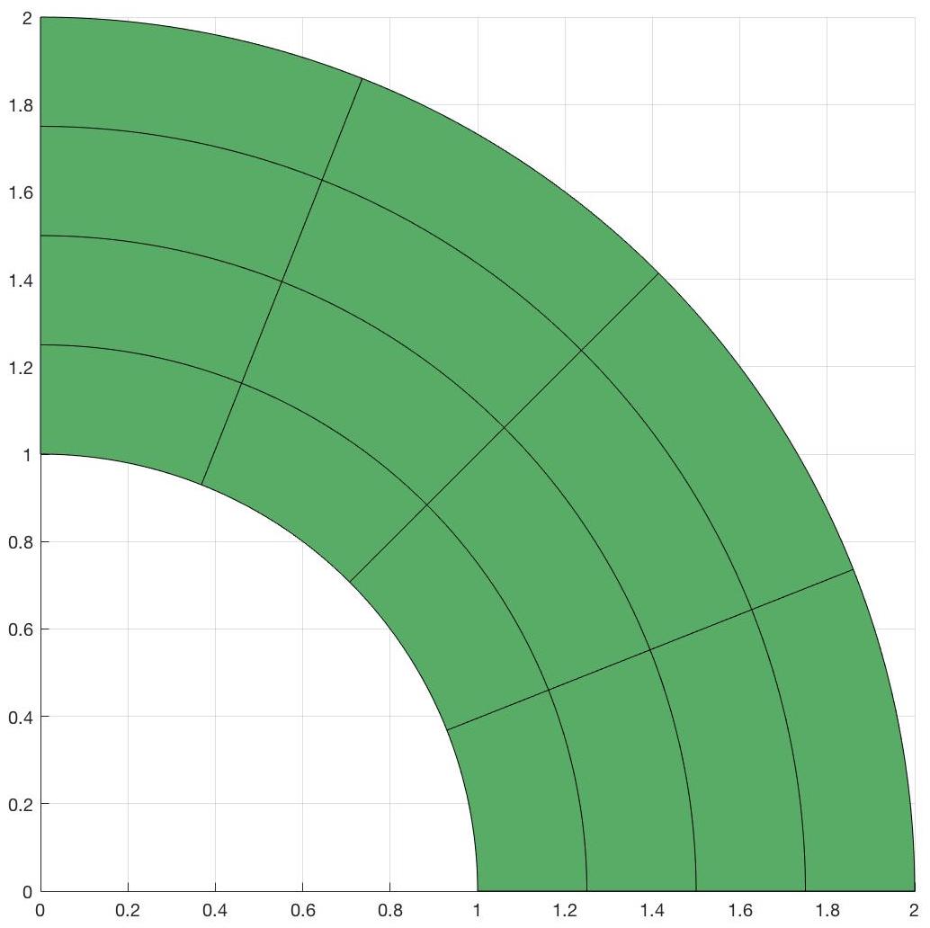
(a)

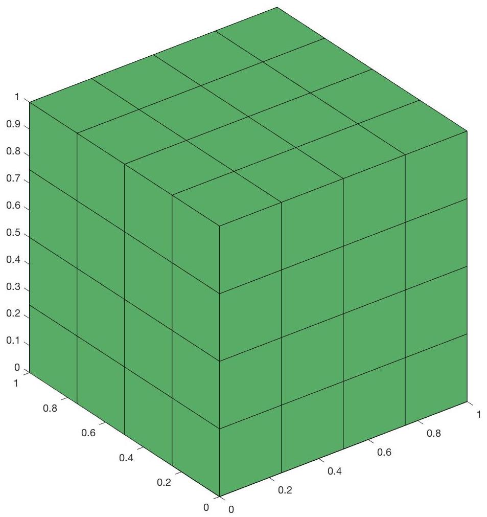
(b)

(c)

Figure 1: Computational domains.

5.1 Orders of convergence.

We perform accuracy tests in a 2D spatial domain since the calculation of the numerical errors on 3D spatial domains is expensive in terms of computational time, when element-wise Gaussian quadrature is adopted. We set $T=1$ and we consider a 2D spatial domain: the quarter of annulus with internal radius equal to 1 and external radius equal to 2 (see Figure LABEL:fig:quarter). The initial and Dirichlet boundary conditions and the source term $f$ are fixed such that the exact solution is $u=-(x^{2}+y^{2}-1)(x^{2}+y^{2}-4)xy^{2}\sin(\pi t)$. We solved the linear system with Matlab direct solver (backslash “ \” operator). Figure LABEL:fig:space-time_error_V0 shows the $\|\cdot\|_{\mathcal{V}_{0}}$ relative errors with splines of degree $p_{s}=p_{t}$ from 2 to 6: the rate of convergence of $O(h^{p_{t}-1})$ confirms the results of Theorem 3. As predicted by the theory, if we increase the degree of spatial B-splines and we set $p_{s}=p_{t}+1$, we can gain an order of convergence. Indeed, Figure LABEL:fig:space-time_error_V0_unbalanced shows that in this case the $\|\cdot\|_{\mathcal{V}_{0}}$ relative errors have order $p_{t}$.

Even if theoretical results do not cover this case, we also analyze in Figures LABEL:fig:space-time_error_L2 and LABEL:fig:space-time_error_H1 the error behaviour for $p_{t}=p_{s}$ in $L^{2}(\Omega\times[0,T])$ and $H^{1}(\Omega\times[0,T])$ norms, respectively. While the $H^{1}$ errors are optimal for every $p_{t}$ considered, i.e. they are of order ${p_{t}}$ for $p_{t}\geq 2$, the orders of convergence in $L^{2}$ norm are optimal and thus equal to $p_{t}+1$, only for $p_{t}\geq 3$. The suboptimal behaviour of the error in $L^{2}$ norm for $p_{t}=p_{s}=2$ is in fact consistent with the Aubin-Nitsche type estimate and with the a-priori error estimates for fourth-order PDEs (see in particular the classical result [42, Theorem 3.7]).

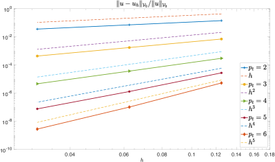
(a)

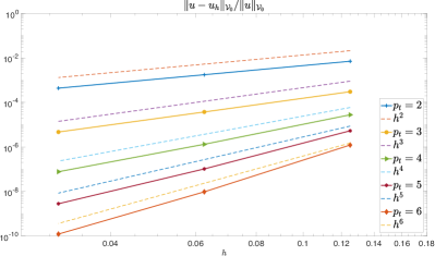
(b)

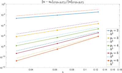
(c)

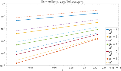
(d)

Figure 2: Relative errors.

5.2 Performance of the preconditioner

To assess the performance of our preconditioning strategy, we set $T=1$ and we focus on two 3D spatial domains $\Omega\subset\mathbb{R}^{3}$, represented in Figure LABEL:fig:cube and Figure LABEL:fig:rev_quarter: the cube and the rotated quarter of annulus, respectively. As a comparison, we also consider as preconditioner for CG the Incomplete Cholesky with zero fill-in (IC(0)) factorization of $\bm{A}$, that is executed by the Matlab routine ichol. Tables 1 and 2 report the number of iterations and the total solving time, that includes the setup time of the preconditioner. The symbol “ * ” is used when the construction of the matrix $\bm{A}$ or its matrix factors go out-of-memory. We force the execution to be sequential and to use only a single computational thread.

As discussed in the previous section, the matrix-vector products of CG are computed in a matrix-free way using its factors as in (30). Matrix $\bm{A}$ is still assembled in order to use the IC(0) preconditioner. In any case, the assembly times are never included in the reported times.

We first consider the domain $\widehat{\Omega}=\Omega=(0,1)^{3}$ (Figure LABEL:fig:cube). Note that in this case we have that $[\bm{P}]_{i,j}=\mathcal{\widehat{P}}(\widehat{B}_{i,\bm{p}},\widehat{B}_{j,\bm{p}})=\mathcal{P}(B_{i,\bm{p}},B_{j,\bm{p}})$. We set homogeneous Dirichlet and zero initial boundary conditions and we fix $f$ such that the exact solution is $u=\sin(\pi x)\sin(\pi y)\sin(\pi z)\sin(t)$.

Table 1 shows the performance of $\bm{P}$ and IC(0) preconditioners in the case $p_{t}=p_{s}$. The number of iterations obtained with $\bm{P}$ are stable w.r.t $p_{t}$ and $n_{sub}$.

Even if the number of iterations of our strategy might be larger than that of IC(0), the overall computational time is significantly lower, up to two orders of magnitude for the problems considered. This is due to the higher setup and application cost of the IC(0) preconditioner.

	$\bm{P}$ + CG  $p_{t}=p_{s}$  Iterations / Time
$n_{sub}$	$p_{t}=2$	$p_{t}=3$	$p_{t}=4$	$p_{t}=5$
8	09 / 0000.06	11 / 0000.07	11 / 000.18	11 / 000.28
16	11 / 0000.27	11 / 0000.69	12 / 001.80	12 / 003.80
32	12 / 0005.10	12 / 0013.37	12 / 027.31	12 / 052.95
64	13 / 0100.09	13 / 0227.93	13 / 458.86	13 / 924.44
128	13 / 2012.94	13 / 4235.96	$\ast$	$\ast$

	IC(0) + CG  $p_{t}=p_{s}$  Iterations / Time
$n_{sub}$	$p_{t}=2$	$p_{t}=3$	$p_{t}=4$	$p_{t}=5$
8	09 / 000.18	07 / 01.69	06 / 014.04	06 / 0080.39
16	22 / 005.01	16 / 45.54	12 / 355.99	10 / 1913.90
32	64 / 157.05	$\ast$	$\ast$	$\ast$

Table 1: Cube domain with $p_{t}=p_{s}$. Performance of $\bm{P}+CG$ (upper table) and of IC(0)+CG (lower table).

Then we consider as computational domain $\Omega$ a quarter of annulus with center in the origin, internal radius 1 and external radius 2, rotated along the axis $y=-1$ by $\pi/2$ (see Figure LABEL:fig:rev_quarter). Boundary data and forcing function are set such that the exact solution is $u=-(x^{2}+y^{2}-1)(x^{2}+y^{2}-4)xy^{2}\sin(z)\sin(t)$.

Table 2 shows the results of CG coupled with $\bm{P}$, $\bm{P}^{\mathbf{G}}$ or IC(0) preconditioner. From the spectral estimates of Theorem 4, we know that the geometry parametrization $\mathbf{G}$, which in this case is not trivial, plays a key-role in the performance of $\bm{P}$. This is confirmed by the results of Table 2: the number of iterations is higher than the ones obtained in the cube domain, where $\mathbf{G}$ is the identity map (see Table 1). However, the inclusion of some geometry information, and thus the use of $\bm{P}^{\mathbf{G}}$ as a preconditioner, improves the performances, as we can see from the middle table of Table 2. Moreover, we show that IC(0) is not competitive neither with $\bm{P}$ nor with $\bm{P}^{\mathbf{G}}$, in terms of computational time.

For the last domain, we analyze the percentage of computation time of a $\bm{P}^{\mathbf{G}}$ application with respect to the overall CG time. The results, reported in Table 3, show that the time spent in the preconditioner application takes only a little amount of the overall solving time. The dominant cost, in this implementation is due to the matrix-vector products of the residual computation, that is the other main operation performed in a CG cycle.

Since we are primarily interested in the preconditioner performance, in Figure 3 we report in a log-log scale the computational times required for the setup and for a single application of $\bm{P}^{\mathbf{G}}$ versus the number of degrees-of-freedom. We see that the setup time is clearly asymptotically proportional to $N_{dof}$, as expected. Remarkably, the single application time grows slower than the expected theoretical cost $O(N_{dof}^{5/4})$; indeed, it grows almost as the optimal rate $O(N_{dof})$, even for the largest problems tested. As already mentioned, this is likely due to the high efficiency of the BLAS level 3 routines that perform the computational core of the application of the preconditioner.

	$\bm{P}$ + CG  $p_{t}=p_{s}$  Iterations / Time
$n_{sub}$	$p_{t}=2$	$p_{t}=3$	$p_{t}=4$	$p_{t}=5$
8	107 / 00000.21	107 / 00000.48	114 / 0001.17	123 / 0002.73
16	126 / 00002.56	128 / 00006.90	133 / 0017.04	135 / 0035.177
32	142 / 00052.77	143 / 00132.24	148 / 0292.53	151 / 0572.84
64	153 / 01056.21	155 / 02415.23	156 / 4956.68	159 / 9906.33
128	164 / 22106.01	166 / 47539.02	$\ast$	$\ast$

	$\bm{P}^{\mathbf{G}}$ + CG  $p_{t}=p_{s}$  Iterations / Time
$n_{sub}$	$p_{t}=2$	$p_{t}=3$	$p_{t}=4$	$p_{t}=5$
8	24 / 0000.09	24 / 00000.13	26 / 0000.37	26 / 0000.60
16	35 / 0000.77	34 / 00001.96	33 / 0004.62	33 / 0009.35
32	42 / 0017.03	41 / 00039.57	40 / 0082.35	41 / 0161.73
64	46 / 0333.20	44 / 00716.03	49 / 1577.55	53 / 3384.08
128	48 / 6767.08	50 / 14814.09	$\ast$	$\ast$

	IC(0) + CG  $p_{t}=p_{s}$  Iterations / Time
$n_{sub}$	$p_{t}=2$	$p_{t}=3$	$p_{t}=4$	$p_{t}=5$
8	11 / 000.17	08 / 01.71	07 / 013.96	06 / 0080.28
16	29 / 005.52	18 / 45.22	14 / 377.47	11 / 1895.55
32	86 / 185.08	$\ast$	$\ast$	$\ast$

Table 2: Rotated quarter domain with $p_{t}=p_{s}$. Performance of $\bm{P}+CG$ (upper table), $\bm{P}^{\mathbf{G}}+CG$ (middle table) and of IC(0)+CG (lower table).

	$\bm{P}^{\mathbf{G}}$
$n_{sub}$	$p_{t}=2$	$p_{t}=3$	$p_{t}=4$	$p_{t}=5$
8	35.86%	20.66%	10.85%	07.05 %
16	17.90%	08.10 %	03.95 %	02.28 %
32	14.25 %	07.35 %	04.05 %	02.49 %
64	17.28 %	08.75 %	04.67 %	02.52 %
128	23.98 %	12.21 %	$\ast$	$\ast$

Table 3: Rotated quarter domain with $p_{t}=p_{s}$. Percentage of computational time of the preconditioner $\bm{P}^{\mathbf{G}}$ application in the overall CG cycle.

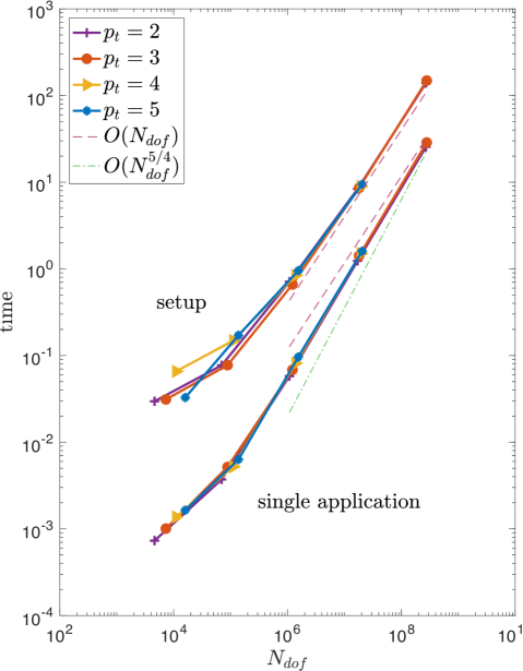
Figure 3: Rotated quarter domain with $p_{t}=p_{s}$. Setup times and single application times of $\bm{P}^{\mathbf{G}}$.

6 Conclusions

In this paper, we have proposed and studied a least-squares method for the heat equation, that allows us to design an innovative preconditioner in the framework of isogeometric analysis. Even though we adopt a global-in-time space-time formulation, based on smooth splines in space and time, the preconditioner $\bm{P}$ that we have presented is highly efficient both in terms of FLOPs and memory, thanks to its matrix representation as suitable sum of Kronecker products, leading to a Sylvester-like problem.

The computational cost of the preconditioner setup is at most $O(N_{dof})$ FLOPs while its application is $O(N_{dof}^{1+1/d})$ FLOPs. In our numerical benchmarks the computational time, for serial single-core execution, is in fact close to $O(N_{dof})$, with no dependence on $p$. The proposed preconditioner $\bm{P}$ is indeed robust with respect to the spline degree and its variant, denoted with $\bm{P}^{\mathbf{G}}$, has a good performance also when the geometry parametrization ${\mathbf{G}}$ of the patch is not trivial.

The storage cost is instead $O(p^{d}N_{s}+N_{dof})$, under the reasonable assumption that $n^{2}_{t}\leq Cp^{d}N_{s}$. We emphasize that is roughly the same storage cost that one would get by discretizing separately in space and time.

Our approach could be coupled with a matrix-free idea (see [36]), and this is expected to further improve the efficiency of the overall method. Everything is well-suited for parallelization: even though in this paper we do not consider parallel implementation, this is a promising research direction for the future.

Appendix A Appendix

A.1 Smooth approximation of $\widehat{\mathcal{V}}_{0}$

In this appendix we prove the density of spaces of smooth functions, with boundary conditions, in suitable Sobolev spaces on the parametric domain. The first result concerns $H^{1}_{0}\cap H^{2}$.

Lemma 6.

Let $Q:=\widehat{\Omega}\times(a,b)$ be an open $(d+1)$-dimensional box. Then, the space $C^{\infty}\left({\overline{Q}}\right)\cap H^{1}_{0}\left({{Q}}\right)$ is dense in $H^{2}\left({{Q}}\right)\cap H^{1}_{0}\left({{Q}}\right)$.

Proof.

Let $w\in H^{2}\left({{Q}}\right)\cap H^{1}_{0}\left({{Q}}\right)$ and $g:=-\Delta w\in L^{2}\left({{Q}}\right)$. Clearly, $w$ solves, in a weak sense,

$$\begin{cases}-\Delta w=g&\text{in ${{Q}}$,}\\ \hskip 14.22636ptw=0&\text{on $\partial{{Q}}$.}\par\end{cases}$$

Let $g_{n}\in C^{\infty}_{0}\left({{Q}}\right)$ such that $g_{n}\to g$ in $L^{2}({{Q}})$ and let $w_{n}\in H^{1}_{0}\left({Q}\right)$ be the weak solution of

$$\begin{cases}-\Delta w_{n}=g_{n}&\text{in ${{Q}}$,}\\ \hskip 14.79541ptw_{n}=0&\text{on $\partial{{Q}}$.}\par\end{cases}$$

Then $w_{n}\to w$ in $H^{2}\left({{Q}}\right)$. Note that $w_{n}$ is defined on ${\overline{Q}}$, vanishes on its boundary $\partial{{Q}}$ and is harmonic in a inner neighborhood of $\partial{{Q}}$ because $g_{n}$ has compact support, thus, employing recursively Schwarz reflection (see, e.g., [18, Exercise 9, Section 2.5] and [10, Remarque 10, Section IX.2]) we can extend $w_{n}$ outside ${\overline{Q}}$, such that this extension is harmonic in a neighborhood of $\partial{{Q}}$. It follows that $w_{n}\in C^{\infty}\left({\overline{Q}}\right)$. ∎

The second result focuses on the space which is needed for our least-squares formulation, that is, $H^{2}$ in space and $H^{1}$ in time, endowed with homogeneous initial and boundary conditions. This is used to show, in Theorem 2, the convergence of our method.

Lemma 7.

Let

$$\widehat{\mathcal{V}}_{0}= \left\{v\in\left[\left(H^{2}({\widehat{\Omega}})\cap H^{1}_{0}({\widehat{\Omega}})\right)\otimes L^{2}(0,1)\right]\cap\left[L^{2}({\widehat{\Omega}})\otimes H^{1}(0,1)\right]\ \text{ s.t. }\ \ v=0\text{ on }{\widehat{\Omega}}\times\{0\}\right\}$$

be a Hilbert space endowed with the norm

$$\|v\|_{\widehat{\mathcal{V}}_{0}}^{2}:=\int_{0}^{1}\|\Delta v(\cdot,\tau)\|_{L^{2}(\widehat{\Omega})}^{2}\,\mathrm{d}\tau+\int_{0}^{1}\|\partial_{\tau}v(\cdot,\tau)\|_{L^{2}(\widehat{\Omega})}^{2}\,\mathrm{d}\tau.$$

Then, the space $C^{\infty}\left([0,1]^{d+1}\right)\cap\widehat{\mathcal{V}}_{0}$ is dense in $\widehat{\mathcal{V}}_{0}$.

Proof.

Consider a given $w\in\widehat{\mathcal{V}}_{0}$ as the solution of a heat problem on the parametric domain $\widehat{\Omega}\times(0,1)=(0,1)^{d+1}$, with datum $g:=(\partial_{t}w-\Delta w)\in L^{2}\left((0,1)^{d+1}\right)$, i.e.

$$\begin{cases}\partial_{t}w-\Delta w\ =\ g\quad&\mbox{in }\ \ \ \hskip 2.84526pt\widehat{\Omega}\times(0,1),\\ w\ =\ 0\quad\quad&\mbox{on }\ \hskip 1.99168pt\partial\widehat{\Omega}\times(0,1),\\ w\ =\ 0\quad&\mbox{in }\ \ \ \ \widehat{\Omega}\times\{0\}.\end{cases}$$ (39)

Let $g_{n}\in C^{\infty}_{0}\left((0,1)^{d+1}\right)$ such that $g_{n}\to g$ in $L^{2}\left((0,1)^{d+1}\right)$ and let $w_{n}$ be the solution of the same heat problem (39) with datum $g_{n}$. Following the proof of Theorem 1 applied in ${\widehat{\Omega}}\times(0,1),$ we get $w_{n}\to w$ in $\widehat{\mathcal{V}}_{0}$ while, by [18, Section 7.1.3, Theorem 6], we also get $w_{n}\in L^{2}({\widehat{\Omega}})\otimes H^{2}(0,1)$.

We use now Lemma 6 to approximate $w_{n}$. Fix $\delta>0$ and consider an extension $z_{n}$ of $w_{n}$ and $z_{n}\in\left[\left(H^{2}({\widehat{\Omega}})\cap H^{1}_{0}({\widehat{\Omega}})\right)\otimes L^{2}(0,1+\delta)\right]\cap\left[L^{2}({\widehat{\Omega}})\otimes H^{2}(0,1+\delta)\right]$ such that $z_{n}(\cdot,1+\delta)=0$. Now observe that $z_{n}$ is a function in $\in H^{2}\left(\widehat{\Omega}\times(0,1+\delta)\right)\cap H^{1}_{0}\left(\widehat{\Omega}\times(0,1+\delta)\right)$, we can then apply Lemma 6 to construct a sequence ${z}_{n,k}\in C^{\infty}\left({[0,1]^{d}}\times[0,1+\delta]\right)\cap H^{1}_{0}\left(\widehat{\Omega}\times(1+\delta)\right)$ converging, as $k\rightarrow\infty$, to $z_{n}$ in the $H^{2}\left(\widehat{\Omega}\times(0,1+\delta)\right)$ norm. The restriction of ${z}_{n,k}$ to $[0,1]^{d+1}$ belongs to the required space $C^{\infty}\left({[0,1]^{d+1}}\right)\cap\widehat{\mathcal{V}}_{0}$ and the sequence converges (as $k\rightarrow\infty$) to $z_{n}$ in the $H^{2}((0,1)^{d+1})$ norm, and thus in the $\widehat{\mathcal{V}}_{0}$-norm. ∎

A.2 A variational formulation equivalent to (13)–(14)

In this appendix, we show that the least-squares space-time functional

$$\mathcal{E}_{LS}(v):=\tfrac{1}{2}\int_{0}^{T}\|\partial_{t}v(\cdot,t)-\Delta v(\cdot,t)-f(\cdot,t)\|^{2}_{L^{2}(\Omega)}\,\mathrm{dt}\quad\forall v\in\mathcal{V}_{0}$$ (40)

that appears in the minimization problem (13), coincides with another space-time functional (A.2) appearing in the theory of gradient flows and curves of maximal slopes (see e.g., [1, 37]).

First, let us introduce the energy $\mathcal{J}:H^{1}_{0}(\Omega)\times[0,T]\to\mathbb{R}$ given by

$$\mathcal{J}(w,t):=\int_{\Omega}\left(\tfrac{1}{2}|\nabla w(\bm{x})|^{2}-f(\bm{x},t)w(\bm{x})\right)\,\mathrm{d}\Omega$$

and assume, for the sake of simplicity, that $f\in H^{1}(0,T;L^{2}(\Omega))=L^{2}(\Omega)\otimes H^{1}(0,T)$. If $w\in H^{1}_{0}(\Omega)\cap H_{\Delta}(\Omega)$ then for all $z\in H^{1}_{0}(\Omega)$ and for all $t\in(0,T)$ by Green’s formula we have

$$\partial_{w}\mathcal{J}(w,t)[z]=\int_{\Omega}\big{(}-\Delta w(\bm{x})-f(\bm{x},t)\big{)}z(\bm{x})\,\mathrm{d}\Omega.$$

Moreover, thanks to the regularity of $f$ we have

$$\partial_{t}\mathcal{J}(w,t)=-\int_{\Omega}w(\bm{x})\partial_{t}f(\bm{x},t)\,\mathrm{d}\Omega.$$

At this point, let us see that the functional $\mathcal{E}_{LS}$ coincides with the following functional defined $\forall v\in\mathcal{V}_{0}$

$$\mathcal{E}(v):= \mathcal{J}(v(\cdot,T),T)+\tfrac{1}{2}\int_{0}^{T}\left(\|\partial_{t}v(\cdot,t)\|^{2}_{L^{2}(\Omega)}+\|\Delta v(\cdot,t)+f(\cdot,t)\|^{2}_{L^{2}(\Omega)}\right)\,\mathrm{dt}\,-\int_{0}^{T}\partial_{t}\mathcal{J}(v(\cdot,t),t)\,\mathrm{dt}.$$

For $v\in\mathcal{V}_{0}$ we know, e.g., by [9, Lemme 3.3], that the energy $t\mapsto\mathcal{J}(v(\cdot,t),t)$ is absolutely continuous and thus

$$\mathcal{J}(v(\cdot,T),T) =\int_{0}^{T}\frac{\mathrm{d}}{\mathrm{d}t}\mathcal{J}(v(\cdot,t),t)\,\mathrm{dt}=\int_{0}^{T}\left(\partial_{w}\mathcal{J}(v(\cdot,t),t)[\partial_{t}v(\cdot,t)]+\partial_{t}\mathcal{J}(v(\cdot,t),t)\right)\mathrm{dt}$$

$$=\int_{0}^{T}\int_{\Omega}\big{(}-\Delta v-f\big{)}\partial_{t}v\,\mathrm{d}\Omega\,\mathrm{dt}-\int_{0}^{T}\int_{\Omega}v\,\partial_{t}f\,\mathrm{d}\Omega\,\mathrm{dt}\,.$$

Then, we can re-write the least-squares functional (40) as follows:

$$\mathcal{E}_{LS}(v) =\tfrac{1}{2}\int_{0}^{T}\left(\|\partial_{t}v(\cdot,t)\|^{2}_{L^{2}(\Omega)}+\|\Delta v(\cdot,t)+f(\cdot,t)\|^{2}_{L^{2}(\Omega)}\right)\,\mathrm{dt}-\int_{0}^{T}\int_{\Omega}(\Delta v+f)\partial_{t}v\,\mathrm{d}\Omega\,\mathrm{dt}$$ (41)

$$=\mathcal{J}(v(\cdot,T),T)+\tfrac{1}{2}\int_{0}^{T}\left(\|\partial_{t}v(\cdot,t)\|^{2}_{L^{2}(\Omega)}+\|\Delta v(\cdot,t)+f(\cdot,t)\|^{2}_{L^{2}(\Omega)}\right)\,\mathrm{dt}\,-\int_{0}^{T}\partial_{t}\mathcal{J}(v(\cdot,t),t)\,\mathrm{dt}$$

$$=\mathcal{E}(v).$$

As a consequence, the representation (29) in the discrete space $\mathcal{V}_{h,0}$ holds also in the space $\mathcal{V}_{0}$, moreover, the bilinear form (15) turns out to be the Euler-Lagrange equation of the functional (A.2).

A.3 Separation of variables algorithm

After approximating each function by piecewise constants, (38) becomes

$$\left[\mathfrak{C}^{(k)}\right]_{i_{1},\dots,i_{d+1}}\approx[{\bm{\mu}}^{(1)}]_{i_{1}}\dots[\bm{\mu}^{(k-1)}]_{i_{k-1}}[\bm{\omega}^{(k)}]_{i_{k}}[\bm{\mu}^{(k+1)}]_{i_{k+1}}\dots[\bm{\mu}^{(d+1)}]_{i_{d+1}},$$ (42)

where, denoting by $\mathbb{R}_{+}$ the set of strictly positive real numbers, the tensors $\mathfrak{C}^{(k)}\in\mathbb{R}_{+}^{n_{1}\times\dots\times n_{d+1}}$ are given and $\bm{\mu}^{(k)},\bm{\omega}^{(k)}\in\mathbb{R}_{+}^{n_{k}}$, $k=1,\ldots,d+1$, are unknown vectors to be computed. In our case, $n_{1},\ldots,n_{d}$ are the number of elements in each space direction and $n_{d+1}$ the number of elements in time, and we construct $\mathfrak{C}^{(k)}\in\mathbb{R}_{+}^{n_{1}\times\dots\times n_{d+1}}$ by interpolating $c_{k}$ in the element barycenters.

In order to compute the approximation (42), we aim at finding $\bm{\mu}^{(k)},\bm{\omega}^{(k)}\in\mathbb{R}_{+}^{n_{k}}$ for $k=1,\dots,d+1$, that minimize the functional

$$\left[\bm{\chi}^{(k)},\bm{\psi}^{(k)}\ \right]_{k=1,\dots,d+1}\longmapsto\ \max_{\begin{subarray}{c}i_{k}=1,\dots,n_{k};\\ k=1,\dots,d+1\end{subarray}}\left\{\left|\log\left(\frac{[\mathfrak{C}^{(k)}]_{i_{1},\dots,i_{d+1}}}{[\bm{\chi}^{(1)}]_{i_{1}}\dots[\bm{\chi}^{(k-1)}]_{i_{k-1}}[\bm{\psi}^{(k)}]_{i_{k}}[\bm{\chi}^{(k+1)}]_{i_{k+1}}\dots[\bm{\chi}^{(d+1)}]_{i_{d+1}}}\right)\right|\right\}.$$

Equivalently, we look for $\bm{\mu}^{(k)},\bm{\omega}^{(k)}\in\mathbb{R}_{+}^{n_{k}}$ for $k=1,\dots,d+1$, such that the minimum and maximum values of the ratio

$$\frac{[\mathfrak{C}^{(k)}]_{i_{1},\dots,i_{d+1}}}{[\bm{\mu}^{(1)}]_{i_{1}}\dots[\bm{\mu}^{(k-1)}]_{i_{k-1}}[\bm{\omega}^{(k)}]_{i_{k}}[\bm{\mu}^{(k+1)}]_{i_{k+1}}\dots[\bm{\mu}^{(d+1)}]_{i_{d+1}}},$$

for $i_{k}=1,\dots,n_{k};\;k=1,\dots,d+1$, are as close as possible to 1 (in the logarithmic sense).

Algorithm 2 computes an approximate solution of the above optimization problem. This algorithm generalizes the one used in [47] which is focused on the case of two variables, i.e. it computes the approximations

$$\left[\mathfrak{C}^{(1)}\right]_{i_{1},i_{2}}\approx[\bm{\omega}^{(1)}]_{i_{1}}[{\bm{\mu}}^{(2)}]_{i_{2}},\qquad\left[\mathfrak{C}^{(2)}\right]_{i_{1},i_{2}}\approx[{\bm{\mu}}^{(1)}]_{i_{1}}[\bm{\omega}^{(2)}]_{i_{2}}.$$

Note that in this case the two approximation problems are completely decoupled, so they can be solved independently. As in [47], in all our tests we set $maxit=2$.

Algorithm 2 Separation of variables

1:Initialize $\bm{\mu}^{(l)}=\bm{\omega}^{(l)}=\mathbf{1}_{n_{l}}$ for $l=1,\dots,d+1$.

2:for  $iter=1\dots maxit$ do

3:     for $k=1,\dots,{d+1}$ do

4:         Compute $\mathfrak{V}^{(k)}\in\mathbb{R}^{n_{1}\times\dots\times n_{d+1}}$ s.t.

5:          $\left[\mathfrak{V}^{(k)}\right]_{i_{1},\dots,i_{d+1}}=\frac{[\mathfrak{C}^{(k)}]_{i_{1},\dots,i_{d+1}}}{[\bm{\mu}^{(1)}]_{i_{1}}\dots[\bm{\mu}^{(k-1)}]_{i_{k-1}}[\bm{\mu}^{(k+1)}]_{i_{k+1}}\dots[\bm{\mu}^{({d+1})}]_{i_{d+1}}}.$

6:         for $j=1,\dots,n_{k}$ do

7:              Compute $m=\min\left\{\mathfrak{V}^{(k)}_{i_{1},\dots,i_{k-1},j,i_{k+1},\dots i_{{d+1}}}\text{ s.t. }i_{l}=1,\dots,n_{l};l=1,\dots,{d+1}\text{ and }l\neq k\right\}.$

8:              Compute $M=\max\left\{\mathfrak{V}^{(k)}_{i_{1},\dots,i_{k-1},j,i_{k+1},\dots i_{{d+1}}}\text{ s.t. }i_{l}=1,\dots,n_{l};l=1,\dots,{d+1}\text{ and }l\neq k\right\}.$

9:              Update $[\bm{\omega}^{(k)}]_{j}=\sqrt{mM}.$

10:         end for

11:     end for

12:     for $k=1,\dots,{d+1}$ do

13:         for $l=1,\dots,{d+1}$ do

14:              if $l\neq k$ then

15:                  Compute $\mathfrak{W}^{(k,l)}\in\mathbb{R}^{n_{1}\times\dots\times n_{d+1}}$ s.t.

16:          $\left[\mathfrak{W}^{(k,l)}\right]_{i_{1},\dots,i_{d+1}}=\frac{[\mathfrak{C}^{(k)}]_{i_{1},\dots,i_{d+1}}[\bm{\mu}^{(l)}]_{i_{l}}}{[\bm{\mu}^{(1)}]_{i_{1}}\dots[\bm{\mu}^{(k-1)}]_{i_{k-1}}[\bm{\omega}^{(k)}]_{i_{k}}[\bm{\mu}^{(k+1)}]_{i_{k+1}}\dots[\bm{\mu}^{({d+1})}]_{i_{d+1}}}.$

17:              end if

18:         end for

19:         Compute $\mathfrak{Y}\in\mathbb{R}^{n_{1}\times\dots\times n_{d+1}}$ s.t. $[\mathfrak{Y}]_{i_{1},\dots,i_{n_{d+1}}}=\min\left\{[\mathfrak{W}^{(k,l)}]_{i_{1},\dots,i_{n_{d+1}}}\text{ s.t. }l=1,\dots,{d+1}\text{ and }l\neq k\right\}$

20:         Compute $\mathfrak{Z}\in\mathbb{R}^{n_{1}\times\dots\times n_{d+1}}$ s.t. $[\mathfrak{Z}]_{i_{1},\dots,i_{n_{d+1}}}=\max\left\{[\mathfrak{W}^{(k,l)}]_{i_{1},\dots,i_{n_{d+1}}}\text{ s.t. }l=1,\dots,{d+1}\text{ and }l\neq k\right\}$

21:         for $j=1,\dots,n_{k}$ do

22:              Compute $m=\min\left\{[\mathfrak{Y}]_{i_{1},\dots,i_{k-1},j,i_{k+1},\dots i_{{d+1}}}\text{ s.t. }i_{l}=1,\dots,n_{l};l=1,\dots,{d+1}\text{ and }l\neq k\right\}.$

23:              Compute $M=\max\left\{[\mathfrak{Z}]_{i_{1},\dots,i_{k-1},j,i_{k+1},\dots i_{{d+1}}}\text{ s.t. }i_{l}=1,\dots,n_{l};l=1,\dots,{d+1}\text{ and }l\neq k\right\}.$

24:              Update $[\bm{\mu}^{(k)}]_{j}=\sqrt{mM}.$

25:         end for

26:     end for

27:end for

References

- [1] L. Ambrosio, N. Gigli, and G. Savaré. Gradient flows: in metric spaces and in the space of probability measures. Springer Science & Business Media, 2008.
- [2] J.-P. Aubin. Applied functional analysis. John Wiley & Sons, New York-Chichester-Brisbane, 1979. Translated from the French by Carole Labrousse, With exercises by Bernard Cornet and Jean-Michel Lasry.
- [3] L. Beirão da Veiga, A. Buffa, G. Sangalli, and R. Vázquez. Mathematical analysis of variational isogeometric methods. Acta Numerica, 23:157–287, 2014.
- [4] L. Beirão da Veiga, D. Cho, and G. Sangalli. Anisotropic NURBS approximation in isogeometric analysis. Computer Methods in Applied Mechanics and Engineering, 209:1–11, 2012.
- [5] B. C. Bell and K. S. Surana. A space–time coupled -version least-squares finite element formulation for unsteady fluid dynamics problems. International journal for numerical methods in engineering, 37(20):3545–3569, 1994.
- [6] B. C. Bell and K. S. Surana. A space-time coupled -version least squares finite element formulation for unsteady two-dimensional Navier–Stokes equations. International journal for numerical methods in engineering, 39(15):2593–2618, 1996.
- [7] P. B. Bochev and M. D. Gunzburger. Least-squares finite element methods, volume 166. Springer Science & Business Media, 2009.
- [8] A. Bressan and E. Sande. Approximation in FEM, DG and IGA: A Theoretical Comparison. arXiv preprint arXiv:1808.04163, 2018.
- [9] H. Brézis. Opérateurs maximaux monotones et semi-groupes de contractions dans les espaces de Hilbert. 5, 1973. North-Holland Mathematics Studies, No. 5. Notas de Matemática (50).
- [10] H. Brezis. Analyse fonctionnelle. Théorie et applications. Collection Mathématiques Appliquées pour la Maîtrise. Masson, Paris, 1983.
- [11] N. Collier, L. Dalcin, D. Pardo, and V. M. Calo. The cost of continuity: performance of iterative solvers on isogeometric finite elements. SIAM Journal on Scientific Computing, 35(2):A767–A784, 2013.
- [12] J. A. Cottrell, T. J. R. Hughes, and Y. Bazilevs. Isogeometric analysis: toward integration of CAD and FEA. John Wiley & Sons, 2009.
- [13] J. A. Cottrell, T. J. R. Hughes, and A. Reali. Studies of refinement and continuity in isogeometric structural analysis. Computer Methods in Applied Mechanics and Engineering, 196(41):4160–4183, 2007.
- [14] C. De Boor. A practical guide to splines (revised edition). Applied Mathematical Sciences. Springer, Berlin, 2001.
- [15] M. O. Deville, P. F. Fischer, and E. H. Mund. High-order methods for incompressible fluid flow. Cambridge University Press, 2002.
- [16] C. A. Dorao and H. A. Jakobsen. A parallel time–space least-squares spectral element solver for incompressible flow problems. Applied mathematics and computation, 185(1):45–58, 2007.
- [17] J. A. Evans, Y. Bazilevs, I. Babuška, and T. J. R. Hughes. -widths, sup-infs, and optimality ratios for the -version of the isogeometic finite element method. Comput. Methods Appl. Mech. Engrg., 198:1726–1741, 2009.
- [18] L. C. Evans. Partial Differential equations. American Mathematical Society, Berlin, 2010.
- [19] I. Fried. Finite-element analysis of time-dependent phenomena. AIAA Journal, 7(6):1170–1173, 1969.
- [20] M. J. Gander. 50 years of time parallel time integration. In Multiple Shooting and Time Domain Decomposition Methods, pages 69–113. Springer, 2015.
- [21] P. Grisvard. Elliptic problems in nonsmooth domains, volume 69. SIAM, 2011.
- [22] J. H. Nguyen and Reynen. A space-time least-square finite element scheme for advection-diffusion equations. Computer Methods in Applied Mechanics and Engineering, 42(3):331–342, 1984.
- [23] C. Hofer, U. Langer, and M. Neumüller. Robust Preconditioning for Space-Time Isogeometric Analysis of Parabolic Evolution Problems. arXiv preprint arXiv:1802.09277, 2018.
- [24] T. J. R. Hughes, J. A. Cottrell, and Y. Bazilevs. Isogeometric analysis: CAD, finite elements, NURBS, exact geometry and mesh refinement. Computer Methods in Applied Mechanics and Engineering, 194(39):4135–4195, 2005.
- [25] J. C. Bruch Jr and G. Zyvoloski. Transient two-dimensional heat conduction problems solved by the finite element method. International Journal for Numerical Methods in Engineering, 8(3):481–494, 1974.
- [26] T. G. Kolda and B. W. Bader. Tensor decompositions and applications. SIAM review, 51(3):455–500, 2009.
- [27] A. M. Kvarving and E. M. Rønquist. A fast tensor-product solver for incompressible fluid flow in partially deformed three-dimensional domains: Parallel implementation. Computers & Fluids, 52:22–32, 2011.
- [28] O. A. Ladyzhenskaja and N. N. Ural’ceva. Équations aux dérivées partielles de type elliptique. Dunod, 1968.
- [29] U. Langer, S. E. Moore, and M. Neumüller. Space-time isogeometric analysis of parabolic evolution problems. Computer Methods in Applied Mechanics and Engineering, 306:342 – 363, 2016.
- [30] U. Langer, M. Neumüller, and I. Toulopoulos. Multipatch space-time isogeometric analysis of parabolic diffusion problems. In International Conference on Large-Scale Scientific Computing, pages 21–32. Springer, 2017.
- [31] R. E. Lynch, J. R. Rice, and D. H. Thomas. Direct solution of partial difference equations by tensor product methods. Numerische Mathematik, 6(1):185–199, 1964.
- [32] M. Montardini, G. Sangalli, and M. Tani. Robust isogeometric preconditioners for the Stokes system based on the Fast Diagonalization method. Computer Methods in Applied Mechanics and Engineering, 338:162 – 185, 2018.
- [33] J. T. Oden. A general theory of finite elements. I. Topological considerations. International Journal for Numerical Methods in Engineering, 1(2):205–221, 1969.
- [34] J. T. Oden. A general theory of finite elements. II. Applications. International Journal for Numerical Methods in Engineering, 1(3):247–259, 1969.
- [35] G. Sangalli and M. Tani. Isogeometric preconditioners based on fast solvers for the Sylvester equation. SIAM Journal on Scientific Computing, 38(6):A3644–A3671, 2016.
- [36] G. Sangalli and M. Tani. Matrix-free weighted quadrature for a computationally efficient isogeometric k-method. Computer Methods in Applied Mechanics and Engineering, 338:117 – 133, 2018.
- [37] F. Santambrogio. Euclidean, metric, and Wasserstein gradient flows: an overview. Bulletin of Mathematical Sciences, 7(1):87–154, 2017.
- [38] C. Schwab and R. Stevenson. Space-time adaptive wavelet methods for parabolic evolution problems. Mathematics of Computation, 78(267):1293–1318, 2009.
- [39] F. Shakib and T. J. R. Hughes. A new finite element formulation for computational fluid dynamics: IX. Fourier analysis of space-time Galerkin/least-squares algorithms. Computer Methods in Applied Mechanics and Engineering, 87(1):35–58, 1991.
- [40] L. Sorber, M. Van Barel, and L. De Lathauwer. Tensorlab v2. 0. Available online, URL: www.tensorlab.net, 2014.
- [41] O. Steinbach. Space-time finite element methods for parabolic problems. Computational methods in applied mathematics, 15(4):551–566, 2015.
- [42] G. Strang and G. J. Fix. An analysis of the finite element method, volume 212. Prentice-hall Englewood Cliffs, NJ, 1973.
- [43] L. P. Franca T. J. R. Hughes and G. M. Hulbert. A new finite element formulation for computational fluid dynamics: VIII. The Galerkin/least-squares method for advective-diffusive equations. Computer Methods in Applied Mechanics and Engineering, 73(2):173–189, 1989.
- [44] K. Takizawa, T. E. Tezduyar, A. Buscher, and S. Asada. Space–time fluid mechanics computation of heart valve models. Computational Mechanics, 54(4):973–986, 2014.
- [45] K. Takizawa, T. E. Tezduyar, Y. Otoguro, T. Terahara, T. Kuraishi, and H. Hattori. Turbocharger flow computations with the space–time isogeometric analysis (ST-IGA). Computers & Fluids, 142:15–20, 2017.
- [46] R. Vázquez. A new design for the implementation of isogeometric analysis in Octave and Matlab: GeoPDEs 3.0. Computers & Mathematics with Applications, 72(3):523–554, 2016.
- [47] E. L. Wachspress. Generalized ADI preconditioning. Computers & mathematics with applications, 10(6):457–461, 1984.