Frequency-Dependent Core Shifts in Ultracompact Quasars

Abstract

Results of a pilot project with the participation of the “Kvazar-KVO” radio interferometry array in observations carried out with the European VLBI Network are presented. The aim of the project was to conduct and analyze multi-frequency (1.7, 2.3, 5.0, 8.4 GHz) observations of the parsec-scale jets of 24 active galactic nuclei. Three observing sessions were successfully carried out in October 2008. Maps of the radio intensity distributions have been constructed in all four frequencies using phase referencing. A method for measuring the frequency-dependent shift of the position of the VLBI core by applying relative astrometry to observations of close triplets of radio sources has been developed. The fundamental possibility of detecting core shifts in ultra-compact sources for which traditional methods based on the achromatic positions of optically thin regions of the jet are not suitable is demonstrated. The conditions for successful measurement of this shift are discussed; these are determined by the closeness of the calibrator used, the effective resolution of the system, the quality of the filling of the $uv$ plane, the relative orientations of the jets in the triplets, and the brightnesses of the sources.

1 INTRODUCTION

In images of extragalactic relativistic jets obtained using Very Long Baseline Interferometry (VLBI), the “core” is the name given to the compact, bright feature at the visible base of the jet. The position of the core is determined by absorption in the radiating plasma (synchrotron self-absorption) or in the ambient material Blandford and Königl (1979); Königl (1981); Lobanov (1998). At any given observing frequency $\nu$, the core is located in the region of the jet with optical depth $\tau(\nu)\approx 1$, leading to a shift in the absolute position of the core $r_{\text{core}}\propto\nu^{-1/k_{\text{r}}}$ Lobanov (1998). In the case of synchrotron self-absorption with equipartition between the energy densities of the relativistic particles and the magnetic field, $k_{\text{r}}=1$ Blandford and Königl (1979). However, in the presence of external absorption or gradients in the density and pressure, $k_{\text{r}}$ can differ from unity Lobanov (1998).

The apparent shifts of the cores of active galactic nuclei (AGNs) have direct astrophysical and astrometric applications in relation to compact radio sources. This effect can be used to estimate various physical parameters of compact relativistic jets. At the same time, the shift of the core with frequency can influence measurements and estimates based on multi-frequency VLBI observations: (1) the construction of spectral-index maps Lobanov (1998); Kovalev et al. (2008), (2) measurements of Faraday rotation Hovatta et al. (2012); Kravchenko et al. (2016, 2017), (3) astrometric and geophysical measurements at 4 and 13 cm Ma et al. (1998); Petrov et al. (2009), and (4) comparison of radio and optical coordinate systems Petrov and Kovalev (2017a); Kovalev et al. (2017); Petrov and Kovalev (2017b).

Understanding and taking into account the effects of absorption in such investigations requires systematic studies of core shifts for a representative sample of compact radio sources, in particular, those used for astrometric applications. To achieve this, we organized a pilot experiment on the European VLBI network (EVN), with the following aims: measuring the core shifts of ultracompact quasars via relative astrometry for selected triplets of sources, comparison with the results obtained for traditional methods based on comparison of optically thin parts of the jets observed at different frequencies, gaining experience in the organization of larger-scale astrometric measurements of core shifts in the future, testing the participation of telescopes in the Russian “Kvazar-KVO” array in EVN observations and estimating the gain provided by this participation.

2 OBSERVATIONS AND DATA REDUCTION

2.1 Source Sample

We selected eight ultracompact extragalactic radio sources for these observations, meeting the following criteria: (1) that the source be included in the main list of objects in the catalog of the International Celestial Reference Frame (ICRF) Ma et al. (1998); (2) that the structure index of the source be equal to 1 or 2 Ma et al. (1998), i.e., that the source structure be dominated by the core; (3) that the maximum correlated spectral flux density of the source at 8 GHz exceeds 1.2 Jy. Based on these criteria, we also added the source 1749+096, which is the most compact and bright of the candidate ICRF sources Ma et al. (1998). We also selected two phase calibrators at angular separations of no more than $4^{\circ}$ for each of these sources.

2.2 EVN Observations

Observations of our targets were carried out on the EVN in three 12-hour sessions during October 2008: October 19–20 at S and X bands (central frequencies 2.27 and 8.38 GHz), October 22–23 at C band (4.97 GHz), and October 29–30 at L band (1.66 GHz). At each frequency, we recorded eight frequency channels (so-called IFs), each with a bandwidth of 8 GHz. Both right- and left-circular polarizations were recorded in L and C bands, while only right-circular polarization was recorded in S and X bands. The aggregate bit rate was 512 Mbits/s. The data were correlated at the Joint Institute for VLBI in Europe (JIVE).

Three 32-m telescopes of the Russian “Kvazar-KVO” VLBI network took part in these EVN observations, appreciably improving the $uv$ coverage in the East–West direction (see Section 2.6). However, the failure of the Hartebeesthoek telescope in South Africa significantly limited the North–South resolution of the interferometric array. Unfortunately, this had a very substantial effect on the accuracy of the astrometric measurements, since the baselines to Hartebeesthoek would have provided the highest angular resolution in the resulting data.

2.3 Data Reduction

The preliminary reduction of the data was carried out in the AIPS package Greisen (2003), and included the following steps: removal of bad data based on information received from the telescopes and a visual inspection of the data; application of phase corrections related to the passage of the radio signal through the ionosphere, carried out using the task TECOR; calibration of the amplitudes using system temperatures and gain curves measured at the telescopes using the task APCAL; preliminary calibration of the phases using a global fringe-fitting procedure (the task FRING). Independent solutions for the group delays and fringe frequencies were found for each frequency channel (IF). Corrections for the shape of the complex passband were applied using the task BPASS. Further, the task SPLIT was used to apply all the derived corrections to the data, average over frequency within each IF, and export the $uv$ data in a format suitable for the subsequent analysis.

Maps for all the sources were constructed using the CLEAN algorithm realized in the Difmap package Shepherd (1997). Global amplitude corrections were obtained for each frequency channel and each antenna by comparing the total intensity CLEAN model with the initial calibrated data. The resulting corrections were averaged over all the sources. Amplitude corrections ${>}10\%$ were then applied to the input data using the task CLCOR in AIPS.

The final step in the reduction of the data in AIPS was realizing a phase-referencing regime relating the phases for the weaker sources in each triplet to those of a calibrator. We chose the brightest, most compact source in each triplet as the phase calibrator. Further, we found a phase solution for each such calibrator using the task FRING, taking into account the source structure, which was then applied to both the data for the calibrator itself and the data for the two other sources in the triplet.

2.4 Reconstruction of the VLBI Maps

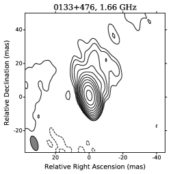
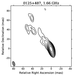
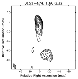
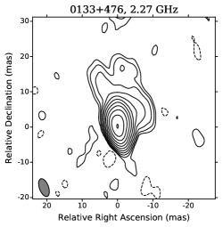
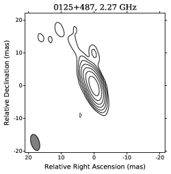
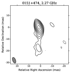
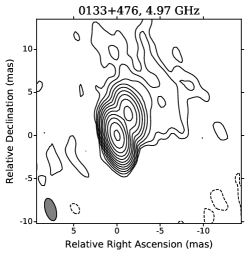
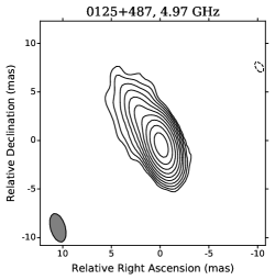
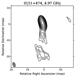
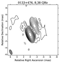
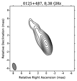
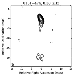
Figure 9: Total-intensity maps of all the target sources made with natural weighting. The first contour corresponds to three times the root-mean-square residual noise.

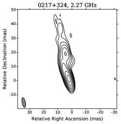
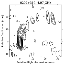
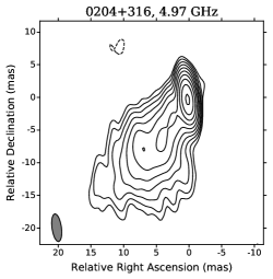
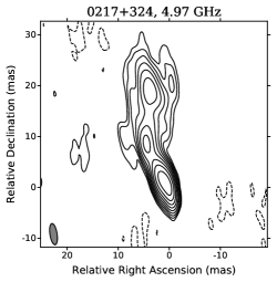
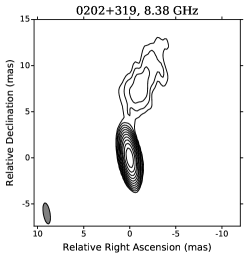
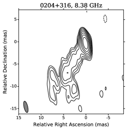
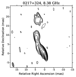
Figure 9: Continued.

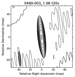
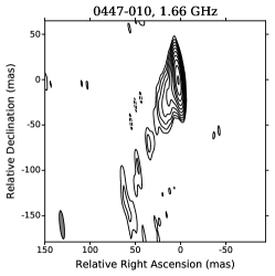
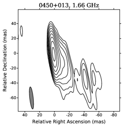
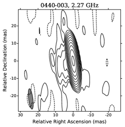
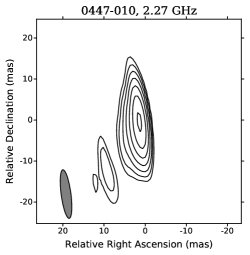
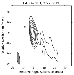
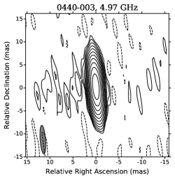
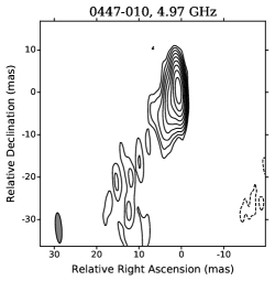
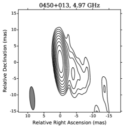
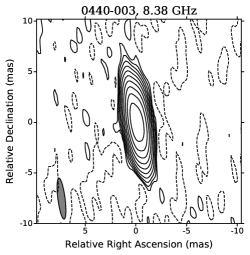
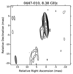
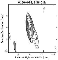
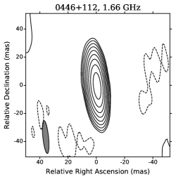
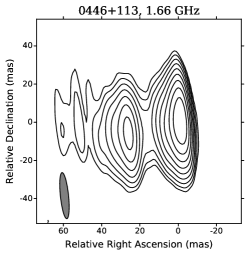
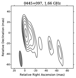
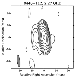
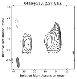
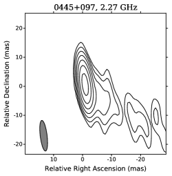
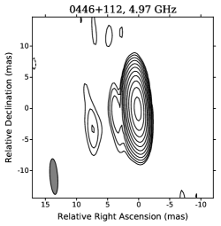
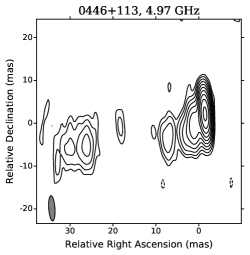
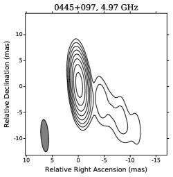
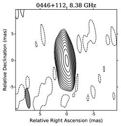
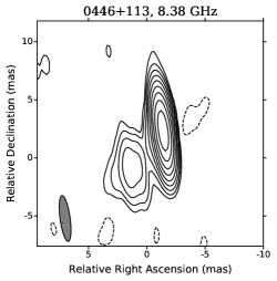
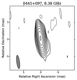
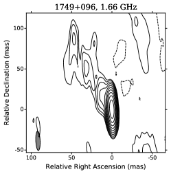
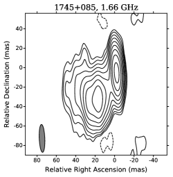
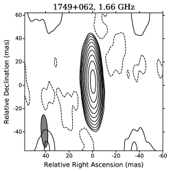
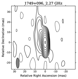
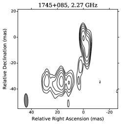
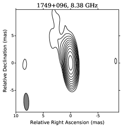
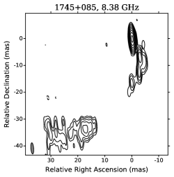
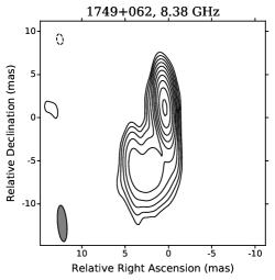
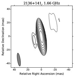
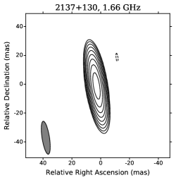
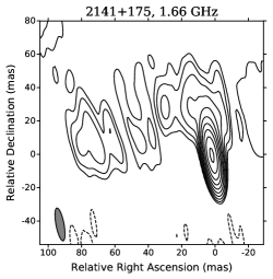
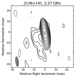
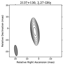
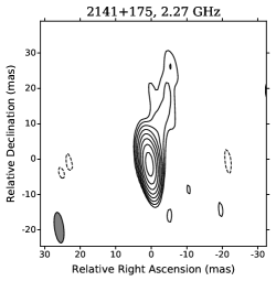
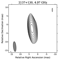
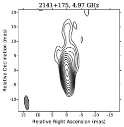
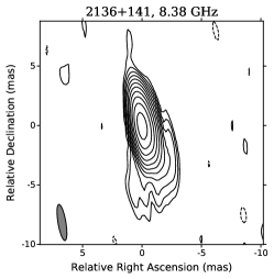
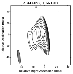
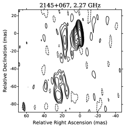
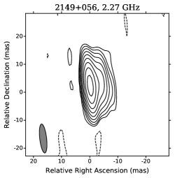
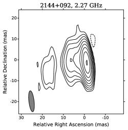
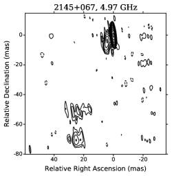
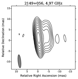
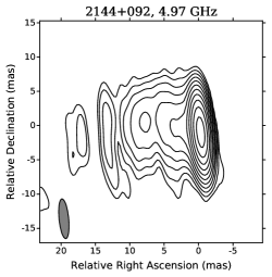
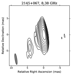
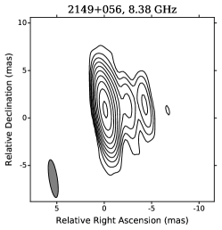
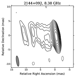
Figure 9: Continued.

The final VLBI maps for the 24 target sources obtained using natural weighting of the data are presented in Fig. 9. Contour maps at 1.7, 2.3, 5.0, and 8.4 GHz are presented for each source. The dynamic ranges of these maps, defined as the ratio of the intensity peak to the noise level in the map, vary from $10^{3}$ for weak sources to $10^{4}$ for the brightest sources at 1.7, 5.0, and 8.4 GHz. The dynamic ranges of the maps at 2.3 GHz are lower, especially for sources weaker than 1 Jy, since the phased Westerbork Synthesis Radio Telescope — one of the most sensitive elements of the EVN — did not take part in the observations at this frequency. The typical noise level of the reconstructed images is 0.3 mJy/beam.

The parameters of the VLBI maps are summarized in Table LABEL:tab:maps, namely, the source name, central frequency of the synthesized image in GHz, peak intensity in mJy/beam, residual noise level in mJy/beam, total flux in mJy, determined as the sum of all CLEAN components, major and minor axes corresponding to the full-width at half-maximum of the restoring beam in milliarcseconds (mas), and the position angle of the beam in degrees.

2.5 Modeling of the Sources

In order to determine the position of the core in the map, we modeled the brightness distribution for each source using a set of circular Gaussian components. The model was fit to the data in the spatial-frequency domain using the Difmap program via $\chi^{2}$ minimization. The number of components was chosen to be the minimum necessary to describe all significant detected elements of the source structure at a given frequency (usually three to six).

2.6 Importance of the Kvazar-KVO Telescopes for the EVN Results

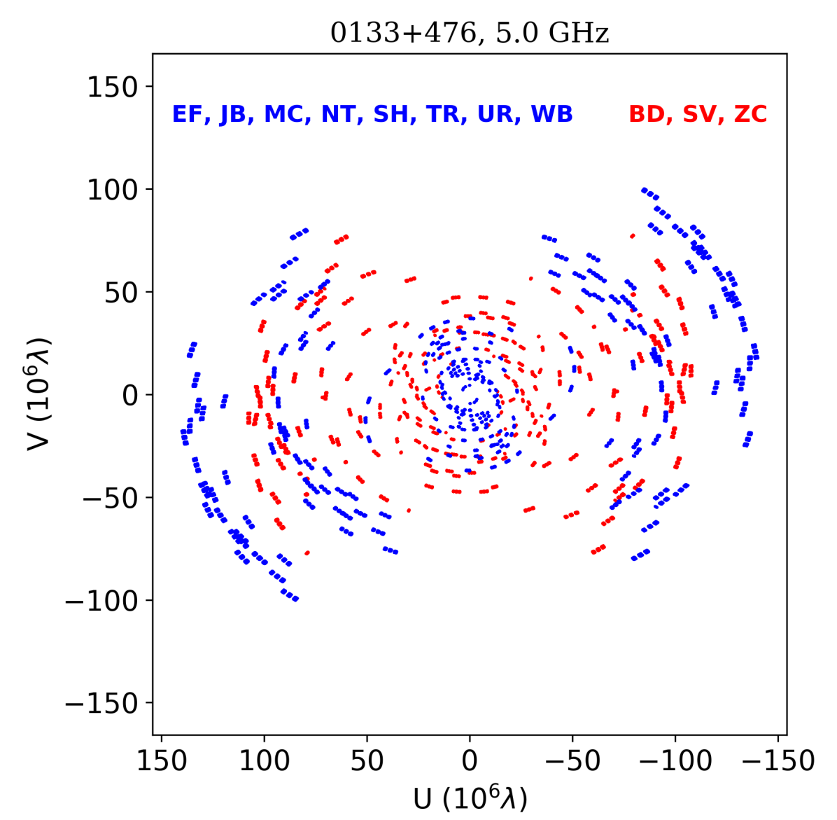
Figure 1: Example of $uv$-coverage for 0133+476 at 5 GHz. The red points denote projected baselines involving Kvazar-KVO telescopes and the blue points show the remaining projected baselines.

Figure 1 shows that the telescopes of the Russian Kvazar–KVO array appreciably improve the filling of the $uv$ plane for the EVN observations, especially at medium-length baselines. The participation of three Kvazar-KVO antennas together with the eight EVN stations increases the number of baselines by about a factor of two, enhancing the reliability of the image reconstruction and appreciably lowering the noise level in the maps. To estimate the contribution made to the data from the Kvazar telescopes, we carried out all the data reduction a second time excluding the Badary, Zelenchuk, and Svetloe telescopes and constructed images of the three sources 0125+487, 0133+476, and 0151+474 at all frequencies. We chose sources with relatively high declinations for this analysis in order to reduce the influence of the poor $uv$-coverage in the North–South direction. Figure 2 compares the residual noise levels in the images reconstructed with and without the Kvazar telescopes. In the latter case, the residual noise level in the images is about 30$\%$ higher, on average. The residual noise in the L, C, and X-band images of 0151+474 remained practically the same. The absence of such additional interferometric baselines is especially important when constructing images of weak sources, whose extended structure may not be detected due to insufficient sensitivity.

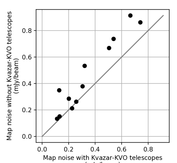
Figure 2: Mean residual noise level in the images constructed with and without the Kvazar–KVO telescopes. The median noise levels are 0.28 and 0.36 mJy/beam, respectively.

2.7 Phase Calibration

The phase of the visibility function at the correlator output is the sum of contributions from various effects:

$$\varphi=\varphi_{\text{struct}}+\varphi_{\text{pos}}+\varphi_{\text{atmo}}+\varphi_{\text{inst}}\,,$$

where $\varphi_{\text{struct}}$ is the phase associated with the source structure, $\varphi_{\text{pos}}$ the phase associated with the position of the source coordinates relative to the phase center, $\varphi_{\text{atmo}}$ the phase due to the atmosphere (ionosphere and troposphere), and $\varphi_{\text{inst}}$ the phase due to delays in the apparatus and imperfection of the frequency standards.

The terms $\varphi_{\text{struct}}$ and $\varphi_{\text{pos}}$ are determined by the source and the terms $\varphi_{\text{atmo}}$ and $\varphi_{\text{inst}}$ by the telescopes and equipment used. The global fringe-fitting minimizes the phase when it introduces global corrections for the antenna phases. Thus, the sum $\varphi_{\text{atmo}}+\varphi_{\text{inst}}+\varphi_{\text{pos}}$ is determined. There remains only the term $\varphi_{\text{struct}}$, which depends on the projected baselines ($uv$ points).

After calibration with the phase calibrator, the phase of the target source will be

$$\varphi^{t}=\varphi_{\text{struct}}^{\text{t}}+(\varphi_{\text{pos}}^{\text{t}}-\varphi_{\text{pos}}^{\text{c}})+(\varphi_{\text{atmo}}^{\text{t}}-\varphi_{\text{atmo}}^{\text{c}})\\ {}+(\varphi_{\text{inst}}^{\text{t}}-\varphi_{\text{inst}}^{\text{c}})\,.$$ (1)

Here, the subscript “c” denotes the calibrator and the subscript “t” the target. The term $\varphi_{\text{struct}}^{\text{c}}$ takes into account the model for the calibrator obtained during our imaging. The term $\varphi_{\text{inst}}^{\text{t}}-\varphi_{\text{inst}}^{\text{c}}\approx 0$, since the instrumental delays are independent of the source and vary weakly with time. The phase difference $\varphi_{\text{atmo}}^{\text{t}}-\varphi_{\text{atmo}}^{\text{c}}\approx 0$ for sources that are nearby each other on the sky over sufficiently short time intervals. In this case,

$$\varphi^{\text{t}}\approx\varphi_{\text{struct}}^{\text{t}}+(\varphi_{\text{pos}}^{\text{t}}-\varphi_{\text{pos}}^{\text{c}}).$$

Thus, after applying the solution obtained for the calibrator, the phase of the target source contains only information about the source structure and the relative positions of the calibrator and target.

3 MEASURING THE FREQUENCY-DEPENDENT CORE SHIFT

Let us introduce the following vector quantities: $\mathbf{S}_{\text{ph.c.}}$ represents the coordinates of the phase center used in the correlation of the data, $\mathbf{S}_{\text{core}}$ the coordinates of the VLBI core on the sky, $\mathbf{S}_{\text{center}}$ the coordinates of the map center after fringe fitting, and $\mathbf{X}_{\text{core}}$ the relative coordinates of the VLBI core in the map. The coordinates of the core and the map center may be related in a non-trivial way, and only for a point source can we write exactly $\mathbf{S}_{\text{core}}=\mathbf{S}_{\text{center}}$.

Using the definitions of the above quantities, the coordinates of the core of the calibrator can be written

$$\mathbf{X}_{\text{core}}^{\text{cal}}=\mathbf{S}_{\text{core}}^{\text{cal}}-\mathbf{S}_{\text{center}}^{\text{cal}}\,.$$ (2)

The relative coordinates of the core of the target source are

$$\mathbf{X}_{\text{core}}^{\text{tar}}=[\mathbf{S}_{\text{core}}^{\text{tar}}-\mathbf{S}_{\text{ph.c.}}^{\text{tar}}]-[\mathbf{S}_{\text{center}}^{\text{cal}}-\mathbf{S}_{\text{ph.c.}}^{\text{cal}}]\,.$$ (3)

The difference in the relative coordinates of the core of the target source at frequencies $\nu_{1}$ and $\nu_{2}$ is

$$\begin{split}\mathbf{X}_{\text{core}}^{\text{tar}}(\nu_{2})&-\mathbf{X}_{\text{core}}^{\text{tar}}(\nu_{1})\\ =[\mathbf{S}_{\text{core}}^{\text{tar}}(\nu_{2})-\mathbf{S}_{\text{core}}^{\text{tar}}(\nu_{1})]&-[\mathbf{S}_{\text{center}}^{\text{cal}}(\nu_{2})-\mathbf{S}_{\text{center}}^{\text{cal}}(\nu_{1})]\,.\end{split}$$ (4)

The coordinates of the phase center ($\mathbf{S}_{\text{ph.c.}}$) have canceled out, since they do not depend on the observing frequency. Using (2), the last expression in square brackets in (4) can be written

$$\begin{split}\mathbf{S}_{\text{center}}^{\text{cal}}(\nu_{2})&-\mathbf{S}_{\text{center}}^{\text{cal}}(\nu_{1})\\ =\mathbf{S}_{\text{core}}^{\text{cal}}(\nu_{2})-\mathbf{S}_{\text{core}}^{\text{cal}}(\nu_{1})&-[\mathbf{X}_{\text{core}}^{\text{cal}}(\nu_{2})-\mathbf{X}_{\text{core}}^{\text{cal}}(\nu_{1})]\,.\end{split}$$ (5)

Equation (4) then acquires the form

$$\begin{split}[\mathbf{X}_{\text{core}}^{\text{tar}}(\nu_{2})-\mathbf{X}_{\text{core}}^{\text{tar}}(\nu_{1})]-[\mathbf{X}_{\text{core}}^{\text{cal}}(\nu_{2})-\mathbf{X}_{\text{core}}^{\text{cal}}(\nu_{1})]\\ =[\mathbf{S}_{\text{core}}^{\text{tar}}(\nu_{2})-\mathbf{S}_{\text{core}}^{\text{tar}}(\nu_{1})]-[\mathbf{S}_{\text{core}}^{\text{cal}}(\nu_{2})-\mathbf{S}_{\text{core}}^{\text{cal}}(\nu_{1})]\,.\end{split}$$ (6)

Thus, the left-hand side of (6) contains directly measurable quantities, and the right-hand side the desired variation of the coordinates of the VLBI core with frequency. It follows from (6) that it is not possible to directly separate the frequency-dependent core shifts of the calibrator and target sources without using some additional a priori information.

3.1 Measurement of the Core Shift when the Jet Direction is Known

Studies have shown that the shift of the VLBI core position with frequency is usually along the direction of the relativistic jet of the source Pushkarev et al. (2012). This makes it possible to measure the core shifts independently for each source in a triplet. We used the following model in these calculations:

$$\begin{split}\mathbf{X}_{\text{core},i}^{j}=&((\mathbf{S}_{\text{apex}}-\mathbf{S}_{\text{ph.c.}})_{i}+\Delta r_{\text{core},i}^{j}\mathbf{d}_{i})\\ &-(\mathbf{S}_{\text{center}}-\mathbf{S}_{\text{ph.c.}})^{j}\,,\end{split}$$

where the subscripts $i\in\{1,2,3\}$ denote the number of a source in the triplet, $j\in\{L,S,C,X\}$ denotes the frequency, $\mathbf{S}_{\text{apex}}$ is the true position of the base (apex) of the jet, $\mathbf{d}$ is the jet direction, and $\Delta r_{\text{core}}$ is the core shift we are seeking. Having for a given triplet measured values of the vectors $\mathbf{X}_{\text{core},i}^{j}$ and a priori estimates of the vectors $\mathbf{d}_{i}$, we can obtain the a posteriori distribution of the probability density of the vectors $(\mathbf{S}_{\text{apex}}-\mathbf{S}_{\text{ph.c.}})_{i}$ and $(\mathbf{S}_{\text{center}}-\mathbf{S}_{\text{ph.c.}})^{j}$, as well as the desired quantity $\Delta r_{\text{core},i}^{j}$. We used the Markov Chain Monte Carlo method for these computations, realized in the PyMC3 library Salvatier et al. (2016). The core shift $\Delta r_{\text{core}}$ was calculated relative to its X-band position. This approach makes it possible to estimate the core shift even if the jet direction for the source is unknown, assuming a uniform a priori distribution $\mathbf{d}$.

We also developed a method for measuring the core shift for a pair of sources closely spaced on the sky. As was shown in formula (5) of the previous section, for two sources with referenced phases, only the difference vector for the frequency-dependent shift of the VLBI core can be measured directly, $\mathbf{CS}_{\text{rel}}=\mathbf{CS}_{1}-\mathbf{CS}_{2}$. When the jet direction is known, this difference vector can unambiguously be separated into components as $\mathbf{CS}_{\text{rel}}=\Delta r_{\text{core},1}\mathbf{d}_{1}-\Delta r_{\text{core},2}\mathbf{d}_{2}$, where $\mathbf{d}_{1}$ and $\mathbf{d}_{2}$ are unit vectors in the directions of the jets of the first and second source. The quantities $\Delta r_{\text{core},1}$ and $\Delta r_{\text{core},2}$ represent the desired core shifts for the two sources.

We calculated the jet direction as the mean position angle of the innermost Gaussian components in our source model relative to the 8.4 GHz core. We were not able to determine the jet direction for the most compact source in our sample, the blazar 0235+164, from our data. For this source, we adopted the jet position angle from Kutkin et al. (2018) based on numerous 43-GHz observations on the Very Long Baseline Array (VLBA). For another compact source, 0440$-$003, we used data from the MOJAVE project at 15 GHz Lister et al. (2016); Hovatta et al. (2014) to identify the jet direction, since the resolution provided by our 8 GHz EVN observations was insufficient.

Figure 3: Accuracy of the relative astrometry at 1.7 GHz (L), 2.3 GHz (S), 5.0 GHz (C), and 8.4 GHz (X) as a function of the angular separation of the calibrator and target. The arrows show the angular separations between the sources in the triplets.

3.2 Accuracy of the Core Shift Measurements

The question of the accuracy of relative radio astrometry was first considered in Shapiro et al. (1979) for the two bright, closely spaced quasars 3C 345 and NRAO 512 observed quasi-simultaneously with VLBI on a single baseline. It was shown in this pioneering work that the uncertainties in the relative coordinates of the sources can comprise only a small fraction of a milliarcsecond. The accuracy of astrometric measurements using modern multi-antenna aperture synthesis systems such as the VLBA or EVN cannot be calculated analytically, but it is known that this accuracy is limited primarily by uncorrected effects due to the propagation of the radio signals in the troposphere and ionosphere Reid and Honma (2014). Thus, among the numerous factors influencing the accuracy of relative astrometry, the main ones are the resolution of the interferometric array, $\lambda/D_{\text{max}}$, the number of antennas in the array and the accuracies of each of their positions, the angular separation of the target source and the calibrator $\Delta\Theta$, the overall duration of the experiment, the stability of the troposphere and ionosphere determining the source–calibrator cycle time, and the signal-to-noise ratio for the target. The dominant source of systematic errors is likely observations at large zenith angles $z$, since the uncorrected tropospheric delay grows as $\text{sec}z$. Therefore, observations at large zenith angles should be avoided, while also taking into consideration the fact that limiting the observations to small zenith angles can appreciably lower the quality of the filling of the $uv$ plane, and accordingly also the reliability of the image reconstruction.

Computer simulations of artificial sets of 8.4 GHz VLBI observations with the VLBA and EVN have also been used to estimate the astrometric accuracy of phase-referencing observations Pradel et al. (2006). It was shown that the typical astrometric errors are lowest for bright, point-like sources at intermediate declinations, and comprise about 50 microarcsecond ($\mu$as) for $\Delta\Theta=1^{\circ}$, growing to 300 $\mu$as for higher and lower declinations. The astrometric errors are nearly constant at about $14~{}\mu$as for very closely spaced sources at intermediate declinations.

We estimated the accuracy of our relative astrometry $\sigma_{a}$ by applying the frequently used relation $2\Delta\Theta(\lambda/D_{\text{max}})$ Reid and Honma (2014), where $\Delta\Theta$ is measured in radian. We modified this relation in order to take into account the fact that the errors never go to zero, even for very closely spaced sources Pradel et al. (2006), namely,

$$\sigma_{a}=2\Delta\Theta(\lambda/D_{\text{max}})+14\lambda/\lambda_{\text{3.6cm}}\,.$$

Figure 3 shows estimates of the astrometric errors obtained using this relation for various frequencies as a function of the angular separation of the sources in the triplets of our sample and a typical value $D_{\text{max}}=8300$ km, corresponding to the maximum baselines realized between Shanghai and Jodrell Bank or Shanghai and Noto. Although some of the objects in our sample have intermediate declinations, the real uncertainties in the relative astrometry could be higher, since, although these sources are very compact, they are nevertheless not point-like. Due to the nature of the method we have used to measure the VLBI core shifts, we must add uncertainty in the jet direction to the uncertainties in the relative astrometry:

$$\sigma_{\varphi}=\frac{\sqrt{\sigma_{r,\text{core}}^{2}+\sigma_{r,\text{jet}}^{2}}}{r}\,,$$

where $r$ is the distance from the core to the innermost jet component at our highest frequency (8.4 GHz), and $\sigma_{r,\text{jet}}$ and $\sigma_{r,\text{core}}$ are the uncertainties in the positions of the innermost jet component and the core at 8.4 GHz. Note that the formal uncertainties in the positions of Gaussian components are usually very small, and do not reflect the real uncertainty in the jet direction. We calculated the jet direction as the mean position angle of several innermost jet components relative to the core, and adopted the uncertainty of this mean as $\sigma_{\varphi}$. For sources with only one jet component, we used the conservative estimate for the uncertainty in the jet direction $10^{\circ}$. The median value of $\sigma_{\varphi}$ was $6^{\circ}$.

The uncertainty in the core shift obtained by expanding the difference vector $\mathbf{CS}_{\text{rel}}$ into components can be estimated analytically. This uncertainty depends appreciably on the angle between the component vectors (jet directions) $\Delta\varphi$ and is comprised of two parts:

$$\sigma_{1}\propto\frac{\sigma_{\varphi}|\mathbf{CS}_{\text{rel}}|}{\sin^{2}\Delta\varphi}$$

due to uncertainty in the jet directions and

$$\sigma_{2}=\frac{\sqrt{\sigma_{a}^{2}+\sigma_{r,\text{core}}^{2}}}{|\sin\Delta\varphi|}\approx\frac{\sigma_{a}}{|\sin\Delta\varphi|}$$

due to uncertainty in the difference vector $\mathbf{CS}_{\text{rel}}$ itself, which depends on the astrometric error

$$\sigma_{a}=\left(\frac{2\Delta\Theta}{D}+\frac{14}{\lambda_{\text{3.6cm}}}\right)\left(\lambda_{1}^{2}+\lambda_{2}^{2}\right)^{1/2}$$

and the total uncertainty in the positions of the cores of the sources

$$\sigma_{r,\text{core}}=\\ =\sqrt{\sigma_{r,\text{core}_{1},\nu_{1}}^{2}+\sigma_{r,\text{core}_{2},\nu_{1}}^{2}+\sigma_{r,\text{core}_{1},\nu_{2}}^{2}+\sigma_{r,\text{core}_{2},\nu_{2}}^{2}}\,.$$

In our analysis, we neglected the uncertainties in the core coordinates $\sigma_{r,\text{core}}$, since these are small compared to $\sigma_{a}$. Thus, the uncertainty in the measured core shift grows rapidly in the case of small angles between the jet directions $\Delta\varphi$, making the triplet method fairly sensitive to the condition that the jet directions for high-accuracy measurements be close to orthogonal.

3.3 Comparison of Methods for Determining the Core Shift

The main difficulty in measuring the shift in the position of the core is accurately aligning maps of the radio brightness obtained at different frequencies. This problem arises due to the loss of information about the absolute coordinates of the source during the standard reduction of VLBI data, including phase self-calibration during the mapping process.

One method that makes it possible to overcome this problem is based on the method of self-referencing Lobanov (1998); Kovalev et al. (2008); Sokolovsky et al. (2011), where the alignment of the images at different frequencies is carried out using a bright jet component whose emission is optically thin, so that its position is achromatic. There is also a more universal approach to the realization of self-referencing, where the images are aligned based on the results of a two-dimensional cross correlation of optically thin regions of the jet Walker et al. (2000). This method has been applied together with modeling of the source structure using a number of Gaussian components to determine the VLBI core shifts of four BL Lac objects O’Sullivan and Gabuzda (2009), a sample of 190 sources Pushkarev et al. (2012), and other large source samples Plavin et al. (2018). Inadequacies of this method include the systematics of the measurements in the case of strong spectral-index gradients along the jet, the presence of model assumptions about the coordinates of the VLBI core, and limitations to its applicability to sources with fairly rich structure suitable for the cross correlation analysis.

Another method for measuring core shifts, which we have used in our current study, is based on relative VLBI astrometry Marcaide and Shapiro (1984). Its main advantage is that it applies fewer model assumptions and can be used for compact sources with minimum structure, where the self-referencing method cannot be applied. However, this method also has inadequacies: the phase calibrator relative to which the position of a target is measured also has a core shift, which must be taken into account, limiting the accuracy of such measurements. Only pairs of sources whose inner jets have appreciably different directions are free from this problem. This method also requires good filling of the $uv$ plane and high angular resolution to work well.

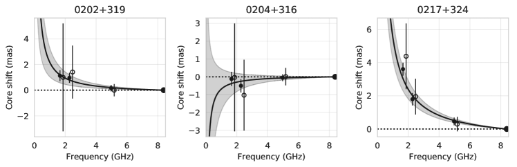
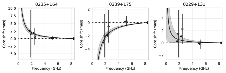
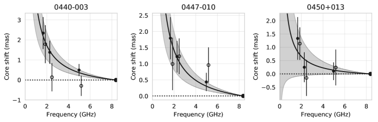
Figure 4: Frequency dependence of the core shifts relative to the X band measured for closely spaced triplets of sources. Filled circles show the results obtained using models with the estimated jet directions and the hollow circles the results obtained without applying these models. The projection of the core-shift vector onto the jet direction is shown. The curve and shaded region correspond to the dependence $\Delta r_{\textrm{core}}=a+b/\nu$, constructed using the filled circles and the 68$\%$ confidence interval about this fit. The results were obtained via our relative astrometry.

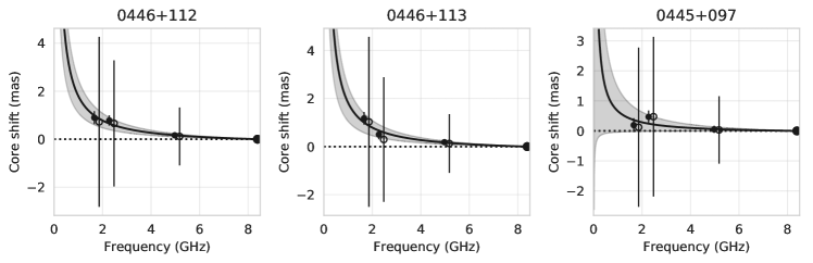
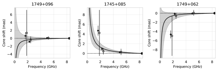
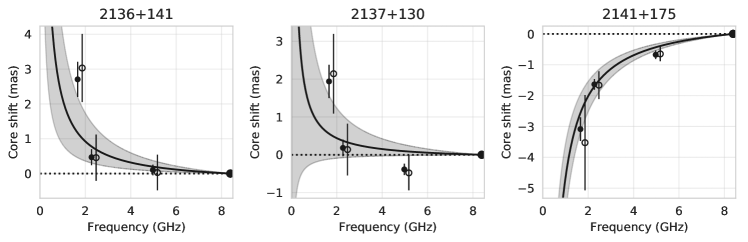
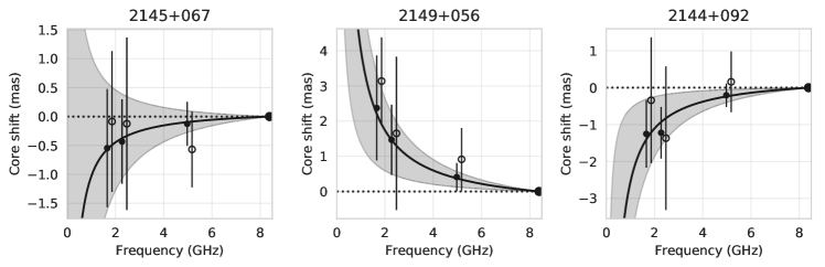
Figure 4: Continued

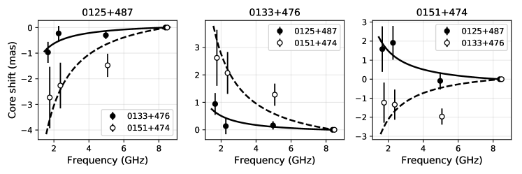
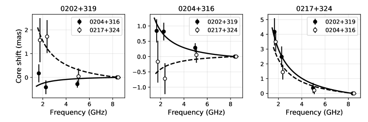
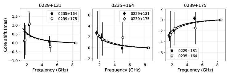
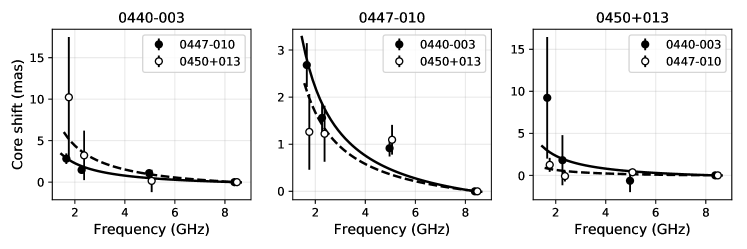
Figure 5: Frequency dependence of the core shift relative to the X band measured by expanding the relative shift vector into components along the jet directions of closely spaced sources considered in pairs. The solid and dotted curves show the dependences $\Delta r_{\textrm{core}}=a+b/\nu$ fitted using the filled and hollow points, respectively. The results were obtained via our relative astrometry.

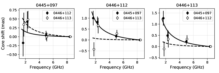
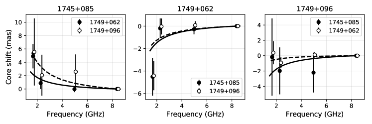
Figure 5: Continued

Table 1: Frequency-dependent core shifts relative to X-band (8.4 GHz), measured using the astrometric method (see Section 3.1). The values of the coefficient $b$ in the relation $r_{\mathrm{core}}(\nu)=b/\nu$ are also presented.

Source	Core shift (mas)			$b$ (mas GHz)
	X $\rightarrow$ L	X $\rightarrow$ S	X $\rightarrow$ C
0133+476	$1.25\pm 0.5$	$0.69\pm 0.4$	$0.18\pm 0.3$	$2.34\pm 1.3$
0125+487	$-1.39\pm 0.5$	$-0.98\pm 0.4$	$-0.39\pm 0.4$	$-2.92\pm 1.3$
0151+474	$0.16\pm 0.5$	$0.12\pm 0.4$	$-0.56\pm 0.5$	$0.28\pm 1.3$
0202+319	$1.12\pm 0.4$	$0.96\pm 0.4$	$0.15\pm 0.2$	$2.45\pm 1.3$
0204+316	$-0.12\pm 0.4$	$-0.50\pm 0.4$	$-0.05\pm 0.2$	$-0.78\pm 1.3$
0217+324	$3.60\pm 0.4$	$1.79\pm 0.4$	$0.46\pm 0.2$	$6.26\pm 1.5$
0235+164	$2.54\pm 0.3$	$1.81\pm 0.4$	$0.17\pm 0.3$	$5.13\pm 1.2$
0239+175	$-2.97\pm 0.3$	$-1.84\pm 0.4$	$0.13\pm 0.3$	$-5.67\pm 1.3$
0229+131	$0.26\pm 0.4$	$1.09\pm 0.3$	$-0.11\pm 0.2$	$1.32\pm 1.5$
0440$-$003	$2.34\pm 0.8$	$1.38\pm 0.6$	$0.50\pm 0.4$	$4.51\pm 1.8$
0447$-$010	$1.79\pm 0.6$	$1.22\pm 0.5$	$0.43\pm 0.4$	$3.71\pm 1.6$
0450+013	$1.33\pm 0.8$	$0.25\pm 0.6$	$0.10\pm 0.3$	$1.73\pm 1.9$
0446+112	$0.90\pm 0.3$	$0.78\pm 0.2$	$0.16\pm 0.1$	$2.04\pm 0.8$
0446+113	$1.17\pm 0.2$	$0.50\pm 0.2$	$0.18\pm 0.1$	$2.07\pm 0.8$
0445+097	$0.19\pm 0.2$	$0.47\pm 0.2$	$0.05\pm 0.1$	$0.75\pm 0.8$
1749+096	$0.63\pm 1.0$	$-0.86\pm 0.3$	$0.08\pm 0.2$	$-1.07\pm 2.2$
1745+085	$4.71\pm 1.0$	$0.94\pm 0.3$	$0.24\pm 0.2$	$3.41\pm 1.9$
1749+062	$-4.65\pm 0.8$	$-0.16\pm 0.3$	$-0.05\pm 0.2$	$-1.44\pm 2.1$
2136+141	$2.71\pm 0.5$	$0.47\pm 0.2$	$0.10\pm 0.2$	$2.42\pm 1.8$
2137+130	$1.94\pm 0.4$	$0.18\pm 0.2$	$-0.39\pm 0.2$	$1.15\pm 1.7$
2141+175	$-3.09\pm 0.4$	$-1.64\pm 0.2$	$-0.68\pm 0.2$	$-5.29\pm 1.3$
2145+067	$-0.55\pm 1.1$	$-0.43\pm 0.8$	$-0.13\pm 0.4$	$-1.17\pm 2.3$
2149+056	$2.37\pm 1.3$	$1.47\pm 0.9$	$0.41\pm 0.4$	$4.56\pm 2.7$
2144+092	$-1.25\pm 1.0$	$-1.22\pm 0.7$	$-0.21\pm 0.3$	$-2.90\pm 2.1$

4 RESULTS AND DISCUSSION

4.1 Relative Astrometric Measurements

The results of our measurements of the frequency-dependent VLBI core shift obtained via relative astrometry for simultaneous observations of triplets of sources are presented in Table 1. The shifts in mas for the L (1.7 GHz), S (2.3 GHz), and C (5.0 GHz) bands relative to the (highest-frequency) X-band (8.4 GHz) are given for each source. Positive values correspond to shifts of the core downward along the jet with decreasing frequency, as is predicted theoretically. Figure 4 shows the core shifts as a function of frequency.

We expect theoretically that $r_{\textrm{core}}\propto\nu^{-1/k_{\textrm{r}}}$ Lobanov (1998), but the measurement uncertainties hindered our ability to estimate $k_{\textrm{r}}$. Therefore, we fitted the dependence $\Delta r_{\textrm{core}}=a+b/\nu$, assuming $k_{\textrm{r}}=1$, which is a good approximation for most sources Sokolovsky et al. (2011). For many sources in our sample the estimated uncertainties exceed the measured shifts. At the same time, the measured core shifts for 0133+476, 0202+319, 0217+324, 0235+164, 0440$-$003, 0446+112, 0446+113, 0447$-$010, and 2149+056 are in good agreement with the dependence $\propto\nu^{-1}$. The median core shifts for these sources were 1.79, 1.22, and 0.18 mas for L, S, and C bands, respectively, relative to X band.

Note the reverse core shifts indicated for a number of the sources. We do not yet have a clear explanation for this result. It is important to understand whether this is an intrinsic astrophysical effect or the result of factors we have not taken into account in the method used. We did not detect this effect earlier in our core-shift measurements for large numbers of sources using the self-referencing method Pushkarev et al. (2012); Plavin et al. (2018). It is possible that only astrometric measurements are sensitive to this effect, or that some systematics are in the data, which we have not taken into account. Further studies of this effect require new, better quality, sensitive core-shift measurements. Such studies should be carried out, first and foremost, for sources that have manifest reverse core shifts in our observations.

For comparison, we measured the core shifts using the relative astrometry method when the relative shift vectors $\mathbf{CS}_{\textrm{rel}}$ for pairs of sources were spread around the jet directions. The results are shown in Fig. 5. Since we observed triplets of closely spaced sources related by a single phase solution, we obtained two measurements for each object. These plots show that the measurements for a given source and their uncertainties can depend strongly on which source in the pair is used to make the measurements. This is related to the different distances between the sources and the angles between their jet directions. Nevertheless, in most cases, the results of these pairwise core-shift measurements agree with the results obtained for the triplets as a whole.

Table 2: Core shifts measured by alignment pairs of images at different frequencies (Section 4.2)

Source	Frequency 1	Frequency 2	Core shift (mas)
			Right Ascension	Declination	Along jet	Perpendicular to jet
0133+476	C	L	$-0.46$	$0.90$	$1.01$	$-0.02$
0133+476	C	S	$-0.22$	$0.92$	$0.92$	$-0.24$
0133+476	X	C	$-0.05$	$0.29$	$0.28$	$-0.09$
0151+474	C	L	$-0.04$	$-0.33$	$0.33$	$-0.04$
0151+474	X	L	$-0.10$	$-0.68$	$0.68$	$-0.09$
0151+474	X	S	$-0.02$	$-0.60$	$0.60$	$-0.01$
0202+319	C	L	$0.11$	$0.48$	$0.49$	$-0.05$
0202+319	C	S	$0.11$	$0.31$	$0.32$	$-0.08$
0202+319	X	S	$-0.02$	$0.58$	$0.58$	$0.09$
0202+319	X	C	$-0.03$	$0.07$	$0.07$	$0.04$
0204+316	C	S	$0.58$	$-0.50$	$0.74$	$0.23$
0204+316	X	L	$0.78$	$-0.99$	$1.25$	$0.14$
0204+316	X	S	$0.43$	$-1.10$	$1.16$	$-0.22$
0204+316	X	C	$0.19$	$-0.34$	$0.39$	$-0.02$
0229+131	C	L	$0.68$	$0.36$	$0.77$	$-0.00$
0229+131	C	S	$0.42$	$0.26$	$0.49$	$0.03$
0239+175	C	S	$-0.28$	$0.59$	$0.65$	$0.01$
0445+097	C	L	$-1.17$	$-0.21$	$1.01$	$-0.63$
0445+097	C	S	$-0.64$	$-0.42$	$0.76$	$-0.11$
0446+113	C	L	$0.72$	$-0.56$	$0.88$	$0.23$
0446+113	C	S	$0.14$	$-0.01$	$0.10$	$0.10$
0447$-$010	C	L	$0.89$	$-1.15$	$1.42$	$0.33$
0447$-$010	C	S	$0.65$	$-0.81$	$1.01$	$0.26$
0450+013	C	S	$-0.77$	$-0.53$	$0.89$	$-0.29$
1745+085	C	S	$-0.25$	$-0.33$	$0.40$	$-0.07$
1745+085	X	S	$-0.32$	$-0.51$	$0.60$	$-0.06$
1745+085	X	C	$-0.32$	$-0.13$	$0.26$	$-0.23$
1749+062	X	C	$0.20$	$-0.58$	$0.61$	$0.05$
2144+092	S	L	$0.21$	$0.07$	$0.22$	$0.03$
2144+092	C	L	$0.71$	$0.23$	$0.74$	$0.10$
2144+092	C	S	$0.65$	$0.06$	$0.65$	$-0.06$
2144+092	X	L	$1.06$	$0.25$	$1.09$	$0.06$
2144+092	X	S	$0.80$	$0.08$	$0.81$	$-0.06$
2144+092	X	C	$0.25$	$-0.03$	$0.25$	$-0.07$
2145+067	C	L	$0.45$	$-0.51$	$0.67$	$-0.13$
2145+067	C	S	$0.23$	$-0.27$	$0.35$	$-0.07$

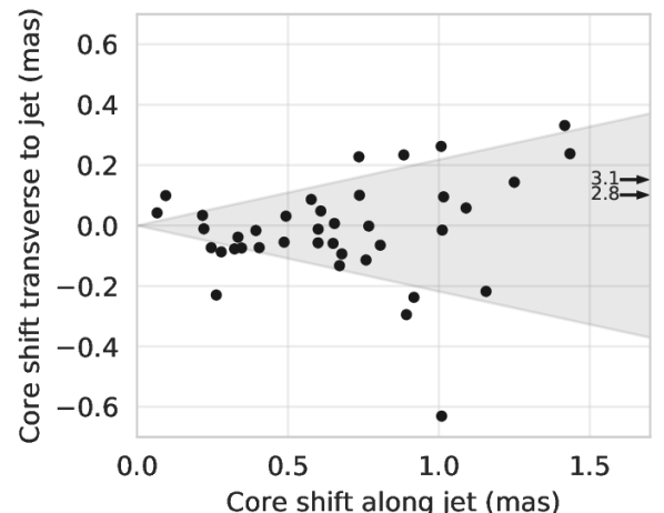
Figure 6: Measured core shifts relative to the jet directions. The arrows show two measurements that appreciably exceed the others; the numbers next to these arrows denote their positions along the horizontal axis. 68$\%$ of the shifts lie within $12^{\circ}$ of the horizontal direction, shaded in the figure. The typical estimated uncertainties are 0.3 mas.

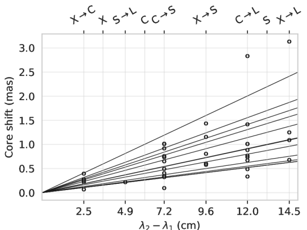
Figure 7: Dependence of the core shift measured via independent alignment of image pairs of a given source at different bands on the difference between corresponding wavelengths. Assuming $r_{\textrm{core}}\propto\nu^{-1}\propto\lambda$, the dependence for each source is a straight line. Only sources whose shifts were measured for more than one pair of frequencies are shown. The individual measurements and the best-fit linear approximation for each source are depicted. No uncertainties are shown; typical uncertainties are 0.3 mas. The symbols X, C, and S denote the values $\lambda_{2}-\lambda_{1}$, corresponding to the shifts from the position at the indicated band to the jet apex (i.e., $\lambda_{1}=0$). The lines correspond to the sources (from the bottom up): 0202+319, 0151+474, 0446+113, 2145+067, 0229+131, 2144+092, 1745+085, 0445+097, 0133+476, 0204+316, and 0447$-$010.

4.2 Core-shift Measurements by Images Alignment at Different Frequencies

The core shifts for sources with fairly extended structures can also be measured by aligning images of the source obtained at pairs of frequencies, as is described in Plavin et al. (2018). The reconstructed images were convolved with identical beams corresponding to the mean beam size for all the frequencies. The core position was determined via modeling of the source structure as a set of circular Gaussian components (see Section 2.5). It was possible to determine the core shifts for one or more pairs of frequencies for 15 sources in this way (41 frequency pairs in all). Figure 6 shows that these measured core shifts are in good agreement with the assumption that they should lie along the jet.

Since the core shifts for 12 sources were measured for more than one frequency pair, this makes it possible to study the frequency dependence of these shifts. We fitted a model assuming a dependence of the form $r_{\textrm{core}}\propto\nu^{-1/k_{\textrm{r}}}$ to the core-shift measurements obtained. This fitting placed essentially no limits on the value of $k_{r}$, which ranged from $0.6$ to infinity. Therefore, we assumed $k_{\textrm{r}}=1$ for our subsequent analysis, in agreement with the earlier results of Sokolovsky et al. (2011): $r_{\textrm{core}}\propto\nu^{-1}\propto\lambda$ and $\Delta r_{\textrm{core}}\propto\lambda_{2}-\lambda_{1}$. Figure 7 shows the dependence of the core shift on the difference between the wavelengths used to determine it.

The typical core shifts measured between X and S bands (8 and 2 GHz) in the current study, 0.65 mas, is in good agreement with the results of Kovalev et al. (2008); Sokolovsky et al. (2011); Plavin et al. (2018), where the median shift $X\to S$ is estimated to be 0.44, 0.71, and 0.53 mas, respectively.

Note that we were able to measure the shift between S and L bands (2.3 and 1.7 GHz) for only one source. This came about because these frequencies are fairly close, and the resolution obtained at these frequencies is a factor of three to four lower than the resolution obtained at X and C band. Two measurements appreciably exceeding the typical core-shift values were obtained for 0217+324: $2.8$ and $3.1$ mas for the frequency pairs $C\to L$ and $X\to L$, respectively, shown by the arrows in Fig. 6. A comparison of the L-band image of this source with the other L-band images indicates that there were no methodological errors in the measurements. This suggests that we are seeing some more distant region of the jet at L band that is brighter than the L-band core. This requires a separate study based on images with higher sensitivity.

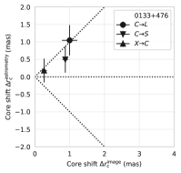
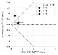
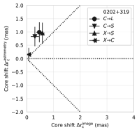
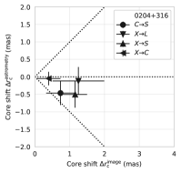
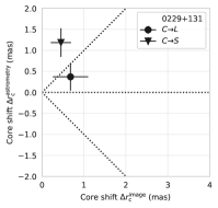
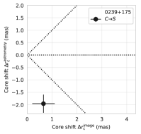
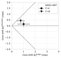
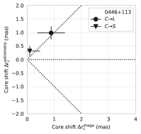
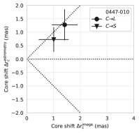
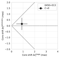
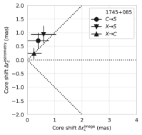
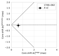
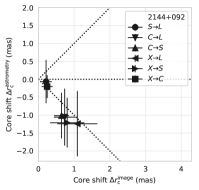
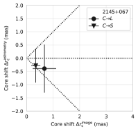
Figure 8: Comparison of the core shifts measured using two methods: images alignment at different frequencies, $\Delta r_{\textrm{c}}^{\textrm{image}}$ (Section 4.2) and applying the astrometric method $\Delta r_{\textrm{c}}^{\textrm{astrometry}}$ (Section 3.1, Fig. 4). The dotted lines show $\Delta r_{\textrm{c}}^{\textrm{astrometry}}=\pm\Delta r_{\textrm{c}}^{\textrm{image}}$ and $\Delta r_{\textrm{c}}^{\textrm{astrometry}}=0$.

Figure 8 presents a comparison of the results obtained using the various methods considered. For three of five sources with good $uv$-coverage, that is, with high declinations (the first five objects in this figure, which have declinations ${>}30^{\circ}$), the results for the two methods are fairly similar and show the same frequency dependence. A variety of behavior is seen in the remaining cases, from good agreement (e.g., 1745+085) to completely opposite results, i.e., with the shifts directed in opposite directions (e.g., 2144+092).

Table 3: Physical parameters of the sources (see Section 4.3). $r_{X}$ is the distance from the jet apex to the visible core in the X band (8 GHz) projected onto the sky and $B_{1}$ is the magnetic field 1 pc from the jet apex

Source	$r_{X}$		$B_{1}$, G
	mas	pc
0133+476	0.39	3.03	1.49
0151+474	0.16	1.34	0.72
0202+319	0.15	1.33	0.85
0204+316	0.42	3.55	2.07
0217+324	0.59
0229+131	0.24	2.02	1.53
0445+097	0.34	2.88	2.21
0446+113	0.15	1.33	0.82
0447$-$010	0.46	2.81	1.04
1745+085	0.27
2144+092	0.27	2.26	1.26
2145+067	0.19	1.51	0.80

4.3 Geometry and Physical Parameters

All of our conclusions about the physical structure of the jet presented in this section are based on our core-shift measurements obtained by alignment of images at different frequencies (Section 4.2). The astrometric method (Section 3.1) sometimes yields results that are not in agreement with our basic assumption that core shift is due to synchrotron self-absorption at the bases of the jets. Additional measurements and verification are required to more fully understand those measurements.

Assuming that, on average, the position of the core as a function of the wavelength is $r_{\textrm{core}}\propto\lambda$, we can estimate the distance from the intrinsic base (apex) of the jet (corresponding to $\lambda_{1}=0$ in the formulas above) to the core observed at a given frequency. The core positions at X, C, and S bands are given in Fig. 7. The typical distance from the jet apex to the 8 GHz core is 0.27 mas, or 2.1 pc projected onto the sky. The intrinsic distance from the jet apex to the 8 GHz core is ${\sim}20$ pc for a jet with a typical angle to the line of sight of $\theta\sim 6^{\circ}$ Hovatta et al. (2009).

We can use the measured core shifts to estimate the magnetic-field strength near the base of the jet. Assuming equipartition between the energies of the magnetic field and particles, and adopting a spectral index for the jet $\alpha={-}0.5$, which is taken to be observed at close to the critical angle (for which the apparent component speed $\beta_{\textrm{app}}$ is maximum), the magnetic field in Gauss at a distance of 1 pc from the intrinsic jet base can be estimated as follows Pushkarev et al. (2012):

$$B_{1}\approx 0.042\Omega_{\textrm{rv}}^{3/4}(1+z)^{1/2}(1+\beta_{\textrm{app}}^{2})^{1/8}\,,$$ (7)

where $\beta_{\textrm{app}}$ is the apparent speed of the jet and $\Omega_{\textrm{rv}}$ a parameter corresponding to the core shift measured in pc$\cdot$GHz. Since the dependence of $B_{1}$ on $\beta_{\textrm{app}}$ is weak ($B_{1}$ increases by only a factor of 1.8 as $\beta_{\textrm{app}}$ increases from 0 to 10), We used the fixed factor $(1+\beta_{\textrm{app}}^{2})^{1/8}=1.5$, which corresponds to $\beta_{\textrm{app}}=5$. The mean magnetic field 1 pc from the intrinsic jet apex is then $B_{\text{1,mean}}=1.2$ G; values for individual sources are presented in Table 3.

5 CONCLUSION

We have developed two approaches to measuring the frequency-dependent core shifts of each source in a group of closely spaced quasars, which are related by a single phase solution derived from VLBI relative astrometry. In one approach, the difference in the core shifts for two sources is written in terms of contributions in the directions of the relativistic jets of each, assuming that the shifts occur along these directions. In the other approach, we use measurements of an arbitrary number of closely spaced sources to estimate the core shifts taking into account a priori information about the jet directions, for either all or only some of the sources.

We organized pilot observations of eight triplets of compact extragalactic radio sources on the EVN to test these methods. Three telescopes of the Russian Kvazar–KVO array took part in these observations. Their participation improved the resulting measurement accuracy and the sensitivity and quality of the reconstructed images. Unfortunately, the failure of the Hartebeeshoek telescope in South Africa led to a loss of long baselines in the North–South direction, which appreciably lowered the accuracy of the measurements.

We have estimated the frequency-dependent core shifts for the 24 objects included in this study. The measured core shifts for nine of these are significant. For these sources, the median VLBI core shifts at 1.7, 2.3, and 5.0 GHz relative to our highest frequency, 8.4 GHz, were 1.79, 1.22, and 0.18 mas, respectively. We were able to independently measure the core shifts of a number of sources via self-referencing using extended, optically thin regions in the source. For these, we have also estimated the distance from the 8.4 GHz VLBI core to the intrinsic base of the relativistic jet and the magnetic-field strength 1 pc from this base. The typical values of these quantities for these sources were 2 pc projected onto the sky and 1.2 G.

We conclude that the relative-astrometry method can be used to measure frequency-dependent VLBI core shifts for very compact sources for which other methods are not suitable. This is especially important for objects defining the highest-accuracy inertial reference frame available — the International Celestial Reference Frame (ICRF) — which is based on VLBI measurements. Achieving the required accuracy and reliability of these measurements requires VLBI observations with good $uv$-coverage, high sensitivity, and high angular resolution.

Table 4: Map parameters

Source	Frequency (GHz)	$I_{\text{peak}}$ (mJy/beam)	rms (mJy/beam)	$S_{\text{tot}}$ (mJy)	$\theta_{\text{maj}}$ (mas)	$\theta_{\text{min}}$ (mas)	$PA_{\text{beam}}$ (deg)
0125+487	1.659	$192$	0.13	$262$	$10.25$	$4.84$	$17.8$
	2.273	$233$	0.67	$361$	$5.13$	$2.54$	$16.7$
	4.975	$314$	0.12	$370$	$3.02$	$1.51$	$16.3$
	8.385	$394$	0.17	$455$	$1.76$	$0.87$	$16.0$
0133+476	1.659	$1277$	0.31	$1768$	$9.11$	$4.04$	$17.8$
	2.273	$1608$	0.67	$2489$	$5.34$	$2.59$	$20.1$
	4.975	$2317$	0.31	$2959$	$2.70$	$1.25$	$16.4$
	8.385	$3039$	0.43	$3701$	$1.55$	$0.70$	$22.6$
0151+474	1.659	$234$	0.16	$308$	$10.86$	$4.98$	$20.3$
	2.273	$380$	0.68	$455$	$5.28$	$2.64$	$22.0$
	4.975	$550$	0.11	$603$	$2.94$	$1.48$	$18.6$
	8.385	$638$	0.22	$702$	$1.71$	$0.83$	$24.5$
0202+319	1.659	$729$	0.27	$988$	$14.21$	$4.21$	$10.8$
	2.273	$1026$	0.37	$1331$	$7.33$	$2.45$	$9.5$
	4.975	$1820$	0.25	$2001$	$3.75$	$1.30$	$6.7$
	8.385	$2861$	0.47	$3078$	$2.29$	$0.74$	$9.6$
0204+316	1.659	$237$	0.17	$608$	$15.05$	$4.42$	$11.3$
	2.273	$271$	0.50	$662$	$7.42$	$2.44$	$10.9$
	4.975	$194$	0.12	$396$	$4.27$	$1.45$	$7.9$
	8.385	$164$	0.20	$273$	$2.64$	$0.85$	$13.3$
0217+324	1.659	$457$	0.18	$825$	$14.47$	$4.35$	$12.1$
	2.273	$359$	0.59	$765$	$7.14$	$2.47$	$11.6$
	4.975	$160$	0.14	$428$	$4.24$	$1.42$	$8.8$
	8.385	$131$	0.14	$320$	$2.51$	$0.82$	$14.4$
0229+131	1.659	$1117$	0.50	$1508$	$20.10$	$4.14$	$9.3$
	2.273	$1693$	0.85	$1996$	$9.39$	$2.54$	$8.6$
	4.975	$1679$	0.29	$2029$	$4.87$	$1.23$	$6.3$
	8.385	$1398$	0.39	$1954$	$3.30$	$0.69$	$10.0$
0235+164	1.659	$2038$	1.16	$2088$	$18.05$	$3.98$	$10.4$
	2.273	$2906$	0.78	$3037$	$8.97$	$2.54$	$10.6$
	4.975	$4751$	0.48	$4930$	$4.27$	$1.20$	$7.0$
	8.385	$6552$	0.58	$6849$	$2.75$	$0.63$	$10.6$
0239+175	1.659	$154$	0.06	$180$	$21.30$	$4.71$	$10.3$
	2.273	$183$	0.67	$251$	$9.07$	$2.51$	$11.2$
	4.975	$187$	0.10	$229$	$5.52$	$1.43$	$7.3$
	8.385	$257$	0.16	$283$	$3.50$	$0.82$	$10.8$
0440$-$003	1.659	$2551$	1.27	$2655$	$25.53$	$4.21$	$6.1$
	2.273	$3023$	0.92	$3343$	$11.80$	$2.43$	$7.3$
	4.975	$1676$	0.36	$2190$	$6.24$	$1.17$	$4.4$
	8.385	$1095$	0.45	$2017$	$4.09$	$0.71$	$7.2$
0445+097	1.659	$186$	0.63	$366$	$30.15$	$4.73$	$6.1$
	2.273	$207$	0.62	$324$	$10.63$	$2.39$	$7.0$
	4.975	$260$	0.31	$324$	$6.23$	$1.49$	$4.1$
	8.385	$399$	0.24	$469$	$3.98$	$0.89$	$7.6$
0446+112	1.659	$726$	0.62	$1174$	$23.51$	$4.04$	$5.8$
	2.273	$861$	0.49	$1348$	$10.33$	$2.40$	$7.3$
	4.975	$735$	0.17	$1000$	$5.75$	$1.26$	$4.3$
	8.385	$907$	0.22	$1232$	$3.79$	$0.78$	$7.8$
0446+113	1.659	$125$	0.06	$267$	$24.27$	$4.27$	$5.9$
	2.273	$151$	0.54	$299$	$10.53$	$2.39$	$6.9$
	4.975	$313$	0.15	$414$	$5.91$	$1.45$	$3.9$
	8.385	$309$	0.24	$356$	$3.98$	$0.86$	$7.8$
0447$-$010	1.659	$146$	0.09	$180$	$31.45$	$4.77$	$6.2$
	2.273	$162$	0.60	$218$	$11.94$	$2.38$	$7.5$
	4.975	$115$	0.09	$159$	$7.20$	$1.50$	$4.5$
	8.385	$144$	0.17	$178$	$4.47$	$0.89$	$6.7$
0450+013	1.659	$62$	0.03	$90$	$29.94$	$4.82$	$6.3$
	2.273	$123$	0.62	$156$	$11.93$	$2.46$	$7.2$
	4.975	$143$	0.09	$161$	$7.14$	$1.52$	$4.5$
	8.385	$174$	0.18	$197$	$4.58$	$0.89$	$7.2$
1745+085	1.659	$82$	0.06	$246$	$28.69$	$5.80$	$2.3$
	2.273	$75$	0.57	$300$	$10.59$	$2.89$	$2.2$
	4.975	$96$	0.12	$211$	$6.94$	$1.97$	$2.2$
	8.385	$127$	0.12	$209$	$4.18$	$1.04$	$4.6$
1749+062	1.659	$377$	0.37	$460$	$28.07$	$5.61$	$3.4$
	2.273	$386$	0.52	$588$	$10.32$	$3.10$	$2.1$
	4.975	$289$	0.21	$395$	$6.99$	$1.86$	$3.5$
	8.385	$264$	0.17	$341$	$4.23$	$1.07$	$5.1$
1749+096	1.659	$996$	0.56	$1127$	$24.01$	$5.43$	$2.5$
	2.273	$1928$	0.52	$2123$	$10.20$	$2.97$	$1.3$
	4.975	$3346$	0.38	$3532$	$5.60$	$1.52$	$1.4$
	8.385	$5736$	1.22	$5941$	$3.18$	$0.93$	$2.4$
2136+141	1.659	$1632$	0.56	$1767$	$19.37$	$4.34$	$8.8$
	2.273	$2134$	0.70	$2536$	$9.13$	$2.60$	$7.2$
	4.975	$2418$	0.40	$3095$	$4.82$	$1.19$	$5.8$
	8.385	$2255$	0.55	$3580$	$3.09$	$0.67$	$9.6$
2137+130	1.659	$151$	0.05	$155$	$23.13$	$5.16$	$8.9$
	2.273	$215$	0.64	$241$	$9.33$	$2.57$	$7.4$
	4.975	$155$	0.11	$175$	$5.81$	$1.63$	$5.6$
	8.385	$151$	0.18	$171$	$3.59$	$0.92$	$9.0$
2141+175	1.659	$344$	0.16	$449$	$20.04$	$4.85$	$10.8$
	2.273	$357$	0.53	$423$	$8.75$	$2.59$	$7.7$
	4.975	$505$	0.15	$564$	$4.93$	$1.53$	$6.3$
	8.385	$608$	0.25	$686$	$3.18$	$0.85$	$9.2$
2144+092	1.659	$482$	0.16	$630$	$23.77$	$4.42$	$8.5$
	2.273	$551$	0.61	$740$	$10.09$	$2.50$	$6.6$
	4.975	$641$	0.14	$764$	$5.83$	$1.40$	$5.5$
	8.385	$785$	0.28	$918$	$3.72$	$0.88$	$8.3$
2145+067	1.659	$2146$	0.38	$3705$	$21.38$	$3.70$	$8.6$
	2.273	$3519$	1.65	$4962$	$10.30$	$2.41$	$7.1$
	4.975	$4108$	0.51	$6175$	$5.43$	$1.01$	$6.2$
	8.385	$4101$	1.34	$6847$	$3.42$	$0.62$	$8.8$
2149+056	1.659	$695$	0.23	$900$	$24.97$	$4.47$	$7.8$
	2.273	$926$	0.82	$1240$	$10.42$	$2.46$	$6.5$
	4.975	$724$	0.19	$907$	$6.22$	$1.35$	$5.7$
	8.385	$552$	0.31	$702$	$4.03$	$0.87$	$8.8$

Figure 9: Continued.

Figure 9: Continued.

Figure 9: Continued.

Figure 9: Continued.

References

- Blandford and Königl (1979) R. D. Blandford and A. Königl, ApJ 232, 34 (1979).
- Königl (1981) A. Königl, ApJ 243, 700 (1981).
- Lobanov (1998) A. P. Lobanov, A&A 330, 79 (1998).
- Kovalev et al. (2008) Y. Y. Kovalev, A. P. Lobanov, A. B. Pushkarev, and J. A. Zensus, A&A 483, 759 (2008).
- Hovatta et al. (2012) T. Hovatta, M. L. Lister, M. F. Aller, H. D. Aller, D. C. Homan, Y. Y. Kovalev, A. B. Pushkarev, and T. Savolainen, AJ 144, 105 (2012).
- Kravchenko et al. (2016) E. V. Kravchenko, Y. Y. Kovalev, T. Hovatta, and V. Ramakrishnan, MNRAS 462, 2747 (2016).
- Kravchenko et al. (2017) E. V. Kravchenko, Y. Y. Kovalev, and K. V. Sokolovsky, MNRAS 467, 83 (2017).
- Ma et al. (1998) C. Ma, E. F. Arias, T. M. Eubanks, A. L. Fey, A.-M. Gontier, C. S. Jacobs, O. J. Sovers, B. A. Archinal, and P. Charlot, AJ 116, 516 (1998).
- Petrov et al. (2009) L. Petrov, D. Gordon, J. Gipson, D. MacMillan, C. Ma, E. Fomalont, R. C. Walker, and C. Carabajal, Journal of Geodesy 83, 859 (2009).
- Petrov and Kovalev (2017a) L. Petrov and Y. Y. Kovalev, MNRAS 467, L71 (2017a).
- Kovalev et al. (2017) Y. Y. Kovalev, L. Petrov, and A. V. Plavin, A&A 598, L1 (2017).
- Petrov and Kovalev (2017b) L. Petrov and Y. Y. Kovalev, MNRAS 471, 3775 (2017b).
- Greisen (2003) E. W. Greisen, Information Handling in Astronomy - Historical Vistas 285, 109 (2003).
- Shepherd (1997) M. C. Shepherd, in Astronomical Data Analysis Software and Systems VI, Astronomical Society of the Pacific Conference Series, Vol. 125, edited by G. Hunt and H. Payne (1997) p. 77.
- Pushkarev et al. (2012) A. B. Pushkarev, T. Hovatta, Y. Y. Kovalev, M. L. Lister, A. P. Lobanov, T. Savolainen, and J. A. Zensus, A&A 545, A113 (2012).
- Salvatier et al. (2016) J. Salvatier, T. V. Wiecki, and C. Fonnesbeck, PeerJ Computer Science 2, e55 (2016).
- Kutkin et al. (2018) A. M. Kutkin, I. N. Pashchenko, M. M. Lisakov, P. A. Voytsik, K. V. Sokolovsky, Y. Y. Kovalev, A. P. Lobanov, A. V. Ipatov, M. F. Aller, H. D. Aller, A. Lahteenmaki, M. Tornikoski, and L. I. Gurvits, MNRAS 475, 4994 (2018).
- Lister et al. (2016) M. L. Lister, M. F. Aller, H. D. Aller, D. C. Homan, K. I. Kellermann, Y. Y. Kovalev, A. B. Pushkarev, J. L. Richards, E. Ros, and T. Savolainen, AJ 152, 12 (2016).
- Hovatta et al. (2014) T. Hovatta, M. F. Aller, H. D. Aller, E. Clausen-Brown, D. C. Homan, Y. Y. Kovalev, M. L. Lister, A. B. Pushkarev, and T. Savolainen, AJ 147, 143 (2014).
- Shapiro et al. (1979) I. I. Shapiro, J. J. Wittels, C. C. Counselman, III, D. S. Robertson, A. R. Whitney, H. F. Hinteregger, C. A. Knight, A. E. E. Rogers, T. A. Clark, L. K. Hutton, and A. E. Niell, AJ 84, 1459 (1979).
- Reid and Honma (2014) M. J. Reid and M. Honma, ARA&A 52, 339 (2014).
- Pradel et al. (2006) N. Pradel, P. Charlot, and J.-F. Lestrade, A&A 452, 1099 (2006).
- Sokolovsky et al. (2011) K. V. Sokolovsky, Y. Y. Kovalev, A. B. Pushkarev, and A. P. Lobanov, A&A 532, A38 (2011).
- Walker et al. (2000) R. C. Walker, V. Dhawan, J. D. Romney, K. I. Kellermann, and R. C. Vermeulen, ApJ 530, 233 (2000).
- O’Sullivan and Gabuzda (2009) S. P. O’Sullivan and D. C. Gabuzda, MNRAS 400, 26 (2009).
- Plavin et al. (2018) A. V. Plavin, Y. Y. Kovalev, A. B. Pushkarev, and A. P. Lobanov, MNRAS, submitted (2018).
- Marcaide and Shapiro (1984) J. M. Marcaide and I. I. Shapiro, ApJ 276, 56 (1984).
- Hovatta et al. (2009) T. Hovatta, E. Valtaoja, M. Tornikoski, and A. Lähteenmäki, A&A 494, 527 (2009).