Connection between asymptotic normalization coefficients and resonance widths of mirror states

Abstract

Asymptotic normalization coefficients (ANCs) are fundamental nuclear constants playing important role in nuclear reactions, nuclear structure and nuclear astrophysics. In this paper a connection between ANCs and resonance widths of the mirror states is established. Using Pinkston-Satchler equation the ratio for resonance widths and ANCs of mirror nuclei is obtained in terms of the Wronskians from the radial overlap functions and regular solutions of the two-body Schrödinger equation with the short-range interaction excluded. This ratio allows one to use microscopic overlap functions for mirror nuclei in the internal region, where they are the most accurate, to correctly predict the ratio of the resonance widths and ANCs for mirror nuclei, which determine the amplitudes of the tails of the overlap functions. If the microscopic overlap functions are not available one can express the Wronskians for the resonances and mirror bound states in terms of the corresponding mirror two-body potential-model wave functions. A further simplification of the Wronskians ratio leads to the equation for the ratio of the resonance widths and mirror ANCs, which is expressed in terms of the ratio of the two-body Coulomb scattering wave functions at the resonance energy and at the binding energy [N. K. Timofeyuk, R. C. Johnson, and A. M. Mukhamedzhanov, Phys. Rev. Lett. 91, 232501 (2003]. In this paper calculations of the ratios of resonance widths and mirror ANCs for different nuclei are presented. From this ratio one can determine the resonance width if the mirror ANC is known and vice versa. Comparison with available experimental ratios are done.

I Introduction

The asymptotic normalization coefficient (ANC) is a fundamental nuclear characteristics of bound states blokh77 ; blokhintsev84 playing an important role in nuclear reaction and structure physics. The ANCs determine the normalization of the peripheral part of transfer reaction amplitudes blokh77 ; blokhintsev84 and overall normalization of the peripheral radiative capture processes muktim90 ; muk90 ; muk2001 ; muk2011 . In the R-matrix approach the ANC determines the normalization of the external nonresonant radiative capture amplitude and the channel radiative reduced width amplitude muktr99 ; tang ; kroha2011 . In timofeyuk2003 ; muk2012 relationships between mirror proton and neutron ANCs were obtained.

However, the ANCs are important characteristics not only of the bound states but also resonances, see muktr99 . The width of a narrow resonance can be expressed in terms of the ANC of the Gamow wave function or of the $R$-matrix resonant outgoing wave. Because the ANC of a narrow resonance state is related to the resonance width of this state the relationship between the ANCs of mirror states timofeyuk2003 ; muk2012 can be extended to the relationship between the ANCs of the bound states and resonance widths of the mirror states. The first such attempt was done in timofeyuk2003 . In this paper the relationship between the ANCs and resonance widths is established based on the Pinkston-Satchler equation used in muk2012 for the ANCs of the mirror bound states. The obtained ratio of the resonance width and the ANC of the mirror bound state is expressed in terms of the ratio of the Wronskians containing the overlap functions of the mirror resonance and bound states in the internal region where these overlap functions can be calculated quite accurately using ab initio approach. If these overlap functions are not available, as an approximation they can be replaced by the mirror resonance and bound state wave functions calculated using the two-body potential model. Assuming that the mirror resonant and bound-state wave functions are identical in the nuclear interior one can replace the Wronskian ratio for the resonance width and the ANC of the mirror bound state by the equation derived in timofeyuk2003 , which does not require a knowledge of the internal resonant and bound-state wave functions.

Connection between the ANC and the resonance width of the mirror resonance state provides a powerful indirect method to obtain information, which is unavailable directly. If, for instance, the resonance width is unknown it can be determined through the known ANC of the mirror state and vice versa. For example, near the edge of the stability valley neutron binding energies become so small, that the mirror proton states are resonances. Using the relationship between the mirror resonance width and the ANC the resonance width can be determined. Also loosely bound states $\alpha+A$ become resonances in the mirror nucleus $\alpha+B$, where charge $Z_{B}e>Z_{A}e$. Using the method developed here one can find one of the missing quantities, the resonance width of the narrow resonance state or the mirror ANC. In what follows the system of units in which $\hbar=c=1$ is used throughout the paper.

I.1 ANC in the scattering theory and Schrödinger formalism

The ANC enters the theory in two ways blokh77 . In the scattering theory the residue at the poles of the elastic scattering $S$ matrix corresponding to bound states can be expressed in terms of the ANC:

$$S_{l_{B}\,j_{B};l_{B}\,j_{B}}^{J_{B}}\xrightarrow{k_{aA}\to k_{aA}^{bs}}\,\frac{A_{l_{B}\,j_{B}}}{k-i\,\kappa_{aA}}$$ (1)

with the residue

$$A_{l_{B}\,j_{B}}^{J_{B}}=-i^{2\,l_{B}+1}\,e^{i\,\pi\,\eta_{aA}^{bs}}\,\big{(}C^{B}_{aA\,l_{B}\,j_{B}\,J_{B}}\big{)}^{2}.$$ (2)

Here, $\,C^{B}_{aA\,l_{B}\,j_{B}\,J_{B}}$ is the ANC for the virtual decay of the bound state $B(aA)$ in the channel with the relative orbital angular momentum $\,\,l_{B}$ of $a$ and $A$, the total angular momentum $\,\,j_{B}$ of $a$ and total angular momentum $\,\,J_{B}$ of the system $a+A$, $k_{aA}$ is the relative momentum of particles $a$ and $A$.

$$\eta_{aA}^{bs}=\frac{Z_{a}\,Z_{A}\,e^{2}\,\mu_{aA}}{\kappa_{aA}}$$ (3)

is the Coulomb parameter for the bound state $B=(a\,A)$, $\;\kappa_{aA}=\sqrt{2\,\mu_{aA}\,\varepsilon_{aA}}$ is the bound-state wave number, $\,\varepsilon_{aA}=m_{a}+m_{A}-m_{B}$ is the binding energy for the virtual decay $B\to a+A$, $Z_{i}\,e$ and $m_{i}$ is the charge and mass of particle $i$, and $\mu_{aA}$ is the reduced mass of $a$ and $A$. Note that the singling out the factor $e^{i\,\pi\,\eta_{aA}^{bs}}$ in the residue makes the ANC for bound states real.

Equations (1) and (2), which were proved for the bound states in kramers ; heisenberg ; meller ; hu ; zeldovich ; perelomov , can be extended for resonance states.

II Connection between ANC and resonance width

The proof of the connection between the residue in the resonance pole of the elastic scattering $S$ matrix and the ANC of the resonance state is not trivial. In this section is presented a general proof of the connection of the residue in the pole of the $S_{l_{B}}(k_{aA})$ matrix element with the ANC , which is valid both for the bound states and resonances. The potential is given by the sum of the short-range nuclear plus the long-range Coulomb potentials. Taking into account that the residue of the elastic scattering $S$ matrix in the resonance pole is expressed in terms of the resonance width, one can obtain a connection between the ANC and the resonance width.

Let me consider two spinless particles $a$ and $A$ with relative momentum $k_{aA}^{2}=2\,\mu_{aA}\,E_{aA}$, relative energy $E_{aA}$ and the reduced mass $\mu_{aA}$ in the partial wave $l_{B}$ at which the system $B=a+A$ has a resonance or a bound state. The radial wave function $\psi_{k_{aA}l_{B}}(r)=\frac{u_{k_{aA}l_{B}}(r)}{r}$ satisfies the Schrödinger equation in the partial wave $l_{B}$:

$$\frac{{\partial}^{2}u_{k_{aA}l_{B}}(r)}{{\partial{r}^{2}}}+\big{[}k_{aA}^{2}-2{\mu_{aA}}V(r)\,\,-\,\frac{{l_{B}(l_{B}+1)}}{{{r^{2}}}}\big{]}u_{k_{aA}l_{B}}(r)=0.$$ (4)

Here $V(r)=V^{N}(r)+V^{C}(r)$, $\,V^{N}(r)$ is the short-range nuclear potential and $V^{C}(r)$ is the long-range Coulomb one. For potentials satisfying the condition $\mathop{\lim}\limits_{r\to 0}r^{2}\,V(r)\to 0$

$$u_{k_{aA}l_{B}}(r)\sim r^{l_{B}+1},\qquad r\to 0.$$ (5)

Now one should take the derivative over $k_{aA}$ from the left-hand-side of Eq. (4), multiply the result by $u_{k_{aA}l_{B}}(r)$ and subtract from it Eq. (4) multiplied by $\partial{u_{k_{aA}l_{B}}}(r)/\partial k_{aA}$. Integrating the obtained expression from $r=0$ until $r=R$ and taking into account Eq. (5) one gets

$$\int\limits_{0}^{R}{dr\,u_{k_{aA}l_{B}}^{2}(r)=\,\frac{1}{{2k_{aA}}}\left[{\frac{{\partial{u_{k_{aA}l_{B}}}(R)}}{{\partial k_{aA}}}\frac{{\partial{u_{k_{aA}l_{B}}}(R)}}{{\partial R}}-{u_{k_{aA}l_{B}}}(R)\frac{{{\partial^{2}}{u_{k_{aA}l_{B}}}(R)}}{{\partial k_{aA}\,\partial R}}}\right]}.$$ (6)

Taking $R$ so large that $u_{k_{aA}l_{B}}(R)$ can be replaced by its leading asymptotic term one gets

$${u_{k_{aA}l_{B}}}(R)\approx{{\tilde{C}}_{l_{B}}}\left[{{e^{i\rho}}-{{(-1)}^{l}_{B}}S_{l_{B}}^{-1}(k_{aA}){e^{-i\rho}}}\right],$$ (7)

where $\rho=k_{aA}R-\eta_{aA}\,\ln\,2k_{aA}R,\,\,\,\,\,\,\,\eta_{aA}=({Z_{a}}{Z_{A}}/137){\mu_{aA}}/k_{aA}\,$ is the Coulomb parameter of the $a+A$ system.

$$S_{l_{B}}(k_{aA})=e^{2\,i\,[\delta_{l_{B}}^{C}(k_{aA})+\delta_{l_{B}}^{CN}(k_{aA})]}$$ (8)

is the elastic scattering $S$-matrix element, $\delta_{l_{B}}^{C}(k_{aA})$ and $\delta^{CN}_{l_{B}}(k_{aA})$ are the Coulomb and Coulomb-modified nuclear scattering phase shifts in the $l_{B}$-th partial wave. ${\tilde{C}}_{l_{B}}$ does not depend on $k_{aA}$ and can be determined from the normalization condition of the bound or resonance state wave functions.

Assume now that the elastic scattering $S_{l_{B}}(k_{aA})$-matrix element has a first order pole at $k_{aA}=k_{p}$ with the residue $A_{l_{B}}$ corresponding to the bound state $k_{p}=i\,\kappa_{aA}$ and to the resonance state $k_{p}=k_{aA(R)}=k_{aA\,(0)}-{\rm Im}k_{aA\,(R)},$ where $\;k_{aA\,(0)}={\rm Re}k_{aA\,(R)}$:

$$S_{l_{B}}(k_{aA})=\frac{A_{l_{B}}}{k_{aA}-k_{p}}+g_{l_{B}}(k_{AA}),$$ (9)

$g_{l_{B}}(k_{aA})$ is a regular function at $k_{aA}=k_{p}$.

Substituting Eqs (7) and (9) into the right-hand-side of Eq. (6) and performing the differentiation over $k_{aA}$ and $R$ and taking $k_{aA}=k_{p}$ one gets

$$\int\limits_{0}^{R}{\rm d}r\,u_{k_{p}l_{B}}^{2}(r)=i\,(-1)^{l_{B}+1}{\tilde{C}}_{l_{B}}^{2}/A_{l_{B}}-\frac{i}{2\,k_{p}}\,e^{2\,i\,\rho_{0}}.$$ (10)

On the left-hand-side under the integral sign we have the function $u_{k_{p}l_{B}}^{2}(r)$, which is regular at $r=0$ (see Eq. (5) and satisfies the radiation condition:

$$u_{k_{p}l_{B}}(r)\stackrel{{\scriptstyle r>R_{N}}}{{=}}C_{l_{B}}\,W_{-i\,\eta_{p},\,l_{B}+1/2}(-2\,i\,k_{p}\,r).$$ (11)

Here $R_{N}$ is the $a-A$ nuclear interaction radius. For the bound state $k_{p}=i\,\kappa_{aA}$ and

$$u_{i\,\kappa_{aA}l_{B}}(r)\stackrel{{\scriptstyle r>R_{N}}}{{=}}C_{l_{B}}\,W_{-\eta_{aA}^{bs},\,l_{B}+1/2}(2\,k_{p}\,r)\stackrel{{\scriptstyle r\to\infty}}{{\approx}}C_{l_{B}}e^{-\kappa_{aA}\,r-\eta_{aA}^{bs}\,\ln(2\,\kappa_{aA}\,r)}.$$ (12)

For the resonance state $k_{p}=k_{aA(R)}$ and $u_{k_{aA(R)}l_{B}}(r)$ is the resonance Gamow wave function with the resonance energy $E_{aA(R)}$:

$$u_{k_{aA(R)}l_{B}}(r)\stackrel{{\scriptstyle r>R_{N}}}{{=}}C_{l_{B}}\,W_{-i\,\eta_{aA}^{R},\,l_{B}+1/2}(-2\,i\,k_{aA(R)}\,r)\stackrel{{\scriptstyle r\to\infty}}{{\approx}}e^{-\pi\,\eta_{aA}^{R}/2}\,C_{l_{B}}e^{i\,k_{aA(R)}\,r-i\,\eta_{aA}^{R}\,\ln(2\,k_{aA(R)}\,r)}$$

$$={\tilde{C}}_{l_{B}}e^{i\,k_{aA(R)}\,r-i\,\eta_{aA}^{R}\,\ln(2\,k_{aA(R)}\,r)}.$$ (13)

Here, $\eta_{aA}^{R}=\,\frac{Z_{a}\,Z_{A}\,e^{2}\,\mu_{aA}}{k_{aA\,(R)}}$ the $a-A$ Coulomb parmeter of the resonance. For the resonance

$${\tilde{C}}_{l_{B}}=e^{-\pi\,\eta_{aA}^{R}/2}\,C_{l_{B}}.$$ (14)

Thus one can use two equivalent definitions of the ANC, which differ by a factor of $e^{-\pi\,\eta_{aA}^{R}/2}$ for the resonance state. Formally, one can use two definitions of the ANC for the bound states:

$${\tilde{C}}_{l_{B}}=e^{i\,\pi\,\eta_{aA}^{bs}/2}\,C_{l_{B}}.$$ (15)

However, the $C_{l_{B}}$, which is real for the bound states, is the standard definition of the ANC for the bound states and will be used in this paper for the bound states.

Also the following definitions are used:

$$E_{aA(R)}=k_{aA(R)}^{2}/(2\,\mu_{aA})=E_{aA(0)}-i\,\Gamma_{aA}/2,\qquad E_{aA(0)}=\big{[}k_{aA(0)}^{2}-({\rm Im}k_{aA(R)})^{2}\big{]}/(2\,\mu_{aA}),$$

$$\Gamma_{aA}=2\,k_{aA(0)}\,{\rm Im}k_{aA(R)}/\mu_{aA}.$$ (16)

For the bound states the asymptotic of the bound state wave is exponentially decaying and the bound-state wave function can be normalized. For the resonance state the Gamow wave function asymptotically oscillates and exponentially increasing. To normalize the Gamow wave function one can use Zeldovich regularization procedure zeldovich which is a particular case of the more general Abel regularization:

$$\lim\limits_{\beta\to+0}\,\int\limits_{0}^{\infty}\,{\rm d}re^{-\beta\,r^{2}}\,u_{k_{aA(R)}l_{B}}^{2}(r)=1.$$ (17)

For the bound state one can take under the integral sign $\beta=0$ and obtain the usual normalization procedure. For the resonance state one can take the limit $\beta\to 0$ only after performing the integration over $t$. Note that Zel’dovich normalization was introduced for exponentially decaying potentials. In Appendix A is shown that Zel’dovich regularization procedure works even for the Coulomb potentials.

For any finite $R\,$ one can rewrite Eq. (17) as

$$\int\limits_{0}^{R}\,{\rm d}r\,u_{k_{aA(R)}}^{2}(r)+\lim\limits_{\beta\to+0}\,\int\limits_{R}^{\infty}\,{\rm d}re^{-\beta\,r^{2}}\,u_{k_{aA(R)}l_{B}}^{2}(r)=1.$$ (18)

Assume that $R$ is so large that one can use the asymptotic expression (11) and Eq. (A.5) of Appendix. It leads to

$$\int\limits_{0}^{R}\,{\rm d}r\,u_{k_{aA(R)}l_{B}}^{2}(r)=1-\frac{i}{2\,k_{aA(R)}}{\tilde{C}}_{l_{B}}^{2}\,e^{2\,i\,\rho_{0}}.$$ (19)

Comparing Eqs (10) and (19) one arrives to the final equation, which expresses the residue in the pole of the elastic scattering $S$-matrix in terms of the ANC:

$$A_{l_{B}}=-i^{2\,l_{B}+1}\,{\tilde{C}}_{l_{B}}^{2}.$$ (20)

Equation (20) is universal and valid for bound state poles and resonances. In terms of the standard ANC $C_{l_{B}}$ the residue in the resonance pole is

$$A_{l_{B}}=-i^{2\,l_{B}+1}\,e^{-\pi\,\eta_{aA}^{R}}\,C_{l_{B}}^{2}$$ (21)

and for the bound state is given by Eq. (2).

Now it will be shown how to relate the ANC ${\tilde{C}}_{l_{B}}$ to the resonance width $\Gamma_{aA}$ . To this end one can write

$$S_{l_{B}}(k_{aA})=e^{2\,i\,\delta_{l_{B}}^{pot}}\,\frac{(k_{aA}+k_{p})(k_{aA}-k_{p}^{*})}{(k_{aA}-k_{p})(k_{aA}+k_{p}^{*})},$$ (22)

where $\,\delta_{l_{B}}^{pot}$ is the non-resonant scattering phase shift. At $k_{p}=k_{aA(R)}$ and at $k_{aA}\to k_{aA(R)}$

$$A_{l_{B}}(k_{aA})=-2\,i\,k_{aA(R)}\,\gamma\,\big{[}(1+\gamma^{2})^{1/4}+\,(1+\gamma^{2})^{-1/4}]^{-1}\,e^{i[2\,\delta_{l_{B}}^{pot}(k_{aA(R)})-1/2\,arctan(\gamma)]},$$ (23)

$\gamma=\frac{\Gamma_{aA}}{2\,E_{aA(0)}}$. Equation (23) expresses the residue of the $S$-matrix elastic scattering element in terms of the resonance energy and the resonance width for broad resonances.

Recovering now all the quantum numbers one gets for a narrow resonance ($\gamma<<1$) up to terms of order $\sim\gamma$

$$\big{(}{\tilde{C}}^{B}_{aA\,l_{B}\,j_{B}\,J_{B}}\big{)}^{2}=(-1)^{l_{B}}\,e^{i\,2\,\delta_{l_{B}\,j_{B}\,J_{B}}^{p}(k_{aA(0)})}\,\frac{\mu_{aA}\,\Gamma_{aA\,l_{B}\,j_{B}\,J_{B}}}{k_{aA(0)}},$$ (24)

where $\Gamma_{aA\,l_{B}\,j_{B}\,J_{B}}$ is the resonance width, $\,\delta_{l_{B}\,j_{B}\,J_{B}}^{p}(k_{aA}^{0})$ is the potential (non-resonance) scattering phase shift at the real resonance relative momentum $\,k_{aA\,(0)}$. This equation is my desired equation, which relates the ANC of the narrow resonance to the resonance width.

The residue in the resonance pole with recovered all the quantum numbers is

$$A_{l_{B}\,j_{B}}^{J_{B}}=-i^{2\,l_{B}+1}\,({\tilde{C}}_{aA\,l_{B}\,j_{B}\,J_{B}}^{B})^{2}.$$ (25)

For the Breit-Wigner resonance (${\rm Im}k_{aA\,(R)}<<{\rm Re}k_{aA\,(R)}=k_{aA\,(0)}$) Eq. (25) takes the form

$$A_{l_{B}\,j_{B}}^{J_{B}}=-i^{2\,l_{B}+1}\,e^{-\,\pi\,\eta_{aA}^{(0)}}\,\big{(}C^{B}_{aA\,l_{B}\,j_{B}\,J_{B}}\big{)}^{2}=-i^{2\,l_{B}+1}\,({\tilde{C}}_{aA\,l_{B}\,j_{B}\,J_{B}}^{B})^{2},$$ (26)

where $\eta_{aA}^{(0)}=Z_{a}\,Z_{A}\,e^{2}\,\mu_{aA}/k_{aA\,(0)}$. In terms of the resonance width the residue of the elastic scattering $S$-matrix element in the resonance pole is

$$A_{l_{B}j_{B}}^{J_{B}}=-\,ie^{2\,i\,\delta_{l_{B}\,j_{B}\,J_{B}}^{p}(k_{aA}^{0})}\,\frac{\mu_{aA}}{k_{aA\,(0)}}\,\Gamma_{aA\,l_{B}j_{B}J_{B}}.$$ (27)

III ANCs and the overlap functions

Equations obtained in the previous section, which express the residues of the $S$-matrix elastic element in terms of the ANCs of the bound states and resonances, provide the most general and model-independent definition of the ANCs. From other side, in the Schrödinger formalism of the wave functions the ANC is defined as the amplitude of the tail of the overlap function of the bound state wave functions of $B,\,A$ and $a$. The overlap function is given by

$$I_{aA}({\rm{\bf r}}_{aA})=\,<\psi_{c}\,|\,{\varphi_{B}}({\xi_{A}},\,{\xi_{a}},\,{\rm{\bf r}}_{aA})>$$

$$=\,\sum\limits_{{l_{B}}{m_{{l_{B}}}}{j_{B}}{m_{{j_{B}}}}}{<{J_{A}}{M_{A}}\,\,{j_{B}}{m_{{j_{B}}}}|{J_{B}}{M_{B}}><{J_{a}}{M_{a}}\,{l_{B}}{m_{{l_{B}}}}|{j_{B}}{m_{{j_{B}}}}>}\,{Y_{{l_{B}}{m_{{l_{B}}}}}}({\rm{\bf{\widehat{r}}}}_{aA})\,I_{aA\,\,{l_{B}}{j_{B}}\,J_{B}}({r_{aA}}).$$ (28)

Here

$$\psi_{c}=\sum\limits_{m_{{j_{B}}}{m_{{l_{B}}}}{M_{A}}{M_{a}}}{<{J_{A}}{M_{A}}\,\,{j_{B}}{m_{{j_{B}}}}|{J_{B}}{M_{B}}><{J_{a}}{M_{a}}\,{l_{B}}{m_{{l_{B}}}}|{j_{B}}{m_{{j_{B}}}}>}\,{\widehat{A}_{aA}}\{\varphi_{A}(\xi_{A})\,\varphi_{a}({\xi_{a}})\,Y_{{l_{B}}\,{m_{l_{B}}}}({\rm{\bf{\widehat{r}}}}_{aA})\}$$ (29)

is the two-body $a+A$ channel wave function in the $jj$ coupling scheme, $<j_{1}\,m_{1}\,\,j_{2}\,m_{2}|j\,m>$ is the Clebsch-Gordan coefficient, ${\widehat{A}_{aA}}$ is the antisymmetrization operator between the nucleons of nuclei $a$ and $A$; $\,\,\varphi_{i}(\xi_{i})$ represents the fully antisymmetrized bound state wave function of nucleus $i$ with $\xi_{i}$ being a set of the internal coordinates including spin-isospin variables, $\,\,J_{i}$ and $M_{i}$ are the spin and its projection of nucleus $i$. Also ${\rm{\bf r}}_{aA}$ is the radius vector connecting the centers of mass of nuclei $a$ and $A$, $\,\,{\rm{\bf{\hat{r}}}}_{aA}=\,{\rm{\bf r}}_{aA}/r_{aA}$, $\,\,Y_{l_{B}\,m_{l_{B}}}({\rm{\bf{\hat{r}}}}_{Aa})$ is the spherical harmonics, and $I_{aA\,\,{l_{B}}{j_{B}}J_{B}}({r_{Aa}})$ is the radial overlap function. The summation over ${l_{B}}$ and ${j_{B}}$ is carried out over the values allowed by the angular momentum and parity conservation in the virtual process $B\to A+a$.

The radial overlap function is given by

$$I_{aA\,\,{l_{B}}{j_{B}}\,J_{B}}({r_{aA}})\,=\,<{\hat{A}}_{aA}\,\{{\varphi_{A}}({\xi_{A}})\,{\varphi_{a}}({\xi_{a}})\,Y_{{l_{B}}\,{m_{l_{B}}}}({\rm{\bf{\widehat{r}}}}_{aA})\}|\,{\varphi_{B}}({\xi_{A}},\,{\xi_{a}};\,{\rm{\bf r}}_{aA})>$$

$$=\left(\begin{gathered}A\hfill\\ a\hfill\\ \end{gathered}\right)^{\frac{1}{2}}<{\varphi_{A}}({\xi_{A}})\,{\varphi_{a}}({\xi_{a}})\,Y_{{l_{B}}\,{m_{l_{B}}}}({\rm{\bf{\widehat{r}}}}_{aA})|\,{\varphi_{B}}({\xi_{A}},\,{\xi_{a}};\,{\rm{\bf r}}_{aA})>.$$ (33)

Eq. (33) follows from a trivial observation that, because ${\varphi_{B}}$ is fully antisymmetrized, the antisymmetrization operator ${\hat{A}_{aA}}$ can be replaced by the factor $\left(\begin{gathered}A\hfill\\ a\hfill\\ \end{gathered}\right)^{\frac{1}{2}}$. In what follows, in contrast to Blokhintsev et al (1977), we absorb this factor into the radial overlap function.

The tail of the radial overlap function (${r_{aA}}>\,R_{aA}$) in the case of the normal asymptotic behavior is given by

$$I_{aA\,\,{l_{B}}\,{j_{B}}\,J_{B}}({r_{aA}})\,\,=\,\,{C^{B}_{aA\,{l_{B}}\,{j_{B}}\,J_{B}}}\frac{{{W_{-{\eta_{aA}^{bs}},\,\,{l_{B}}+1/2}}(2\,{\kappa_{aA}}{r_{aA}})}}{{{r_{aA}}}}\xrightarrow{{{r_{aA}}\to\infty}}{C^{B}_{aA\,{l_{B}}{j_{B}}J_{B}}}\,\frac{{{e^{-\kappa_{aA}{r_{aA}}-{\kern 1.0pt}\eta_{aA}^{bs}\ln(2\,\kappa_{aA}{r_{aA}})}}}}{{{r_{aA}}}}.$$ (34)

Formally the radial resonance overlap function for the Breit-Wigner resonance in the external region ($r_{aA}>R_{aA}$) can be obtained from Eq. (34) by the substitution $\kappa_{{aA}}=-i\,k_{aA\,(0)}$:

$$I_{aA\,\,{l_{B}}\,{j_{B}}\,J_{B}}(k_{aA(0)},\,{r_{aA}})=\,\,{C^{B}_{aA\,{l_{B}}\,{j_{B}}\,J_{B}}}\frac{{{W_{-i\,{\eta_{aA}^{(0)}},\,\,{l_{B}}+1/2}}(-2\,i\,k_{aA\,(0)}{r_{aA}})}}{{{r_{aA}}}}$$ (35)

$$\xrightarrow{{{r_{aA}}\to\infty}}{C^{B}_{aA\,{l_{B}}{j_{B}}J_{B}}}\,\frac{{{e^{i\,k_{aA\,(0)}\,{r_{aA}}-\,i\,\eta_{aA}^{(0)}\ln(-2\,i\,k_{aA\,(0)}\,{r_{aA}})}}}}{{{r_{aA}}}}$$

$$={\tilde{C}}^{B}_{aA\,{l_{B}}{j_{B}}J_{B}}\,\frac{{{e^{i\,k_{aA\,(0)}\,{r_{aA}}-\,i\,\eta_{aA}^{(0)}\ln(2\,k_{aA\,(0)}\,{r_{aA}})}}}}{{{r_{aA}}}}.$$ (36)

In the $R$-matrix approach the resonant wave function is considered at the real part of the resonance energy $E_{aA\,(0)}$. The overlap function of the Breit-Wigner resonance state is given by

$$I_{aA}({\rm{\bf r}}_{aA})=\,<\psi_{c}\,|\,{\Psi}({\xi_{A}},\,{\xi_{a}};\,{\rm{\bf r}}_{aA})>$$

$$=\,\sum\limits_{{l_{B}}{m_{{l_{B}}}}{j_{B}}{m_{{j_{B}}}}}{<{J_{A}}{M_{A}}\,\,{j_{B}}{m_{{j_{B}}}}|{J_{B}}{M_{B}}><{J_{a}}{M_{a}}\,{l_{B}}{m_{{l_{B}}}}|{j_{B}}{m_{{j_{B}}}}>}\,{Y_{{l_{B}}{m_{{l_{B}}}}}}({\rm{\bf{\widehat{r}}}}_{aA})\,I_{aA\,\,{l_{B}}{j_{B}}\,J_{B}}(k_{aA(0)},\,{r_{aA}}).$$ (37)

Here, $I_{aA\,\,{l_{B}}{j_{B}}\,J_{B}}(k_{aA(0)},\,r_{aA})$ at $r_{aA}>R_{aA}$ for the Breit-Wigner resonance is determined by

$$I_{aA\,\,{l_{B}}\,{j_{B}}\,J_{B}}(k_{aA(0)},\,{r_{aA}})={{\tilde{C}}^{B}_{aA\,{l_{B}}\,{j_{B}}\,J_{B}}}\,i^{l_{B}}\,\frac{O_{l_{B}}(k_{aA(0)},r_{aA})}{r_{aA}}=\sqrt{\frac{\mu_{aA}}{k_{aA(0)}}\,\Gamma_{aA\,l_{B}j_{B}J_{B}}}\,e^{-i\,\delta_{l_{B}}^{hs}}\,\frac{O_{l_{B}}(k_{aA(0)},r_{aA})}{r_{aA}},$$ (38)

$$O_{l_{B}}(k_{aA},r_{aA})=iF_{l_{B}}(k_{aA},r_{aA})+G_{l_{B}}(k_{aA},r_{aA})=e^{i\,\delta_{l_{B}}^{hs}}\,\sqrt{F_{l_{B}}^{2}(k_{aA},r_{aA})+G_{l_{B}}^{2}(k_{aA},r_{aA})}\,,$$ (39)

$F_{l_{B}}(k_{aA},r_{aA})$ and $G_{l_{B}}(k_{aA},r_{aA})$ are the regular and singular Coulomb solutions. Note that in the $R$-matrix method the potential scattering phase shift is given by the hard-sphere scattering phase shift $-\delta_{l_{B}}^{hs}$.

IV Connection between Breit-Wigner resonance width and ANC of mirror resonance and bound states from Pinkston-Satchler equation

In muk2012 the relationship between the mirror proton and neutron ANCs was derived using the Pinkston-Satchler equation pinkston ; philpott . Here I extend this derivation to obtain the ratio for the resonance width and the ANC of the mirror bound state in terms of the Wronskians, which follows from the Pinkston-Satchler equation.

First, using the Pinkston-Satchler equation I derive the equation for the ANC of the narrow resonance state, which contains the source term muk90 ; tim1998 . This derivation is valid for both bound and resonance state. That is why following muk2012 I start from the Schrödinger equation for the resonance scattering wave function at the real part E _aA(0) of the resonance energy :

$$(E_{(0)}-{\widehat{T}_{A}}-{\widehat{T}_{a}}-{\widehat{T}_{aA}}-\,V_{a}-\,V_{A}-V_{aA}){\Psi}({\xi_{A}},{\xi_{a}};\,{\rm{\bf r}}_{aA})=0.$$ (40)

Here, ${\widehat{T}_{i}}$ is the internal motion kinetic energy operator of nucleus $i$, $\,{\widehat{T}_{aA}}$ is the kinetic energy operator of the relative motion of nuclei $a$ and $A$, $V_{i}$ is the internal potential of nucleus $i$ and $V_{aA}$ is the interaction potential between $a$ and $A$, $\,\,E_{(0)}=E_{aA(0)}-\varepsilon_{a}-\varepsilon_{A}$ is the total energy of the system $a+A$ in the continuum.

Multiplying the Schrödinger equation (40) from the left by

$$\,{\left(\begin{gathered}A\hfill\\ a\hfill\\ \end{gathered}\right)^{1/2}}\,\sum\limits_{{m_{{j_{B}}}}{m_{{l_{B}}}}M_{A}M_{a}}{<{J_{A}}{M_{A}}\,\,{j_{B}}{m_{{j_{B}}}}|{J_{B}}{M_{B}}><{J_{a}}{M_{a}}\,{l_{B}}{m_{{l_{B}}}}|{j_{B}}{m_{{j_{B}}}}>}\,{Y^{*}_{{l_{B}}{m_{{l_{B}}}}}}({\rm{\bf{\widehat{r}}}}_{aA})\,\varphi_{A}(\xi_{A})\,\varphi_{a}(\xi_{a})$$ (44)

I get the equation for the radial overlap function with the source term tim1998

$$\Big{(}E_{aA(0)}-{\hat{T}}_{r_{aA}}-V^{centr}_{l_{B}}-U_{aA}^{C}\Big{)}\,I_{aA\,\,{l_{B}}\,{j_{B}}\,J_{B}}^{B}(r_{aA})=Q_{l_{B}j_{B}J_{a}J_{A}J_{B}}(r_{aA}),$$ (45)

where at $r_{aA}>R_{aA}$ the radial overlap function $I_{aA\,\,{l_{B}}\,{j_{B}}\,J_{B}}^{B}(r_{aA})$ is given by Eq. (38). Also ${\hat{T}}_{r_{aA}}$ is the radial relative kinetic energy operator of the particles $a$ and $A$, $\,V_{l_{B}}^{centr}$ is the centrifugal barrier for the relative motion of $a$ and $A$ with the orbital momentum $l_{B}$; $\,Q_{l_{B}j_{B}J_{a}J_{A}J_{B}}(r_{aA})$ is the source term

$$Q_{l_{B}j_{B}J_{a}J_{A}J_{B}}(r_{aA})=\sum\limits_{m_{j_{B}}m_{l_{B}}M_{A}M_{a}}{<{J_{A}}{M_{A}}\,\,{j_{B}}{m_{{j_{B}}}}|{J_{B}}{M_{B}}><{J_{a}}{M_{a}}\,{l_{B}}{m_{{l_{B}}}}|{j_{B}}{m_{{j_{B}}}}>}$$

$$\times\,{\left(\begin{gathered}A\hfill\\ a\hfill\\ \end{gathered}\right)^{1/2}}\,\int\,{\rm d}\,\Omega_{{\rm{\bf r}}_{aA}}\,<\varphi_{a}(\xi_{a})\,\varphi_{A}(\xi_{A})|V_{aA}-U_{aA}^{C}|Y_{{l_{B}}{m_{{l_{B}}}}}^{*}({\rm{\bf{\widehat{r}}}}_{aA})\Psi(\xi_{a},\xi_{A};{\rm{\bf r}}_{aA})>.$$ (49)

The integration in the matrix element $<\varphi_{a}(\xi_{a})\,\varphi_{A}(\xi_{A})|V_{aA}-U_{aA}^{C}|Y_{{l_{B}}{m_{{l_{B}}}}}^{*}({\rm{\bf{\widehat{r}}}}_{aA})\Psi(\xi_{a},\xi_{A};{\rm{\bf r}}_{aA})>\,\,$ in Eq. (49) is carried out over all the internal coordinates of nuclei $a$ and $A$. Note that the antisymmetrization operator ${\hat{A}}_{aA}$ in Eq. (44) is replaced by ${\left(\begin{gathered}A\hfill\\ a\hfill\\ \end{gathered}\right)^{1/2}}$ because the operator $E_{(0)}-{\widehat{T}_{A}}-{\widehat{T}_{a}}-{\widehat{T}_{aA}}-\,V_{a}-\,V_{A}-V_{aA}$ in Eq. (40) is symmetric over interchange of nucleons of $a$ and $A$, while $\Psi(\xi_{a},\xi_{A};{\rm{\bf r}}_{aA})$ is antisymmetric. For charged particles it is convenient to single out the channel Coulomb interaction $U_{aA}^{C}(r_{aA})$ between the centers of mass of nuclei $\,a$ and $A$.

Owing to the presence of the short-range potential operator $V_{aA}-U_{aA}^{C}$ (potential $V_{aA}$ is the sum of the nuclear $V^{N}_{aA}$ and the Coulomb $V_{aA}^{C}$ potentials and subtraction of $U_{aA}^{C}$removes the long-range Coulomb term from $V_{aA}$) the source term is also a short-range function. Then Eq. (45) can be rewritten as

$$I_{aA\,\,{l_{B}}\,{j_{B}}\,J_{B}}(k_{aA(0)},\,r_{aA})=\,\frac{1}{R_{aA}}\,\int\limits_{0}^{R_{aA}}\,{\rm d}r^{\prime}_{aA}\,r^{\prime}_{aA}\,G_{l_{B}}^{C}(r_{aA},\,r^{\prime}_{aA};E_{aA(0)})\,Q_{l_{B}j_{B}J_{a}J_{A}J_{B}}(r^{\prime}_{aA}).$$ (50)

The partial Coulomb two-body Green function is given by newton

$$G_{l_{B}}^{C}(r_{aA},r^{\prime}_{aA};E_{aA})=-2\,\mu_{aA}\,\frac{\varphi_{l_{B}}^{C}(k_{aA},\,r_{aA\,<})\,f_{l_{B}}^{C(+)}(k_{aA},\,r_{aA\,>})}{L_{l_{B}}^{C(+)}},$$ (51)

where $\,\,r_{aA\,<}={\rm min}\,\{r_{aA},r^{\prime}_{aA}\}$ and $\,\,r_{aA\,>}={\rm max}\,\{r_{aA},r^{\prime}_{aA}\}$. The Coulomb regular solution $\varphi_{l_{B}}^{C}(k_{aA},\,r_{aA})$ of the partial Schrödinger equation at real momentum $k_{aA}$ is

$$\varphi_{l_{B}}^{C}(k_{aA},\,r_{aA})=\frac{1}{2\,i\,k_{aA}}\,\Big{[}L_{l_{B}}^{C(-)}(k_{aA})\,f_{l_{B}}^{C(+)}(k_{aA},\,r_{aA})-L_{l_{B}}^{C(+)}(k_{aA})\,f_{l_{B}}^{C(-)}(k_{aA},\,r_{aA})\Big{]}$$

$$=r_{aA}^{l_{B}+1}\,e^{i\,k_{aA}\,r_{aA}}\,{}_{1}F_{1}(l_{B}+1+i\eta_{aA},2\,l_{B}+2;-2\,i\,k_{aA}\,r_{aA})$$

$$=e^{-i\,\pi\,l_{B}/2}\,L_{l_{B}}^{C(+)}(k_{aA})\,\frac{e^{i\,\sigma_{l_{B}}^{C}}\,F_{l_{B}}(k_{aA},\,r_{aA})}{k_{aA}},$$ (52)

where

$$e^{i\,\sigma_{l_{B}}^{C}}\,F_{l_{B}}(k_{aA},r_{aA})=e^{-\pi\,\eta_{aA}/2}\,\frac{\Gamma(l_{B}+1+\,i\,\eta_{aA})}{2\,\Gamma(2\,l_{B}+2)}\,(2\,k_{aA}\,r_{aA})^{l_{B}+1}\,e^{i\,k_{aA}\,r_{aA}}\,{}_{1}F_{1}(l_{B}+1+i\,\eta_{aA},2\,l_{B}+2;\,-i\,2\,k_{aA}\,r_{aA}),$$ (53)

$\sigma_{l_{B}}^{C}$ is the Coulomb scattering phase shift. Also

$$f_{l_{B}}^{C(\pm)}(k_{aA},r_{aA})=e^{\pi\,\eta_{aA}/2}\,W_{\mp i\,\eta_{aA},\,l_{B}+1/2}(\mp 2\,ik_{aA}\,r_{aA})$$ (54)

are the Jost solutions (singular at the origin $r_{aA}=0$),

$$L_{l_{B}}^{C(\pm)}(k_{aA})=\frac{1}{(2\,k_{aA})^{l_{B}}}\,e^{\pi\,\eta_{aA}/2}\,e^{\pm i\,\pi\,l_{B}/2}\,\frac{\Gamma(2\,l_{B}+2)}{\Gamma(l_{B}+1\pm i\,\eta_{aA})}$$ (55)

are the Jost functions.

Now it is convenient to introduce the modified Coulomb wave function

$${\tilde{\varphi}}_{l_{B}}^{C}(k_{aA},\,r_{aA})=\frac{\varphi_{l_{B}}^{C}(k_{aA},\,r_{aA})}{L_{l_{B}}^{C(+)}(k_{aA})},$$ (56)

which will be used from now on instead of $\varphi_{l_{B}}^{C}(k_{aA},\,r_{aA})$.

The asymptotic behavior of the overlap function in (50) is correct because it is governed by the Green function:

$$I_{aA\,\,{l_{B}}\,{j_{B}}\,J_{B}}(k_{aA(0)},\,r_{aA})\stackrel{{\scriptstyle r_{aA}>R_{aA}}}{{=}}\,-\,2\,\mu_{aA}\,\frac{W_{-i\,\eta_{aA}^{(0)},\,l_{B}+1/2}(-2\,i\,k_{aA(0)}\,r_{aA})}{R_{aA}}\,e^{\pi\,\eta_{aA}^{(0)}/2}$$

$$\times\int\limits_{0}^{R_{aA}}\,{\rm d}r^{\prime}_{aA}\,r^{\prime}_{aA}\,{\tilde{\varphi}}_{l_{B}}^{C}(k_{aA(0)},\,r_{aA}^{\prime})\,Q_{l_{B}j_{B}J_{a}J_{A}J_{B}}(r^{\prime}_{aA}).$$ (57)

Replacing the left-hand-side of this equation by Eq. (35) one gets the expression of the ANC or the resonance width in terms of the source term:

$${\tilde{C}}^{B}_{aA\,l_{B}\,j_{B}\,J_{B}}=i^{-l_{B}}\,\,e^{-i\,\delta_{l_{B}}^{hs}}\sqrt{\frac{\mu_{aA}}{k_{aA(0)}}\,\Gamma_{aA\,l_{B}\,j_{B}\,J_{B}}}=-2\,\frac{\mu_{aA}}{k_{aA(0)}}\,i^{-l_{B}}\,\int\limits_{0}^{R_{aA}}\,{\rm d}r^{\prime}_{aA}\,r^{\prime}_{aA}\,F_{l_{B}}(k_{aA(0)},\,r_{aA}^{\prime})\,Q_{l_{B}j_{B}J_{a}J_{A}J_{B}}(r^{\prime}_{aA}).$$ (58)

This equation provides the ANC or resonance width of the narrow resonance, which may depend on the channel radius $R_{aA}$. Here I am interested in the ratio of the ANC of the resonance state and the ANC of the mirror bound state. Below will be checked the sensitivity of this ratio to the variation of the channel radius.

IV.1 ANC in terms of Wronskian

The advantage of Eq. (58) is that to calculate the ANC one needs to know the overlap function only in the nuclear interior where the ab initio methods like the no-core-shell-model navratil2000 ; navratil2003 ; quaglioni , and the coupled-cluster method jensen are more accurate than in the external region. Now we transform the radial integral in Eq. (58) into the Wronskian at $r_{aA}=R_{aA}$. The philosophy of this transformation is the same as in the surface integral formalism muk2011 ; muk2012 .

First, let us rewrite

$$V_{aA}-U_{aA}^{C}=V+V_{l_{B}}^{centr}-V_{a}-V_{A}-V_{l_{B}}^{centr}-U_{aA}^{C}$$ (59)

and take into account equations

$$(E_{aA(0)}-{\hat{T}}_{a}-{\hat{T}}_{A}-{\hat{T}}_{r_{aA}})\,{\tilde{\varphi}}_{l_{B}}^{C}(k_{aA(0)},\,r_{aA})\,\varphi_{a}(\xi_{a})\,\varphi_{A}(\xi_{A})=(U_{aA}^{C}+V_{l_{B}}^{centr}+V_{a}+V_{A})\,{\tilde{\varphi}}_{l_{B}}^{C}(k_{aA(0)},\,r_{aA})\,{\tilde{\varphi}}_{a}(\xi_{a})\,\varphi_{A}(\xi_{A})$$ (60)

and

$$(E_{aA(0)}-{\hat{T}}_{a}-{\hat{T}}_{A}-{\hat{T}}_{r_{aA}})\,<Y_{{l_{B}}{m_{{l_{B}}}}}({\rm{\bf{\widehat{r}}}}_{aA})|\Psi(\xi_{a},\,\xi_{A};\,{\rm{\bf r}}_{aA}>\,=\,(V_{aA}+V_{a}+V_{A}+V_{l_{B}}^{centr})\,<Y_{{l_{B}}{m_{{l_{B}}}}}({\rm{\bf{\widehat{r}}}}_{aA})|\Psi(\xi_{a},\,\xi_{A};\,{\rm{\bf r}}_{aA}>,$$ (61)

where ${\hat{T}}_{r_{aA}}$ is the radial kinetic energy operator.

Then we get

$${\tilde{C}}_{aA\,\,{l_{B}}\,{j_{B}}\,J_{B}}^{B}\approx-\,2\,\mu_{aA}\,\int\limits_{0}^{R_{aA}}\,{\rm d}r_{aA}\,r_{aA}\,{\tilde{\varphi}}_{l_{B}}^{C}(k_{aA(0)},\,r_{aA})\,Q_{l_{B}j_{B}J_{a}J_{A}J_{B}}(r_{aA})\,=\,-\,2\,\mu_{aA}\,$$

$$\times\,\sum\limits_{{m_{j_{B}}{m_{{l_{B}}}}M_{A}M_{a}}}{<{J_{A}}{M_{A}}\,\,{j_{B}}{m_{{j_{B}}}}|{J_{B}}{M_{B}}><{J_{a}}{M_{a}}\,{l_{B}}{m_{{l_{B}}}}|{j_{B}}{m_{{j_{B}}}}>}\,{\left(\begin{gathered}A\hfill\\ a\hfill\\ \end{gathered}\right)^{1/2}}\,\int\limits_{0}^{R_{aA}}\,{\rm d}r_{aA}\,r_{aA}\,{\tilde{\varphi}}_{l_{B}}^{C}(k_{aA(0)},\,r_{aA})$$ (65)

$$\times\,\int\,{\rm d}\,\Omega_{{\rm{\bf r}}_{r_{aA}}}\,<\varphi_{a}(\xi_{a})\,\varphi_{A}(\xi_{A})|{\overleftarrow{\hat{T}}}_{r_{aA}}+{\overleftarrow{\hat{T}}}_{a}+{\overleftarrow{\hat{T}}}_{A}-{\overrightarrow{\hat{T}}}_{a}-{\overrightarrow{\hat{T}}}_{A}-{\overrightarrow{\hat{T}}}_{r_{aA}}|Y_{{l_{B}}{m_{{l_{B}}}}}^{*}({\rm{\bf{\widehat{r}}}}_{aA})\,\Psi(\xi_{a},\xi_{A};{\rm{\bf r}}_{aA})>$$

$$=-\,2\,\mu_{aA}\,\sum\limits_{{m_{j_{B}}{m_{{l_{B}}}}M_{A}M_{a}}}{<{J_{A}}{M_{A}}\,\,{j_{B}}{m_{{j_{B}}}}|{J_{B}}{M_{B}}><{J_{a}}{M_{a}}\,{l_{B}}{m_{{l_{B}}}}|{j_{B}}{m_{{j_{B}}}}>}$$

$$\times\,{\left(\begin{gathered}A\hfill\\ a\hfill\\ \end{gathered}\right)^{1/2}}\,\int\limits_{0}^{R_{aA}}\,{\rm d}r_{aA}\,r_{aA}\,{\tilde{\varphi}}_{l_{B}}^{C}(k_{aA(0)},\,r_{aA})\,\int\,{\rm d}\,\Omega_{{\rm{\bf r}}_{aA}}\,<\varphi_{a}(\xi_{a})\,\varphi_{A}(\xi_{A})|{\overleftarrow{\hat{T}}}_{r_{aA}}-{\overrightarrow{\hat{T}}}_{r_{aA}}|Y_{{l_{B}}{m_{{l_{B}}}}}^{*}({\rm{\bf{\widehat{r}}}}_{aA})\Psi(\xi_{a},\xi_{A};{\rm{\bf r}}_{aA})>$$ (69)

$$=-\,2\,\mu_{aA}\,\int\limits_{0}^{R_{aA}}\,{\rm d}r_{aA}\,r_{aA}\,{\tilde{\varphi}}_{l_{B}}^{C}(k_{aA(0)},\,r_{aA})\,\Big{(}{\overleftarrow{\hat{T}}}_{r_{aA}}-{\overrightarrow{\hat{T}}}_{r_{aA}}\Big{)}\,I_{aA\,\,{l_{B}}\,{j_{B}}\,J_{B}}(k_{aA(0)},\,{r_{aA}}).$$ (70)

Taking into account that

$$f(x)\,\Big{(}\frac{{\overleftarrow{d}}^{2}}{dx^{2}}-\frac{{\overrightarrow{d}}^{2}}{dx^{2}}\Big{)}\,g(x\,=\frac{d}{dx}\,\Big{(}g(x)\,\frac{df(x)}{dx}-f(x)\,\frac{dg(x)}{dx}\Big{)}$$ (71)

we arrive at the final expression for the ANC of the resonance state in terms of the Wronskian:

$${\tilde{C}}_{aA\,\,{l_{B}}\,{j_{B}}\,J_{B}}^{B}=\,W[I_{aA\,\,{l_{B}}\,{j_{B}}\,J_{B}}(k_{aA(0)},\,{r_{aA}}),\,{\tilde{\varphi}}_{l_{B}}^{C}(k_{aA(0)},\,r_{aA})]\Big{|}_{r_{aA}=R_{aA}},$$ (72)

where the Wronskian

$$W[\,I_{aA\,\,{l_{B}}\,{j_{B}}\,J_{B}}({r_{aA}}),\,{\tilde{\varphi}}_{l_{B}}^{C}(k_{aA(0)},\,r_{aA})]$$

$$=I_{aA\,\,{l_{B}}\,{j_{B}}\,J_{B}}(k_{aA(0)},\,{r_{aA}})\,\frac{{\rm d}{\tilde{\varphi}}_{l_{B}}^{C}(k_{aA(0)},\,r_{aA})\,}{{\rm d}r_{aA}}-{\tilde{\varphi}}_{l_{B}}^{C}(k_{aA(0)},\,r_{aA})\,\,\frac{{\rm d}I_{aA\,\,{l_{B}}\,{j_{B}}\,J_{B}}(k_{aA(0)},\,{r_{aA}})}{{\rm d}r_{aA}}.$$ (73)

We know that the Wronskian calculated for two independent solutions of the Schrödinger equation is a constant newton . Because the radial overlap function $I_{aA\,\,{l_{B}}\,{j_{B}}\,J_{B}}(k_{aA(0)},\,{r_{aA}})$ is not a solution of the Schrödinger equation in the nuclear interior, the Wronskian and, hence, the ANC determined by Eq. (72) depend on the channel radius $R_{aA}$, if it is not too large. However, if the adopted channel radius is large enough, we can replace the radial overlap function by its asymptotic term, see Eq. (35), proportional to the Whittaker function, which determines the radial shape of the asymptotic radial overlap function. This Whittaker function is a singular solution of the radial Schrödinger equation.  ${\tilde{\varphi}}_{l_{B}}^{C}(k_{aA(0)},\,r_{aA})$ is an independent regular solution of the same equation. Taking into account that $W[\,f_{l_{B}}^{C(+)}(k_{aA(0)},\,r_{aA}),\,f_{l_{B}}^{C(-)}(k_{aA(0)},r_{aA})]=-2\,i\,k_{aA(0)}$ and Eq. (52) we get at large $R_{aA}$

$$W[I_{aA\,\,{l_{B}}\,{j_{B}}\,J_{B}}(k_{aA(0)},\,{r_{aA}}),\,{\tilde{\varphi}}_{l_{B}}^{C}(k_{aA(0)},\,r_{aA})]\Big{|}_{r_{aA}=R_{aA}}={\tilde{C}}_{aA\,\,{l_{B}}\,{j_{B}}\,J_{B}}^{B}.$$ (74)

Hence Eq. (72) at large $R_{aA}$, as expected, turns into identity and the proof of it is an additional test that Eq. (72) is correct. However my idea is to use Eq. (72) at $R_{aA}$, which doesn’t exceed the radius of nucleus $B=(aA)$. In the nuclear interior the contemporary microscopic models can provide quite accurate overlap functions. The ANC calculated using Eq. (72) may depend on the adopted channel radius $R_{aA}$ but the sensitivity to the variation of the channel radius of the ratio of the ANCs of the resonance and mirror bound state is significantly weaker than that of the individual ANCs (or, equivalently, of the resonance width and the ANC) of the mirror states. This ratio of the ANCs of the resonance $B_{1}=(a_{1}\,A_{1})$ and the mirror bound state $B_{2}=(a_{2}\,A_{2})$ is given by:

$$L^{W}(R_{ch})=\frac{\Big{|}({\tilde{C}}_{a_{1}A_{1}\,\,{l_{B}}\,{j_{B}}\,J_{B}}^{B_{1}})\Big{|}^{2}}{({C}_{a_{2}\,A_{2}\,\,{l_{B}}\,{j_{B}}\,J_{B}}^{B_{2}})^{2}}\,=\,\frac{\Big{|}W[I_{a_{1}A_{1}\,\,{l_{B}}\,{j_{B}}\,J_{B}}(k_{a_{1}A_{1}(0)},\,{r_{a_{1}A_{1}}}),\,{\tilde{\varphi}}_{l_{B}}^{C}(k_{a_{1}A_{1}(0)},\,r_{a_{1}A_{1}})]\Big{|}^{2}\,\Big{|}_{r_{a_{1}A_{1}}=R_{ch}}}{\Big{(}W[I_{a_{2}A_{2}\,\,{l_{B}}\,{j_{B}}\,J_{B}}(\kappa_{a_{2}A_{2}},\,r_{a_{2}A_{2}}),\,{\tilde{\varphi}}_{l_{B}}^{C}(\kappa_{a_{2}A_{2}},\,r_{a_{2}A_{2}})]\Big{)}^{2}\,\Big{|}_{r_{a_{2}A_{2}}=R_{ch}}}.$$ (75)

Because $B_{1}$ and $B_{2}$ are mirror nuclei, the quantum numbers in both nuclei are the same. We also assume that the channel radius $R_{ch}$ is the same for both mirror nuclei.

Taking into account Eq. (58) we get for the ratio of the resonance width and the bound state ANC for mirror states:

$$L_{1}^{W}(R_{ch})=\frac{\Gamma_{a_{1}A_{1}\,\,{l_{B}}\,{j_{B}}\,J_{B}}}{({C}_{a_{2}\,A_{2}\,\,{l_{B}}\,{j_{B}}\,J_{B}}^{B_{2}})^{2}}\,=\,\sqrt{\frac{2\,E_{a_{1}A_{1}(0)}}{\mu_{a_{1}A_{1}}}}\,\frac{\Big{|}W[I_{a_{1}A_{1}\,\,{l_{B}}\,{j_{B}}\,J_{B}}(k_{a_{1}A_{1}(0)},\,{r_{a_{1}A_{1}}}),\,{\tilde{\varphi}}_{l_{B}}^{C}(k_{a_{1}A_{1}(0)},\,r_{a_{1}A_{1}})]\Big{|}^{2}\,\Big{|}_{r_{a_{1}A_{1}}=R_{ch}}}{\Big{(}W[I_{a_{2}A_{2}\,\,{l_{B}}\,{j_{B}}\,J_{B}}(\kappa_{a_{2}A_{2}},\,r_{a_{2}A_{2}}),\,{\tilde{\varphi}}_{l_{B}}^{C}(\kappa_{a_{2}A_{2}},\,r_{a_{2}A_{2}})]\Big{)}^{2}\,\Big{|}_{r_{a_{2}A_{2}}=R_{ch}}},$$ (76)

where $E_{a_{1}A_{1}(0)}$ and $\mu_{aA}$ are expressed in MeV. Thus the ratio of the resonance width and the square of the ANC of the mirror state is expressed in terms of the ratio of the resonant and bound states Wronskians. Equation (76) allows one to determine the resonance width if the ANC of the mirror bound state is known and vice versa.

To calculate the ratio $\frac{\Gamma_{a_{1}A_{1}\,\,{l_{B}}\,{j_{B}}\,J_{B}}^{B_{1}}}{({C}_{a_{2}\,A_{2}\,\,{l_{B}}\,{j_{B}}\,J_{B}}^{B_{2}})^{2}}$ one needs the microscopic radial overlap functions. If these radial overlap functions are not available then one can use a standard approximation for the overlap functions:

$$I_{a_{1}A_{1}\,\,{l_{B}}\,{j_{B}}\,J_{B}}(k_{a_{1}A_{1}(0)},\,{r_{aA}})\approx S_{a_{1}A_{1}}^{1/2}\,\varphi_{a_{1}A_{1}\,\,{l_{B}}\,{j_{B}}\,J_{B}}(k_{a_{1}A_{1}(0)},\,{r_{a_{1}A_{1}}}),$$ (77)

$$I_{a_{2}A_{2}\,\,{l_{B}}\,{j_{B}}\,J_{B}}(\kappa_{a_{2}A_{2}},\,{r_{aA}})\approx S_{a_{2}A_{2}}^{1/2}\,\varphi_{a_{2}A_{2}\,\,{l_{B}}\,{j_{B}}\,J_{B}}(\kappa_{a_{2}A_{2}},\,{r_{a_{2}A_{2}}}),$$ (78)

where $S_{a_{1}A_{1}}$ and $S_{a_{2}A_{2}}$ are the spectroscopic factors of the mirror resonance and bound states $(a_{1}A_{1})$ and $(a_{2}A_{2})$, respectively. $\varphi_{a_{1}A_{1}\,\,{l_{B}}\,{j_{B}}\,J_{B}}(k_{a_{1}A_{1}(0)},\,{r_{a_{1}A_{1}}})$ is a real internal resonant wave function calculated in the two-body model $(a_{1}\,A_{1})$ using some phenomenological potential, for example, Woods-Saxon one, which supports the resonance state under consideration. $\varphi_{a_{2}A_{2}\,\,{l_{B}}\,{j_{B}}\,J_{B}}(\kappa_{a_{2}A_{2}},\,{r_{a_{2}A_{2}}})$ is the two-body bound-state wave function of the bound state $(a_{2}\,A_{2})$, which is also calculated using the same nuclear potential as the mirror resonance state. If the mirror symmetry holds then $S_{a_{1}A_{1}}\approx S_{a_{2}A_{2}}$ and we get an approximated $\frac{\Gamma_{a_{1}A_{1}\,\,{l_{B}}\,{j_{B}}\,J_{B}}}{({C}_{a_{2}\,A_{2}\,\,{l_{B}}\,{j_{B}}\,J_{B}}^{B_{2}})^{2}}$ ratio in terms of the Wronskians, which does not contain the overlap functions:

$$L_{2}^{W}(R_{ch})=\frac{\Gamma_{a_{1}A_{1}\,\,{l_{B}}\,{j_{B}}\,J_{B}}}{({C}_{a_{2}\,A_{2}\,\,{l_{B}}\,{j_{B}}\,J_{B}}^{B_{2}})^{2}}\,=\,\sqrt{\frac{2\,E_{a_{1}A_{1}(0)}}{\mu_{a_{1}A_{1}}}}\,\frac{\Big{|}W[\varphi_{a_{1}A_{1}\,\,{l_{B}}\,{j_{B}}\,J_{B}}(k_{a_{1}A_{1}(0)},\,{r_{a_{1}A_{1}}}),\,{\tilde{\varphi}}_{l_{B}}^{C}(k_{a_{1}A_{1}(0)},\,r_{a_{1}A_{1}})]\Big{|}^{2}\,\Big{|}_{r_{a_{1}A_{1}}=R_{ch}}}{\Big{(}W[\varphi_{a_{2}A_{2}\,\,{l_{B}}\,{j_{B}}\,J_{B}}(\kappa_{a_{2}A_{2}},\,r_{a_{2}A_{2}}),\,{\tilde{\varphi}}_{l_{B}}^{C}(\kappa_{a_{2}A_{2}},\,r_{a_{2}A_{2}})]\Big{)}^{2}\,\Big{|}_{r_{a_{2}A_{2}}=R_{ch}}}.$$ (79)

Meantime in timofeyuk2003 another expression for the mirror nucleon ANCs ratio was obtained which provides the easiest way to determine $\frac{\Gamma_{a_{1}A_{1}\,\,{l_{B}}\,{j_{B}}\,J_{B}}}{({C}_{a_{2}\,A_{2}\,\,{l_{B}}\,{j_{B}}\,J_{B}}^{B_{2}})^{2}}$. I will show here a simple way of the derivation of the ratio $\frac{\Gamma_{a_{1}A_{1}\,\,{l_{B}}\,{j_{B}}\,J_{B}}}{({C}_{a_{2}\,A_{2}\,\,{l_{B}}\,{j_{B}}\,J_{B}}^{B_{2}})^{2}}$ from timofeyuk2003 . First, as it was pointed out in timofeyuk2003 , in the nuclear interior the Coulomb interaction varies very little in the vicinity of $R_{ch}$ and its effect leads only to shifting of the binding energy of the bound state to the continuum. Hence, it can be assumed that $\tilde{\varphi}_{{l_{B}}}^{C}({k_{{a_{1}}{A_{1}}(0)}},\,{r_{{a_{1}}{A_{1}}}})$ and ${\tilde{\varphi}}_{l_{B}}^{C}(\kappa_{a_{2}A_{2}}\,r_{a_{2}A_{2}})$ behave similarly near $R_{ch}$ except for the overall normalization, that is

$$\tilde{\varphi}_{{l_{B}}}^{C}({k_{{a_{1}}{A_{1}}(0)}},\,{r_{aA}})=\frac{{\tilde{\varphi}_{{l_{B}}}^{C}({k_{{a_{1}}{A_{1}}(0)}},{R_{ch}})}}{{\tilde{\varphi}_{{l_{B}}}^{C}(\,{\kappa_{{a_{2}}{A_{2}}}},\,{R_{ch}})\,}}\,\tilde{\varphi}_{{l_{B}}}^{C}({\kappa_{{a_{2}}{A_{2}}}},\,{r_{{a_{2}}{A_{2}}}}).$$ (80)

Then

$$L_{3}^{W}(R_{ch})=\frac{\Gamma_{a_{1}A_{1}\,\,{l_{B}}\,{j_{B}}\,J_{B}}}{({C}_{a_{2}\,A_{2}\,\,{l_{B}}\,{j_{B}}\,J_{B}}^{B_{2}})^{2}}=\sqrt{\frac{{2\,{E_{{a_{1}}{A_{1}}(0)}}}}{{{\mu_{{a_{1}}{A_{1}}}}}}}\,{\Big{(}\frac{{\tilde{\varphi}_{{l_{B}}}^{C}({k_{{a_{1}}{A_{1}}(0)}},{R_{ch}}}}{{\tilde{\varphi}_{{l_{B}}}^{C}({\kappa_{{a_{2}}{A_{2}}}},\,{R_{ch}}){\rm{}}}}\Big{)}^{2}}$$

$$\times\frac{{|W[{\varphi_{{a_{1}}{A_{1}}\,\,{l_{B}}\,{j_{B}}\,{J_{B}}}}({k_{{a_{1}}{A_{1}}(0)}},\,{r_{{a_{1}}{A_{1}}}}),\,\tilde{\varphi}_{{l_{B}}}^{C}(i\,{\kappa_{{a_{2}}{A_{2}}}},{r_{{a_{2}}{A_{2}}}})]\,{|^{2}}\,{|_{{r_{{a_{1}}{A_{1}}}}={R_{ch}}}}}}{{{{(W[{\varphi_{{a_{2}}{A_{2}}\,\,{l_{B}}\,{j_{B}}\,{J_{B}}}}({\kappa_{{a_{2}}{A_{2}}}},\,{r_{{a_{2}}{A_{2}}}}),\,\tilde{\varphi}_{{l_{B}}}^{C}({\kappa_{{a_{2}}{A_{2}}}},\,{r_{{a_{2}}{A_{2}}}})])}^{2}}\,{|_{{r_{{a_{2}}{A_{2}}}}={R_{ch}}}}}}.$$ (81)

Neglecting further the difference between the mirror wave functions ${\varphi_{{a_{1}}{A_{1}}\,\,{l_{B}}\,{j_{B}}\,{J_{B}}}}({k_{{a_{1}}{A_{1}}(0)}},\,{r_{{a_{1}}{A_{1}}}})$ and ${\varphi_{{a_{2}}{A_{2}}\,\,{l_{B}}\,{j_{B}}\,{J_{B}}}}({\kappa_{{a_{2}}{A_{2}}}},\,{r_{{a_{2}}{A_{2}}}})$ in the nuclear interior we obtain the approximate expression for $\frac{\Gamma_{a_{1}A_{1}\,\,{l_{B}}\,{j_{B}}\,J_{B}}}{({C}_{a_{2}\,A_{2}\,\,{l_{B}}\,{j_{B}}\,J_{B}}^{B_{2}})^{2}}\,$ from timofeyuk2003 (in the notations of the current paper):

$${L_{4}^{W}}({R_{ch}})=\frac{\Gamma_{a_{1}A_{1}\,\,{l_{B}}\,{j_{B}}\,J_{B}}}{({C}_{a_{2}\,A_{2}\,\,{l_{B}}\,{j_{B}}\,J_{B}}^{B_{2}})^{2}}=\sqrt{\frac{{2\,{E_{{a_{1}}{A_{1}}(0)}}}}{{{\mu_{{a_{1}}{A_{1}}}}}}}\,{\Big{(}\frac{{\tilde{\varphi}_{{l_{B}}}^{C}(k_{{a_{1}}{A_{1}}(0)}^{{B_{1}}},\,{R_{ch}})}}{{\tilde{\varphi}_{{l_{B}}}^{C}(i\,{\kappa_{{a_{2}}{A_{2}}}},\,{R_{ch}})}}\Big{)}^{2}}.$$ (82)

In descending accuracy I can rank Eq. (76) as the most accurate, then Eq. (81). Taking into account that the microscopic overlap functions (calculated in the no-core-shell-model navratil2000 ; navratil2003 ; quaglioni or oscillator shell-model tim2011 ) are accurate in the nuclear interior, using Eq (76) one can determine the ratio $\frac{\Gamma_{a_{1}A_{1}\,\,{l_{B}}\,{j_{B}}\,J_{B}}}{({C}_{a_{2}\,A_{2}\,\,{l_{B}}\,{j_{B}}\,J_{B}}^{B_{2}})^{2}}$ quite accurately. Then follows Eq. (79) and finally Eq. (82). Note that Eq. (82) is valid only in the region where the mirror resonant and bound state wave functions do coincide or very close. The advantage of this equation is that it allows one to calculate the ratio without using the mirror wave functions and extremely simple to use.

Because for the cases under consideration the internal microscopic resonance wave functions are not available, in this paper the $\frac{\Gamma_{a_{1}A_{1}\,\,{l_{B}}\,{j_{B}}\,J_{B}}}{({C}_{a_{2}\,A_{2}\,\,{l_{B}}\,{j_{B}}\,J_{B}}^{B_{2}})^{2}}$ ratio is calculated using Eqs (79) and (82). It allows one to determine the accuracy of both equations.

Note that the dimension of the ratio $\frac{\Gamma_{a_{1}A_{1}\,\,{l_{B}}\,{j_{B}}\,J_{B}}}{({C}_{a_{2}\,A_{2}\,\,{l_{B}}\,{j_{B}}\,J_{B}}^{B_{2}})^{2}}$ is determined by the ratio $\frac{{2\,{E_{{a_{1}}{A_{1}}(0)}}}}{{{\mu_{{a_{1}}{A_{1}}}}}}$. To make it dimensionless I assume that the reduced mass $\mu_{{a_{1}}{A_{1}}}$ and the real part of the resonance energy $E_{{a_{1}}{A_{1}}(0)}$ are expressed in MeV.

V Comparison of resonance widths and ANCs of mirror states

In this section a few examples of the application of Eqs. (79) and (82) are presented. To simplify the notations from now on the quantum numbers in the notations for the resonance width and the ANC are dropped and just use simplified notations, $\Gamma_{a_{1}A_{1}}$ and ${C}_{a_{2}\,A_{2}}$. Equation (79) gives $\Gamma_{a_{1}A_{1}}/({C}_{a_{2}\,A_{2}})^{2}$ in terms of the ratio of the Wronskians and provides an exact value for given two-body mirror resonant and bound-state wave functions. Equation (82) gives the $\Gamma_{a_{1}A_{1}}/({C}_{a_{2}\,A_{2}})^{2}$ ratio in terms of the Coulomb scattering wave functions at the real resonance momentum $k_{{a_{1}}{A_{1}}(0)}$ and the imaginary momentum of the bound state $i\,\kappa_{{a_{2}}{A_{2}}}$ at the channel radius $R_{ch}$. Hence, to determine the ratio $\Gamma_{a_{1}A_{1}}/({C}_{a_{2}\,A_{2}})^{2}$ using Eq. (82) one does not need to know the mirror resonant and bound-state wave functions. However, to use this equation one should check whether the mirror wave functions are close.

V.1 Comparison of resonance width for $\mathbf{{}^{13}{\rm N}(2s_{1/2})\to{}^{12}{\rm C}(0.0\,{\rm MeV})+p}$ and mirror ANC for virtual decay $\mathbf{{}^{13}{\rm C}(2s_{1/2})\to{}^{12}{\rm C}(0.0\,{\rm MeV})+n}$

I begin from the analysis of the isobaric analogue states $2s_{1/2}$ in the mirror nuclei ${}^{13}{\rm N}$ and ${}^{13}{\rm C}$. The resonance energy of ${}^{13}{\rm N}(2s_{1/2})$ is $E_{p{}^{12}{\rm C}(0)}=0.421$ MeV with the resonance width of $\Gamma_{p{}^{12}{\rm C}}=0.0317\pm 0.0008$ MeV AjzenbergSelove . The neutron binding energy of the mirror state ${}^{13}{\rm C}(2s_{1/2})$ is $\varepsilon_{n{}^{12}{\rm C}}=1.8574$ MeV with the experimental ANC $C_{n{}^{12}{\rm C}}^{2}=3.65$ fm^-1 liu ; imai . The experimental ratio ${\Gamma_{{p^{12}}{\rm{C}}}}/(C_{{n^{12}}{\rm{C}}})^{2}=(4.40\pm 0.57)\times{10^{-5}}$ allows us to check the accuracy of both used equations. Because the dimension of the bound-state ANC is fm^-1/2 to get the dimensionless ratio I calculated ${\Gamma_{{p^{12}}{\rm{C}}}}/[\hbar\,c(C_{{n^{12}}{\rm{C}}})^{2}]$.

In Fig. 1 are shown the radial wave functions of the mirror states.

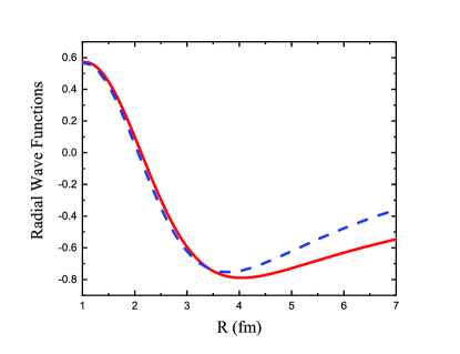
Figure 1: Solid red line: The radial wave function of the $(p{}^{12}{\rm C})_{2s_{1/2}^{+}}$ resonance state; dashed blue line: the radial wave function of the mirror $(n{}^{12}{\rm C})_{2s_{1/2}^{+}}$ bound-state. $r$ is the distance between $N$, where $N=p,n$, and the c.m. of ${}^{12}{\rm C}$.

Following the $R$-matrix procedure, both wave functions are normalized to unity over the internal volume with the radius $R_{ch}=4.0$ fm. We see that the mirror wave functions are very close at distances $\leq 4.0$ fm what confirms the mirror symmetry of $(p{}^{12}{\rm C})_{2s_{1/2}^{+}}$ and $(n{}^{12}{\rm C})_{2s_{1/2}^{+}}$ systems.

In Fig. 2 are shown the $\frac{{{\Gamma_{p{\,{}^{12}}{\rm{C}}}}}}{{{{({{C}_{n{\,{}^{12}}{\rm{C}}}})}^{2}}}}$ ratios, which are calculated using Eqs (79) and (82). These calculated ratios are compared with the experimental one. We see that the calculations exceed the experimental value. The $\frac{{{\Gamma_{p{\,{}^{12}}{\rm{C}}}}}}{{{{({{C}_{n{\,{}^{12}}{\rm{C}}}})}^{2}}}}$ ratio calculated using the simplified Eq. (82) shows the $R_{ch}$ dependence and is equal to $10.13\times 10^{-5}$ at the peak at $R_{ch}=5.22$ fm.

Equation (79) provides the $\frac{{{\Gamma_{p{\,{}^{12}}{\rm{C}}}}}}{{{{({{C}_{n{\,{}^{12}}{\rm{C}}}})}^{2}}}}$ ratio in terms of the ratio of the Wronskians. Each Wronskian contains the two-body wave function and its radial derivative of the system $(N\,{}^{12}{\rm C})_{2s_{1/2}^{+}}$, $N=p,n$. Each two-body wave function has one node at $r\approx 2.13$ fm and a minimum at $r\approx 4.0$ fm. . Hence, at some point $r$ the Wronskian in the denominator of Eq. (79) vanishes causing a discontinuity in the ratio $\frac{{{\Gamma_{p{\,{}^{12}}{\rm{C}}}}}}{{{{({{C}_{n{\,{}^{12}}{\rm{C}}}})}^{2}}}}$. I assume that in the nuclear interior the mirror two-body wave functions are correct (as it should be for the mirror microscopic overlap functions) and calculate the ratio at $E_{ch}\geq 4$ fm. At $r=4$ fm $\frac{{{\Gamma_{p{\,{}^{12}}{\rm{C}}}}}}{{{{({{C}_{n{\,{}^{12}}{\rm{C}}}})}^{2}}}}=8.1\times 10^{-5}$ while the correct value of this ratio obtained at large $R_{ch}$ is $9.8\times 10^{-5}$, which is close to the peak value of the ratio obtained using Eq. (82).

Both used equations provide the values of the $\frac{{{\Gamma_{p{\,{}^{12}}{\rm{C}}}}}}{{{{({{C}_{n{\,{}^{12}}{\rm{C}}}})}^{2}}}}$ ratio, which exceed the experimental one. It means that more accurate internal overlap functions are required and the two-body wave functions used here demonstrate the accuracy of the Wronskian method. However, there is another important conclusion: the simple Eq. (82) in the peak gives the same result as the asymptotic ratio given by Eq. (79).

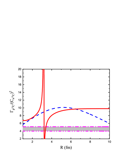
Figure 2: The grey band is the experimental $\frac{{{\Gamma_{p{\,{}^{12}}{\rm{C}}}}}}{{{{({{C}_{n{\,{}^{12}}{\rm{C}}}})}^{2}}}}$ ratio of the resonance width of the resonance state ${}^{13}{\rm N}(2s_{1/2}^{+})$ and the ANC of the mirror bound state ${}^{13}{\rm C}(2s_{1/2}^{+})$; the red dashed-dotted-dotted line and the red dashed-dotted lines are the low and upper limits of this experimental ratio; the solid red line is the $\frac{{{\Gamma_{p{\,{}^{12}}{\rm{C}}}}}}{{{{({{C}_{n{\,{}^{12}}{\rm{C}}}})}^{2}}}}$ ratio as a function of $R_{ch}$ calculated using Eq. (79); the blue dotted line is the $\frac{{{\Gamma_{p{\,{}^{12}}{\rm{C}}}}}}{{{{({{C}_{n{\,{}^{12}}{\rm{C}}}})}^{2}}}}$ ratio calculated as a function of $R_{ch}$ using Eq. (82).

V.2 Comparison of resonance width for $\mathbf{{}^{13}{\rm N}(1d_{5/2})\to{}^{12}{\rm C}(0.0\,{\rm MeV})+p}$ and mirror ANC for virtual decay $\mathbf{{}^{13}{\rm C}(1d_{5/2})\to{}^{12}{\rm C}(0.0\,{\rm MeV})+n}$

As the second example I consider the isobaric analogue states $1d_{5/2}$ in the mirror nuclei ${}^{13}{\rm N}$ and ${}^{13}{\rm C}$. The resonance energy of ${}^{13}{\rm N}(1d_{5/2})$ is $E_{p{}^{12}{\rm C}(0)}=1.6065$ MeV with the resonance width of $\Gamma_{p\,{}^{12}{\rm C}}=0.047\pm 0.0008$ MeV AjzenbergSelove . The neutron binding energy of the mirror state ${}^{13}{\rm C}(1d_{5/2})$ is $\varepsilon_{n{}^{12}{\rm C}}=1.09635$ MeV with the experimental ANC $C_{n{}^{12}{\rm C}}^{2}=0.0225$ fm^-1 liu . The experimental ratio is ${\Gamma_{{p\,^{12}}{\rm{C}}}}/C_{{n\,^{12}}{\rm{C}}}^{2}=(1.1\pm 0.2)\times{10^{-2}}$ .

In Fig. 3 are shown the radial wave functions of the mirror states.

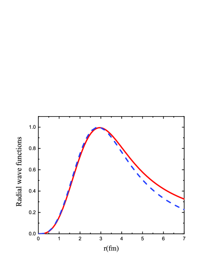
Figure 3: Solid red line: The radial wave function of the $(p{}^{12}{\rm C})_{1d_{5/2}^{+}}$ resonance state; dashed blue line: the radial wave function of the mirror $(n{}^{12}{\rm C})_{1d_{5/2}^{+}}$ bound-state. $r$ is the distance between $N$, where $N=p,n$, and the c.m. of ${}^{12}{\rm C}$.

Following the $R$-matrix procedure, both wave functions are normalized to unity over the internal volume with the radius $R_{ch}=3$ fm. We see that the mirror wave functions are very close at distances $r\leq 4$ fm what confirms the mirror symmetry of $(p{}^{12}{\rm C})_{1d_{5/2}^{+}}$ and $(n{}^{12}{\rm C})_{1d_{5/2}^{+}}$ systems.

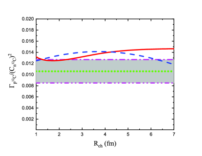
Figure 4: The grey band is the experimental $\frac{{{\Gamma_{p{\,{}^{12}}{\rm{C}}}}}}{{{{({{C}_{n{\,{}^{12}}{\rm{C}}}})}^{2}}}}$ ratio of the resonance width of the resonance state ${}^{13}{\rm N}(1d_{5/2}^{+})$ and the ANC of the mirror bound state ${}^{13}{\rm C}(1d_{5/2}^{+})$; the red dashed-dotted-dotted line and the red dashed-dotted lines are the low and upper limits of this experimental ratio; the green dotted line is the adopted experimental value of the ratio $\frac{{{\Gamma_{p{\,{}^{12}}{\rm{C}}}}}}{{{{({{C}_{n{\,{}^{12}}{\rm{C}}}})}^{2}}}}=(1.1\pm 0.2)\times{10^{-2}}$ ; the solid red line is the $\frac{{{\Gamma_{p{\,{}^{12}}{\rm{C}}}}}}{{{{({{C}_{n{\,{}^{12}}{\rm{C}}}})}^{2}}}}$ ratio as a function of $R_{ch}$ calculated using Eq. (79); the blue dotted line is the $\frac{{{\Gamma_{p{\,{}^{12}}{\rm{C}}}}}}{{{{({{C}_{n{\,{}^{12}}{\rm{C}}}})}^{2}}}}$ ratio calculated as a function of $R_{ch}$ using Eq. (82).

In Fig. 4 are shown the $\frac{{{\Gamma_{p{\,{}^{12}}{\rm{C}}}}}}{{{{({{C}_{n{\,{}^{12}}{\rm{C}}}})}^{2}}}}$ ratios calculated using Eqs (79) and (82), which are compared with the experimental ratio. We see that the calculated ratios are closer to the experimental ratio than in the previous case and both equations give quite reasonable results. The $\frac{{{\Gamma_{p{\,{}^{12}}{\rm{C}}}}}}{{{{({{C}_{n{\,{}^{12}}{\rm{C}}}})}^{2}}}}$ ratio calculated using the simplified Eq. (82) shows the $R_{ch}$ dependence and is equal to $0.0141$ at the peak at $R_{ch}=3.95$ fm. In the case under consideration the bound-state wave function does not have nodes at $r>0$. That is why the $\frac{{{\Gamma_{p{\,{}^{12}}{\rm{C}}}}}}{{{{({{C}_{n{\,{}^{12}}{\rm{C}}}})}^{2}}}}$ ratio calculated using Eq. (79) is a smooth function of $R_{ch}$ . This equation gives $\frac{{{\Gamma_{p{\,{}^{12}}{\rm{C}}}}}}{{{{({{C}_{n{\,{}^{12}}{\rm{C}}}})}^{2}}}}=0.0135$ at $R_{ch}=4$ fm, which differs very little from its correct asymptotic value of $0.0143$. Again, as in the previous case, our calculations show that the simple Eq. (82) can give the results close to the Wronskian method.

V.3 Comparison of resonance width for $\mathbf{{}^{15}{\rm F}(1d_{5/2})\to{}^{14}{\rm O}(0.0\,{\rm MeV})+p}$ and mirror ANC for virtual decay $\mathbf{{}^{15}{\rm C}(1d_{5/2})\to{}^{14}{\rm C}(0.0\,{\rm MeV})+n}$

In this section I determine the ratio ${\Gamma_{{p\,^{14}}{\rm{O}}}}/C_{{n\,^{14}}{\rm{C}}}^{2}$ for the mirror states ${}^{15}{\rm F}(1d_{5/2})$ and ${}^{15}{\rm C}(1d_{5/2})$. The resonance energy and the resonance width of ${}^{15}{\rm F}(1d_{5/2})$ are $E_{p{}^{14}{\rm O}(0)}=2.77$ MeV and $\Gamma_{p\,^{14}{\rm O}}=0.24\pm 0.03$ MeV Tilley . The binding energy and the ANC of the bound state ${}^{15}{\rm C}(1d_{5/2})$ are $\varepsilon_{n{}^{14}{\rm C}}=0.478$ MeV and $C_{n{}^{14}{\rm C}}^{2}=(3.6\pm 0.8)\times 10^{-3}$ fm^-1. The experimental ratio ${\Gamma_{{p\,^{14}}{\rm{O}}}}/C_{{n\,^{14}}{\rm{C}}}^{2}=0.338\pm 0.001$ .

This is the most difficult case because the resonance state is not potential. It is clear from Fig. 5.

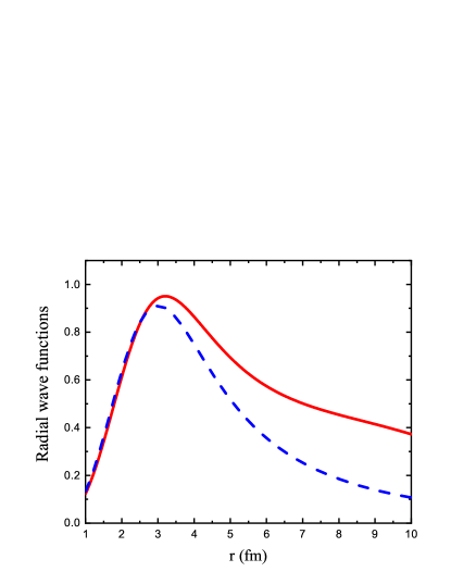
Figure 5: Solid red line: the radial wave function of the $(p{}^{14}{\rm O})_{1d_{5/2}}$ resonance state; dashed blue line: the radial wave function of the mirror $(n{}^{14}{\rm C})_{1d_{5/2}}$ bound-state. $r$ is the distance between the nucleon and the c.m. of the nucleus.

The mirror wave functions begin to deviate for $r>3.5$ fm. Because the resonance width in the case under consideration is much wider than in the previous cases, the calculated in the potential model resonant wave function in the external region differs significantly from the tail of the bound-state wave function. That is why the Wronskian ratio does not have an asymptote at large $r$. But the idea of the Wronskian method is to determine the ${\Gamma_{{p\,^{14}}{\rm{C}}}}/C_{{n\,^{14}}{\rm{C}}}^{2}$ ratio using the mirror wave functions in the internal region where they practically coincide.

In Fig. 6 is shown the ${\Gamma_{{p\,^{14}}{\rm{O}}}}/C_{{n\,^{14}}{\rm{C}}}^{2}$ ratio calculated using the Wronskian method and the simplified Eq. (82). The Wronskian ratio at $4.0$ fm is $0.32$ while Eq. (82) gives $0.31$. Both values are very close to the experimental ratio.

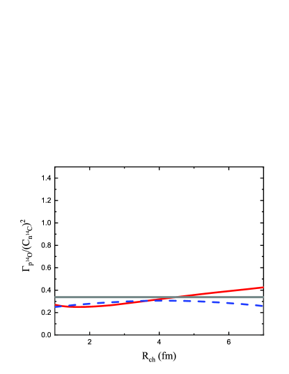
Figure 6: The grey band is the experimental $\frac{{{\Gamma_{p{\,{}^{14}}{\rm{O}}}}}}{{{{({{C}_{n{\,{}^{14}}{\rm{C}}}})}^{2}}}}$ ratio for the resonance state ${}^{15}{\rm F}(1d_{5/2}^{+})$ and the mirror bound state ${}^{15}{\rm C}(1d_{5/2}^{+})$; the solid red line is the $\frac{{{\Gamma_{p{\,{}^{14}}{\rm{O}}}}}}{{{{({{C}_{n{\,{}^{14}}{\rm{C}}}})}^{2}}}}$ ratio as a function of $R_{ch}$ calculated using Eq. (79); the blue dashed line is the $\frac{{{\Gamma_{p{\,{}^{14}}{\rm{O}}}}}}{{{{({{C}_{n{\,{}^{14}}{\rm{C}}}})}^{2}}}}$ ratio calculated as a function of $R_{ch}$ using Eq. (82).

V.4 Comparison of resonance width for $\mathbf{{}^{18}{\rm Ne}(1^{-})\to{}^{14}{\rm O}(0.0\,{\rm MeV})+\alpha}$ and mirror ANC for virtual decay $\mathbf{{}^{18}{\rm O}(1^{-})\to{}^{14}{\rm C}(0.0\,{\rm MeV})+\alpha}$

In this section I determine the ratio ${\Gamma_{{\alpha\,^{14}}{\rm{O}}}}/C_{{\alpha\,^{14}}{\rm{C}}}^{2}$ for the mirror states ${}^{18}{\rm Ne}(1^{-})$ and ${}^{18}{\rm O}(1^{-})$. The resonance energy is $E_{\alpha{}^{14}{\rm O}(0)}=1.038$ MeV . The binding energy of the bound state ${}^{18}{\rm O}(1^{-})$ is $\varepsilon_{\alpha{}^{14}{\rm C}}=0.027$ MeV. The resonance width and the ANC of the mirror states are unknown.

The purpose of this section is to show that the ratio ${\Gamma_{{\alpha\,^{14}}{\rm{O}}}}/C_{{\alpha\,^{14}}{\rm{C}}}^{2}$ does not depend on the number of the nodes of the mirror wave functions. The potential model search showed that for the given resonance energy and binding energy for $l=1$ the mirror wave functions have 4 or 6 nodes at $r>0$. In Figs 7 and 8 are shown the radial wave functions and the ratio ${\Gamma_{{\alpha\,^{14}}{\rm{O}}}}/C_{{\alpha\,^{14}}{\rm{C}}}^{2}$ for the number of the nodes $N=4$ and $6$.

One can see that the mirror wave functions practically coincide up to $r=15$ fm. It means that the simplified Eq. (82) can be used up to $15$ fm. The ratio ${\Gamma_{{\alpha\,^{14}}{\rm{O}}}}/C_{{\alpha\,^{14}}{\rm{C}}}^{2}$ calculated using Eq. (79) is the same for $N=4$ and $6$. Because the mirror wave functions practically identical in the external region the ratio ${\Gamma_{{\alpha\,^{14}}{\rm{O}}}}/C_{{\alpha\,^{14}}{\rm{C}}}^{2}$ calculated using the Wronskian method (Eq. (79)) has an asymptote. The calculated for $N=4,\,6$ ratio reaches its asymptotic value at $R_{ch}=7.5$ fm which is ${\Gamma_{{\alpha\,^{14}}{\rm{O}}}}/C_{{\alpha\,^{14}}{\rm{C}}}^{2}=3.48\,\times 10^{52}$. The maximum of ${\Gamma_{{\alpha\,^{14}}{\rm{O}}}}/C_{{\alpha\,^{14}}{\rm{C}}}^{2}$ calculated using Eq. (82) at $R_{ch}=9$ fm is $3.42\,\times 10^{52}$. This comparison demonstrates again that in the absence of the microscopic internal overlap functions both the Wronskian and the simplified method given by Eq. (82) can be used and give very close results.

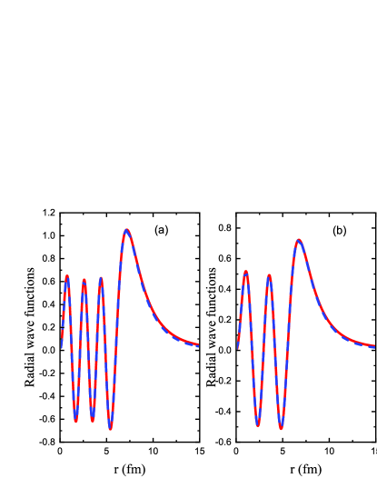
Figure 7: Panel (a): the mirror radial wave functions for $N=6$; the solid red line is the $(\alpha{}^{14}{\rm O})_{1^{-}}$ resonance wave function; the dashed blue line is the radial wave function of the mirror $(\alpha{}^{14}{\rm C})_{1^{-}}$ bound-state. $r$ is the distance between the $\alpha$-particle and the c.m. of the nucleus. Panel (b): notations are the same as in panel (a) but for $N=4$.

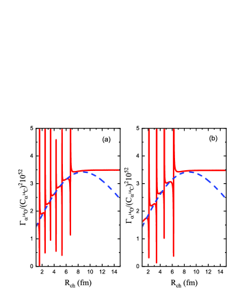
Figure 8: Panel (a): the $\frac{{{\Gamma_{\alpha{\,{}^{14}}{\rm{O}}}}}}{{{{({{C}_{\alpha{\,{}^{14}}{\rm{C}}}})}^{2}}}}$ ratio for the resonance state ${}^{18}{\rm Ne}(1^{-})$ and the mirror bound state ${}^{18}{\rm O}(1^{-})$ for $N=6$; the solid red line is the $\frac{{{\Gamma_{\alpha{\,{}^{14}}{\rm{O}}}}}}{{{{({{C}_{\alpha{\,{}^{14}}{\rm{C}}}})}^{2}}}}$ ratio as a function of $R_{ch}$ calculated using Eq. (79); the blue dashed line is the $\frac{{{\Gamma_{\alpha{\,{}^{14}}{\rm{O}}}}}}{{{{({{C}_{\alpha{\,{}^{14}}{\rm{C}}}})}^{2}}}}$ ratio calculated as a function of $R_{ch}$ using Eq. (82). Panel (b): notations are the same as in panel (a) but for $N=4$.

V.5 Comparison of resonance width for $\mathbf{{}^{17}{\rm F}(s_{1/2})\to{}^{13}{\rm N}(0.0\,{\rm MeV})+\alpha}$ and mirror ANC for virtual decay $\mathbf{{}^{17}{\rm O}(s_{1/2})\to{}^{13}{\rm C}(0.0\,{\rm MeV})+\alpha}$

The last case, which I consider, is the determination of the ratio $\frac{{{\Gamma_{\alpha{\,{}^{13}}{\rm{N}}}}}}{{{{({{C}_{\alpha{\,{}^{13}}{\rm{C}}}})}^{2}}}}$ of the resonance state ${}^{17}{\rm F}(1/2^{+})$ and the mirror bound state ${}^{17}{\rm O}(1/2^{+})$. The orbital momentum of the mirror states is $l=1$ and the resonance energy is $E_{\alpha\,{}^{13}{\rm N}(0)}=0.7371$ MeV Tilley . The location of the state ${}^{17}{\rm O}(1/2^{+})$ is questionable. The excitation energy $E_{x}$ of the state ${}^{17}{\rm O}(1/2^{+})$ is $6356\pm 8$ keV Tilley . Taking into account that the $\alpha-{}^{13}{\rm C}$ threshold is located at $6359.2$ keV one finds that this $1/2^{+}$ level is the located at $E_{\alpha{}^{13}{\rm C}}=-3\pm 8$ keV, that is, it can be a subthreshold bound state or a resonance Tilley . This location of the level ${}^{17}{\rm O}(1/2^{+})$ was adopted in the previous analyses of the direct measurements including the latest one in Heil . If this level is the subthreshold bound state, then its reduced width is related to the ANC of this level. However, in a recent paper Faestermann it has been determined that this level is actually a resonance located at $E_{\alpha{}^{13}{\rm C}}=4.7\pm 3$ keV. Because the possible subthreshold state and near threshold resonance are located very close to each other the reduced widths corresponding to these two levels are very close. Here in the analysis I still assume that ${}^{17}{\rm O}(1/2^{+})$ is the bound state with the binding energy of $-3$ keV. I adopt the ANC of this subthreshold state $C_{\alpha{}^{13}{\rm C}}^{2}=4.4\times 10^{169}$ fm^-1 muk2017 .

The calculated mirror resonance and bound state wave functions are shown in Fig. 9. Both wave functions practically identical up to $R_{ch}\leq 15$ fm.

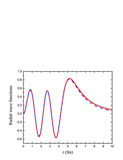
Figure 9: The solid red line is the $(\alpha{}^{13}{\rm N})_{1/2^{+}}$ resonance wave function; the dashed blue line is the radial wave function of the mirror $(\alpha{}^{13}{\rm C})_{1/2^{+}}$ bound-state. $r$ is the distance between the $\alpha$-particle and the c.m. of the nucleus.

In Fig. 10 the $\frac{{{\Gamma_{\alpha{\,{}^{13}}{\rm{N}}}}}}{{{{({{C}_{\alpha{\,{}^{13}}{\rm{C}}}})}^{2}}}}$ ratio is calculated using the Wronskian Eq. (79) and the simple Eq. (82). The asymptotic value of the ratio is $\frac{{{\Gamma_{\alpha{\,{}^{13}}{\rm{N}}}}}}{{{{({{C}_{\alpha{\,{}^{13}}{\rm{C}}}})}^{2}}}}=4.48\times 10^{-178}$. The value of the $\frac{{{\Gamma_{\alpha{\,{}^{13}}{\rm{N}}}}}}{{{{({{C}_{\alpha{\,{}^{13}}{\rm{C}}}})}^{2}}}}$ at the border of the internal region $R_{ch}=5.2$ fm is very close to its asymptotic value. Eq. (82) gives $\frac{{{\Gamma_{\alpha{\,{}^{13}}{\rm{N}}}}}}{{{{({{C}_{\alpha{\,{}^{13}}{\rm{C}}}})}^{2}}}}=4.55\times 10^{-178}$. Taking into account the adopted value of the ANC $C_{\alpha\,{}^{13}{\rm C}}$ and the experimental ratio $\frac{{{\Gamma_{\alpha{\,{}^{13}}{\rm{N}}}}}}{{{{({{C}_{\alpha{\,{}^{13}}{\rm{C}}}})}^{2}}}}=4.48\times 10^{-178}$ one obtains from the Wronskian ratio the resonance width $\Gamma_{\alpha\,{}^{13}N}=4.48\times 10^{-178}\times 4.4\times 10^{169}\,\times\hbar\,c=3.9$ eV.

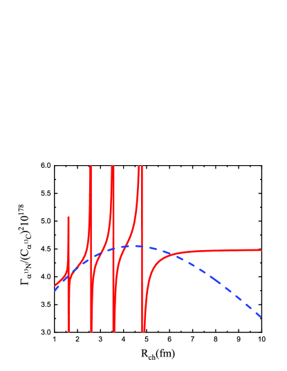
Figure 10: The $\frac{{{\Gamma_{\alpha{\,{}^{13}}{\rm{N}}}}}}{{{{({{C}_{\alpha{\,{}^{13}}{\rm{C}}}})}^{2}}}}$ ratio for the resonance state ${}^{17}{\rm F}(1/2^{+})$ and the mirror bound state ${}^{17}{\rm O}(1/2^{+})$; the solid red line is the $\frac{{{\Gamma_{\alpha{\,{}^{13}}{\rm{N}}}}}}{{{{({{C}_{\alpha{\,{}^{13}}{\rm{C}}}})}^{2}}}}$ ratio as a function of $R_{ch}$ calculated using Eq. (79); the blue dashed line is the $\frac{{{\Gamma_{\alpha{\,{}^{13}}{\rm{N}}}}}}{{{{({{C}_{\alpha{\,{}^{13}}{\rm{C}}}})}^{2}}}}$ ratio calculated as a function of $R_{ch}$ using Eq. (82).

VI Appendix

In this Appendix is shown that Zeldovich regularization procedure can be used for normalization of the resonance wave function $u_{k_{p}l_{B}}(r)$ both for exponentially decaying potentials and potentials with the Coulomb tail. The normalization of the resonance wave function depends on its tail. Taking into account Eq. (13) it is enough to consider the integral

$$I(\beta,\nu,z)=\int\limits_{0}^{\infty}{\rm d}r\,e^{-\beta\,r^{2}}\,e^{z\,r}\,r^{\nu}.$$ (83)

Here, $\;z=2\,i\,k_{aA(R)}\,r=2\,i\,k_{aA(0)}\,r+2\,{\rm Im}{k_{aA(R)}}\,r$. It assumed that $k_{aA(0)}>{\rm Im}{k_{aA(R)}}$, as it should be for physical resonances. Then ${\rm Re}z^{2}<0$. Also

$$\nu=-2\,i\,\eta_{aA}^{R}=-2i\,\frac{\gamma}{k_{aA(0)}-i\,{\rm Im}\,{k_{aA(R)}}}=-2\,i\,\frac{\gamma\,(k_{aA(0)}}{k_{aA(0)}^{2}+({\rm Im}{k_{aA(R)}})^{2}}+2\,\frac{\gamma\,{\rm Im}{k_{aA(R)}}}{k_{aA(0)}^{2}+({\rm Im}{k_{aA(R)}})^{2}},$$ (84)

$\gamma=Z_{a}\,Z_{A}\,\mu_{aA}/137$. Thus, one can see that for the repulsive Coulomb potential ${\rm Re}\nu>0$.

Using Eq. (3.462.1) from GradRyzhik one gets

$$I(\beta,\nu,z)=\Gamma(\nu+1)\,(2\,\beta)^{-(\nu+1)/2}\,e^{z^{2}/(8\,\beta)}\,D_{-\nu-1}(-z/\sqrt{2\,\beta}),$$ (85)

where $D_{\sigma}(x)$ is the parabolic cylinder function. For ${\rm Re}z^{2}<0$ using Eq. (9.246.1) from GradRyzhik one gets

$$I(0,\,\nu,\,z)=\lim_{\beta\to+0}\,I(\beta,\,\nu,\,z)=\Gamma(\nu+1)\,(-z)^{-\nu-1}.$$ (86)

Thus the regularization procedure used by Zeldovich is applicable and for the physical resonances $\,k_{aA(0)}>{\rm Im}{k_{aA(R)}}\,$ the integral in Eq. (83) does exist and converges in the $\lim\,{\beta\to+0}$ .

Let me consider now the integral

$$I_{R}(\beta,\nu,z)=\int\limits_{R}^{\infty}{\rm d}r\,e^{-\beta\,r^{2}}\,e^{z\,r}\,r^{\nu}.$$ (87)

Integrating it by parts one gets

$$\lim_{\beta\to+0}\,I_{R}(\beta,\nu,z)=-\frac{R^{\nu}}{z}\,e^{z\,R}\,\Big{[}1-\frac{\nu}{z\,R}+O(\frac{1}{z^{2}\,R^{2}})\Big{]}.$$ (88)

VII acknowledgments

This work was supported by the U.S. DOE Grant No. DE-FG02-93ER40773, NNSA Grant No. DE-NA0003841 and U.S. NSF Award No. PHY-1415656.

References

- (1) L. D. Blokhintsev, I. Borbely, and E. I. Dolinskii, Fiz. Elem. Chastits t. Yadra 8, 1189 (1977) [Sov. J. Part. Nucl. 8, 485 (1977)].
- (2) L. D. Blokhintsev, A. M. Mukhamedzhanov, A. N. Safronov, Fiz. Elem. Chastits t. Yadra 15, 1296 (1984) [Sov. J. Part. Nucl. 15, 580 (1984)].
- (3) A. M. Mukhamedzhanov and N. K. Timofeyuk, Pis’ma Eksp. Teor. Fiz. 51, 247 (1990) [JETP Lett. 51, 282 (1990)].
- (4) A. M. Mukhamedzhanov, C. A. Gagliardi, and R. E. Tribble, Phys. Rev. C 63, 024612 (2001) .
- (5) A. M. Mukhamedzhanov, L. D. Blokhintsev, and B. F. Irgaziev, Phys. Rev. C 83, 055805 (2011).
- (6) A. M. Mukhamedzhanov and N. K. Timofeyuk, Sov. J. Nucl. Phys. 51, 431 (1990) [Yad. Fiz. 51, 679 (1990)].
- (7) Xiaodong Tang, A. Azhari, C. A. Gagliardi, A. M. Mukhamedzhanov, F. Pirlepesov, L. Trache, R. E. Tribble, V. Burjan, V. Kroha, and F. Carstoiu, Phys. Rev. C 67, 015804 (2003).
- (8) A. M. Mukhamedzhanov, M. La Cognata and V. Kroha, Phys. Rev. C 83, 044604 (2011).
- (9) A. M. Mukhamedzhanov and R. E. Tribble, Phys. Rev. C 59, 3418 (1999).
- (10) N. K. Timofeyuk, R. C. Johnson, and A. M. Mukhamedzhanov, Phys. Rev. Lett. 91, 232501 (2003).
- (11) A. M. Mukhamedzhanov, Phys. Rev. C 86, 044615 (2012).
- (12) H. . Kramers, Hand und Jahrbuch der Chemischer Physik 1, 312 (1938).
- (13) W. Heisenberg, Zs f. Naturforsch. 1, 608 (1946).
- (14) C. Möller, Dan. Vid Selsk. Mat. Fys. Medd. 22, N.19 (1946).
- (15) N. Hu, Phys. Rev. 74, 131 (1948).
- (16) Ya. B. Zel’dovich, ZhetF 51, 1492 (1965).
- (17) M. Perelomov, V.S. Popov, M. V. Terent ev, ZhETF 51, 309 (1966).
- (18) W. T. Pinkston and G. R. Satchler, Nucl. Phys. 72, 641 (1965)
- (19) R. J. Philpott, W. T. Pinkston, and G. R. Satchler, Nucl. Phys. A119, 241 (1968).
- (20) N.K. Timofeyuk, Nucl. Phys. A632, 19 (1998).
- (21) R. G. Newton, Scattering Theory of Waves and Particles, 2nd ed., Springer-Verlag, Heidelberg, 1982.
- (22) P. Navratil, J. P. Vary and B. R. Barrett, Phys. Rev. C 62, 054311 (2000).
- (23) P. Navratil, W. E. Ormand, Phys. Rev. C 68, 034305 (2003).
- (24) S. Quaglioni, P. Navratil, Phys. Rev. Lett. 101, 092501 (2008).
- (25) O. Jensen, G. Hagen, M. Hjorth-Jensen, B. A. Brown, A. Gade, Phys. Rev. Lett. 107, 032501 (2011).
- (26) N. K. Timofeyuk, Phys. Rev. C 84, 054313 (2011).
- (27) F. Ajzenberg-Selove, Nucl. Phys. A523, 1 (1991).
- (28) Z. H. Liu et al., Phys. Rev. C 64, 034312 (2001).
- (29) N. Imai et al., Nucl. Phys. A688, 281c (2001).
- (30) D. R. Tilley, H. R. Weller, and C. M. Cheves, Nucl. Phys. A564, 1 (1993).
- (31) M. Heil, R. Detwiler, and R. E. Azuma et al., Phys. Rev. C 78, 025803 (2008).
- (32) T. Faestermann, P. Mohr, R. Hertenberger, and H.-F. Wirth, Phys. Rev. C 92, 052802(R) (2015).
- (33) A. M. Mukhamedzhanov, Shubhchintak, and C. A. Bertulani, Phys. Rev. C 96, 024623 (2017) .
- (34) I. S. Gradshteyn and L/ M. Ryzhik, Tables of Integrals, Series and Products, Academic Press, New York, London, 1980.