Linear Whitham-Boussinesq modes in channels of constant cross-section.

Abstract

We study normal modes for the linear water wave problem in infinite straight channels of bounded constant cross-section. Our goal is to compare semi-analytic normal mode solutions known in the literature for special triangular cross-sections, namely isosceles triangles of equal angle of $45^{\circ}$ and $60^{\circ}$, see Lamb lamb1932hydrodynamics , Macdonald macdonald1893waves , Greenhill greenhill1887wave , Packham packham1980small , and Groves groves1994hamiltonian , to numerical solutions obtained using approximations of the non-local Dirichlet-Neumann operator for linear waves, specifically an ad-hoc approximation proposed in vargas2016whitham , and a first order truncation of the systematic depth expansion by Craig, Guyenne, Nicholls and Sulem CGNS . We consider cases of transverse (i.e. 2-D) modes and longitudinal modes, i.e. 3-D modes with sinusoidal dependence in the longitudinal direction. The triangular geometries considered have slopping beach boundaries that should in principle limit the applicability of the approximate Dirichlet-Neumann operators. We nevertheless see that the approximate operators give remarkably close results for transverse even modes, while for odd transverse modes we have some discrepancies near the boundary. In the case of longitudinal modes, where the theory only yields even modes, the different approximate operators show more discrepancies for the first two longitudinal modes and better agreement for higher modes. The ad-hoc approximation is generally closer to exact modes away from the boundary.

1 Introduction

We study some problems on normal modes in the linear water wave theory, in particular we compute transverse and longitudinal normal modes in infinite straight channels of constant bounded cross-section, considering special depth profiles for which there are known explicit or semi-explicit analytical solutions in the literature greenhill1887wave ; groves1994hamiltonian ; lamb1932hydrodynamics ; macdonald1893waves ; packham1980small . We compare the results to numerical normal modes obtained by using simple approximations of the nonlocal variable depth Dirichlet-Neumann operator for the linear water wave equations, in particular a recently proposed ad-hoc approximation vargas2016whitham , as well as a first order truncation of the systematic expansion in the depth proposed by Craig, Guyenne, Nicholls and Sulem CGNS . Our main motivation is to test the simple approximations to the Dirichlet-Neumann operator as they are of interest in constructing simplified nonlocal shallow water models, e.g. Whitham-Boussinesq equations AcevesSanchez201380 ; Carter2018 ; HurTao2018 ; moldabayev2014whitham and arXiv:1608.04685 submitted manuscript by V. M. Hur and A. K. Pandey. Such models have attracted considerable current interest constantin1998wave ; ehrnstrom2009traveling ; ehrnstrom2012existence ; hur2015breaking ; naumkin1994nonlinear and arXiv:1602.05384 submitted manuscript by M. Ehrnstrom and E. Wahlén. The inclusion of variable depth effects raises additional questions on the dynamics of these systems and is of interest in geophysical and coastal engineering applications.

The nonlocal linear system we use to compute normal modes is derived using the Hamiltonian formulation of the free surface potential flow zakharov1968stability , see also miles1977hamilton ; radder1992explicit , and approximations for the (nonlocal) Dirichlet-Neumann operators for the Laplacian in the fluid domain appearing in the kinetic energy part of the Hamiltonian craig1994hamiltonian . Explicit infinite series expressions for the Dirichlet-Neumann operator in variable depth were derived by Craig, Guyenne, Nicholls and Sulem CGNS , see also lannes2013water . Such expressions are generally complicated and can be used for numerical computations gouin2015development , or to further simplify the equations of motion. The Hamiltonian and Dirichlet-Neumann formulation implies that variable depth effects are already captured at the level of the linear theory, i.e. the nontrivial wave-amplitude operator is expressed recursively in terms of the linear operator craig1993numerical ; CGNS . The study of linear normal modes is therefore a good test problem for comparing different approximations of the Dirichlet-Neumann operator for variable depth. In this paper we focus on simple approximations of the variable depth operator, such as the ad-hoc generalization of the constant depth operator for arbitrary depth proposed in vargas2016whitham . This operator has some of the structural properties of the exact Dirichlet-Neumann operator, e.g. symmetry and exact infinite depth asymptotics, but is also seen to lead to a depth expansion that differs from the exact one of CGNS .

The idea of the paper is compare results obtained using the approximate Dirichlet-Neumann operators to semi-analytic normal mode solutions known for some special depth profiles. These analytical results rely on the existence of families of harmonic functions that satisfy the rigid wall boundary conditions at the bottom, and can be only obtained for a few special depth profiles, such as isosceles triangles with sides inclined at $45^{\circ}$ and $60^{\circ}$ to the vertical, see Greenhill greenhill1887wave , Macdonald macdonald1893waves , and the summary in Lamb’s book, lamb1932hydrodynamics . More recent studies are by Packham packham1980small and Groves groves1994hamiltonian . A complete set of modes was also obtained for a semicircular channel by Evans and Linton evans1993sloshing . The construction typically yields even and odd normal modes that we then compare to even and odd eigenfunctions of approximate Dirichlet-Neumann operators in a periodic domain.

One problem with our plan is that the non-constant depth examples with classical analytic solutions we are aware of concern domains with a slopping beach, and as we clarify below, the classical and periodic Dirichlet-Neumann approaches are not equivalent because of the different assumptions at the intersection between the horizontal and sloping beach boundaries. Despite this problem, we find that the two approaches give comparable and often very close results for the 2-D normal mode shapes, especially away from the beach. This is especially the case for even modes, where we see good agreement in the entire domain. Results for odd modes are close away from the beach, but have a marked discrepancy near the beach. In that case the periodic problem for the approximate Dirichlet-Neumann operators leads to modes with that vanish at boundary, while odd exact modes have maxima at the boundary. In the problem of 3-D even longitudinal modes, we consider moderate speed along the transverse direction and see more discrepancies between the exact and approximate modes. Agreement in the interior is good after the first two modes, but discrepancies at the boundary persist for higher even modes. The approximate Dirichlet-Neumann approach also gives results for the odd case, where there are no exact results.

In summary, the approximate periodic Dirichlet-Neumann operators give better results for the transverse 2-D modes, especially in the interior. In Section 4 we present evidence that the modes computed by the approximate periodic Dirchlet-Neumann operators are limiting cases of modes corresponding to a periodic depth profiles with nowhere vanishing depth. This observation explains intuitively why the approximate operators can not capture the slopping beach rigid wall boundary condition as realistically as the classical exact approach.

The organization of the paper is as follows. In Section 2 we formulate the water wave problem using the Dirichlet-Neumann operators and present the operators used to approximate the linear system. In Section 3 we formulate the classical problem of transverse and longitudinal modes for the linear theory and define analogues that use approximate Dirichlet-Neumann operators. In Section 4 we present our results, comparing normal modes obtained using the classical and approximate Dirichlet-Neumann approaches. In Section 5 we briefly discuss the results.

2 Water wave problem in variable depth and approximate Dirichlet-Neumann operators

Following the Hamiltonian formulation of the water wave problem due to Zakharov zakharov1968stability , see also miles1977hamilton ; radder1992explicit , the Euler equations for free surface potential flow can be restated as a Hamiltonian system in terms of the wave amplitude $\eta(x,t)$ and surface hydrodynamic potential $\xi(x,t)=\varphi(x,\eta(x,t),t),$ namely as

$$\partial_{t}\left(\begin{array}[]{l}\eta\\ \xi\\ \end{array}\right)=\left(\begin{array}[]{cc}0&I\\ -I&0\end{array}\right)\left(\begin{array}[]{l}\frac{\delta H}{\delta\eta}\\ \frac{\delta H}{\delta\xi}\\ \end{array}\right),$$ (1)

where the Hamiltonian is expressed explicitly in terms of $\eta$ and $\xi$ as

$$H=\frac{1}{2}\int_{\mathbb{R}}(\xi G(\beta,\eta)\xi+g\eta^{2})dx,$$ (2)

see craig1994hamiltonian , and the operator $G(\beta,\eta)$ is defined as follows: consider the elliptic problem

$$\Delta\varphi(x,y)=0, \forall\text{ }(x,y)\in\mathcal{D}_{t}(\eta)$$ (3)

$$\varphi(x,\eta(x))=\xi(x), \forall\text{ }x\in\mathbb{R},$$ (4)

$$\frac{\partial\varphi}{\partial\hat{n}}(x,-h_{0}+\beta(x))=0, \forall\text{ }x\in\mathbb{R},$$ (5)

in the two dimensional (time-dependent) simply connected domain $\mathcal{D}_{t}(\eta):=\{(x,y):x\in\mathbb{R},-h_{0}+\beta(x)<y<\eta(x,t)\}$. If $\eta$ and $\xi$ are sufficiently smooth and decay at infinity then (3)-(5) admits a unique solution and we can compute the normal derivative of the solution at the surface $y=\eta$. The Dirichlet-Neumann operator $G(\beta,\eta)$ is then defined by

$$(G(\beta,\eta)\xi)(x)=(1+(\partial_{x}\eta(x))^{2})^{\frac{1}{2}}\triangledown\varphi(x,\eta(x))\cdot N(\eta(x)),$$ (6)

where $N(\eta(x))=(1+(\partial_{x}\eta(x))^{2})^{-\frac{1}{2}}(-\partial_{x}\eta(x),1)$, $x\in\mathbb{R}$, is the exterior unit normal at the free surface. The Dirichlet-Neumann operator $G(\beta,\eta)$ is a linear operator on $\xi$ and is symmetric with respect to the usual $L^{2}$ inner product. Similar definitions apply to the periodic problem and to higher dimensions.

In CGNS , Craig, Guyenne, Nicholls and Sulem give an expansion of this operator in the presence of non-trivial bottom topography

$$G(\beta,\eta)=G_{0}(\beta,\eta)+G_{1}(\beta,\eta)+G_{2}(\beta,\eta)+...,$$ (7)

where the $G_{j}$ are homogeneous of degree $j$ in $\eta.$ The first terms are

$$G_{0}(\beta,\eta) = D\tanh(h_{0}D)+DL(\beta),$$ (8)

$$G_{1}(\beta,\eta) = D\eta D-G_{0}\eta G_{0},$$ (9)

$$G_{2}(\beta,\eta) = \frac{1}{2}(G_{0}D\eta^{2}D-D^{2}\eta^{2}G_{0}-2G_{0}\eta G_{1}),$$ (10)

where $D=-i\partial_{x}$, and $G_{0}=G_{0}[\beta,\eta]$. We are also using the notation

$$[a(f(x)D^{m})\xi](x)=\frac{1}{2\pi}\int_{\mathbb{R}}a(f(x)k^{m})\hat{\xi}(k)e^{ikx}dk,$$ (11)

with $a$, $f$ be real functions, and $\hat{\xi}(k)=\int_{\mathbb{R}}\xi(x)e^{-ikx}dk$, the Fourier transform of the real function $\xi$.

At higher order, the $G_{j}$, $j>2$, are similarly obtained from $G_{0}$, using a recursion formula. The recursion formula for the $G_{j}$ is similar to the one obtained for a flat bottom, where $G_{0}=D\tanh(h_{0}D)$, see craig1993numerical . Variable depth effects are thus encoded in the operator $L(\beta)$.

The operator $L(\beta)$ can be expressed in powers of the depth variation $\beta$ as $L(\beta)=\Sigma_{j=0}^{\infty}L_{j}(\beta),$ where the $L_{j}(\beta)$ are homogeneous of order $j$ in $\beta$, and are computed recursively, see CGNS . The first two terms in the expansion are

$$L_{0}(\beta) = 0,$$ (12)

$$L_{1}(\beta) = -\text{sech}(h_{0}D)\beta D\text{sech}(h_{0}D).$$ (13)

The first two terms of this expansion lead the first order approximation $\mathcal{A}_{1}$ of the Dirichlet-Neumann operator

$$\mathcal{A}_{1}(\beta)=D\tanh(h_{0}D)-D\text{sech}(h_{0}D)\beta D\text{sech}(h_{0}D)$$ (14)

that we use below. This operator was used recently by W. Craig, M. Gazeau, C. Lacave, C. Sulem to calculate bands for periodic depth variation see arXiv:1706.07417 submitted manuscript.

Higher order expansions in $\beta$ have been considered in the numerical study of gouin2015development . To avoid these longer expressions in simplified nonlocal shallow water equations, vargas2016whitham proposed an ad-hoc approximation $\mathcal{A}_{G_{0}}$ of the linear Dirichlet-Neumann operator given by

$$\mathcal{A}_{G_{0}}(\beta)=\textit{Sym}(D\tanh(h(x)D)),$$ (15)

where $h(x)=h_{0}-\beta(x)$. The (formal) symmetrization of a linear operator $\mathcal{A}$ in $L^{2}=L^{2}(\mathbb{R};\mathbb{R})$ with the (standard) inner product $\langle f,g\rangle=\int_{\mathbb{R}}f(x)g(x)dx$, is defined by $\textit{Sym}(\mathcal{A})=\frac{1}{2}(\mathcal{A}+\mathcal{A}^{*})$, where $\mathcal{A}^{*}$ is the adjoint of $\mathcal{A}$ with respect to the inner product, i.e. $\langle\mathcal{A}f,g\rangle=\langle f,\mathcal{A}^{*}g\rangle$, for all $f$, $g$ in the the domains of $\mathcal{A}$, $\mathcal{A}^{*}$ respectively. (It is assumed that the domain $D(\mathcal{A})$ of $\mathcal{A}$ is dense in $L^{2}$.) $\mathcal{A}$ is symmetric if $D(\mathcal{A})=D(\mathcal{A}^{*})$ and $\mathcal{A}=\mathcal{A}^{*}$, thus $D(\mathcal{A})=D(\mathcal{A}^{*})$ implies that $\textit{Sym}(\mathcal{A})$ is symmetric.

Symmetrizing an approximate Dirichlet-Neumann operator is natural by (1), (2), e.g. $H=\frac{1}{2}\int_{\mathbb{R}}(\xi\mathcal{A}\xi+g\eta^{2})$, $\mathcal{A}$ a linear operator, leads formally to the equations ${\partial_{t}\eta}=\frac{1}{2}(\mathcal{A}+\mathcal{A}^{*})\xi$, ${\partial_{t}\xi}=-g\eta$. We note that $D\tanh(h(x)D)$ maps real-valued functions to real-valued functions, see Appendix A and the next section for further details on symmetrizing this operator.

We check that $\mathcal{A}_{1}(\beta)$ of (14) is symmetric. To compare this operator to $\mathcal{A}_{G_{0}}$, we expand $D\tanh(h(x)D)$ in $\beta$ to $O(\beta^{2})$, and symmetrize. The result is the operator

$$\mathcal{A}_{2}(\beta) = D\tanh(h_{0}D)+\frac{1}{2}[i\beta^{\prime}\text{sech}^{2}(h_{0}D)D-\beta\text{sech}^{2}(h_{0}D)D^{2}$$

$$-iD\text{sech}^{2}(h_{0}D)\beta^{\prime}+D^{2}\text{sech}^{2}(h_{0}D)\beta],$$

see Appendix A. We see that operators $\mathcal{A}_{1}$ and $\mathcal{A}_{2}$ are apparently different.

As was pointed out in CGNS , the formulation can be extended to 3-D domains. Recently in andrade2018three a Dirichlet-Neumann operator for a three-dimensional surface water wave problem in the presence of highly variable, non smooth topagraphy is constructed using a Galerkin method in Fourier space.

Let $a$, $f$ be real functions and $g:{\mathbb{R}}^{2}\rightarrow{\mathbb{R}}$, and let $D=(D_{1},D_{2})^{T}=-i(\partial_{x_{1}},\partial_{x_{2}})^{T}$. We then define operators $a(f(x)g(D))$ by

$$[a(f(\mathbf{x})g(D))\xi](\mathbf{x})=\frac{1}{(2\pi)^{2}}\int_{\mathbb{R}^{2}}a(f(\mathbf{x})g(\mathbf{k}))\hat{\xi}(\mathbf{k})e^{i\mathbf{k}\cdot\mathbf{x}}d^{2}\mathbf{k},$$ (17)

with ${\hat{\xi}}(\mathbf{k})=\int_{\mathbb{R}^{2}}{\xi}(\mathbf{x})e^{-i\mathbf{k}\cdot\mathbf{x}}d^{2}{\mathbf{x}}$, the Fourier transform of the function $\xi$ on ${\mathbb{R}}^{2}$.

Letting

$$\left|D\right|=\sqrt{\left|D_{1}\right|^{2}+\left|D_{2}\right|^{2}},$$ (18)

the expansion of $L(\beta)$ up to $O(\beta^{2})$ leads to the approximate Dirichlet-Neumann operator

$$\mathcal{A}_{1}(\beta)=[\left|D\right|\tanh(h_{0}\left|D\right|)]-[\left|D\right|\text{sech}(h_{0}\left|D\right|)][\beta(\textbf{x})\left|D\right|\text{sech}(h_{0}\left|D\right|)].$$ (19)

We will also consider the 3-D analogue of the ad-hoc operator of (15)

$$\mathcal{A}_{G_{0}}(\beta)=\textit{Sym}[\left|D\right|\tanh(h(\mathbf{x})\left|D\right|)],\text{ }\text{}$$ (20)

with $h(\mathbf{x})=h_{0}-\beta(\mathbf{x})$. The symmetrization is defined as in $\mathbb{R}$.

3 Linear modes in channels and
Dirichlet-Neumann operators

We now consider the classical formulation of the problem of linear modes in channels. We use Cartesian coordinates denoted by $(x,y,z)$, where $y$ is directed vertically upwards, $x$ is measured longitudinally along the channel and $z$ is measured across the channel, see e.g. Figure 3 and 9

We define the fluid domain as $\mathcal{D}=\mathbb{R}\times\Omega,$ where $\Omega\subset\mathbb{R}^{2}$ is the cross section. We assume a bounded cross sections $\Omega=\Omega_{B}$ of the form

$$\Omega_{B}=\{[z,y]:z\in[0,b],y\in[h_{m}+\beta(z),h_{M}],$$ (21)

The heights $y=h_{m}$ and $y=h_{M}$ describe the minimum and maximum elevations of the fluid domain respectively, with $h_{m}<h_{M}$, and $h_{m}+\beta(z)\leq h_{M}$ for all $z$.

We will assume $\partial\mathcal{D}=\mathbb{R}\times\partial\Omega=\Gamma_{L}\cup\Gamma_{F}\cup\Gamma_{B}$, with $\Gamma_{L}$ representing the lateral wall, $\Gamma_{F}$ representing the free surface, and $\Gamma_{B}$ the bottom,

$$\Gamma_{F}=\{(x,h_{M},z):x\in\mathbb{R},0\leq z\leq b\},$$ (22)

$$\Gamma_{B}=\{(x,h_{m}+\beta(z),z):x\in\mathbb{R},0\leq z\leq b\},$$ (23)

$$\Gamma_{L}=\{(x,y,0):x\in\mathbb{R},y\in[h_{m}+\beta(0),h_{M}]\}\cup\{(x,y,b):x\in\mathbb{R},y\in[h_{m}+\beta(b),h_{M}]\}.$$ (24)

In this article we are interested in domains with $h_{m}+\beta(z)=h_{M}$ at $z=0$ and $z=b$. Then $\Gamma_{L}=\emptyset$.

To state the problem we introduce a velocity potential $\phi(x,y,z,t)$ and look for solutions of Laplace’s equation

$$\phi_{xx}+\phi_{yy}+\phi_{zz}=0\text{ in }\mathcal{D,}$$ (25)

with

$$\left\{\begin{array}[]{l}\phi_{t}+g\eta=0\text{ at }\Gamma_{F},\\ \eta_{t}=\phi_{y}\text{ at }\Gamma_{F},\\ \frac{\partial\phi}{\partial{\hat{n}}}=0\text{ at }\Gamma_{B}\cup\Gamma_{L},\end{array}\right.$$ (26)

see whitham2011linear . Equations (25), (26) are the linearized Euler equations for free surface potential flow.

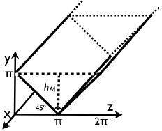
Figure 1: Schematic of straight channel with triangular cross-sections $\Omega=\beta_{45}(z)$ and coordinate system

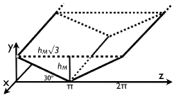
Figure 2: Schematic of straight channel with triangular cross-sections $\Omega=\beta_{30}(z)$ and coordinate system

We consider solutions of the following two forms:

A.

$$\phi(x,y,z,t)=\psi(y,z)\cos(\omega t),$$ (27)

referred to as transverse modes see packham1980small , groves1994hamiltonian .

B.

$$\phi(x,y,z,t)=\psi(y,z)\cos(\kappa x-\omega t),$$ (28)

referred to as longitudinal modes, see packham1980small , kuznetsov2002linear .

We formulate the problem of finding solutions of the above form in terms of Dirichlet-Neumann operators.

We first consider transverse modes. Let the fluid domain consist of a straight channel and consider the case $\Omega=\Omega_{B}.$ Consider $f:[0,b]\rightarrow\mathbb{R}$, and define the Dirichlet-Neumann operator $G_{0}$ by

$$(G_{0}f)(z)=\frac{\partial\psi(z,y)}{\partial y}|_{y=h_{M}},$$ (29)

where $\psi:\Omega\rightarrow\mathbb{R}$ satisfies

$$\left\{\begin{array}[]{l}\Delta\psi=0\text{ }\text{ in }\Omega,\\ \psi=f\text{ at }\Omega\cap\Gamma_{F},\\ \frac{\partial\psi}{\partial{\hat{n}}}=0\text{ }\text{ at }\Omega\cap(\Gamma_{B}\cup\Gamma_{L}),\\ \end{array}\right.$$ (30)

Combining the first two equations of (26), the problem of finding transverse mode solutions (27) can be written as

$$G_{0}f=g^{-1}\omega^{2}f.$$ (31)

The classical (exact) approach to solving (25)-(27), or (29)-(31), is given in subsection 4.1. We will compare the results to solutions of (31) with $G_{0}$ replaced by the operators $\mathcal{A}_{1}(\beta)$, $\mathcal{A}_{G_{0}}(\beta)$, with depth topography as in (21), applied to $b-$periodic functions. We comment on this approximation at the end of this section.

We now consider longitudinal modes. Consider $f(z)=\psi(0,z)$, with $z\in[0,b],$ and define the modified Dirichlet-Neumann operator $G_{0,\kappa}$ by

$$(G_{0,\kappa}f)(z)=\frac{\partial\psi(z,y)}{\partial y}|_{y=h_{M}},$$ (32)

where $\psi:\Omega\rightarrow\mathbb{R}$ satisfies

$$\left\{\begin{array}[]{l}\Delta\psi=\kappa^{2}\psi\text{ }\text{ in }\Omega,\\ \psi=f\text{ at }\Omega\cap\Gamma_{F},\\ \frac{\partial\psi}{\partial{\hat{n}}}=0\text{ }\text{ at }\Omega\cap(\Gamma_{B}\cup\Gamma_{L}),\\ \end{array}\right.$$ (33)

with $\kappa$ as in (28). By (25) and the first two equations of (26), the problem of finding longitudinal mode solutions (28) can be written as

$$G_{0,\kappa}f=g^{-1}\omega^{2}f.$$ (34)

Comparing (25), (28), and the first equation of (33), $(G_{0,\kappa}f)(z)$ in (34) is the 3-D zeroth-order Dirichlet-Neumann operator, $G_{0}$ applied to functions $f(z)e^{\pm i\kappa x}$ (or $f(z)\cos(\kappa x))$.

The classical (exact) approach to solving (25)-(26) and (28), or (32)-(34), is given in subsection 4.2. The solutions will be compared to solutions of (34) with $G_{0,\kappa}$ replaced by operators $\mathcal{A}_{1}$ of (19), $\mathcal{A}_{G_{0}}$ of (20), applied to functions of the form $e^{\pm i\kappa x}f(z)$, with $f$ $b-$periodic. The depth topography is as in (21), and $\beta$ is independent of $x$. Specifically, the operator $\mathcal{A}_{1}$ of (19) applied on functions of the form $e^{\pm i\kappa x}f(z)$ defines the operator $\mathcal{A}_{1,\kappa}(\beta)$ by

$$\mathcal{A}_{1,\kappa}(\beta)f = [\sqrt{D^{2}+\kappa^{2}}\tanh(h_{0}\sqrt{D^{2}+\kappa^{2}})$$

$$-\sqrt{D^{2}+\kappa^{2}}\text{sech}(h_{0}\sqrt{D^{2}+\kappa^{2}})\beta(z)\sqrt{D^{2}+\kappa^{2}}\text{sech}(h_{0}\sqrt{D^{2}+\kappa^{2}})]f,$$

with $h(z)=h_{0}-\beta(z)$, $h_{0}=h_{M}-h_{m}>0$, and $D=-i\partial_{z}$. We will compute numerically the eigenmodes of $\mathcal{A}_{1,\kappa}(\beta)$ with $b-$periodic boundary conditions. Similarly, the ad-hoc operator $\mathcal{A}_{G_{0}}$ of (20) applied on functions of the form $e^{\pm i\kappa x}f(z)$ defines the operator $\mathcal{A}_{G_{0,\kappa}}(\beta)$ by

$$\mathcal{A}_{G_{0,\kappa}}(\beta)f=[\textit{Sym}(\sqrt{D^{2}+\kappa^{2}}\tanh(h(z)\sqrt{D^{2}+\kappa^{2}}))]f,\text{ }\text{}$$ (36)

with the notation of (3), and we will compute the eigenmodes of $\mathcal{A}_{G_{0,\kappa}}(\beta)$ with $b-$periodic boundary conditions. Symmetrization of operators on $b-$periodic functions is as in Section 2, using the standard inner product on real $b-$periodic $L^{2}$ functions.

Computations with $b-$periodic boundary conditions use the periodic analogues of the operators of Section 2 and above. In particular for $a$ a real function and $h$, $r$ real $b-$periodic functions, we let

$$[a(h(z)D)f](z)=\sum\limits_{\lambda=-\infty}^{\infty}a(h(z)\lambda)\hat{f}_{\lambda}e^{i\lambda\frac{2\pi}{b}z},$$ (37)

$$\hat{f}_{\lambda}=\frac{1}{b}\int_{-{\frac{b}{2}}}^{\frac{b}{2}}f(z)e^{-i\lambda\frac{2\pi}{b}z}dz.$$ (38)

Numerical computations use Galerkin truncations of the above operators to modes $|l|\leq l_{max}$. We can simplify the calculations by noting that operators $\mathcal{A}_{1}$, $D\tanh(h(\cdot)D)$, $\mathcal{A}_{2}$ of Section 2 (with ) and $\mathcal{A}_{1,\kappa}(\beta)$, $\mathcal{A}_{G_{0,\kappa}}(\beta)$ above map real-valued functions to real-valued functions, and for $\beta$, $h$ even they also preserve parity, see Appendix A. We can thus consider finite dimensional truncations of expansions in cosines and sines for the even and odd subspaces respectively. The corresponding matrices are block-diagonal. In the case of $D\tanh(h(\cdot)D)$, we compute the matrix for $\textit{Sym}(D\tanh(h(\cdot)D))$ by symmetrizing the truncation of $D\tanh(h(\cdot)D)$. Clearly, the adjoint (transpose) and symmetrization also preserve parity.

In the next section we describe some known semi-analytic solutions of the form (27), (28), obtained for some special domains with finite cross-section $\Omega$ and $\Gamma_{L}=\emptyset$, i.e. slopping beach geometries. These solutions are constructed starting with a multiparameter family of harmonic functions $\phi_{\mu}$ of the form (27), or (28), defined on the plane and satisfying the rigid wall boundary condition on a set ${\tilde{\Gamma}}_{B}$ that includes $\Gamma_{B}$ and is the boundary of a domain $\tilde{\mathcal{D}}$ that includes $\mathcal{D}$. Then we require that the $\phi_{\mu}$ also satisfy the first two equations of (26) on the free surface $\Gamma_{F}$. This requirement leads to algebraic equations that restrict the allowed values of the parameter $\mu$ to a discrete set and also determine the frequencies. This construction does not assume any boundary conditions for the free surface potential.

The second computation in the next section computes $b-$periodic eigenfunctions of the approximate Dirichlet-Neumann operators defined in Section 2 and above, with $b-$periodic depth profiles with vanishing depth at integer multiples of $z=b$. Also, the domains we consider in the next section are symmetric in $z$ so that the eigenfunctions of the approximate Dirichlet-Neumann operators are either even or odd, satisfying Neumann and Dirichlet boundary conditions respectively at $z=0$, $b$.

4 Transverse and longitudinal modes in triangular cross-sections

Transverse and longitudinal modes can be calculated explicitly only for special geometries of the channel cross-sections. In this section we compare some exact results for triangular channels by Lamb lamb1932hydrodynamics Art. 261, Macdonald macdonald1893waves , Greenhill greenhill1887wave , Packham packham1980small , and Groves groves1994hamiltonian , to results obtained using the approximate Dirichlet-Neumann operators defined in the previous sections.

4.1 Transverse modes for triangular cross-section: right isosceles triangle

The first geometry we consider corresponds to a uniform straight channel with right isosceles triangle as a cross-section, see Figure 3. The cross-section $\Omega=\Omega_{B}$ is as in (21) and the bottom is at $y=\beta_{45}(z)$. The minimum and maximum heights of the the fluid domain are $h_{m}=0$ and $h_{M}=\pi$ respectively The channel width is $b=2\pi$, and

$$\beta_{45}(z)=\left\{\begin{array}[]{l}-z+\pi\text{ }\text{ in }0\leq z<\pi\\ z-\pi\text{ }\text{ in }\pi\leq z\leq 2\pi.\\ \end{array}\right.$$ (39)

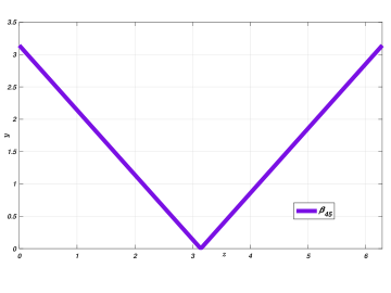
Figure 3: Right isosceles triangular cross-section of a straight channel with the right angle at the bottom, see equation (39)

Normal modes for this channel were obtained by Kirchhoff, see Lamb lamb1932hydrodynamics , Art. 261, and include symmetric and antisymmetric modes. The symmetric transverse modes, see (27), are given by potentials $\phi(x,y,z,t)=\psi(y,z)\cos(\omega t)$ with

$$\psi(y,z)=A[\cosh(\alpha z)\cos(\beta y)+\cos(\beta z)\cosh(\alpha y)].$$ (40)

It can be checked that $\frac{\partial\phi}{\partial y}\mid_{y=h_{M}}$ and $\phi$ are symmetric with respect to the $z=0$ axis. Also, $\phi$ in harmonic in the quarter plane $y\geq|z|$, and satisfies the rigid wall boundary condition

$$\frac{\partial\phi}{\partial\hat{n}}=0\quad\text{at}\quad y=|z|.$$ (41)

To impose the boundary condition at the free surface $y=h_{M}$, we use the first two equations of (26) to obtain

$$\omega^{2}\psi=g\frac{\partial\psi}{\partial y}\quad\text{at}\quad y=h_{M}.$$ (42)

Combining with (40) we have the conditions

$$\alpha^{2}-\beta^{2}=0,$$ (43)

and

$$\omega^{2}\cosh(\alpha h_{M})=g\alpha\sinh(\alpha h_{M}),\quad\omega^{2}\cos(\beta h_{M})=-g\beta\sin(\beta h_{M})=0,$$ (44)

or equivalently

$$\alpha h_{M}\tanh(\alpha h_{M})+\beta h_{M}\tan(\beta h_{M})=0.$$ (45)

The values of $\alpha$, $\beta$ are determined by the intersections of the curves (43) and (45), see Figure 4. There is an infinite number of solutions, $h_{M}\alpha_{j}$, $j=0,2,4,\ldots$, with $\alpha_{j}<\alpha_{j^{\prime}}$ if $j<j^{\prime}$. The corresponding frequencies $\omega_{j}$ are obtained by (44). The first values of $h_{M}\alpha_{i},\omega_{i}$ are shown in Table 1.

To obtain the antisymmetric modes we use the potentials $\phi(x,y,z,t)=\psi(y,z)\cos(\omega t)$ with

$$\psi(y,z)=B[\sinh(\alpha z)\sin(\beta y)+\sin(\beta z)\sinh(\alpha y)].$$ (46)

We check that $\phi$ satisfies the rigid wall boundary conditions at $y=|z|$ and is harmonic in the quadrant $y\geq|z|$. We also check that $\frac{\partial\phi}{\partial y}\mid_{y=h_{M}}$ is antisymmetric with respect to the $z=0$ axis. Imposing the free surface boundary conditions (26) to (27) we obtain (42). Then (46) leads to the conditions

$$\alpha^{2}-\beta^{2}=0$$ (47)

and

$$\omega^{2}\sinh(\alpha h_{M})=g\alpha\cosh(\alpha h_{M}),\quad\omega^{2}\sin(\beta h_{M})=g\beta\cos(\beta h_{M}),$$ (48)

or

$$\alpha h\coth(\alpha h_{M})=\beta h_{M}\cot(\beta h_{M}).$$ (49)

The values of $\alpha$, $\beta$ are determined by the intersections of the curves (47) and (49), see Figure 5. There is an infinite number of solutions $h_{M}\alpha_{j}$, $j={1,3,5...}$ with $\alpha_{j}<\alpha_{j^{\prime}}$ if $j<j^{\prime}$. The corresponding frequencies $\omega_{j}$ are given by (48), see Table 1.

By the first two equations of (26), and the form of $\phi$, the free surface corresponding to the above symmetric and antisymmetric satisfies

$$\eta(x,z,t)=-\frac{1}{g}\omega\psi(y,z)\mid_{y=h_{M}}\sin\omega t=\frac{1}{\omega}\frac{\partial\psi(y,z)}{\partial y}\mid_{y=h_{M}}\sin\omega t.$$ (50)

The amplitude of $\eta$ is therefore $\omega^{-1}\frac{\partial\psi(y,z)}{\partial y}\mid_{y=h_{M}}$.

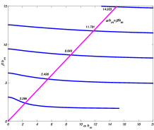
Figure 4: Even modes. Intersection of curves (43) and (45)

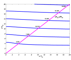
Figure 5: Odd modes. Intersection of curves (47) and (49)

Table 1: Frequencies of modes for channel of Figure 3 these values are associated to graphic roots in Figure 4 and 5 We use $h_{M}=\pi$

	$i=0$	$i=1$	$i=2$	$i=3$	$i=4$	$i=5$	$\cdots$
$\alpha_{i}h_{M}$	2.365	3.927	5.498	10.210	11.781	16.494	$\cdots$
$\omega_{i}$	4.8624	7.8261	4.1413	5.6445	6.0622	7.1684	$\cdots$

In Figure 6 we compare the surface amplitude of the exact symmetric and antisymmetric modes found above to the surface amplitudes obtained by computing numerically the eigenfunctions of the approximate Dirichlet-Neumann operators ${\mathcal{A}}_{G_{0}}(\beta_{45^{\circ}})$ of (15), and $\mathcal{A}_{1}(\beta_{45^{\circ}})$ with $2\pi-$periodic boundary conditions. The surface amplitude $\eta$ is obtained by $\eta=\omega^{-1}\mathcal{A}(\beta)f$, with ${\mathcal{A}}(\beta)$ representing each of the two approximate Dirichlet-Neumann operators. This expression is analogous to (50).

Figure 6 suggests good quantitative agreement between the exact even modes and the even modes obtained by $\mathcal{A}_{G_{0}}$, $\mathcal{A}_{1}(\beta)$, with some discrepancy near the boundary for the first mode. The $\mathcal{A}_{G_{0}}$ modes seem closer to the exact ones in the interior. For the odd modes, the two approximate operators lead to vanishing amplitude at the boundary. This is a consequence of the parity considerations of the previous section. On the other hand, exact odd modes have non-vanishing values at the boundary, in fact they appear to have local extrema at the boundary. This leads to a discrepancy between exact and approximate modes at the boundary. The first two modes of $\mathcal{A}_{G_{0}}$, $\mathcal{A}_{1}(\beta)$ and of the exact approach differ quite significantly also in the interior of the domain, with the $\mathcal{A}_{G_{0}}$ modes being somewhat closer to the exact ones. For higher modes, the discrepancy at the boundary persists, but the values of the interior are close for all four sets of modes.

The procedure for obtaining the exact modes does not require any conditions on the value of the potential at the intersection of the free boundary and the rigid wall. Also, the free surface is described by a value of the $y-$coordinate, and this allows us to define $\eta(z)$ for all real $z$, in particular we determine the fluid domain by computing the intersection of the graph of $\eta$ with the rigid wall (Figure 6 only shows $\eta(z)$, $z\in[0,2\pi]$). The exact approach leads then to a more realistic motion of the surface at the sloping beach. This does not imply that the exact solutions are physical either, since the boundary conditions at the free surface are not exact. In contrast, the odd modes of the approximate operators correspond to pinned boundary conditions that are not expected to be physical.

We have also used the operators $\mathcal{A}_{G_{0}}(\beta_{30^{\circ}})$ and $\mathcal{A}_{1}(\beta_{30^{\circ}})$ to compute the $2\pi-$periodic normal modes of domains obtained from the triangular channel by adding an interval of extra depth, see Figure 7. We denote the added depth by $T$. Figure 8 indicate the convergence as $T$ vanishes of the modes obtained for $\mathcal{A}_{G_{0}}(\beta_{45})$ for $T>0$ to the corresponding modes obtained for the triangular domain $T=0$. Similar results were obtained for the other operators. Also, even modes satisfy a Neumann boundary condition at $z=0$, $2\pi$, and the interval of length $T$ can be interpreted also as the height of a vertical wall at $z=0$, $2\pi$.

Convergence to the triangular domain modes indicates more clearly that normal modes of the approximate, $2\pi-$periodic operators used for a triangular domain are limiting cases of operators defined for a $2\pi-$periodic depth profile, with depth that does not vanish anywhere. In that case the definition and computations of the Dirichlet-Neumann operator follow the construction of CGNS , but can not take into account the sloping beach boundary. Note also that the $2\pi-$periodic modes obtained using the $2\pi-$periodic $\mathcal{A}_{G_{0}}(\beta_{30^{\circ}})$, $\mathcal{A}_{1}(\beta_{30^{\circ}})$, are special cases of the Floquet-Bloch modes for the $2\pi-$periodic depth profile see arXiv:1706.07417 submitted manuscript by W. Craig, M. Gazeau, C. Lacave, C. Sulem. for a study of the the band structure and Floquet-Bloch modes of $\mathcal{A}_{1}(\beta)$ with another periodic profile.

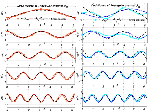
Figure 6: Transverse modes of a channel with isosceles triangular cross-section illustrated in Figure 3. Left: Even modes. Orange (circle-line): operator $\mathcal{A}_{1}(\beta_{45^{\circ}})$.Red (dot-dashed-line): operator $\mathcal{A}_{G_{0}}(\beta_{45^{\circ}})$. Black dashed lines: exact solutions given by (40) and the values in Table 1. Right: Odd modes. Cian (circle-line): operator $\mathcal{A}_{1}(\beta_{45^{\circ}})$. Blue (dot-dashed-line): operator $\mathcal{A}_{G_{0}}(\beta_{45^{\circ}})$. exact solutions given by (46) and the values in Table 1

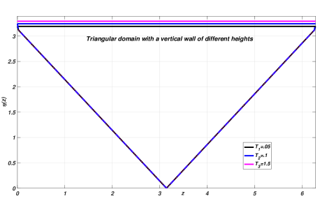
Figure 7: Cross section of the straight channels with lateral boundary $\Gamma_{L}$. Vertical walls of heights $T_{1}=0.05$ (black), $T_{2}=0.1$ (red), $T_{3}=.15$ (blue)

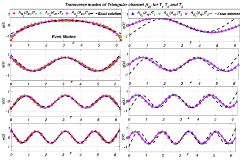
Figure 8: Transverse modes with $\mathcal{A}_{G_{0}}(\beta_{45})$ for the three cross sections of Figure 7, vertical segments of heights $T_{1}=.006$ (red), $T_{2}=.15$ (green) , $T_{3}=.6$ (magenta)

4.2 Longitudinal modes for triangular cross-sections: isosceles triangle with unequal angle of $120^{\circ}$

A second geometry with exact longitudinal modes was considered by Macdonald macdonald1893waves , Packham, packham1980small , see also Lamb lamb1932hydrodynamics , Art. 261. This geometry corresponds to a uniform straight channel with isosceles triangle cross-section with a unequal angle at the bottom of $120^{\circ}$, as illustrated in Figure 9. In this case we will examine longitudinal modes.

We consider the cross-section $\Omega=\Omega_{B}$, as in (21) and the bottom $\beta_{30^{\circ}}(z)$ of (51). The channel width is $b=2\pi$ and the maximum and minimum heights of the fluid domain are $h_{M}=\frac{\pi}{\sqrt{3}}$ and $h_{m}=0$ respectively. The cross-section profile is given by

$$\beta_{30^{\circ}}(z)=\left\{\begin{array}[]{l}\frac{-1}{\sqrt{3}}z+\frac{\pi}{\sqrt{3}},0\leq z<\pi\\ \frac{1}{\sqrt{3}}z-\frac{\pi}{\sqrt{3}},\pi\leq z\leq 2\pi\\ \end{array}\right.,z\in[0,2\pi].$$ (51)

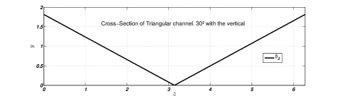
Figure 9: Straight channel with isosceles triangular cross-section with the unequal angle at the bottom of $120^{\circ}$ , see equation (51)

The exact solutions for symmetric modes, see Packham packham1980small , and Groves groves1994hamiltonian are as follows.

The $0-$mode is described by a velocity potential $\phi$ of the form (28) with

$$\psi(z,y) = A[\cosh(\kappa(y-h_{M}))+\frac{\omega^{2}\kappa^{2}}{g\kappa}\sinh(\kappa(y-h_{M}))$$

$$+2\cosh(\frac{\sqrt{3}\kappa(z-\pi)}{2})$$

$$\times\{\cosh(\kappa(\frac{y}{2}+h_{M}))-\frac{\omega^{2}\kappa^{2}}{g\kappa}\sinh(\kappa(\frac{y}{2}+h_{M}))\}],$$

and

$$\omega^{2}=\frac{3g}{4\kappa}\coth(\frac{3\kappa h_{M}}{2})\{1+(1-\frac{8}{9}\tanh^{2}(\frac{3\kappa h_{M}}{2}))^{\frac{1}{2}}\}.$$ (53)

The remaining symmetric modes $2,4,6,8,...$ are described by a velocity potential $\phi$ of the form (28) with

$$\psi(y,z) = A[\{\cosh(\alpha(y-h_{M}))+\frac{\omega^{2}\kappa^{2}}{g\kappa}\sinh(\alpha(y-h_{M}))\}\cos(\beta(z-\pi))$$

$$+2\cosh(\frac{\sqrt{3}\alpha(z-\pi)}{2})\cos(\frac{\sqrt{3}\beta y}{2})\cos(\frac{\beta(z-\pi)}{2})$$

$$\times\{\cosh(\alpha(\frac{y}{2}+h_{M}))-\frac{\omega^{2}\kappa^{2}}{g\kappa}\sinh(\alpha(\frac{y}{2}+h_{M}))\}$$

$$-2\sinh(\frac{\sqrt{3}\alpha(z-\pi)}{2})\sin(\frac{\sqrt{3}\beta y}{2}\sin(\frac{\beta(z-\pi)}{2}))$$

$$\times\{\sinh(\alpha(\frac{y}{2}+h_{M}))-\frac{\omega^{2}\kappa^{2}}{g\kappa}\cosh(\alpha(\frac{y}{2}+h_{M}))\}],$$

and

$$\omega^{2}=\frac{g\alpha}{\kappa^{2}}\left[\frac{\frac{\beta}{\alpha}\sqrt{3}(\cosh(3\alpha h_{M})-\cos(\sqrt{3}\beta h_{M}))}{\frac{\beta}{\alpha}\sqrt{3}\sinh(3\alpha h_{M})-3\sin(\sqrt{3}\beta h_{M})}\right].$$ (55)

The above potentials are harmonic and satisfy the rigid wall boundary conditions.

The first two equations of motion of (26), (28), and (4.2) lead to

$$\alpha^{2}-\beta^{2}=\kappa^{2},$$ (56)

and

$$\left(\frac{\beta}{\alpha}\right)^{2}\cosh(3\alpha h_{M})\cos(\sqrt{3}\beta h_{M})$$

$$- \frac{1}{4}\left(\frac{\beta}{\alpha}\right)\sqrt{3}\left\{1-\left(\frac{\beta}{\alpha}\right)^{2}\right\}\sinh(3\alpha h_{M})\sin(\sqrt{3}\beta h_{M})$$

$$-\frac{1}{4}\left[\left\{3+5\left(\frac{\beta}{\alpha}\right)^{2}\right\}-\left\{3+\left(\frac{\beta}{\alpha}\right)^{2}\right\}\cos^{2}(\sqrt{3}\beta h_{M})\right]=0.$$

In Figure 11 we show the symmetric longitudinal modes derived with the values of $\alpha$ and $\beta$ obtained from relations (56) and (4.2) for $\kappa=2$, see also Table 2.

By the first two equations of (26) and (28), the free surface corresponding to the above modes can be computed by

$$\eta(z,t)=-\frac{1}{\omega}\frac{\partial\psi(y,z)}{\partial y}\mid_{y=h_{M}}\sin\omega t.$$ (58)

The amplitude of $\eta$ is therefore $\omega^{-1}\frac{\partial\psi(y,z)}{\partial y}\mid_{y=h_{M}}$.

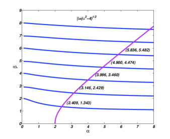
Figure 10: Graphs for the determination of $\alpha$ and $\beta$ for the modes $2$, $4$, $6$, $8$, and $10$ using $\kappa=2$, $h_{M}=\frac{\pi}{\sqrt{3}}$

Table 2: Frequencies of modes of channel of Figure 9 these values are associated to graphic roots in Figure 10. We use $h_{M}=\frac{\pi}{\sqrt{3}}$

	$i=2$	$i=4$	$i=6$	$i=8$	$i=10$	$\cdots$
$\alpha_{i}$	2.409	3.146	3.996	4.900	5.836	$\cdots$
$\beta_{i}$	1.343	2.429	3.460	4.474	5.482	$\cdots$
$\omega_{i}$	2.4297	2.7764	3.1289	3.4651	3.7813	$\cdots$

In Figure 11 we compare the surface amplitude of the exact symmetric modes to the surface amplitudes obtained by computing numerically the eigenfunctions of the approximate Dirichlet-Neumann operators $\mathcal{A}_{G_{0,\kappa}}(\beta)$, $\mathcal{A}_{1,\kappa}(\beta)$ of (36), (3) respectively, with $\beta$ as in (51). We use $\kappa=2$. To compute the eigenfunctions of ${\mathcal{A}}_{G_{0,\kappa}}(\beta)$, $\mathcal{A}_{1,\kappa}(\beta)$ numerically we use $2\pi-$periodic boundary conditions. Also, given a computed eigenfunction $f$ of ${\mathcal{A}}={\mathcal{A}}_{G_{0,\kappa}}(\beta)$ or $\mathcal{A}_{1,\kappa}(\beta)$ the surface amplitude $\eta$ is given by $\eta=\omega^{-1}\mathcal{A}$. This is analogous to (58).

By Figure 11 we see some discrepancies between the first exact even mode and the first even ${\mathcal{A}}_{G_{0,\kappa}}(\beta)$ mode. For higher even modes, the ${\mathcal{A}}_{G_{0,\kappa}}(\beta)$ modes are close to the exact modes in the interior, but show discrepancies at the boundary. Also the even modes obtained by ${\mathcal{A}}_{G_{0,\kappa}}(\beta)$, $\mathcal{A}_{1,\kappa}(\beta)$ are generally close both in the interior and the boundary, with more pronounced discrepancies for the first and second modes.

To our knowledge there are no exact solutions reported in the literature for odd modes. Odd modes obtained with the approximate Dirichlet-Neumann operators $\mathcal{A}_{G_{0,\kappa}}(\beta_{30^{\circ}})$, $\mathcal{A}_{1,\kappa}(\beta_{30^{\circ}})$ are shown in Figure 11.

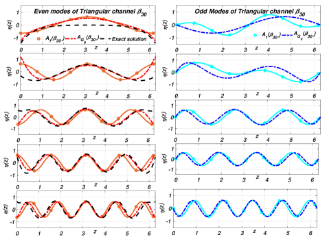
Figure 11: Longitudinal modes of a channel with isosceles triangular cross-section illustrated in Figure LABEL:Figtrian30. Left: Even modes with $\kappa=2$. Orange(circle-line): operator $\mathcal{A}_{1}(\beta_{30^{\circ}})$. Red (dot-dashed-line): operator $\mathcal{A}_{G_{0}}(\beta_{30^{\circ}})$. Black dashed lines: exact solutions given by (4.2) and (55) and the values in Table 2. Right: Odd modes with $\kappa=2$. Cian (circle-line): operator $\mathcal{A}_{1}(\beta_{30^{\circ}})$ with $\kappa=2$. Blue (dot-dashed-line): operator $\mathcal{A}_{G_{0}}(\beta_{30^{\circ}})$.

5 Discussion

We have studied linear water wave modes in channels with variable depth, choosing depth geometries and models with known exact results. The main goal was to test simplifications of the lowest order variable depth Dirichlet-Neumann operator for variable depth. The exact results involve slopping beach geometries, while the approximate Dirichlet-Neumann operators we use are seen to be limits of approximate Dirichlet-Neumann operators for periodic topographies with nowhere vanishing depth. This observation suggests that the problems we compare are not equivalent. Despite this fact we see reasonable agreement in the interior of the domain, with most discrepancies at the boundary of the free surface.

In the case of 2-D even modes the approximate operators yield good approximations of the exact modes even at the boundary. In the case of 2-D odd modes, the approximate Dirichlet-Neumann operators impose Dirichlet boundary conditions and miss the boundary behavior of the exact modes. In general, the exact modes seem to have local extrema at the boundary, and this may explain why the even modes of the periodic approximate Dirichlet-Neumann operators may give a better fit. We also think that Neumann boundary conditions, allowing odd modes, may give better approximations. In the case of 3-D longitudinal waves, the exact approach only yields even modes. The approximate operators give reasonable approximations of the exact modes in the interior of the domain, but can miss the boundary behavior. We suspect that Neumann boundary conditions may also be more appropriate.

Appendix A

We present some computations related to symmetrization, parity, and the operator $D\tanh(h(\cdot)D)$.

The notion of adjoint $\mathcal{A}^{*}$ applies to operators $\mathcal{A}:D(\mathcal{A})\subset L^{2}\rightarrow L^{2}$, with $D(\mathcal{A})$ dense in $L^{2}=L^{2}(\mathbb{R};\mathbb{R})$. Operators that map real-valued functions to real-valued (resp. imaginary-valued) functions will be denoted as real (resp. imaginary) operators. Imaginary operators map $D(\mathcal{A})\subset L^{2}$ to $iL^{2}$. The adjoint and symmetrization of a real operator is real. We extend the definition of the adjoint to imaginary operators linearity by requiring $\langle\mathcal{A}f,g\rangle=\langle f,\mathcal{A}^{*}g\rangle$, for all $f\in D(\mathcal{A})$. Letting $\mathcal{B}=i\mathcal{A}$, we have $\mathcal{A}^{*}=-i\mathcal{B}^{*}$. We note that $D$ and $\tanh(h(x)D)f$ are imaginary, and therefore $D\tanh(h(x)D)f$ is real. Similarly, we check that operators $\mathcal{A}_{1}$, $\mathcal{A}_{2}$, $\mathcal{A}_{1,\kappa}(\beta)$, $\mathcal{A}_{G_{0,\kappa}}(\beta)$ are also real.

Also, for $\beta$, $h$ even we check that $\mathcal{A}_{1}$, $\mathcal{A}_{2}$, $D\tanh(h(x)D)$, $\mathcal{A}_{1,\kappa}(\beta)$, and $\mathcal{A}_{G_{0,\kappa}}(\beta)$ preserve parity, i.e. map even (resp. odd) real-valued functions to even (resp. odd) real-valued functions. This follows by examining the various operators appearing in the respective definitions and their compositions.

For instance, the operator $D$ maps even (resp. odd) real-valued functions to odd (resp. even) imaginary-valued functions. Also, by the definition of $\tanh(h(x)D)$ on the line,

$$g_{1}(x) = \tanh(h(x)D)\cos kx=\frac{1}{2}[\tanh(h(x)k)e^{ikx}+\tanh(h(x)(-k)e^{-ikx}]$$

$$= i\tanh(h(x)k)\sin kx,$$

$$g_{2}(x) = \tanh(h(x)D)\sin kx=\frac{1}{2i}[\tanh(h(x)k)e^{ikx}-\tanh(h(x)(-k))e^{-ikx}]$$

$$= -i\tanh(h(x)k)\cos kx.$$

Then $h$ even implies $g_{1}(-x)=-g_{1}(x)$, and $g_{2}(-x)=g_{2}(x)$, for all $x$. Therefore $\tanh(h(x)D)$ maps even (resp. odd) real-valued functions to odd (resp. even) imaginary-valued functions, and $D\tanh(h(x)D)$ is real and preserves parity Similar calculations apply to $b-$periodic functions, e.g. with $k$ integer if $b=2\pi$. Operators $\mathcal{A}_{1,\kappa}(\beta)$ of (3) and $\mathcal{A}_{G_{0,\kappa}}(\beta)$ of (36) are compositions of real operators that preserve parity.

We now consider the operator $\mathcal{A}_{G_{0}}$ up to order one in $\beta$. We have

$$[D\tanh(h(x)D)f](x) = -i\partial_{x}(2\pi)^{-1}\int_{\mathbb{R}}\tanh(h(x)k)\hat{f}(k)e^{ikx}dk$$ (59)

$$= (2\pi)^{-1}[-i\int_{\mathbb{R}}[(\partial_{x}\tanh(h(x)k))\hat{f}(k)e^{ikx}dk$$

$$\qquad\qquad\qquad\qquad+\int_{\mathbb{R}}(\tanh(h(x)k))\hat{f}(k)ke^{ikx}dk]$$

$$= (2\pi)^{-1}[i\beta^{\prime}(x)\int_{\mathbb{R}}\text{sech}^{2}(h(x)k)k\hat{f}(k)e^{ikx}dk$$

$$\qquad\qquad\qquad\qquad+\int_{\mathbb{R}}(\tanh(h(x)k))\hat{f}(k)ke^{ikx}dk]$$

$$= i\beta^{\prime}(x)[\text{sech}^{2}(h(x)D)Df](x)+[\tanh(h(x)D)Df](x),$$

using

$$\partial_{x}(\tanh(h(x)k)) = \partial_{x}(\tanh(h(x)k)\partial_{x}(h(x)k)$$

$$= \partial_{x}(\tanh(h(x)k))h^{\prime}(x)k$$

$$= -\text{sech}^{2}(h(x)k)\beta^{\prime}(x)k,$$

and $\partial_{x}h(x)=\partial_{x}(h_{0}-\beta(x))=-\beta^{\prime}(x)$. Furthermore

$$[i\beta^{\prime}(x)\text{sech}^{2}(h(x)D)Df](x) = i\beta^{\prime}(x)(2\pi)^{-1}\int_{\mathbb{R}}[\text{sech}^{2}(h_{0}k)+O(\beta^{2})]k\hat{f}(k)e^{ikx}dk$$

$$= i\beta^{\prime}(x)[\text{sech}^{2}(h_{0}D)D^{2}f](x)+O(\beta^{2}),$$

and

$$[\tanh(h(x)D)Df](x) = \int_{\mathbb{R}}\left(\tanh(h_{0}k)-\text{sech}^{2}(h_{0}k)\beta(x)k+O(\beta^{2})\right)\hat{f}(k)ke^{ikx}\frac{dk}{2\pi}$$

$$= [\tanh(h_{0}D)Df](x)-\beta(x)[\text{sech}^{2}(h_{0}D)D^{2}f](x)+O(\beta^{2}).$$

Therefore (59) leads to

$$D\tanh(h(x)D) = \tanh(h_{0}D)D+i\beta^{\prime}\text{sech}^{2}(h_{0}D)D-\beta\text{sech}^{2}(h_{0}D)D^{2}+O(\beta^{2}).$$

We also have $(\tanh(h_{0}D))^{*}=-\tanh(h_{0}D)$, $D^{*}=-D$, $(\text{sech}^{2}(h_{0}D))^{*}=\text{sech}^{2}(h_{0}D)$, $(i\beta\cdot)^{*}=i\beta\cdot$, $(\beta\cdot)^{*}=\beta\cdot$, so that

$$\textit{Sym}(D\tanh(h(x)D)) = D\tanh(h_{0}D)+\frac{1}{2}[i\beta^{\prime}\text{sech}^{2}(h_{0}D)D-\beta\text{sech}^{2}(h_{0}D)D^{2}$$ (60)

$$-iD\text{sech}^{2}(h_{0}D)\beta^{\prime}+D^{2}\text{sech}^{2}(h_{0}D)\beta]+O(\beta^{2}).$$

Operators $\text{sech}^{2}(h_{0}D)$, $\beta\cdot$ (with $\beta$ even) are real and preserve parity, while $i\beta^{\prime}\cdot$, and $D$ are imaginary and reverse parity. It follows that the operator $\mathcal{A}_{2}$ of (2) obtained by truncating (60) to $O(\beta^{2})$ is real and preserves parity.

References

- (1) Aceves-Sánchez P., Minzoni A. A., Panayotaros P.: Numerical study of a nonlocal model for water-waves with variable depth. Wave Motion, 50(1), 80- 93 (2013)
- (2) Andrade D., Nachbin A.: A three-dimensional Dirichlet-to-Neumann operator for water waves over topography. J. Fluid Mech., 845, 321-345 (2018)
- (3) J. D. Carter: Bidirectional Whitham equations as models of waves in shallow water. Wave Motion 82, 51-62 (2018)
- (4) Constantin A., Escher J.: Wave breaking for nonlinear nonlocal shallow water equations. Acta Mathematica, 181(2), 229-243 (1998)
- (5) Craig W., Groves M. D.: Hamiltonian long-wave approximations to the water-wave problem. Wave Motion, 19(4), 367-389 (1994)
- (6) Craig W., Guyenne P., Nicholls D.P., Sulem C.: Hamiltonian long-wave expansions for water waves over a rough bottom. In Proc. Royal Soc. London A: Math., Phys. Eng. Sci.,46, 839-873 (2005)
- (7) Craig W., Sulem C.: Numerical simulation of gravity waves. J. Comp. Phys., 108(1), 73-83, (1993)
- (8) Ehrnström M., Kalisch H.: Traveling waves for the Whitham equation. Diff. Int. Eq., 22(11/12), 1193-1210 (2009)
- (9) Ehrnström M., Groves M.D., Wahlénn E.: On the existence and stability of solitary-wave solutions to a class of evolution equations of whitham type. Nonlinearity, 25(10), 2903 (2012)
- (10) Evans D. V., Linton C.M.: Sloshing frequencies. Quart. J. Mech. Appl. Math. 46(1), 71-87 (1993)
- (11) A. G. Greenhill. Wave motion in hydrodynamics (continued). Amer. J. Math., 97-112 (1887)
- (12) Groves M.D.: Hamiltonian long-wave theory for water waves in a channel. Quart. J. Mech. Appl. Math., 47, 367-404 (1994)
- (13) Gouin M., Ducrozet G., Ferrant P.: Development and validation of a highly nonlinear model for wave propagation over a variable bathymetry. In ASME 2015 34th International Conference on Ocean, Offshore and Arctic Engineering, pages V007T06A077-V007T06A077. American Society of Mechanical Engineers, (2015)
- (14) Hur V., Tao L.: Wave breaking in shallow water model. SIAM J. Math. Anal. 50, 354-380 (2018)
- (15) Hur, V. M. : Wave breaking in the Whitham equation. Advances in Mathematics, 317, 410-437 (2017)
- (16) Kuznetsov N., Maz’ya V., Vainberg B.: Linear water waves: a mathematical approach. Cambridge University Press, Cambridge (2002)
- (17) H. Lamb H.: Hydrodynamics. Cambridge University Press, Cambridge (1932)
- (18) Lannes D.: The water wave problem. Mathematical Surveys and Monographs, AMS, 188, (2013)
- (19) Macdonald H.M.: Waves in canals. Proc. London Math. Soc., 1(1), 101-113 (1893)
- (20) Miles J. W.: On Hamilton’s principle for surface waves. J. Fluid Mech., 83(01),153-158 (1977)
- (21) D. Moldabayev, H. Kalisch, and D. Dutykh: The Whitham Equation as a model for surface water waves. The Whitham Equation as a model for surface water waves. Physica D: Nonlinear Phenomena, 309, 99-107 (2015)
- (22) Naumkin P. I., Shishmarev J. A.: Nonlinear nonlocal equations in the theory of waves. A.M.S., (1994)
- (23) Packham B. A.: Small-amplitude waves in a straight channel of uniform triangular cross-section. Quart. Jour. Mech. Appl. Math., 33(2), 179-187 (1980)
- (24) Radder A. C.: An explicit Hamiltonian formulation of surface waves in water of finite depth. J. Fluid Mech., 237, 435-455 (1992)
- (25) Vargas-Magaña R. M, Panayotaros P.: A Whitham-Boussinesq long-wave model for variable topography. Wave Motion, 65, 156-174 (2016)
- (26) Whitham G. B.: Linear and nonlinear waves. John Wiley & Sons, 42 (2011)
- (27) Zakharov V.E.: Stability of periodic waves of finite amplitude on the surface of a deep fluid. J. Appl. Mech. Tech. Phys., 9(2), 190-194 (1968)