Anti-de-Sitter-Maxwell-Yang-Mills black holes thermodynamics from nonlocal observables point of view

Abstract

In this paper we analyze the thermodynamic properties of the Anti de Sitter black hole in the Einstein-Maxwell-Yang-Mills-AdS gravity (EMYM) via many approaches and in different thermodynamical ensembles (canonical/ grand canonical). First, we give a concise overview of this phase structure in the entropy-thermal diagram for fixed charges then we investigate this thermodynamical structure in fixed potentials ensemble. The Next relevant step is recalling the nonlocal observables such as holographic entanglement entropy and two-point correlation function to show that both observables exhibit a Van der Waals-like behavior in our numerical accuracy and just near the critical line as the case of the thermal entropy for fixed charges by checking Maxwell’s equal area law and the critical exponent.

In the light of the grand canonical ensemble, we also find a newly phase structure for such a black hole where the critical behavior disappears in the thermal picture as well as in the holographic one.

1 Introduction

Over the last years, a great emphasis has been put on the application of the Anti-de-Sitter/Conformal field theory correspondence [1, 2] which plays a pivotal role in recent developments of many physical themes[3, 4, 5], in this particular context the thermodynamic of anti-de-Sitter black holes become more attractive for investigation [6].

In general, black hole thermodynamics has emerged as a fascinating laboratory for testing the predictions of candidate theories of quantum gravity. It has been figured that black holes are associated thermodynamically with a entropy and a temperature[7] and a pressure[8]. This association has led to a rich structure of phase picture and a remarkable critical behavior similar to van der Waals liquid/gas phase transition. [9, 10, 11, 12, 13, 14, 15, 16, 17, 18, 19, 20, 21, 22, 23, 24, 25]. Another confirmation of this similarity appear when we employ non-local observables such as entanglement entropy, Wilson loop, two point correlation function and the complexity growth rate [31, 32, 33, 26, 27, 28, 29, 30, 34, 39, 35, 36, 37, 38]. Meanwhile, these tools are used extensively in quantum information and to characterize phases and thermodynamical behavior [40, 41, 42, 43, 44, 45, 46, 47, 48, 49].

The black hole charge finds a deep interpretation in the context of the AdS/CFT correspondence linked to condensed matter physics, the charged black hole introduces a charge density/chemical potential and temperature in the quantum field theory defined on the boundary [50]. In this background, the charged black hole can be viewed as un uncondensed unstable phase which develops a scalar hair at low temperature and breaks $U(1)$ symmetry near the black hole horizon reminiscing the second order phase transition between conductor and superconductor phases [51], this situation is called the ”s-wave” holographic superconductor. It has also been shown that ”p-wave” holographic superconductor corresponds to vector hair models [52, 53]. The simplest example of p-wave holographic superconductors may be provided by an Einstein-Yang-Mills theory with $SU(2)$ gauge group and no scalar fields, where the electromagnetic gauge symmetry is identified with an $U(1)$ subgroup of $SU(2)$. The other components of the $SU(2)$ gauge field play the role of charged fields dual to some vector operators whose break the $U(1)$ symmetry, leading to a phase transition in the dual field theory.

Motived by all the ideas described above, although the Yang-Mills fields are confined to acting inside nuclei while the Maxwell field dominates outside, the consideration of such theory where the two kinds of field live is encouraged by the existence of exotic and highly dense matter in our universe. In this work, we try to contribute to this rich area by revisiting the phase transition of Anti-de-Sitter black holes in Einstein-Maxwell-Yang-Mills (EMYM) gravity. More especially, we investigate the first and second order phase transition by different approaches including the holographic one and in different canonical ensembles.

This work is organized as follow: First, we present some thermodynamic properties and phase structure of the EMYM-AdS black holes in (Temperature, entropy)-plane in canonical and grand canonical ensemble. Next, we show in section 3 that the holographic approach exhibit the same behavior, in other words we recall the entanglement entropy and two-point correlation function to check the Maxwell’s equal area law and calculating the critical exponent of the specific heat capacity which is consistent with that of the mean field theory of the Van der Waals in the canonical ensemble near the critical point. In the grand canonical one, a new phase structure arise where the critical behavior disappears in the thermal as well as the holographic framework. The last section is devoted to a conclusion.

2 Critical behavior of Einstein-Maxwell-Yang-Mills-AdS black holes in thermal picture

2.1 Canonical ensemble

We start this section by writing the $N$-dimensional for Einstein-Maxwell-Yang-Mills gravity with a cosmological constant $\Lambda$ described by the following action [54, 55]

$${\cal I}=\frac{1}{2}\int_{\mathcal{M}}dx^{N}\sqrt{-g}\left(R-\frac{(N-1)(N-2)}{3}\Lambda-\mathcal{F}_{M}-\mathcal{F}_{YM}\right),$$ (1)

where $R$ is the Ricci scalar while $\Lambda$ is the cosmological constant. Also $\mathcal{F}_{M}=F_{\mu\nu}F^{\mu\nu}$ and $\mathcal{F}_{YM}=\textbf{Tr}(F^{(a)}_{\mu\nu}F^{(a)\mu\nu})$ are the Maxwell invariant and the Yang-Mills invariant respectively, the trace element stands for $\textbf{Tr}(.)=\sum_{a=1}^{(N-1)(N-2)/2}(.)$. Varying the action (1) with respect to the metric tensor $g_{\mu\nu}$, the Faraday tensor $F_{\mu\nu}$, and the YM tensor $F^{(a)}_{\mu\nu}$, one can obtain the following field equations

$$G_{\mu\nu}+\Lambda g_{\mu\nu}=T^{M}_{\mu\nu}+T^{YM}_{\mu\nu}$$ (2)

$$\nabla F^{\mu\nu}=0$$ (3)

$$\hat{D}_{\mu}F^{(a)}_{\mu\nu}=\nabla_{\mu}F^{(a)\ \mu\nu}+\frac{1}{\Theta}\varepsilon^{(a)}_{(b)(c)}A^{(b)}_{\mu}F^{(c)\ \mu\nu}=0$$ (4)

where $G_{\mu\nu}$ is the Einstein tensor, the quantity $\varepsilon^{(a)}_{(b)(c)}$’s stands for the structure constants of the $\frac{(N-1)(N-2)}{2}$-parameters Lie group $G$, $\Theta$ is coupling constant and $A^{(a)}_{\mu}$ denote the $SO(N-1)$ gauge groupe YM potential. We also note that the internal indices $\{a,b,c,...\}$ do not differ whether in covariant or contravariant form. In addition, $T^{M}_{\mu\nu}$ and T${}^{YM}_{\mu\nu}$ are the energy momentum tensor of Maxwell and YM fields with the following formula

$$T^{M}_{\mu\nu} = -\frac{1}{2}g_{\mu\nu}F_{\rho\sigma}F^{\rho\sigma}+2F_{\mu\lambda}F^{\lambda}_{\nu}$$ (5)

$$T^{YM}_{\mu\nu} = \sum_{a=1}^{(N-1)(N-2)/2}\left[-\frac{1}{2}g_{\mu\nu}F^{(a)}_{\rho\sigma}F^{(a)\rho\sigma}+2F^{(a)}_{\mu\lambda}F^{(a)\lambda}_{\nu}\right]$$ (6)

$$F_{\mu\nu}^{(a)}=\partial_{\mu}A_{\nu}^{(a)}-\partial_{\nu}A_{\mu}^{(a)}+\frac{1}{2\Theta}\varepsilon_{(b)(c)}^{(a)}A_{\mu}^{b}A_{\nu}^{c},$$ (7)

$$F_{\mu\nu}=\partial_{\mu}A_{\nu}-\partial_{\nu}A_{\mu}.$$ (8)

Where $A_{\mu}$ is the usual Maxwell potential. The metric for such $N$ dimensional spherical black hole may be chosen to be [55]

$$ds^{2}=-f(r)dt^{2}+\frac{1}{f(r)}dr^{2}+r^{2}d\Omega_{n}^{2}$$ (9)

in which, $d\Omega_{n}^{2}$ represents the volume of the unit $n$-sphere which can be expressed in the standard spherical form

$$d\Omega_{N-2}^{2}=d\theta_{1}^{2}+\sum_{i=2}^{N-3}\Pi_{j=1}^{i-1}\sin^{2}\theta_{j}\;d\theta_{i}^{2}\ \ \text{ where }\ \ \ \ 0\leq\theta_{1}\leq\pi,0\leq\theta_{i}\leq 2\pi.$$ (10)

In order to find the electromagnetic field, we recall the following radial gauge potential ansatz $A_{\mu}=h(r)\delta_{\mu}^{0}$ which obeys to the Maxwell field equations (3) with the following solution

$$\frac{dh(r)}{dr}=\frac{c}{r^{N-2}}$$ (11)

where $c$ is an integration constant related to electric charge $C$ of the solutions. To solve the YM field, Eq.(4), we use the magnetic Wu–Yang ansatz of the gauge potential [56, 57] given by

$$A^{(a)} = \frac{Q}{r^{2}}\left(x_{i}dx_{j}-x_{j}dx_{i}\right)$$ (12)

$$2 \leq i\leq N-1,$$

$$1 \leq j\leq i-1$$

$$1 \leq \left(a\right)\leq\left(N-1\right)(N-2)/2$$

where we imply (to have a systematic process) that the super indices $a$ is chosen according to the values of $i$ and $j$ in order. For instance, we present some of them

$$\begin{array}[]{c}A^{\left(1\right)}=\frac{Q}{r^{2}}\left(x_{2}dx_{1}-x_{1}dx_{2}\right)\\ A^{\left(2\right)}=\frac{Q}{r^{2}}\left(x_{3}dx_{1}-x_{1}dx_{3}\right)\\ A^{\left(3\right)}=\frac{Q}{r^{2}}\left(x_{3}dx_{2}-x_{2}dx_{3}\right)\\ A^{\left(4\right)}=\frac{Q}{r^{2}}\left(x_{4}dx_{1}-x_{1}dx_{4}\right)\\ A^{\left(5\right)}=\frac{Q}{r^{2}}\left(x_{4}dx_{2}-x_{2}dx_{4}\right)\\ A^{\left(6\right)}=\frac{Q}{r^{2}}\left(x_{4}dx_{3}-x_{3}dx_{4}\right)\\ A^{\left(7\right)}=\frac{Q}{r^{2}}\left(x_{5}dx_{1}-x_{1}dx_{5}\right)\\ A^{\left(8\right)}=\frac{Q}{r^{2}}\left(x_{5}dx_{2}-x_{2}dx_{5}\right)\\ A^{\left(9\right)}=\frac{Q}{r^{2}}\left(x_{5}dx_{3}-x_{3}dx_{5}\right)\\ A^{\left(10\right)}=\frac{Q}{r^{2}}\left(x_{5}dx_{4}-x_{4}dx_{5}\right)\\ ...\end{array}$$ (13)

in which $r^{2}=\overset{N-1}{\underset{i=1}{\sum}}x_{i}^{2}.$ The YM field 2-forms are defined by the expression

$$F^{\left(a\right)}=dA^{\left(a\right)}+\frac{1}{2Q}\varepsilon_{\left(b\right)\left(c\right)}^{\left(a\right)}A^{\left(b\right)}\wedge A^{\left(c\right)}.$$ (14)

In general for $N$ we must have $\left(N-1\right)\left(N-2\right)/2$ gauge potentials. The integrability conditions

$$dF^{\left(a\right)}+\frac{1}{Q}\varepsilon_{\left(b\right)\left(c\right)}^{\left(a\right)}A^{\left(b\right)}\wedge F^{\left(c\right)}=0$$ (15)

are easily satisfied by using (28). The YM equations

$$d\ast F^{\left(a\right)}+\frac{1}{Q}\varepsilon_{\left(b\right)\left(c\right)}^{\left(a\right)}A^{\left(b\right)}\wedge\ast F^{\left(c\right)}=0$$ (16)

also are all satisfied. The energy-momentum tensor (4), becomes after

$$\sum_{a=1}^{\left(N-1\right)\left(N-2\right)/2}\left[F_{\lambda\sigma}^{\left(a\right)}F^{\left(a\right)\lambda\sigma}\right]=\frac{\left(N-3\right)\left(N-2\right)Q^{2}}{r^{4}}$$ (17)

with the non-zero components

$$T_{00} = \frac{\left(N-3\right)\left(N-2\right)Q^{2}f\left(r\right)}{2r^{4}}$$ (18)

$$T_{11} = -\frac{\left(N-3\right)\left(N-2\right)Q^{2}}{2r^{4}f\left(r\right)}$$

$$T_{22} = -\frac{\left(N-3\right)\left(N-6\right)Q^{2}}{2r^{2}}$$

$$T_{AA} = -\frac{\left(N-3\right)\left(N-6\right)Q^{2}}{2r^{2}}\Pi_{i=1}^{A-2}\sin^{2}\theta_{i}$$

$$2 < A\leq N-1.$$

Using the Eq.(2) and after some simplifications, one can find that the metric function $f(r)$ has the following form is given by

$$f(r) = 1-\frac{2m}{r^{n-1}}-\frac{\Lambda}{3}r^{2}+\frac{2(n-1)C^{2}}{nr^{2n-2}}-\frac{(n-1)Q^{2}}{(n-3)r^{2}},$$ (19)

Where $N=n+2$, one can note in the particular case for $n=3$ the last term of Eq.(19) diverges, involving an unusual logarithmic term in Yang-Mills charge [54]. For this gravity background the parameter $m$ is related to the mass of such black hole, while $C$ and $Q$ are the charges of Maxwell field and Yang-Mills field respectively. Following previous literature [8, 9], one can finds a close connection between the cosmological constant and pressure as $P=-\frac{\Lambda}{8\pi}$, leading to the following expressions of Hawking temperature, mass and entropy of such black hole in term of the horizon radius $r_{+}$

$$T=\frac{f^{\prime}(r_{+})}{4\pi}=\frac{n-1}{4\pi r_{+}}+\frac{2(n+1)P}{3}r_{+}-\frac{(n-1)Q^{2}}{4\pi r^{3}}-\frac{(n-1)^{2}C^{2}}{2\pi nr_{+}^{2n-1}},$$ (20)

$$M=\frac{n\omega_{n}}{48\pi}\big{(}8\pi Pr_{+}^{n+1}+\frac{3(n-1)Q^{2}r^{n-3}}{3-n}+3r_{+}^{n-1}+\frac{6(n-1)C^{2}}{nr_{+}^{n-1}}\big{)},$$ (21)

$$S=\frac{\omega_{n}r_{+}^{n}}{4},$$ (22)

The Yang-Mills potential $\Phi_{Q}$ and the electromagnetic one $\Phi_{C}$ can be written as

$$\Phi_{Q}=\left(\frac{\partial M}{\partial Q}\right)_{C,P,r_{+}}=\frac{\omega_{n}(n-1)nQ}{8\pi(3-n)}r_{+}^{n-3},$$ (23)

$$\Phi_{C}=\left(\frac{\partial M}{\partial C}\right)_{Q,P,r_{+}}=\frac{\omega_{n}(n-1)C}{4\pi r_{+}^{n-1}},$$ (24)

where $\omega_{n}=\frac{2\pi^{(n+1)/2}}{\Gamma(\frac{n+1}{2})}$ is the volume of the unit $n$-sphere. In fact, according to the interpretation of the black hole mass $M$ as an enthalpy [8] in the extended phase space context, the free energy $\mathcal{F}$ of black hole can be written as

$$\mathcal{F}=M-T\cdot S$$ (25)

and the heat capacity is given by

$$C_{Q}=\left.T\frac{\partial S}{\partial T}\right|_{Q}$$ (26)

It straightforward to show that obtained quantities Eq.(20), Eq.(21) and Eq.(22), obey to the first law of black hole thermodynamics in the extended phase space

$$dM=TdS+\Phi_{Q}dQ+\Phi_{C}dC+VdP,$$ (27)

where $V$ is the Legendre transform of the pressure, which denotes the thermodynamic volume with

$$V=\left(\frac{\partial M}{\partial P}\right)_{S,\Phi_{Q},\Phi_{C}}=\frac{n\omega_{n}\pi}{3}r^{n+1}.$$ (28)

In addition to this, using scaling argument, the corresponding Smarr formula is

$$M=\frac{n}{n-1}TS+\Phi_{C}C+\frac{1}{(n-1)}\Phi_{Q}Q-\frac{2}{n-1}VP.$$ (29)

Without loss of generality, inserting Eq.(22) into Eq.(20), we can get the entropy Hawking temperature relation of such black hole, namely

$$T = \frac{1}{12\pi n}\left[6C(n-1)^{2}\left(4^{\frac{1}{n}}\left(\frac{S}{\omega_{n}}\right)^{\frac{1}{n}}\right)^{1-2n}+\pi 2^{\frac{2}{n}+3}n(n+1)P\left(\frac{S}{\omega_{n}}\right)^{\frac{1}{n}}-3(n-1)nQ^{2}4^{\frac{-3}{n}}\left(\frac{S}{\omega_{n}}\right)^{\frac{-3}{n}}\right.$$ (30)

$$+ \left.3\ 4^{-1/n}(n-1)n\left(\frac{S}{\omega_{n}}\right)^{-1/n}\right]$$

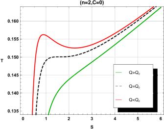
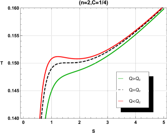
Figure 1: The temperature as a function of the entropy for different values of charge $C$. (Left) $C=0$. (Right) $C\neq 0$.

This relation is depicted in Fig.1, indeed it has been shown that there is a Van der Waals-like phase transition, furthermore a direct confirmation comes from the solution of the following system

$$\left(\frac{\partial T}{\partial S}\right)_{Q}=\left(\frac{\partial^{2}T}{\partial S^{2}}\right)_{Q}=0.$$ (31)

which reveal the existence of a critical point. The critical charge, entropy, and temperature are given in the following Tab.1 with for all the rest of the paper we keep $n=2$.

	$Q_{c}$	$S_{c}$	$T_{c}$
${\tt C=0}$	$\frac{1}{2\sqrt{3}}$	$\frac{\pi}{2}$	$\frac{\sqrt{2}}{3\pi}$
${\tt C\neq 0}$	$\frac{1}{6}\sqrt{3-36C^{2}}$	$\frac{\pi}{2}$	$\frac{\sqrt{2}}{3\pi}$

Table 1: Coordinates of the critical points for different values of $C$ in $(T,S)$-diagram.

An important remark can be observed here is that both quantities $T_{c}$ and $S_{c}$ are insensible the charge $C$. The behavior of the free energy $\mathcal{F}$ with respect to the temperature may be investigated by plotting in the Fig.2 the graph $\mathcal{F}-T$ for a fixed value of charge $Q$ under the critical one. From this plot, we can observe the characteristic swallow-tail which guarantees the existence of the Van der Waals-like phase transition.

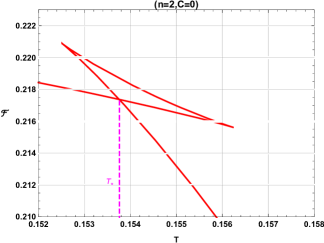
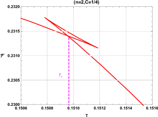
Figure 2: The Helmholtz free energy in function of the entropy for EMYM-AdS black holes for different values of the charge $C$. (Left) $C=0$. (Right) $C\neq 0$.

Using the Fig.2, we can derive numerically the coexistence temperature $T_{\star}$ needed in the Maxwell’s equal area law construction

$$A_{1}\equiv\int_{S_{1}}^{S_{2}}T(S)dS-T_{\star}(S_{2}-S_{1})=T_{\star}(S_{3}-S_{2})-\int_{S_{2}}^{S_{3}}T(S)dS\equiv A_{2},$$ (32)

where $S_{3}$, $S_{2}$ and $S_{1}$ are the solutions of $T(S)=T_{\star}$ in descending order, in addition to the numerical values of these point and the we report in in Tab.2 the area $A_{1}$ and $A_{2}$ in Maxwell’s law Eq.(32)

C	$T_{\star}$	$S_{1}$	$S_{2}$	$S_{3}$	$A_{1}$	$A_{2}$
${\tt 0}$	0.15376	0.638237	1.52994	3.13241	0.383499	0.38350
${\tt\frac{1}{4}}$	150965	1.05043	11.54616	2.25932	00.18248	0.1825

Table 2: Check of the equal area law in the $T-S$ plane for different $C$.

Obviously, the area $A_{1}$ equals to area $A_{2}$ for different $C$, so the equal area law doesn’t break. For the second phase transition, we know that near the critical point, there is always a linear relation with slope equal to $3$ [55, 58]

$$log|T-T_{c}|=3\ log|S-S_{c}|+constant$$ (33)

in this context, the heat capacity behaves like

$$C_{Q}\sim(T-T_{c})^{-2/3}$$ (34)

where the critical exponent of the second order phase is $-2/3$, which is consistent with the mean field theory.

2.2 Grand canonical ensemble

Having described the thermodynamical behavior of the EMYM-AdS black hole with a fixed charge, by showing the occurrence of the first and second phase transition, we will focus on this section to the phase structure when the potentials are kept fix.

To facilitate the calculation of relevant quantities, it is convenient to reexpress the Hawking temperature as a function of entropy, Yang-Mills and electromagnetic potentials, inserting Eq.23 and Eq.(24) into Eq.(30) on can write

$$T = \frac{1}{3\pi 2^{\frac{2(n+1)}{n}}}\left(\frac{S}{\omega_{n}}\right)^{-1/n}$$

$$\times \left[\frac{96\pi^{2}\left(-\frac{2^{\frac{n+8}{n}}(n-3)^{2}\Phi_{Q}^{2}\left(4^{\frac{1}{n}}\left(\frac{S}{\omega_{n}}\right)^{\frac{1}{n}}\right)^{-2n}\left(\frac{S}{\omega_{n}}\right)^{4/n}}{n-1}-n\Phi_{c}^{2}\right)}{n^{2}\omega_{n}^{2}}-16^{\frac{1}{n}}\Lambda(n+1)\left(\frac{S}{\omega_{n}}\right)^{2/n}+3(n-1)\right]$$

In our assumptions, where $n=2$ and $\Lambda=-1$, the Eq.(2.2) reduces to

$$T=\frac{S-\pi\left(\Phi_{c}^{2}+\Phi_{Q}^{2}-1\right)}{4\pi^{3/2}\sqrt{S}}$$ (36)

which is in agreement with the result of [59, 60] if we set $\Phi_{Q}=0$. Now we are able to write easily

$$\left(\frac{\partial T}{\partial S}\right)_{\Phi_{Q},\Phi_{c}}=\frac{-S-3\pi\left(\Phi_{c}^{2}+\Phi_{Q}^{2}-1\right)}{16\pi^{3/2}S^{5/2}}$$ (37)

$$\left(\frac{\partial^{2}T}{\partial S^{2}}\right)_{\Phi_{Q},\Phi_{c}}=\frac{S+\pi\left(\Phi_{c}^{2}+\Phi_{Q}^{2}-1\right)}{8\pi^{3/2}S^{3/2}}$$ (38)

The solution of the $\left(\frac{\partial T}{\partial S}\right)_{\Phi_{Q},\Phi_{c}}=0$ can be derived as

$$S_{1}=-\pi\left(\Phi_{c}^{2}+\Phi_{Q}^{2}-1\right)$$ (39)

with the condition $\Phi_{c}^{2}+\Phi_{Q}^{2}<1$ should be verified to ensure that the entropy in Eq.(39) is positive. In the other case $\Phi_{c}^{2}+\Phi_{Q}^{2}>1$, one can’t find meaningful root of the equation $\left(\frac{\partial T}{\partial S}\right)_{\Phi_{Q},\Phi_{c}}=0$. Substituting Eq.(39) into Eq.(38) we obtain the following constraint

$$\left.\left(\frac{\partial^{2}T}{\partial S^{2}}\right)_{\Phi_{Q},\Phi_{c}}\right|_{S=S_{1}}=\frac{1}{8\pi^{3}\left(-\Phi_{c}^{2}-\Phi_{Q}^{2}+1\right)^{3/2}}>0$$ (40)

implying that, no critical point is observed in the $T-S$ diagram. This observation differs from the result in the previous section where the charges are kept fixed, consolidating the assertion that the thermodynamics in the grand canonical ensemble is quite different from that in the canonical one. In Fig.3, we depict the Hawking temperature for both the case $\Phi_{c}^{2}+\Phi_{Q}^{2}<1$ and $\Phi_{c}^{2}+\Phi_{Q}^{2}>1$ and one can see that there exists minimum temperature for the left panel . Substituting Eq.(39) into Eq.(36), the minimum temperature can be obtained as

$$T_{min}=\frac{\sqrt{-\Phi_{c}^{2}-\Phi_{Q}^{2}+1}}{2\pi}.$$ (41)

While, the Hawking temperature increases monotonically in the right panel.

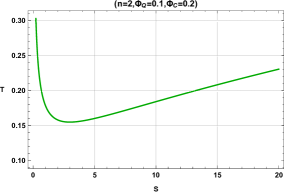
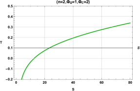
Figure 3: The temperature as a function of the entropy for different potentials. (Left) $\Phi_{c}^{2}+\Phi_{Q}^{2}<1$. (Right) $\Phi_{c}^{2}+\Phi_{Q}^{2}>1$.

Having obtained the phase picture of the thermal entropy of the AdS-Maxwell-Yang-Mills black hole the canonical/grand canonical ensemble, we will now revisit the phase structure of the entanglement entropy and two-point correlation function to see whether they have similar phase structure in each thermodynamical ensemble.

3 Phase transitions of Einstein-Maxwell-Yang-Mills-AdS black holes in holographic picture

3.1 Holographic entanglement entropy

First, let us provide a concise review of some generalities about the holographic entanglement entropy. For a given quantum field theory described by a density matrix $\rho$, with $A$ is some region of a Cauchy surface of spacetime and $A^{c}$ stands for its complement, the von Neumann entropy which traduce the entanglement between these two regions

$$S_{A}=-\mathrm{Tr}_{A}{(\rho_{A}\log{\rho_{A}})}\,,$$ (42)

with $\rho_{A}$ is the reduced density matrix of given by $A$ $\rho_{A}=\mathrm{Tr}_{A^{c}}{(\rho)}$. Ryu and Takayanagi propose a simple geometric way to evaluate the entanglement entropy as [61, 62]

$$S_{A}=\frac{\text{Area}(\Gamma_{A})}{4G_{N}}\,,$$ (43)

in which $\Gamma_{A}$ denote a codimension-2 minimal surface with boundary condition $\partial\Gamma_{A}=\partial A$, and $G_{N}$ stands for the gravitational Newton’s constant. In our black hole model we choose the region $A$ to be a spherical cap on the boundary delimited by $\theta\leq\theta_{0}$, and the minimal surface can be parametrized by the function $r{(\theta)}$. According to definition of the area and Eq.(9) and Eq.(43) on can show that the holographic entanglement entropy is governed by

$$S_{A}=\frac{\omega_{n-2}}{4}\int_{0}^{\theta_{0}}r^{n-2}\sin^{n-2}{\theta}\sqrt{\frac{(r^{\prime})^{2}}{f{(r)}}+r^{2}}d\theta\,,$$ (44)

where the notation prime denotes the derivative with respect to $\theta$ e.g. $r^{\prime}\equiv\frac{dr}{d\theta}$. Treating the Eq.(44) as a Lagrangian and solving the equation of motion given by

$$r^{\prime}(\theta)^{2}[\sin\theta r(\theta)^{2}f^{\prime}(r)-2\cos\theta r^{\prime}(\theta)]-2r(\theta)f(r)[r(\theta)(\sin\theta r^{\prime\prime}(\theta)+\cos\theta r^{\prime}(\theta))-3\sin\theta r^{\prime}(\theta)^{2}]$$ (45)

$$+ 4\sin(\theta)r(\theta)^{3}f(r)^{2}=0.$$

Due to the difficulty to find an analytical form of the solution $r{(\theta)}$, we will perform a numerical calculation with adopting the following boundary conditions

$$r^{\prime}(\theta)=0,\;\;r(0)=r_{0}.$$ (46)

Knowing that the entanglement entropy is divergent at the boundary, we regularized it by subtracting the area of the minimal surface in pure AdS whose boundary is also $\theta=\theta_{0}$ with

$$r_{AdS}{(\theta)}=L\left(\left(\frac{\cos{\theta}}{\cos{\theta_{0}}}\right)^{2}-1\right)^{-1/2}\,.$$ (47)

We label the regularized entanglement entropy by $\Delta S_{A}$ and for our numerical calculation we choose $\theta_{0}=0.2$, and $0.3$ while Ultra Violet cutoff is chosen to be $\theta_{c}=0.199$ and $0.299$ respectively. To compare with the phase structure in the thermal picture, we will study the relation between the entanglement entropy and the Hawking temperature representing the temperature of the dual field theory, this relation is depicted in Fig.4 for different values of Maxwell’s charge with a fixed Yang-Mills one near the critical point and the chosen $\theta_{0}$.

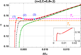
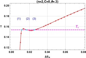
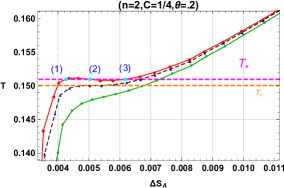
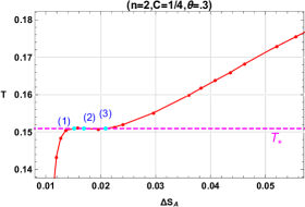
Figure 4: Plot of isocharges on the $(T,\Delta S_{A})$-plan, for different values of $\theta_{0},\;C$. For all panels: the values of the charge are $Q=.9Q_{c}$ (red), $Q=Q_{c}$ (dashed black) and $Q=2Q_{c}$ (green). The coexistence phase isotherm $T_{\star}$ (dashed magenta line) is obtained from the free energy Figure.2 and the critical temperature (dashed orange line). For all curves, we also show the data points which are used to create the interpolation.

For each panel, the red lines are associated with a charge less than the critical one while equal to the critical charge are depicted in black dashed lines and green lines correspond to a charge upper than the critical. Especially, the first order phase transition temperature $T_{\star}$ and second-order phase transition temperature $T_{c}$ are plotted by magenta and orange dashed line respectively. As can be seen in all these plots, the Van der Waals-like phase structure can also be observed in the $T-\Delta S_{A}$diagram. Particularly, the coexistence temperature $T_{\star}$ and second-order phase transition temperature $T_{c}$ are exactly the same as that in the thermal entropy structure.

Adopting the same steps as in the thermal picture, we will also check numerically whether Maxwell’s equal area law holds

$$A_{1}=\int_{\Delta S_{A}^{(1)}}^{\Delta S_{A}^{(2)}}T{(\Delta S_{A},Q)}d\Delta S_{A}-T_{*}(\Delta S_{A}^{(2)}-\Delta S_{A}^{(1)})$$ (48)

$$A_{2}=T_{*}(\Delta S_{A}^{(3)}-\Delta S_{A}^{(2)})-\int_{\Delta S_{A}^{(2)}}^{\Delta S_{A}^{(3)}}T{(\Delta S_{A},Q)}d\Delta S_{A}$$ (49)

with the quantities $\Delta S_{A}^{(1)}$, $\Delta S_{A}^{(2)}$ and $\Delta S_{A}^{(3)}$ are roots of the equation $T_{*}=T{(\Delta S_{A},Q)}$ in the ascending order. The Maxwell’s equal area law stipulate that

$$A_{1}=A_{2}.$$ (50)

We tabulate in Tab.3 the values of the both areas $A_{1}$ and $A_{2}$ for the chosen $\theta_{0}$, the charge $C$ as well as the relative error between $A_{1}$ and $A_{2}$ taken to be the difference between $A_{1}$ and $A_{2}$ divided by their average.

$C$	$\frac{Q}{Q_{c}}$	$\theta_{0}$	$\Delta S_{A}^{(1)}$	$\Delta S_{A}^{(2)}$	$\Delta S_{A}^{(3)}$	$A_{1}$	$A_{2}$	Relative error
$0$	0.9	0.2	$0.00339417$	$0.00490769$	$0.00755095$	$2.271\times 10^{-6}$	$2.218\times 10^{-6}$	2.36 %
		0.3	$0.011477$	$0.0164978$	$0.0254236$	$6.563\times 10^{-6}$	$6.407\times 10^{-6}$	$2.4\%$
	0.5	0.2	$0.00161291$	$0.0042458$	$0.0130777$	$0.00007432$	$0.00005560$	$28.81\%$
$\frac{1}{4}$	0.9	0.2	$0.00425941$	$0.00502275$	$0.00617356$	$9.961\times 10^{-8}$	$1.023\times 10^{-7}$	$2.66\%$
		0.3	$0.0151665$	$0.0169359$	$0.0208834$	$1.601\times 10^{-7}$	$1.631\times 10^{-7}$	$1.85\%$
	0.5	0.2	$0.00339968$	$0.00496717$	$0.00743883$	$2.12718\times 10^{-6}$	$1.76781\times 10^{-6}$	$18.44\%$

Table 3: Comparison of $A_{1}$ and $A_{2}$ for the EMPYM-AdS black hole using entanglement entropy.

Based on Tab.3, we can see that, as the pressure approaches the critical one, the relative error which translates the disagreement between Maxwell’s areas decreases. We can claim that the first order phase transition of the holographic entanglement entropy obeys to Maxwell’s equal area law just near the critical point and within our numerical accuracy.

The next obvious step in our investigation is the check of the critical exponent of the second order phase transition by analyzing the slope of the relation between $log|T-T_{c}|$ and $log|\Delta S_{A}-\Delta S_{A_{c}}|$, where $\Delta S_{A_{c}}$ is the critical entanglement entropy found numerically by an equation $T(\Delta S_{A})=T_{c}$ . We also introduce the definition of an analog to heat capacity by writing

$$\mathcal{C}_{Q}=\left.T\frac{\partial(\Delta S_{A})}{\partial T}\right|_{Q}.$$ (51)

Taking $\theta_{0}=0.2$ and for different charge $C$ , we plot the relationship between $log|T-T_{c}|$ and $log|\Delta S_{A}-\Delta S_{A_{c}}|$ in Fig.5, and the analytical relation can be fitted as

$$log|T-T_{c}|=\left\{\begin{array}[]{cc}14.2558+{\bf 3.09904}\ log|\Delta S_{A}-\Delta S_{A_{c}}|&(C=0)\\ 2.9293+{\bf 3.031061}\ log|\Delta S_{A}-\Delta S_{A_{c}}|&(C=\frac{1}{4})\\ \end{array}\right.$$ (52)

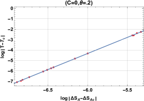
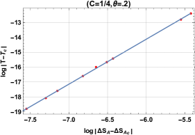
Figure 5: The relation between $log|T-T_{c}|$ and $log|\Delta S_{A}-\Delta S_{A_{c}}|$ for different $C$. (Left) $C=0$. (Right) $C\neq 0$.

The slop of Eq.(52) is around $3$ indicating that the critical exponent is $-2/3$ in total concordance with that in Eq.(33), therefore the critical exponent for second-order phase transition of the holographic entanglement entropy agrees with that of the thermal entropy in the canonical ensemble [55, 58] .

Now, we turn our attention to the grand canonical ensemble, we adopt the same analysis and the chosen values of the previous subsection, by writing the Eq.(19) and Eq.(45) as a function of the potentials $\Phi_{Q}$ and $\Phi_{c}$, taking the same boundary conditions Eq.(46), we perform the numerical calculations used in the plot of Hawking temperature as a function of the holographic entanglement entropy with fixed potentials in Fig.6.

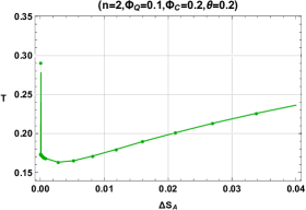
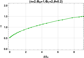
Figure 6: The relation between $log|T-T_{c}|$ and $log|\Delta S_{A}-\Delta S_{A_{c}}|$ for different $C$. (Left) $(\Phi_{c}=0.1,\Phi_{Q}=0.2)$. (Right) $(\Phi_{c}=1,\Phi_{Q}=2)$.

Comparing Fig.3 with Fig.6, one may find that the thermal picture shares the same behavior of the holographic entanglement entropy, we can also observe the same minimum value of the temperature $T_{min}=0.155125$. Then the holographic framework reproduces the same attitude of the $T-S$ diagram in the grand canonical ensemble.

Now, after showing that the holographic entanglement entropy shears the same phase picture as that of the thermal entropy for grand canonical and just near the critical point for the canonical ensemble since the relative disagreement between Maxwell’s areas can become significantly large at low pressure. We attempt in the next section to explore whether the two-point correlation function has the similar behavior as that of the entanglement entropy.

3.2 Two point correlation function

According to the Anti-de-Sitter/Conformal fields theory correspondence, the time two-point correlation function can be written under the saddle-point assumption and in the large limit of $\Delta$ as [63]

$$\langle{\cal{O}}(t_{0},x_{i}){\cal{O}}(t_{0},x_{j})\rangle\approx e^{-\Delta{L}},$$ (53)

where $\Delta$ is the conformal dimension of the scalar operator $\mathcal{O}$ in the dual field theory, the quantity $L$ stands for the length of the bulk geodesic between the points $(t_{0},x_{i})$ and $(t_{0},x_{j})$ on the AdS boundary. Taking into account the symmetry of the considered black hole spacetime, we can simply $x_{i}=\theta$ with the boundary $\theta_{0}$ and employ it to parameterize the trajectory. In this case, the proper length can be expressed as

$$L=\int_{0}^{\theta_{0}}\mathcal{L}(r(\theta),\theta)d\theta,~{}~{}\mathcal{L}=\sqrt{\frac{(r^{\prime}(\theta))^{2}}{f(r(\theta))}+r(\theta)^{2}},\ \ \text{ where }\ \ \ r^{\prime}=dr/d\theta$$ (54)

Treating $\mathcal{L}$ as Lagrangian and $\theta$ as time, one can write the equation of motion for $r(\theta)$ as

$$r^{\prime}(\theta)^{2}f^{\prime}(r(\theta))-2f(r(\theta))r^{\prime\prime}(\theta)+2r(\theta)f(r(\theta))^{2}=0.$$ (55)

Recalling the boundary conditions of Eq.(46) we attempt to solve this equation by choosing the same background of the previous section, in other words the same values of the parameter $\theta_{0}$ with the same UV cutoff values in the dual field theory. The regularized two-point correlation function is labeled as $\Delta L_{A}=L-L_{0}$, where $L_{0}$ denotes the geodesic length in pure AdS under the same boundary region. In Fig.7 we have depicted the behavior of the temperature $T$ in function of $\Delta L_{A}$, the all plots show the Van der Waals-like phase transition as in the case of the thermal and the holographic entanglement entropy portrait.

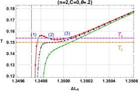
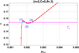
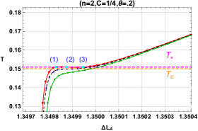
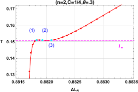
Figure 7: Plot of isocharges on the $(T,\Delta L_{A})$-plan, for $C=0$ (left), and $C\neq 0$ (right). For all panels: the values of the charge are $Q=0.9Q_{c}$ (red), $Q=Q_{c}$ (dashed black) and $Q=2Q_{c}$ (green).

As in the case of the holographic entanglement entropy, the relevant calculated results are listed in Tab.4 which are the $\theta_{0}$ values, the $\Delta\mathcal{L}_{A_{1,2,3}}$ and the areas $A_{1}$, and $A_{2}$.

$C$	$\frac{Q}{Q_{c}}$	$\theta_{0}$	$\Delta L_{A}^{(1)}$	$\Delta L_{A}^{(2)}$	$\Delta L_{A}^{(3)}$	$A_{1}$	$A_{2}$	relative error
$0$	0.9	0.2	$1.34978$	$1.34987$	$1.35003$	$0.000287$	$0.000300$	$4.42\%$
		$0.3$	$0.881705$	$0.881911$	$0.882274$	$0.000197$	$0.000208$	$5.43\%$
	0.4	0.2	$1.34967$	$1.34983$	$1.35043$	$0.001431$	$0.001812$	$23.49\%$
$\frac{1}{4}$	0.9	0.2	$1.34983$	$1.34988$	$1.34995$	$0.000142$	$0.000138$	$2.85\%$
		0.3	$0.881822$	$0.881926$	$0.882085$	$0.000209$	$0.000216$	$3.29\%$
	0.4	0.2	$1.34978$	$1.34987$	$1.35003$	$0.0003907$	$0.0004653$	$17.42\%$

Table 4: Comparison of $A_{1}$ and $A_{2}$ for the EMYM-AdS black hole using two point correlation function.

The results of the Tab.4 tell us that under our numerical accuracy and just near the critical point Maxwell’s equal area law still verified implying $A_{1}$ and $A_{2}$ are equal in the proximity to the critical pressure. These remarks consolidate the behavior of all panels of Fig.7. At this point, one can conclude that like the entanglement entropy, the two-point correlation function also exhibits apparently a first order phase transition as that of the thermal entropy. However, exploring broader ranges of the pressure has revealed the fact that the equal area law does not also hold.

For the second phase transition, we will be interested in the quantities $log|T-T_{c}|$ and $log|\Delta L_{A}-\Delta L_{A_{c}}|$ in which $\Delta L_{A_{c}}$ is the obtained numerically by the equation $T(\Delta L_{A})=T_{c}$. The relations between the logarithm of $|T-T_{c}|$ and $|\Delta L_{A}-\Delta L_{A_{c}}|$ are shown in Fig.8

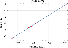
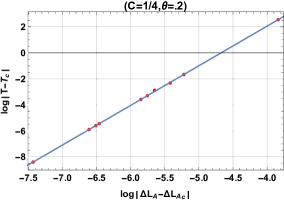
Figure 8: The relation between $log|T-T_{c}|$ and $log|\Delta L_{A}-\Delta L_{A_{c}}|$ for different charge $C$.

The straight blue line in each panel of Fig.8 is fitted following the linear equations

$$log|T-T_{c}|=\left\{\begin{array}[]{cc}19.056+{\bf 3.03594}\ log|\Delta L_{A}-\Delta L_{A_{c}}|&(C=0)\\ 14.25487+{\bf 3.04967}\ log|\Delta L_{A}-\Delta L_{A_{c}}|&(C=\frac{1}{4})\\ \end{array}\right.$$ (56)

Again, we found a slope around 3, then the critical exponent of the specific heat capacity is consistent with that of the mean field theory of the Van der Waals as in the thermal and entanglement entropy portraits [55, 58]. Therefore, we conclude that the two-point correlation function of the Anti-de-Sitter-Maxwell-Yang-Mills black hole exists a second order phase transition at the critical temperature $T_{c}$.

For the grand canonical ensemble, we also plot the temperature $T$ in function of $\Delta L_{A}$ in the Fig.9, from which we can see that thermodynamical behavior is held as the thermal and the holographic entanglement entropy frameworks.

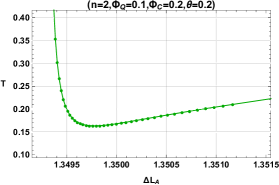
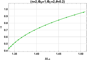
Figure 9: The relation between $log|T-T_{c}|$ and $log|\Delta S_{A}-\Delta S_{A_{c}}|$ for different $C$. (Left) $(\Phi_{c}=0.1,\Phi_{Q}=0.2)$. (Right) $(\Phi_{c}=1,\Phi_{Q}=2)$.

At this level we remark radical rupture appears when we change the thermodynamical ensemble (canonical/grand canonical). The complete comprehension of such different behaviors is not yet completely understood. We believe that it’s typical of such system [49].

4 Conclusion

In this work We have investigated the phase transition of Anti-de-Sitter black hole in the Einstein-Maxwell-Yang-Mills gravity with considering the canonical and the grand canonical ensemble. We first studied the phase structure of the thermal entropy in the $(T,S)$- plane for fixed charges and found that the phase structure agrees with the study made in [55] when the electrodynamics is linear. The authors consider the thermodynamics of such black hole in the $(P,V)$-plane notably the critical behavior and the analogy with the Van der Waals gas. We also have shown that this behavior disappears in the grand canonical ensemble where the potentials $\Phi_{Q}$ and $\Phi_{c}$ are kept fixed.

After, we found that this phase structure of the EMYM-AdS black hole can be probed by the two-point correlation function and holographic entanglement entropy in each thermodynamical ensemble, which reproduce the same thermodynamical behavior of the thermal portrait just for a ranges of the pressure near the critical one where the equal area law hold within our numerical accuracy, for broader ranges the disagreement between Maxwell’s areas becomes significant. These remarks remain open questions while this approach provides a new step in our understanding of the black hole phase structure from the point of view of holography. Considering the high dimensional solutions or additional hairs by adding Yang-Mills fields and taking into account their confinement can be the object of a totally future publication.

References

- [1] J. M. Maldacena, The Large N limit of superconformal field theories and supergravity, Int. J. Theor. Phys. 38, 1113 (1999) [Adv. Theor. Math. Phys. 2, 231 (1998)], [hep-th/9711200].
- [2] O. Aharony, S. S. Gubser, J. M. Maldacena, H. Ooguri and Y. Oz, Large N field theories, string theory and gravity, Phys. Rept. 323, 183 (2000), [hep-th/9905111].
- [3] A. Hashimoto and N. Itzhaki, Noncommutative Yang-Mills and the AdS / CFT correspondence, Phys. Lett. B 465, 142 (1999) [hep-th/9907166].
- [4] M. Faizal, A. F. Ali and A. Nassar, AdS/CFT Correspondence Beyond its Supergravity Approximation, Int. J. Mod. Phys. A 30, no. 30, 1550183 (2015) [arXiv:1405.4519 [hep-th]].
- [5] S. A. Hartnoll, Lectures on holographic methods for condensed matter physics, Class. Quant. Grav. 26, 224002 (2009), [arXiv:0903.3246 [hep-th]].
- [6] A. Chamblin, R. Emparan, C. V. Johnson and R. C. Myers, Charged AdS black holes and catastrophic holography, Phys. Rev. D 60, 064018 (1999) [hep-th/9902170].
- [7] S. W. Hawking and D. N. Page, Thermodynamics of Black Holes in anti-De Sitter Space, Commun. Math. Phys. 87, 577 (1983).
- [8] D. Kastor, S. Ray and J. Traschen, Enthalpy and the Mechanics of AdS Black Holes, Class. Quant. Grav. 26, 195011 (2009) [arXiv:0904.2765 [hep-th]].
- [9] D. Kubiznak and R. B. Mann, P-V criticality of charged AdS black holes, J. High Energy Phys. 1207 (2012), 033.
- [10] A. Belhaj, M. Chabab, H. El Moumni and M. B. Sedra, On Thermodynamics of AdS Black Holes in Arbitrary Dimensions, Chin. Phys. Lett. 29, 100401 (2012), [arXiv:1210.4617 [hep-th]].
- [11] A. Belhaj, M. Chabab, H. El. Moumni, L. Medari and M. B. Sedra, The Thermodynamical Behaviors of Kerr—Newman AdS Black Holes, Chin. Phys. Lett. 30, 090402 (2013), [arXiv:1307.7421 [hep-th]].
- [12] A. Belhaj, M. Chabab, H. El Moumni, K. Masmar and M. B. Sedra, Critical Behaviors of 3D Black Holes with a Scalar Hair, Int. J. Geom. Meth. Mod. Phys. 12, no. 02, 1550017 (2014), [arXiv:1306.2518 [hep-th]].
- [13] A. Belhaj, M. Chabab, H. EL Moumni, K. Masmar and M. B. Sedra, Ehrenfest scheme of higher dimensional AdS black holes in the third-order Lovelock-Born-Infeld gravity, Int. J. Geom. Meth. Mod. Phys. 12, no. 10, 1550115 (2015), [arXiv:1405.3306 [hep-th]].
- [14] A. Belhaj, M. Chabab, H. El moumni, K. Masmar and M. B. Sedra, Maxwell‘s equal-area law for Gauss-Bonnet-Anti-de Sitter black holes, Eur. Phys. J. C 75, no. 2, 71 (2015), [arXiv:1412.2162 [hep-th]].
- [15] A. Belhaj, M. Chabab, H. El Moumni, K. Masmar, M. B. Sedra and A. Segui, On Heat Properties of AdS Black Holes in Higher Dimensions, JHEP 1505, 149 (2015), [arXiv:1503.07308 [hep-th]].
- [16] A. Belhaj, M. Chabab, H. El Moumni, K. Masmar and M. B. Sedra, On Thermodynamics of AdS Black Holes in M-Theory, Eur. Phys. J. C 76, no. 2, 73 (2016), [arXiv:1509.02196 [hep-th]].
- [17] M. Chabab, H. El Moumni and K. Masmar, On thermodynamics of charged AdS black holes in extended phases space via M2-branes background, Eur. Phys. J. C 76, no. 6, 304 (2016), [arXiv:1512.07832 [hep-th]].
- [18] M. Chabab, H. El Moumni, S. Iraoui and K. Masmar, Behavior of Quasinormal Modes and high dimension RN-AdS Black Hole phase transition, arXiv:1606.08524 [hep-th].
- [19] M. Chabab, H. El Moumni, S. Iraoui, K. Masmar and S. Zhizeh, Chaos in charged AdS black hole extended phase space, Phys. Lett. B 781, 316 (2018) [arXiv:1804.03960 [hep-th]].
- [20] G. M. Deng, J. Fan, X. Li and Y. C. Huang, Thermodynamics and phase transition of charged AdS black holes with a global monopole, Int. J. Mod. Phys. A 33, no. 03, 1850022 (2018) [arXiv:1801.08028 [gr-qc]].
- [21] S. H. Hendi, A. Sheykhi and M. H. Dehghani, Thermodynamics of higher dimensional topological charged AdS black branes in dilaton gravity, Eur. Phys. J. C 70, 703 (2010) [arXiv:1002.0202 [hep-th]].
- [22] A. Övgün, criticality of a specific black hole in gravity coupled with Yang-Mills field, Adv. High Energy Phys. 2018, 8153721 (2018) [arXiv:1710.06795 [gr-qc]].
- [23] J. X. Mo, G. Q. Li and X. B. Xu, Combined effects of gravity and conformally invariant Maxwell field on the extended phase space thermodynamics of higher-dimensional black holes, Eur. Phys. J. C 76, no. 10, 545 (2016) [arXiv:1609.06422 [gr-qc]].
- [24] S. H. Hendi, S. Panahiyan and B. Eslam Panah, Extended phase space of Black Holes in Lovelock gravity with nonlinear electrodynamics, PTEP 2015, no. 10, 103E01 (2015) [arXiv:1511.00656 [gr-qc]].
- [25] M. H. Dehghani, S. H. Hendi, A. Sheykhi and H. Rastegar Sedehi, Thermodynamics of rotating black branes in (n+1)-dimensional Einstein-Born-Infeld-dilaton gravity, JCAP 0702, 020 (2007) [hep-th/0611288].
- [26] H. El Moumni, Phase Transition of AdS Black Holes with Non Linear Source in the Holographic Framework, Int. J. Theor. Phys. 56, no. 2, 554 (2017).
- [27] H. L. Li, S. Z. Yang and X. T. Zu, Holographic research on phase transitions for a five dimensional AdS black hole with conformally coupled scalar hair, Phys. Lett. B 764, 310 (2017).
- [28] Y. Sun, H. Xu and L. Zhao, Thermodynamics and holographic entanglement entropy for spherical black holes in 5D Gauss-Bonnet gravity, JHEP 1609, 060 (2016) [arXiv:1606.06531 [gr-qc]].
- [29] S. He, L. F. Li and X. X. Zeng, Holographic Van der Waals-like phase transition in the Gauss-Bonnet gravity, Nucl. Phys. B 915, 243 (2017) [arXiv:1608.04208 [hep-th]].
- [30] J. X. Mo, G. Q. Li, Z. T. Lin and X. X. Zeng, Revisiting van der Waals like behavior of f(R) AdS black holes via the two point correlation function, Nucl. Phys. B 918, 11 (2017) [arXiv:1604.08332 [gr-qc]].
- [31] C. V. Johnson, Large N Phase Transitions, Finite Volume, and Entanglement Entropy, JHEP 1403, 047 (2014), [arXiv:1306.4955 [hep-th]].
- [32] E. Caceres, P. H. Nguyen and J. F. Pedraza, Holographic entanglement entropy and the extended phase structure of STU black holes, JHEP 1509 (2015) 184, [arXiv:1507.06069 [hep-th]].
- [33] P. H. Nguyen, An equal area law for holographic entanglement entropy of the AdS-RN black hole, JHEP 1512 (2015) 139, [arXiv:1508.01955 [hep-th]].
- [34] X. X. Zeng and L. F. Li, Van der Waals phase transition in the framework of holography, arXiv:1512.08855 [hep-th].
- [35] J. X. Mo, G. Q. Li, Z. T. Lin and X. X. Zeng, Van der Waals like behavior and equal area law of two point correlation function of f(R) AdS black holes, arXiv:1604.08332 [gr-qc].
- [36] S. Kundu and J. F. Pedraza, Aspects of Holographic Entanglement at Finite Temperature and Chemical Potential, arXiv:1602.07353 [hep-th].
- [37] H. El Moumni, Revisiting the phase transition of AdS-Maxwell–power-Yang–Mills black holes via AdS/CFT tools, Phys. Lett. B 776, 124 (2018).
- [38] H. Ghaffarnejad, E. Yaraie and M. Farsam, Complexity growth and shock wave geometry in AdS-Maxwell-power-Yang-Mills theory, arXiv:1806.07242 [gr-qc].
- [39] X. X. Zeng, H. Zhang and L. F. Li, Phase transition of holographic entanglement entropy in massive gravity, Phys. Lett. B 756, 170 (2016), [arXiv:1511.00383 [gr-qc]].
- [40] J. X. Mo, An alternative perspective to observe the critical phenomena of dilaton AdS black holes, arXiv:1607.03702 [gr-qc].
- [41] S. He, L. F. Li and X. X. Zeng, Holographic Van der Waals-like phase transition in the Gauss-Bonnet gravity, Nucl. Phys. B 915, 243 (2017) [arXiv:1608.04208 [hep-th]].
- [42] D. Kubiznak, R. B. Mann and M. Teo, Black hole chemistry: thermodynamics with Lambda, Class. Quant. Grav. 34, no. 6, 063001 (2017) [arXiv:1608.06147 [hep-th]].
- [43] X. X. Zeng and L. F. Li, Holographic Phase Transition Probed by Nonlocal Observables, Adv. High Energy Phys. 2016, 6153435 (2016) [arXiv:1609.06535 [hep-th]].
- [44] J. Couch, W. Fischler and P. H. Nguyen, Noether charge, black hole volume, and complexity, JHEP 1703, 119 (2017) [arXiv:1610.02038 [hep-th]].
- [45] H. L. Li, S. Z. Yang and X. T. Zu, Holographic research on phase transitions for a five dimensional AdS black hole with conformally coupled scalar hair, Phys. Lett. B 764, 310 (2017).
- [46] X. X. Zeng and Y. W. Han, Holographic Van der Waals phase transition for a hairy black hole, arXiv:1706.02024 [hep-th].
- [47] A. Dey, S. Mahapatra and T. Sarkar, Thermodynamics and Entanglement Entropy with Weyl Corrections, Phys. Rev. D 94, no. 2, 026006 (2016) [arXiv:1512.07117 [hep-th]].
- [48] D. Dudal and S. Mahapatra, Interplay between the holographic QCD phase diagram and entanglement entropy, JHEP 1807, 120 (2018) [arXiv:1805.02938 [hep-th]].
- [49] A. Belhaj and H. El MOUMNI, Entanglement entropy and phase portrait of f(R)-AdS black holes in the grand canonical ensemble, Nucl. Phys. B 938, (2019).
- [50] G. L. Giordano and A. R. Lugo, Holographic phase transitions from higgsed, non abelian charged black holes, JHEP 1507, 172 (2015) [arXiv:1501.04033 [hep-th]].
- [51] S. S. Gubser, Breaking an Abelian gauge symmetry near a black hole horizon, Phys. Rev. D 78, 065034 (2008) [arXiv:0801.2977 [hep-th]].
- [52] S. S. Gubser, Colorful horizons with charge in anti-de Sitter space, Phys. Rev. Lett. 101, 191601 (2008) [arXiv:0803.3483 [hep-th]].
- [53] S. Gangopadhyay and D. Roychowdhury, Analytic study of properties of holographic p-wave superconductors, JHEP 1208, 104 (2012) [arXiv:1207.5605 [hep-th]].
- [54] S. Habib Mazharimousavi and M. Halilsoy, Black Holes in Einstein-Maxwell-Yang-Mills Theory and their Gauss-Bonnet Extensions, JCAP 0812, 005 (2008) [arXiv:0801.2110 [gr-qc]].
- [55] M. Zhang, Z. Y. Yang, D. C. Zou, W. Xu and R. H. Yue, criticality of AdS black hole in the Einstein-Maxwell-power-Yang-Mills gravity, Gen. Rel. Grav. 47, no. 2, 14 (2015) [arXiv:1412.1197 [hep-th]].
- [56] A. B. Balakin, J. P. S. Lemos and A. E. Zayats, Regular nonminimal magnetic black holes in spacetimes with a cosmological constant, Phys. Rev. D 93, no. 2, 024008 (2016) [arXiv:1512.02653 [gr-qc]].
- [57] A. B. Balakin and A. E. Zayats, Non-minimal Wu-Yang monopole, Phys. Lett. B 644, 294 (2007) [gr-qc/0612019].
- [58] K. Bhattacharya, B. R. Majhi and S. Samanta, Van der Waals criticality in AdS black holes: a phenomenological study, Phys. Rev. D 96, no. 8, 084037 (2017) [arXiv:1709.02650 [gr-qc]].
- [59] R. Banerjee, S. K. Modak and D. Roychowdhury, A unified picture of phase transition: from liquid-vapour systems to AdS black holes, JHEP 1210, 125 (2012) [arXiv:1106.3877 [gr-qc]].
- [60] R. Banerjee, S. Ghosh and D. Roychowdhury, New type of phase transition in Reissner Nordström–AdS black hole and its thermodynamic geometry, Phys. Lett. B 696, 156 (2011) [arXiv:1008.2644 [gr-qc]].
- [61] S. Ryu and T. Takayanagi, Holographic derivation of entanglement entropy from AdS/CFT, Phys. Rev. Lett. 96, 181602 (2006), [hep-th/0603001].
- [62] S. Ryu and T. Takayanagi, Aspects of Holographic Entanglement Entropy, JHEP 0608, 045 (2006), [hep-th/0605073].
- [63] V. Balasubramanian and S. F. Ross, Holographic particle detection, Phys. Rev. D 61, 044007 (2000), [arXiv:hep-th/9906226]