Towards Hybrid Density Functional Calculations of Molecular Crystals via Fragment-Based methods

Abstract

We introduce and employ two QM:QM schemes (a quantum mechanical method embedded into another quantum mechanical method) and report their performance for the X23 set of molecular crystals. We furthermore present the theory to calculate the stress tensors necessary for the computation of optimized cell volumes of molecular crystals and compare all results to those obtained with various density functionals and more approximate methods. Our QM:QM calculations with PBE0:PBE+D3, PBE0:PBE+MBD, and B3LYP:BLYP+D3 yield at a reduced computational cost lattice energy errors close to the ones of the parent hybrid density functional method, whereas for cell volumes, the errors of the QM:QM scheme methods are in between the GGA and hybrid functionals.

I Introduction

The computational description of molecular crystals has come a long way in the last two decades: this can especially be seen when considering its most important application, crystal structure prediction (CSP). The ultimate goal of the crystal structure prediction is to explore all possible polymorphs, co-crystals, salts, solvates (hydrates) of several molecules, based solely on the minimal information of its Lewis structureReilly et al. (2016); Lommerse et al. (2000). Only the two-dimensional, schematic diagram of some organic molecules in the gas phase were revealed to the community (together with some basic information about known polymorphism and the crystallization conditions) with the request for a competitive CSP. This was actually done in the so-called blind tests which were organised by the Cambridge Crystallographic Data Center (CCDC). For the first blind test in 2000, ”no program gave consistently reliable results”Lommerse et al. (2000) when crystal structures of rather small and simple molecules up to 28 atoms had to be compared to experiment. In contrast, at the last blind test in 2015, ”All of the targets, apart from a single potentially disordered Z’ = 2 polymorph of the drug candidate, were predicted by at least one submission.”Reilly et al. (2016) In this test, the molecules had a considerable larger complexity than for previous blind tests: Flexible molecules with more than 60 atoms were predicted, together with a polymorph, a salt, and a co-crystal. There are several aspects which lead to this remarkable success, which are a) the improvement of the description of the monomers by better ab initio methods b) construction of better, or even automatic force fields for which the searches are performed c) the development of enhanced search algorithms by itself and finally d) refinement methods, which further optimize the top ranked structures obtained by the force fields in step b). We will concentrate on improving the last step d), which is to develop electronic structure methods for the computation of molecular crystals.

Currently, density functional theory including dispersion interactions is the method of choice when performing step d) of the CSP. More approximate approaches, for example, density-functional tight binding, are much more inaccurate. Even though their lattice energies may be close to those obtained with density functionalsBrandenburg and Grimme (2014), their cell volumes and geometries are sometimes not even surpassing the accuracy of simple force-fieldsDolgonos et al. (2018). Many combinations of functionals and dispersion interactions have been used and developed with a special attention to periodic systemsMortazavi et al. (2018); Cutini et al. (2016); Johnson (2017); Nyman et al. (2016); Otero-de-la Roza and Johnson (2012), and in this contribution, we will evaluate some of them. In general, PBEPerdew et al. (1996) with the D3 correction method of GrimmeGrimme et al. (2010) and PBE with Many-body dispersion energy methodTkatchenko et al. (2012); Ambrosetti et al. (2014) are viewed as some of the most accurate functional and dispersion interaction combinations. Most of the time, computer codes utilizing plane waves such as VASPKresse et al. (2016), CASTEPClark et al. (2005), QUANTUM ESPRESSOGiannozzi et al. (2009) or CP2KHutter et al. (2014) are employed. Using codes with local basis functions seems to be deprecated, as the use of diffuse functions will lead here to convergence problems. For the the correct description of intermolecular interactions, however, the utilization of diffuse functions is extremely important. For example, for hydrogen bonds, which are commonly found in molecular crystals, we were able to show that even employing of a standard basis set of triple-zeta quality without diffuse functions will lead to an error of more than 2 kJ/mol on average for each dimer calculatedBoese (2015) compared to the DFT basis set limit. For periodic codes with local (Gaussian) basis sets, even these ”normal” basis sets of triple-zeta quality are usually stripped of their diffuse functionsPeintinger et al. (2013) for the code to converge. Counterpoise corrections will unfortunately not decrease these errorsBoese et al. (2007), at least when hydrogen bonds are concerned. Since we have many such bonds in typical molecular crystals, we expect the errors to add up and yield inaccurate results, unless there are error cancellation effects between the functional or dispersion correction and the incomplete basis set. Such effects, however, are not systematic, as the best functional, even when developed for small basis sets, is the one computed at the basis set limitBoese et al. (2003). This finally leaves us with density functionals which are restricted to the (meta)-generalized gradient approximation (GGA) type, as the computation of hybrid functionals with plane waves becomes easily prohibitively expensive. Despite their non-favorable scaling, hybrid functionals are used for molecular crystals as there is some indication that hybrid functionals such as PBE0+MBDReilly and Tkatchenko (2013) may be more accurate than the commonly used PBE+MBDMarom et al. (2013); Shtukenberg et al. (2017). We also experienced that especially when computing different molecular conformersBoese et al. (2013) for molecular crystals, hybrid functionals are more accurate than GGA ones. When computing a large amount of such conformers, this appears to be the general trend rather than an exceptionSameera and Pantazis (2012); Kesharwani et al. (2016); Karton (2017); Řezáč et al. (2018); Gruzman et al. (2009). To complicate things further, the application of post-Hartree-Fock methods for molecular crystals is still out of reach, despite recent progressMaschio et al. (2010); Del Ben et al. (2012); Booth et al. (2012); Suhai and Ladik (1982). If hybrid functionals using Hartree-Fock in combination with plane wave basis sets are computationally too demanding, post-Hartree-Fock methods will be even more expensive. Furthermore, currently, no post-Hartree-Fock analytical gradients have been reported for periodic systems.

An alternative approach is the use of embedding techniques. Most notably, MP2Wen and Beran (2011); Nanda and Beran (2012); Mörschel and Schmidt (2015) and other post-Hartree-Fock methodsBeran and Nanda (2010); Fang et al. (2015); Nolan et al. (2010); Červinka et al. (2016) have been embedded into point charges or force fields. Also closely related is the incremental methodStoll (1992); Paulus (2006); Doll and Stoll (1997); Hermann and Schwerdtfeger (2009); Rosciszewski et al. (1999); Hermann and Schwerdtfeger (2008); Friedrich et al. (2011); Friedrich et al. (2007a, b); Müller and Paulus (2012), which uses a hierarchical scheme of Hartree-Fock and post-Hartree-Fock methods. Most of these schemes have been employed to compute energies, but not geometries nor lattice parameters. Finally, Beran and co-workers introduced a method of embedding either density functional theory, MP2, or post-Hartree-Fock methods into force fields, with the high-level method computing all dimers given within a certain distanceWen and Beran (2011); Wen et al. (2012); Nanda and Beran (2012). Here, gradients and the gradients of lattice parameters are possible, yielding an alternative to the above mentioned density functional theory plus dispersion corrections.
Very recently, we have published a series of papers of embedding MP2 into PBE+D2Boese and Sauer (2017) and BLYP+D3 into DFTB3+D3Dolgonos et al. (2018) using such dimer interactions. This is our method of choice, as we can combine any molecular code with another one which utilizes periodic boundary conditions. Furthermore, we have the advantage of a) using a very robust method as a low-level one for computing periodic structures b) getting away with a much smaller distance for which the dimer contributions have to be calculated in comparison to force fields or point charges. Whereas the first point, the more general applicability, may not be of as much concern as long as organic molecular crystals are computed, the second point makes our approach much faster. In general, we can reduce the number of dimers computed to a fraction when using much smaller cut-off distances making our approach even competitive to the speed of DFT+D. Employing BLYP+D3:DFTB3+D3 in the embedding scheme, we were able to showDolgonos et al. (2018) that we basically achieve the accuracy of the parent BLYP+D3Becke (1988); Lee et al. (1998) method. The aim of this paper is two-fold: 1. We present the equations to compute an updated stress tensor which is used in a full optimization not only of the atomic coordinates, but also of the lattice parameters. 2. We introduce two new embedding methods as alternatives to the commonly used DFT with hybrid functionals. We can compute B3LYP:BLYP and PBE0:PBE at a fraction of the computational cost needed for hybrid functional calculations using plane wave codes, obtaining basically the same accuracy. There is also a direct link of PBE0:PBE to the frequently employed HSE functionalHeyd et al. (2003); Krukau et al. (2006) which screens the Hartree-Fock exchange of the hybrid PBE0 functional to zero for larger distances.
To compare all computational approaches, we utilize one of the most popular benchmark sets available for molecular crystals, the X23 set of Reilly and TkatchenkoReilly and Tkatchenko (2013). It is an extension of the C21 set of Otera-de-la-Roza and JohnsonOtero-de-la Roza and Johnson (2012), which corrects even some lattice energies by using experimental heat capacities. It comprises of several molecular crystals which are stabilized by van der Waals and/or hydrogen bonded interactions. Of the X23 set, we took a subset of molecular crystals in order to optimize the lattice parameters of cubic, tetragonal and hexagonal cells numerically using the BLYP+D3:DFTB+D3 embedding as reported earlierDolgonos et al. (2018), and compared these results to the analytically optimized lattice parameters obtained with the newly implemented stress tensors. We compare the obtained lattice energies and cell volumes of PBE0 and B3LYP to those obtained with the embedded methods B3LYP:BLYP and PBE0:PBE.

Performance of dispersion-corrected DFT and its approximative variants for the X23 set of molecular crystals
Table 1 summarizes the up-to-date reported mean absolute errors of lattice energies and cell volumes of X23 molecular crystals for different theoretical models.

Table 1: Mean absolute errors (MAE) of lattice energies $E$ (kJ/mol) and cell volumes $V$ ($\AA^{3}$) of X23 molecular crystals with respect to experiment calculated with different theoretical models reported in the literature.

Method	MAE($E$)	MAE($V$)
DFTB3Gaus et al. (2011)+D3Grimme et al. (2010)	13.0aMortazavi et al. (2018), 13.3aDolgonos et al. (2018)	36.6Mortazavi et al. (2018), 48.0aDolgonos et al. (2018)
DFTB3Gaus et al. (2011)+TSTkatchenko and Scheffler (2009)	12.3aMortazavi et al. (2018)	17.8 Mortazavi et al. (2018)
DFTB3Gaus et al. (2011)+MBDTkatchenko et al. (2012); Ambrosetti et al. (2014)	20.3aMortazavi et al. (2018)	14.8 Mortazavi et al. (2018)
HF-3cSure and Grimme (2013)	8.2Cutini et al. (2016)	27.0 Cutini et al. (2016)
PBEPerdew et al. (1996)+D2Grimme (2006)	7.8Nyman et al. (2016); Otero-de-la Roza and Johnson (2012)
PBEPerdew et al. (1996)+D3Grimme et al. (2010)	4.0Mortazavi et al. (2018), 4.6 Moellman and Grimme (2014), 5.0bMoellman and Grimme (2014), 5.5aDolgonos et al. (2018)	6.4Mortazavi et al. (2018), 6.5 aDolgonos et al. (2018)
RPBEHammer et al. (1999)+D3Grimme et al. (2010)	5.2aDolgonos et al. (2018)	9.4aDolgonos et al. (2018)
PBEPerdew et al. (1996)+LRDSato and Nakai (2009)	11.5Ikabata et al. (2015)	8.6cIkabata et al. (2015)
revPBEZhang and Yang (1998)+LRDSato and Nakai (2009)	6.0Ikabata et al. (2015)	14.0cIkabata et al. (2015)
PBEHammer et al. (1999)+MBDTkatchenko et al. (2012); Ambrosetti et al. (2014)	4.8Mortazavi et al. (2018), 5.7Gould et al. (2016), 5.9Bučko et al. (2016), 6.2aDolgonos et al. (2018)	5.4aGould et al. (2016), 5.5Mortazavi et al. (2018), 5.6Bučko et al. (2016), 5.9aDolgonos et al. (2018)
PBEPerdew et al. (1996)+MBDTkatchenko et al. (2012); Ambrosetti et al. (2014)/FIdGould et al. (2016)	5.2Gould et al. (2016)	6.4aGould et al. (2016)
PBEPerdew et al. (1996)+TSTkatchenko and Scheffler (2009)	13.4Reilly and Tkatchenko (2013), 14.0Mortazavi et al. (2018), 15.7aDolgonos et al. (2018)	8.3Mortazavi et al. (2018), 9.1aDolgonos et al. (2018)
PBEPerdew et al. (1996)+XDMBecke and Johnson (2005); Johnson and Becke (2006, 2007)	4.6Johnson (2017),6.5Nyman et al. (2016); Otero-de-la Roza and Johnson (2012)	8.2Johnson
BLYPBecke (1988); Lee et al. (1998)+XDMBecke and Johnson (2005); Johnson and Becke (2006, 2007)	5.5Johnson (2017)	28.7Johnson
BLYPBecke (1988); Lee et al. (1998)+D3Grimme et al. (2010)	9.9aDolgonos et al. (2018)	17.0aDolgonos et al. (2018)
BLYPBecke (1988); Lee et al. (1998)+D3Grimme et al. (2010):DFTB3Gaus et al. (2011)+D3Grimme et al. (2010)	11.4aDolgonos et al. (2018)	17.8aDolgonos et al. (2018)
PW86PBEPerdew (1986); Perdew et al. (1996)+XDMBecke and Johnson (2005); Johnson and Becke (2006, 2007)	3.7Johnson (2017)	7.8Johnson
B86bPBEBecke (1986); Perdew et al. (1996)+XDMBecke and Johnson (2005); Johnson and Becke (2006, 2007)	3.6Johnson (2017)	8.5Johnson
optB88-vdWThonhauser et al. (2007)	21.0aDolgonos et al. (2018)	14.2aDolgonos et al. (2018)
vdW-DF2Klimeš et al. (2010)	6.5aDolgonos et al. (2018)	8.4aDolgonos et al. (2018)
TPSSTao et al. (2003)+D3Grimme et al. (2010)/PAWBlöchl (1994)	3.8Moellman and Grimme (2014), 4.6Grimme et al. (2015), 5.0bMoellman and Grimme (2014)	8.5aGrimme et al. (2015)
B3LYPBecke (1993); Stephens et al. (1994)+D∗Civalleri et al. (2008)/TZPSchäfer et al. (1992)	4.6Cutini et al. (2016)	10.1Cutini et al. (2016)

^aCalculated based on data from supplementary material.

^bWith the three-body contribution included.

^cFor the C21 set.

^dFI denotes ”fractional ions” (in a point-dipole dispersion approximation).

We deliberately excluded purely empirical (force field) methods and the methods with a high degree of empiricism (except for HF-3c) from Table 1. Instead, we mostly focus on the data obtained with dispersion-corrected (+D) DFT and DFTB. All data in Table 1 correspond to the fully lattice-optimized X23 structures calculated with a given model whereas Table S1 (see supplementary material) also reports single-point results based on either experimental or calculated at a lower-level lattice parameters.
One can easily see that highly-approximative methods (DFTB+D and HF-3c) lead to significant errors in both lattice energies and cell volumes (with the respective minimal mean absolute errors (MAEs) of at least 8.2 kJ/mol and 14.8 $\AA^{3}$ for lattice energy and cell volume, respectively). Among DFT+D approaches, the PBE functional combined with different dispersion models (empirical D3, many-body dispersion MBD) provides a rather accurate description of both lattice energies and cell volumes of the X23 crystals with typical MAEs of 4-5 kJ/mol in energies and 5.5-6.5 $\AA^{3}$ in cell volumes. We note that not all dispersion models are equally applicable to PBE as local response dispersion (LRD), Tkatchenko-Sheffler (TS), exchange-hole dipole moment (XDM) models lead to much larger errors (indicating the lack of proper parameter adjustment for the specific functional and/or methodological issues). On the other hand, the BLYP functional with D3 model leads to twice larger errors compared to PBE+D3 ones: $\sim$ 10 kJ/mol in lattice energies and 17 $\AA^{3}$ in cell volumes. The former error can be reduced to 5.5 kJ/mol when employing XDM for dispersion, however, the respective error in cell volume increases then to 28.7 $\AA^{3}$. This is a clear indication that one cannot achieve the best performance of both lattice energies and cell volumes with the same set of dispersion parameters within a given DFT+D approach. As has been mentioned earlier, the BLYP+D3 accuracy can be achieved utilizing the fragment-based BLYP+D3:DFTB+D3 method with a suitable choice of the trust radius (or cutoff) parameter responsible for the dimer selectionDolgonos et al. (2018). Among the most accurate DFT+D candidates, PW86PBE+XDM, B86bPBE+XDM and TPSS+D3/PAW lead to the smallest errors: 3.6-3.8 kJ/mol in lattice energies and 7.8-8.5 ų in cell volumes (cf. Table 1). On the other hand, dispersion-corrected PBE errors typically lie within 4.0-6.5 kJ/mol for the lattice energies and 5.4-8.2 ų for the cell volumes (except for D2, LRD and TS dispersion models), i.e. they provide even slightly more accurate optimized cell volumes than the ones stemming from the former set of hybrid and meta-GGA functionals.

That is why PBE+D3 and PBE+MBD are probably the most utilized functional/dispersion combinations used in this field.

II Computational Methods

II.1 Periodic and Molecular Calculations

The periodic calculations of molecular crystals were performed with VASP programKresse et al. (2016), employing a large 1000 eV cutoff and hard potentials. All QM:QM calculations have been performed on the standard k-points grid except calculations involving MBD dispersion for which the large set of k-points have been applied (see Table S2).
As DFT functionals we used: PBEPerdew et al. (1996) and BLYPBecke (1988); Lee et al. (1998) and the corresponding QM:QM methods to mimic hybrid PBE0Adamo and Barone (1999) and B3LYPBecke (1993); Stephens et al. (1994). We applied the following dispersion corrections: the many-body dispersion energy method (MBD) of Tkatchenko et al. Tkatchenko et al. (2012); Ambrosetti et al. (2014) and the DFT+D3 dispersion correction methods of Grimme et al.Grimme et al. (2010) with Becke-Johnson damping methodBecke and Johnson (2005); Johnson and Becke (2005, 2006); Grimme et al. (2011). Calculations of molecular fragments at high and low levels were performed with TURBOMOLE (TM) programtur (2015), using def2-TZVPPDRappoport and Furche (2010) basis set. For the comparison between numerically and analytically optimized lattice and energetic parameters the BLYP+D3:DFTB3+D3 modelDolgonos et al. (2018) has been employed. In this model the low-level calculations have been performed using density functional tight binding in its third-order expansion of the Kohn-Sham energy with respect to charge density fluctuationsGaus et al. (2011) along with the 3ob set of Slater-Koster parametersGaus et al. (2013) as it is implemented in the DFTB+ programAradi et al. (2007); dft (accessed May 3, 2017). The optimisations of the molecular crystal structures was carried out by modified version of the QMPOT programSierka et al. (2011). The total energy was calculated according to the following form:

$$\begin{split}E_{QM:QM}=E_{Low-level}(host)-\sum_{i}^{N=Dimers}[E_{Low-level}^{Cluster}(i)-E_{High-level}^{Cluster}(i)]-\\ \sum_{j}^{N=Monomers\in Dimers}[E_{Low-level}^{Cluster}(j)-E_{High-level}^{Cluster}(j)]+\\ \sum_{k}^{N=Monomers\notin Dimers}[E_{Low-level}^{Cluster}(k)-E_{High-level}^{Cluster}(k)]\end{split}$$ (1)

The first term of Eq. (1), $E_{Low-level}(host)$, implies periodic computations of molecular crystal in the space of arbitrary chosen $k$-points. The $E_{Low-level}^{Cluster}$ and $E_{High-level}^{Cluster}$ represent calculations of dimers or/and monomer energies at low and high levels, respectively. The same scheme has been adapted for gradients. The number of dimers can be tuned by the trust radius - a threshold distance around the constituent monomer fragments. In our calculations we set the trust radius parameter value to 4 Å. To get a fully relaxed structure, the optimisation of atom positions and cell lattice parameters is required. In this work, we report the implementation of a cell optimisation within this QM:QM approach. Here, we combine the analytical stress tensor from periodic calculations with the corresponding stress originating from the cluster contributions involving one periodic image fragment. The calculation of the stress tensor contrasts a previous contribution of Beran and co-workers, who introduced the calculation of cell gradients to such embedding methodsNanda and Beran (2012). The advantage of a stress tensor vs a cell gradient is that intramolecular forces are taken into account for the former, making the overall optimization faster.

II.2 Stress Tensor

The variation of atomic positions including lattice vector endpoints upon lattice change can be described according to the following relationshipBučko et al. (2005):

$$v_{i}^{\prime}=\sum_{j}(\delta_{ij}+\epsilon_{ij})v_{j}$$ (2)

where $\delta_{ij}$ is the Kronecker delta and $\epsilon_{ij}$ is the element of the the symmetrical strain tensorDoll (2010):

$$\begin{pmatrix}\epsilon_{11}&\epsilon_{12}&\epsilon_{13}\\ \epsilon_{12}&\epsilon_{22}&\epsilon_{23}\\ \epsilon_{13}&\epsilon_{23}&\epsilon_{33}\\ \end{pmatrix}$$ (3)

The stress tensor used to optimize the unit cell of crystal structure can be computed from the total energy asDoll (2010); Knuth et al. (2015); Bučko et al. (2005):

$$\sigma_{i,j}=-\frac{1}{V}\frac{\partial E}{\partial\epsilon_{ij}}$$ (4)

where $V$ is the volume of unit cell:

$$V=abc\sqrt{1-cos^{2}\alpha-cos^{2}\beta-\cos^{2}\gamma+2cos\alpha cos\beta cos\gamma}$$ (5)

$a$, $b$, $c$, $\alpha$, $\beta$, $\gamma$ are lattice constants and angles. The stress tensor depends only on the lattice vectors ($v$) and on the atomic positions ($R$). Hence, in addition to explicit lattice vector dependence of the total energy, atomic forces contribute also to the strain-derivative tensor. For a given strain component $\epsilon_{ij}$, the lattice vector derivatives of the energy from the non-periodic fragment calculations can be evaluated asKnuth et al. (2015):

$$\frac{\partial E}{\partial\epsilon_{ij}}=\sum_{k}\frac{\partial E}{\partial R_{k,i}}R_{k,j}+\sum_{n}\frac{\partial E}{\partial v_{in}}v_{jn}$$ (6)

where $v$ defined in terms of three-dimensional vectors v₁, v₂, v₃ in a six-parameter convention form:

$$\begin{pmatrix}v_{1}\\ v_{2}\\ v_{3}\\ \end{pmatrix}=\begin{pmatrix}a&0&0\\ bcos\gamma&bsin\gamma&0\\ ccos\beta&c\frac{cos\alpha-cos\beta cos\gamma}{sin\gamma}&\frac{V}{absin\gamma}\\ \end{pmatrix}$$ (7)

The term $\frac{\partial E}{\partial R}$ in eq.6 represents atomic forces (High-Low):

$$\frac{\partial E}{\partial R}=\frac{\partial E^{Cluster}_{Hi-level}}{\partial R}-\frac{\partial E^{Cluster}_{Low-level}}{\partial R}$$ (8)

and each $\frac{\partial E}{\partial v}$ term is given byNanda and Beran (2012):

$$\frac{\partial E^{High,Low}}{\partial v}=\sum_{i}\sum_{j}\sum_{k}\bigg{\{}\bigg{(}\frac{\partial E_{ij}^{High}}{\partial R_{k}}-\frac{\partial E_{j}^{High}}{\partial R_{k}}\bigg{)}-\bigg{(}\frac{\partial E_{ij}^{Low}}{\partial R_{k}}-\frac{\partial E_{j}^{Low}}{\partial R_{k}}\bigg{)}\bigg{\}}\;.$$ (9)

The index $i$ sums over monomers in the central unit cell, $j$ sums over periodic image monomers which lie within the trust radius distance of $i$th monomer, and $k$ sums over the $k$th atom in the image monomer $j$. It should be noted that the use of Cartesian coordinates instead of fractional coordinates means that monomers and dimers that lie entirely within the central unit cell do not contribute to the lattice parameter gradient terms. Therefore, only dimer terms involving one periodic image molecule have a non-zero contribution.

Thus, the total lattice-vector derivatives of the energy are the sum of the analytical derivatives from periodic calculations and the gradients of the energy obtained from the cluster contributions:

$$\frac{\partial E^{QM:QM}}{\partial\epsilon_{ij}}=\frac{\partial E^{QM}_{PBC}}{\partial\epsilon_{ij}}+\frac{\partial E^{QM}}{\partial\epsilon_{ij}}$$ (10)

II.3 Optimization of the Unit Cell Parameters

The optimization of cell parameters used in this study is based on a conjugate gradient algorithmPress et al. (1996). At the initial optimization cycle, the trial steepest descent step (i.e. in the direction of the stress tensor $\sigma$) is performed:

$$\omega=\frac{\sigma_{k}+\sigma_{k-1}\sigma_{k}}{\sigma_{k-1}\sigma_{k-1}}$$ (11)

Then, the energy and the cell gradients are recalculated according to the conjugate gradient algorithm which requires the line minimization along search directions ($s_{k+1}$):

$$s_{k+1}=\sigma_{k}+\omega s_{k}$$ (12)

After that step the stress and energy are recalculated again. If the stress tensor contains a significant component parallel to the previous search direction, then the line minimization is improved by further corrector steps using a variant of Brent’s algorithmPress et al. (1996).
We adopt the scheme in which the geometry is optimized on the basis of respective energies and gradients (as described in Section III A), at fixed $a$, $b$, $c$, $\alpha$, $\beta$, $\gamma$ parameters during microiterations whereas the cell is relaxed during macroiterations. When the convergence criteria on energy and gradients is achieved during the last step of microiterations, the analytical cell gradients from low-level (host) calculations are combined with the corresponding contributions of cluster calculations (see eq. 10). Then, the total stress of the cell is given to the optimizer to generate the new cell vectors. Within the conjugate gradient optimizer we use fractional coordinates in conjunction with direct lattice vectors. The conversion of Cartesian coordinates into fractional is performed in the following way:

$$\begin{pmatrix}h_{1}\\ ..\\ h_{N}\\ \end{pmatrix}=\begin{pmatrix}\frac{1}{a}&0&0\\ -\frac{cos\gamma}{asin(\gamma)}&\frac{1}{bsin\gamma}&0\\ bc\frac{cos(\alpha)cos(\gamma)-cos(\beta)}{Vsin(\gamma)}&ac\frac{cos(\beta)cos(\gamma)-cos(\alpha)}{Vsin(\gamma)}&ab\frac{sin(\gamma)}{V}\end{pmatrix}\begin{pmatrix}x_{1}&y_{1}&z_{1}\\ ..&..&..\\ x_{N}&y_{N}&z_{N}\\ \end{pmatrix}$$ (13)

where $h_{N}$ are the fractional coordinates of the $N\text{-}th$ atom.

II.4 Dissociation energy calculations

In our first contribution on this subjectBoese and Sauer (2017), $E^{cluster}_{low-level}$ of eq. 1 was calculated by utilizing periodic VASP in a large unit cell. Because we have to compute a large number of dimer fragments and atoms, this would become the time-determining step for our QM:QM calculations with hybrid and GGA functionals. When employing BLYP+D3:DFTB3+D3Dolgonos et al. (2018), this is not an issue, since DFTB3+D3 can be computed for both periodic as well as molecular structures on the same footing, i.e. with the same code. For our target PBE0:PBE+D3, however, we would have to perform every PBE+D3 dimer fragment step in a large unit cell, leading to convergence issues and a slow performance. Thus, the PBE+D3 values in the gas phase are computed by the molecular code using a sufficiently large def2-TZVPPD basis set. For the gradients and thus geometries the two approaches essentially yield the same results, since we can show these to be equal for both PBE+D3/TZVPPD and PBE+D3/PAW (see Table S3). However, we have to change the calculation of the dissociation energies, since in this case the low-level calculations are not performed on the same footing. We do this by correcting only the monomer contributions. The dissociation energy ($DE$) of molecular crystal is thus calculated as:

$$DE=(NE^{Monomer}-E_{QM:QM})/N$$ (14)

where $N$ is the number of monomers and $E^{Monomer}$ is the energy of monomer calculated as the following:

$$E^{Monomer}=E^{Monomer}_{High-level}-E^{Monomer}_{Low-level}+E^{Monomer}_{Low-level}(Host)$$ (15)

where the last term is calculated at the gamma point in VASP with the large cell volume (20x20x20 Å) and small van der Waals radius (10 Å). The high-level optimized geometry is used in all low-level monomer energy calculations. This way, we speed up a computing time of the molecular crystal by a large amount without any loss in accuracy.

III Results and Discussion

III.1 Comparison of Analytical and Numerical Cell Volumes

As mentioned in the introduction, we computed the variation of the sublimation energy with the lattice constant for all cubic, orthorombic, hexagonal and tetragonal molecular crystals of the X23 set both numerically as well as analytically. In numerical calculations, only the atoms were relaxed in the frame of constant lattice parameters and those were varied manually. The results are shown in Table 2: we found that our optimized structures are in a very good agreement with equilibrium volume structures obtained by minimizing the series of constrained-volume relaxed crystals. Hence, our optimization algorithm validated by the numerical optimization procedure. The small difference between numerical and analytical values can be attributed to the absence of symmetry constraints on lattice parameters ($a$ $\neq$ $b$ $\neq$ $c$) in case of the analytical optimization. Another potential factor which may affect the lattice parameters optimization is the plane wave basis-set incompletness errorFrancis and Payne (1990). However when the high cutoff energy of 1000 eV is applied, the so-called ”Pulay stress” connected with this problem is considered to be negligible.

Table 2: Comparison between numerically and analytically optimized lattice and energetic parameters of cubic, tetragonal, hexagonal and orthorhombic X23 crystal phases obtained with BLYP+D3:DFTB3+D3 (trust radius = 5 Å, basis set at high level: def2-TZVPPD).

X23 structure	Numerical optimization		Analytical optimization
	V, Å3	E, kJ/mol	V, Å3	E, kJ/mol
Acetic acid	290.8	72.76	291.36	72.75
Adamantane	370.4	79.45	366.70	79.29
Benzene	441.64	62.03	436.69	61.93
Carbon dioxide	176.74	25.14	175.79	25.13
Cyanamide	393.31	99.2	390.05	99.33
Cytosine	448.21	177.24	448.73	177.23
Hexamethylentetramine	322.24	95.61	324.87	95.55
Ammonia	114.08	44.47	114.88	44.42
Oxalic acid ($\alpha$)	312.41	110.77	311.01	110.72
Pyrazine	188.16	75.34	187.04	75.32
Pyrazole	676.14	84.34	675.48	84.33
$s$-Triazine	536.48	68.93	532.8	68.88
$s$-Trioxane	594.25	66.44	594.02	66.44
Urea	145.45	111.04	144.63	110.9

III.2 Comparison of B3LYP:BLYP(B3LYP+D3), PBE0:PBE(PBE0+D3), PBE0:PBE(PBE0+MBD) with periodic DFT

With all these prerequisites of subsection IIA, we can compute the properties of molecular crystals with hybrid density functionals. It is important to note that we do not make any reparametrization attempts of dispersion coefficients in this publication, like it would be the case for the somewhat related HSE functional. We use in the resulting PBE0:PBE+D3, PBE0:PBE+MBD, and B3LYP:BLYP+D3 the respective D3 and MBD dispersion coefficients from the parent hybrid method. However, this introduces some inconsistencies for the long-range part of the dispersion model, where the low-level GGA functional is now utilized together with the dispersion model of the hybrid functional. For the X23 set and BLYP:DFTB3+D3, the differences in lattice energies and cell volumes in comparison to BLYP+D3 were small, since the long range tails of BLYP and DFTB3 turned out to be remarkably similar for organic molecular crystals.
In addition, to introduce a method which should mimic hybrid functionals as close as possible, we actually need to compare to hybrid functional values. For this purpose, we additionally performed the computationally extremely expensive hybrid functional computations for the X23 set of molecules. To be able to perform these calculations, we had to reduce the k-point sampling. Especially for the MBD method, using a high k-point grid may become crucial since the computation of dispersion is performed in reciprocal spaceBučko et al. (2016).

Because of this, the PBE0+MBD functional is likely to have the largest dependence on the k-points of the three hybrid functionals tested. In Table 3, we investigated the change in energies by going to much larger k-point grids (see supplementary material Table S2,S4) and performed single-point calculations at the structures obtained from PBE0+MBD with the reduced (small) grid size. All lattice energies with the larger grid are smaller, on average by 1.7 kJ/mol and by a maximum of 4.5 kJ/mol. Compared to experiment, the lattice energies of the smaller grid yield an accuracy of 2% and a maximum deviation of 3.5%, reducing the mean absolute error of PBE0+MBD from 5.9 kJ/mol to 5.4 kJ/mol. For the cell volumes, only a small number of molecular crystals could be computed, indicating that the volumes are even accurate to 0.3% for the small grid (see supplementary material Table S4). Of course, for our embedding method PBE0:PBE(PBE0+MBD), such a k-point variation is computationally rather inexpensive.
Having obtained the hybrid functional values, we can conclude from Table 4 and the histograms in Figures 1,2,3 that in fact, the hybrid functionals actually perform worse than their GGA counterparts regarding their RMS errors. This is somewhat surprising, since a large part of CPU time was spent previously on the computation of molecular crystals with hybrid functionals such as PBE0+MBDReilly et al. (2016); Marom et al. (2013); Shtukenberg et al. (2017). Possibly, the better description of intramolecular interactions by hybrid functionalsBoese et al. (2013); Sameera and Pantazis (2012); Kesharwani et al. (2016); Karton (2017); Řezáč et al. (2018); Gruzman et al. (2009) leads to a better prediction when the relative energies of several polymorphs are concerned. In addition, Figures 1-3 reveal that the maximum of the distribution curves of the lattice energies are higher for the hybrid functionals than for their GGA counterparts, indicating that the errors of the hybrid functionals are more systematic. This may be, besides the better description of the intramolecular interactions and conformers, another reason why hybrid functionals may be superior, at least when the energies of different polymorphs are concerned. This issue, however, has to be investigated further and more systematically possibly by means of the here introduced embedding method. Also note that the energy differences between the GGA and hybrid functionals are not large. The errors could be shifted if thermal effects were considered for all molecular crystals of the X23 set. Here, we took the reference values of Mortazavi et alMortazavi et al. (2018). In this paper, the reference energy values were back-corrected by vibrational corrections computed with PBE+TS, while in some cases, thermal corrections have been employed (see original X23 paper)Reilly and Tkatchenko (2013).
Concerning the cell volumes, thermal and especially zero-point effects, computed by the quasi-harmonic approximation, can have a large impact. To back-correct these values in a similar manner as it was done for the energies, we use the available data from the literature. Here, we utilize the force field data from Day and co-workersNyman et al. (2016) together with the CO₂ data of Beran and co-workersHeit et al. (2016) and the urea data of Civalleri and co-workersErba et al. (2016). For hexamethylentetramine, a crystal structure with a much lower temperature (34 K) has been utilizedBecka and Cruickshank (1963), whereas the force field yielded a reduction of only 1.8% at much higher temperaturesNyman et al. (2016). Hence, we considered the hexamethylentetramine structure at 34 K as a reference point. In general, the force fields agree well with some other computed data: for imidazole and acetic acid, the reduction is 2.7 % and 1.6% of the force field compared to 3.2% and 2.2% with MP2/TZHeit and Beran (2016), and the value for NH₃ is 5.8% compared to 5.2% for ND₃ calculated with PBE+MBDHoja et al. (2017). For benzene the 2.4% reduction predicted by the force field is close to the 2.2% which was experimentally determined by the 4K neutron diffraction measurementDavid et al. (1992). The new reference values are displayed in the supplementary material in Table S5, whereas the FIT force field of Day and co-workersNyman et al. (2016) appears to yield slightly better values than the ones utilizing the W99rev6311P5 force field, especially for NH₃ and benzene. Unfortunately, we had to exclude two systems with the largest thermal corrections, as these values appear unreasonable: pyrazole and s-triazine. Hence, we arrive at a $X23-2$ reference set which finally includes thermal corrections. By doing so, the errors of all functionals are reduced by a large amount, for PBE+MBD up to a factor of almost two (from 19.1 to 10.0 $\AA^{3}$ for the RMS error), indicating that these two values may have been outliers. The general conclusions are not affected by the ommittance of these two outliers (see Table S6 and discussion below).
In case of Table 1, we can now recalculate some of the mean absolute errors of the cell volumes for the functionals for which we have all data points (see Table S7 of the supplementary material). The errors of PBE+TS, BLYP+D3 and optB88-vdW are reduced, while the errors for the other GGA functionals reported were increased when going from the non-thermally corrected to the thermally corrected reference values. The same holds for the GGA functionals in Table 4. Whereas the cell volume was underestimated slightly by PBE+D3 and PBE+MBD when comparing it to the uncorrected cell volumes, it is overestimated by the corrected ones. And while PBE+D3 and PBE+MBD appear more accurate without thermal and quasi-harmonic corrections, PBE0+D3 and PBE0+MBD are more accurate with them. BLYP+D3 and B3LYP+D3 yield, including corrections, much lower errors which are now comparable to the PBE values when the % errors are considered. If we would look at the whole X23 set of molecules and their thermal corrections, the same conclusions hold. The RMS errors change from 2.9%/9.3$\AA^{3}$ (X23) to 2.8%/7.0$\AA^{3}$ (X23-2) for PBE+D3 without thermal correction and from 4.6%/16.3$\AA^{3}$ (X23) to 4.1%/9.3$\AA^{3}$ (X23-2) with thermal correction. The PBE+MBD values change from 2.9%/8.1$\AA^{3}$ (X23) to 2.9%/7.1$\AA^{3}$ (X23-2) without and from 5.1%/19.1$\AA^{3}$ (X23) to 4.5%/10.0$\AA^{3}$ (X23-2) with thermal correction. For PBE0+D3, the corresponding results are 5.0%/18.7$\AA^{3}$ (X23) to 4.7%/15.5$\AA^{3}$(X23-2) without and 3.5%/12.2$\AA^{3}$(X23) to 3.3%/9.9$\AA^{3}$ (X23-2) with thermal correction of the experimental reference. For all cell volumes, the errors of the QM:QM scheme methods are ubiquitously in between the GGA functionals and their respective hybrid functional counterparts.

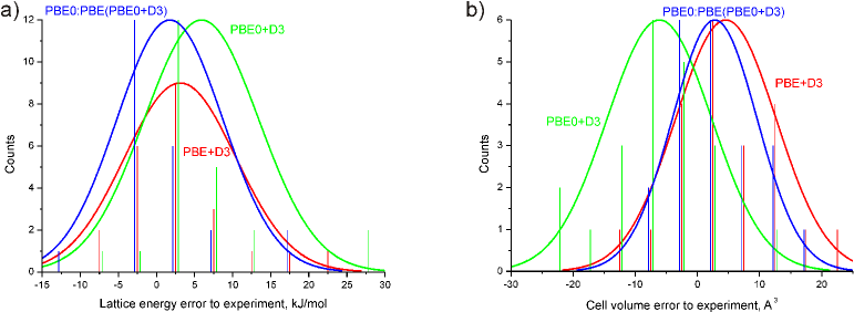
Figure 1: Histograms showing an error distribution of (a) X23 lattice energies and (b) X23-2 cell volumes (see text) with respect to experiment using DFT+D3 and PBE0:PBE(PBE0+D3)

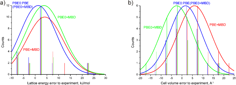
Figure 2: Histograms showing an error distribution of (a) X23 lattice energies and (b) X23-2 cell volumes with respect to experiment using DFT+MBD and PBE0:PBE(PBE0+MBD)

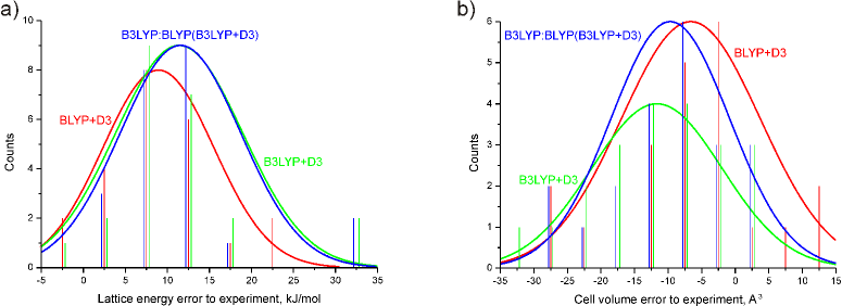
Figure 3: Histograms showing an error distribution of (a) X23 lattice energies and (b) X23-2 cell volumes with respect to experiment using DFT+D3 and B3LYP:BLYP(B3LYP+D3)

This can be seen by the values of Table 5, where the % RMS deviations between PBE0+D3 and PBE+D3 to our PBE0:PBE+D3 method are shown. Here, the PBE0:PBE+D3 values are close to PBE+D3, as indicated by the results displayed. In contrast, the PBE0:PBE+MBD values are much closer to PBE0+MBD. For B3LYP:BLYP+D3, a similar picture emerges, as the RMS errors to BLYP+D3 and B3LYP+D3 are 3.8 and 1.7 kJ/mol, respectively. One reason for this obvious difference is the flat potential energy surface of the PBE+D3 and PBE+MBD methods as well as their hybrid counterparts. As can be seen from Table S10 in the supplementary material, where we performed single-point calculations of our PBE0:PBE+D3 method on both the PBE0+D3 and PBE+D3 structures, the energy differences for these, similar geometries are very small. Thus, the total sum of RMSD between QM:QM and PBE0+D3, PBE+D3 geometries obtained from Kabsch algorithmKabsch (1976, 1978) within ArbAlign codeTemelso et al. (2017) are 0.85 and 0.54$\AA$ correspondingly. The slightly higher lattice energy especially for the PBE0:PBE+MBD values compared to that of the PBE0+MBD structures are due to the k-point grid used for the embedded calculations. Especially the single-point values at the PBE0 and B3LYP structures are extremely close to the optimized ones (0.2 kJ/mol on average), indicating that the potential energy surface of PBE0:PBE is basically flat in that region. It explains the difficulty of PBE0:PBE+D3 to capture the cell volume of the hybrid methods (here, the deviation is much larger than for lattice energies). This implies that for B3LYP+D3, where the dispersion part is much larger, the energy differences are less determined by the functional part and the potential energy surface is steeper. For PBE0+D3 or PBE+D3, the short-range dispersion of the functional appears to play a larger role and thus, the embedded value is closer to PBE+D3. The MBD dispersion in PBE is slightly larger than D3, therefore the PBE0:PBE+MBD values are closer to PBE0+MBD, in contrast to D3.

Thus, B3LYP:BLYP+D3 is very close to B3LYP+D3, whereas PBE0:PBE+MBD are in between PBE and PBE0. As before, PBE0:PBE appears somewhat closer to PBE+D3 and PBE0:PBE+MBD to PBE0+MBD.
Although we are able to reproduce B3LYP+D3 rather well with B3LYP:BLYP+D3, the PBE0:PBE+D3 and PBE0:PBE+MBD methods may need some reparametrization of the dispersion coefficients, as it was done for the HSE+D3 method. Nevertheless, for the monomers and dimers, we automatically achieve the accuracy of hybrid functionals for the introduced method, which may be an important step when comparing different polymorphs.

Table 3: PBE0+MBD: X23 lattice energies calculated with higher and lower k-point grids and respective errors to experiment.

X23 phase	Small	Large	Exp	Small-Exp	Large-Exp
Acetic acid	75.64	74.20	72.8	2.84	1.40
Adamantane	75.49	73.90	69.4	6.09	4.50
Anthracene	106.65	105.13*	112.7	-6.05	-7.57
Benzene	54.52	52.82	55.3	-0.78	-2.48
Carbon dioxide	23.02	22.80	28.4	-5.38	-5.6
Cyanamide	88.90	88.08	79.7	9.2	8.38
Cyclohexane-1,4-dione	93.42	90.29*	88.6	4.82	1.69
Cytosine	159.42	157.80*	162.8	-3.38	-5.00
Ethyl carbamate	90.09	87.30	86.3	3.79	1.00
Formamide	81.21	80.17	79.2	2.01	0.97
Hexamethylenetetramine	86.49	85.34	86.2	0.29	-0.86
Imidazole	90.50	89.10	86.8	3.7	2.30
Naphthalene	79.56	76.82	83.1	-3.54	-6.28
Ammonia	40.45	40.27	37.2	3.25	3.07
Oxalic acid ($\alpha$)	120.25	118.04	96.3	23.95	21.74
Oxalic acid ($\beta$)	120.49	118.58	96.1	24.39	22.48
Pyrazine	60.13	58.77	61.3	-1.17	-2.53
Pyrazole	80.24	78.20*	77.7	2.54	0.50
Succinic acid	135.05	133.16	130.3	4.75	2.86
s-Triazine	55.78	54.02*	61.7	-5.92	-7.68
s-Trioxane	60.93	59.30*	66.4	-5.47	-1.63
Uracil	139.54	135.00*	135.7	3.84	-0.70
Urea	111.84	111.55	102.5	9.34	9.05

* Calculated with a standard (GGA) set of k-points (for its definition - see Table S1). MAE(Small) = 5.93 kJ/mol

MAE(Large) = 5.29 kJ/mol

Table 4: Lattice energy (kJ/mol) and cell volume ($\AA^{3}$) errors of complete X23 and truncated (X23-2)^∗ crystal sets computed by embedded QM:QM and pure QM methods with respect to experimental reference values with Ref_th and without (Ref.) thermal expansion correction^∗∗ applied.

method	lattice energy error	lattice energy % error	cell volume error	cell volume % error	cell volume error	cell volume % error
(dispersion)	RMS / MAE / mean	RMS / mean	RMS /  MAE / mean	RMS / mean	RMS /  MAE / mean	RMS / mean
	Ref. X23		Ref. X23-2		Refth X23-2
PBE+D3	7.8 / 5.3 /  3.1	9.6 / 3.4	7.0 /  5.2 / -3.6	2.8 / -1.1	9.3 /  7.0 / 4.7	4.1 /  1.9
PBE0:PBE(PBE0+D3)	7.0 / 4.1 /  1.8	8.3 / 1.3	8.1 /  6.4 / -5.3	3.0 / -1.7	7.5 / 5.6 / 2.9	3.7 /  1.3
PBE0+D3∗∗∗	9.4 / 6.8 /  5.9	10.7 / 6.4	16.2 /  14.3 / -14.3	4.9 / -4.4	10.4 /  8.4 / -6.0	3.4 / -1.5
PBE+MBDDolgonos et al. (2018)	8.5 / 6.3 /  3.5	10.5 / 3.6	7.1 /  4.6 /  -2.2	2.9 / -0.7	10.0 /  7.7 /  6.1	4.5 / 2.4
PBE0:PBE(PBE0+MBD)	7.6 / 5.1 /  0.6	9.5 /0.3	9.8 /  7.3 /  -6.4	3.3 / -2.0	7.9 /  6.3 /  1.8	3.5 / 1.0
PBE0+MBD∗∗∗	8.8 / 5.9 /  3.2	10.1 / 2.9	13.1 /  11.1 / -10.6	4.1 / -3.3	8.1 /  6.5 / -2.4	3.4/ -0.4
BLYP+D3	11.0 /  9.3/  8.9	13.0 / 10.3	17.6 /  14.8 / -14.8	5.0 / -4.5	12.2 /  9.7 /  -6.5	3.6 / -1.5
B3LYP:BLYP(B3LYP+D3)	13.6 / 11.6 / 11.6	15.6 / 13.7	19.9 /  17.8 /  -17.8	5.8 / -5.6	13.0 /  10.8 / -9.6	3.6 / -2.7
B3LYP+D3∗∗∗	13.6 / 11.4 / 11.4	15.3 / 13.2	22.2 /  19.8 /  -19.8	6.4 / -6.1	15.1 /  12.5 / -11.6	4.1 / -3.2

^∗Pyrazole and s-Triazine are excluded

^∗∗Computed from the explicitly thermally expanded structures obtained with the FIT force fieldNyman et al. (2016)

^∗∗∗ Based on a small set of k-points (see Table S1)

Table 5: Lattice energy (kJ/mol) and cell volume ($\AA^{3}$) errors of X23 crystal set computed by pure QM methods with respect to embedded QM:QM.

method	lattice energy error	lattice energy % error	cell volume error	cell volume % error
(dispersion)	(RMS / mean)	(RMS / mean)	(RMS /  mean)	(RMS /  mean)
PBE+D3	2.4/ 1.4	3.8/ 2.1	3.5/ 2.1	0.9 / 0.6
PBE0+D3∗	4.7 / 4.1	5.5 / 5.0	10.4 / -9.5	2.8 / -2.8
PBE+MBDDolgonos et al. (2018)	3.3/ 2.8	5.0 / 4.0	6.0 / 4.8	1.7 / 1.4
PBE0+MBD∗	2.8 / 2.5	3.8 / 3.3	5.6/ -4.6	1.5/ -1.3
BLYP+D3	3.8 / -2.7	4.1 / -3.0	4.2 / 3.2	1.5 / 1.1
B3LYP+D3∗	1.7 / -0.2	1.6 / -0.4	2.7 / -2.0	0.7 / -0.6

^∗Based on reduced set of k-points (see Table S1)

IV Conclusions

We propose a method for optimization of weakly bound periodic systems based on an embedding QM:QM scheme. In this approach, we combine the energies and gradients from high-level QM fragment calculations with those coming from fast, low-level periodic DFT. Here, we introduce PBE0 embedded into PBE and B3LYP embedded into BLYP as alternative method for hybrid functionals for molecular crystals. The robust calculation of crystal lattice energies and cell volumes makes it the promising tool for further applications, especially when accurate structures and energetics from hybrid functionals are needed.

SUPPLEMENTARY MATERIAL

See supplementary material for detailed lattice energies, cell volumes, reference cell volumes, and k-points.