Non-integrable fermionic chains near criticality.

Abstract

We compute the Drude weight and the critical exponents as functions of the density in non-integrable generalizations of XXZ or Hubbard chains, in the critical zero temperature regime where Luttinger liquid description breaks down and Bethe ansatz cannot be used. Even in the regions where irrelevant terms dominate, no difference between integrable and non integrable models appear in exponents and conductivity. Our results are based on a fully rigorous two-regime multiscale analysis and a recently introduced partially solvable model.

Lattice fermion models Quantum Transport Renormalization group methods

1 Introduction

Understanding whether the behavior of exactly solvable models is generic and persists in presence of integrability-breaking terms is a central issue in physics. Interacting fermionic chains provide an ideal arena, thanks to the presence of Bethe ansatz solvable models, like the XXZ or the Hubbard model, and the fact that cold atoms allow, at least in principle, an experimental verification [1, 2, 3]. Exact solutions provide a rather complete picture, including critical exponents at zero temperature for all densities [4], Mazur bounds for Drude weights (whose finiteness signals an infinite conductivity) at finite temperature [5, 6] and dynamical correlations [7, 8, 9]. In addition, Drude weights can be obtained via dynamical evolution of partitioned systems [10, 11, 12, 13, 14, 15, 16, 17, 18].

Luttinger liquid theory [19] predicts the behavior of the Luttinger model to be generic for non-integrable systems [20]. This was rigorously proved [21] for static zero temperature properties around the half filled band case, where the dispersion relation is essentially linear. These limitations are necessary; solvable models show that non linear dispersion relations produce behaviors different from that of the Luttinger model in the dynamical correlations or at finite temperature; the same is true for static zero temperature properties at low or high densities.

For the same non linear lattice dispersion relation, integrable or non integrable interactions differ by irrelevant terms, usually neglected in field theoretic Renormalization Group (RG) analysis; for instance, the addition of a next to nearest neighbor interaction makes the XXZ model not solvable. The RG irrelevance of these terms does not make them unimportant. On the contrary, it has been proposed that at positive temperature the Drude weight can depend dramatically on the integrability of the interaction [5, 6], in analogy with the classical case [22]. This scenario still lacks confirmation [23, 24, 25, 26, 27, 28]. More generally, irrelevant terms are known to play a crucial role for transport properties. For instance, they ensure the cancellation of all the interaction corrections of the optical conductivity of graphene[29, 30].

The natural question we address here is the following: for which properties is the behavior found in Bethe ansatz solvable models generic even when the Luttinger description breaks down and physics is dominated by irrelevant terms? We answer this question in the case of static zero temperature properties in the low or high density regions, away from Luttinger linear behavior. This is achieved via a two-regime non-perturbative RG scheme that keeps fully into account irrelevant terms. In the second regime, in the spinful case we exploit emerging symmetries by using a recently introduced QFT model [31] with a RG flow exponentially close to the flow of the non integrable chains. This QFT model is partially solvable in the sense that only the density correlations can be obtained in closed form.

We find that the critical exponents, in the low or high density limit, tend to their non interacting value in the spinless case, while in the spinful case their limiting value depends strongly on the interaction. In both cases the Drude weight behave essentially as in the non interacting case. In the special case of solvable interactions, Bethe ansatz results are recovered.

Our analysis shows that there is no qualitative difference between integrable and non integrable models at zero temperature; the exponents have a similar behavior and the conductivity is infinite, and the limiting value of the Drude weight is the same. This is true notwithstanding the fact that near criticality the physics is completely dominated by the irrelevant terms. As soon as $T\not=0$, it is common belief that a completely different behavior of the Drude weight occurs, being it vanishing or not depending on integrability. The fact that integrability breaking perturbations are unable to produce any difference at $T=0$, even in regions where irrelevant terms dominate, makes it also possible a scenario in which a difference is visible only at not too small temperatures.

2 Main results

We consider a model of interacting fermions with Hamiltonian

$$H= -\frac{1}{2}\sum_{x,\sigma}(a^{+}_{x,\sigma}a^{-}_{x+1,\sigma}+c.c.)-\mu\sum_{x,\sigma}a^{+}_{x,\sigma}a^{-}_{x,\sigma}$$

$$+\lambda\sum_{\begin{subarray}{c}x,y\\ \sigma,\sigma^{\prime}\end{subarray}}w(x-y)a^{+}_{x,\sigma}a^{-}_{x,\sigma}a^{+}_{y,\sigma^{\prime}}a^{-}_{y,\sigma^{\prime}}$$ (1)

where $a^{\pm}_{x,\sigma}$ are fermionic creation or annihilation operators, $\sigma$ is the spin ($\sigma=0$ in the spinless case and $\sigma=\uparrow,\downarrow$ in the spinning case), $x$ are points on a one dimensional lattice and $w(x)$ is a short range potential such that $\sum_{x}|x|^{\alpha}|w(x)|<\infty$ for some $\alpha>0$. In the spinless case with $w(x-y)=\delta_{x,y+1}$ the system reduces to the $XXZ$ model and in the spinning case with $\lambda w(x-y)=U\delta_{x,y}$ it reduces to the Hubbard model. For other choices of the interaction no solution is known.

The truncated Euclidean correlations are

$$\langle O_{{\bf x}_{1}}...O_{{\bf x}_{n}}\rangle=\langle\mathbf{T}(O_{{\bf x}_{1}}...O_{{\bf x}_{n}})\rangle_{T}\,,$$

where $\mathbf{T}$ is the time ordering operator, ${\bf x}=(x_{0},x)$, $O_{\bf x}=e^{Hx_{0}}O_{x}e^{-Hx_{0}}$ and $\langle\cdot\rangle_{T}$ are the thermodynamic truncated averages. Finally $S({\bf x}-{\bf y})=\langle a^{-}_{\bf x}a^{+}_{\bf y}\rangle$ denotes the 2-point correlation function.

The density is $\rho_{x}=\sum_{\sigma}a^{+}_{x,\sigma}a^{-}_{x,\sigma}$ and the current is defined via the continuity equation that gives

$$j_{x}=\frac{1}{2i}\sum_{\sigma}(a^{+}_{x+1,\sigma}a^{-}_{x,\sigma}+a^{+}_{x,\sigma}a^{-}_{x+1,\sigma})\,.$$

Writing ${\bf p}=(p_{0},p)$, the (Euclidean) zero temperature Drude weight $D$ and the susceptibility $\kappa$ are given by

$$\kappa=\lim_{p\to 0}\lim_{p_{0}\to 0}\langle\hat{\rho}_{\bf p}\hat{\rho}_{-{\bf p}}\rangle_{T}\quad\mathrm{and}\quad D=\lim_{p_{0}\to 0}\lim_{p\to 0}D({\bf p})$$

with $D({\bf p})=\langle\hat{j}_{\bf p}\hat{j}_{-{\bf p}}\rangle_{T}+\Delta$ and

$$\Delta=-\frac{1}{2}\sum_{\sigma}\langle a^{+}_{x,\sigma}a^{-}_{x+1,\sigma}+a^{+}_{x+1,\sigma}a^{-}_{x,\sigma}\rangle\,.$$

Here $\hat{f}({\bf p})$ represents the Fourier transform of $f({\bf x})$. A Ward Identity (WI) gives $p_{0}^{2}\langle\hat{\rho}_{\bf p}\hat{\rho}_{-{\bf p}}\rangle=4\sin^{2}p/2D({\bf p})$ which implies that

$$\lim_{p\to 0}\lim_{p_{0}\to 0}D({\bf p})=\lim_{p_{0}\to 0}\lim_{p\to 0}\langle\hat{\rho}_{\bf p}\hat{\rho}_{-{\bf p}}\rangle=0\,.$$

Note that $D({\bf p})$ is not continuous at ${\bf p}=0$ and it is essential to take the limits in the correct order. Moreover the limit $p_{0}\to 0$ should be taken along the imaginary axis, but Wick rotation holds for this model [32].

Theorem Consider the Hamiltonian (1) with $\mu=\mu_{R}+\nu(\lambda,r)$ and $\mu_{R}=-\cos p_{F}=\pm 1\mp r$. Then we have

$$D=\frac{Kv}{\pi}\quad\mathrm{and}\quad\kappa=\frac{K}{\pi v}$$

where:

$\bullet$ In the spinless case for $|\lambda|$ small we have

$$\nu(\lambda,r)=2\lambda\hat{w}(0)\frac{p_{F}}{\pi}+O(\lambda r)$$

while

$$K= \frac{1-\tau}{1+\tau}\,,$$

$$v= \sin p_{F}(1+O(\lambda r^{\vartheta}))\,,$$

$$\tau= \lambda\frac{\hat{w}(0)-\hat{w}(2p_{F})}{2\pi v}+O(\lambda^{2}r^{\vartheta})\,,$$

with $\vartheta\in(1/3,1/2)$;

$\bullet$ In the spinful case for $\tilde{\lambda}=\frac{\lambda}{\sin p_{F}}\geq 0$ small we have $\nu(\lambda,r)=O(\tilde{\lambda}\sqrt{r})$ while

$$K=\sqrt{\frac{(1-2\nu_{\rho})^{2}-\nu_{4}^{2}}{(1+2\nu_{\rho})^{2}-\nu_{4}^{2}}}\quad v^{2}=\bar{v}^{2}\frac{(1+\nu_{4})^{2}-4\nu_{\rho}^{2}}{(1-\nu_{4})^{2}-4\nu_{\rho}^{2}}$$

where

$$\bar{v}= \sin p_{F}(1+O(\tilde{\lambda}r^{\vartheta})+O(\tilde{\lambda}^{2}))\,,$$

$$\nu_{4}= \tilde{\lambda}\frac{\hat{w}(0)}{2\pi}+O(\tilde{\lambda}^{2})\,,$$

$$\nu_{\rho}= \frac{\tilde{\lambda}}{2\pi}(\hat{w}(0)-\frac{\hat{w}(2p_{F})}{2})+O(\tilde{\lambda}^{2})\,.$$

In both cases, $S({\bf x}-{\bf y})$ decays for large distance as $|{\bf x}|^{1+\eta}$ with $2\eta=K+K^{-1}-2$.

In the Theorem $r$ is a parameter that measures the distance of $\mu$ from the critical chemical potential $\mu_{c}$. In the spinless case $\mu_{c}$ is shifted by the interaction and we get $\mu_{c}=1+2\lambda\hat{w}(0)$ for $\mu_{R}=1$ and $\mu_{c}=-1$ for $\mu_{R}=-1$. In the $XXZ$ chain $h_{c}+\lambda=\mu_{c}$. When $r\to 0$ we get $K\to 1$ and $D/\sin p_{F}\to\frac{1}{\pi}$, that is the critical exponent and the Drude weight tend to their non-interacting values. Fig. 1 shows the behavior of $D$ and $K$ as function of the density close to the critical point; in the XXZ case it closely reproduces the features found by the exact solution, see e.g. Fig. 1 in [33] or Fig. 1 in [34].

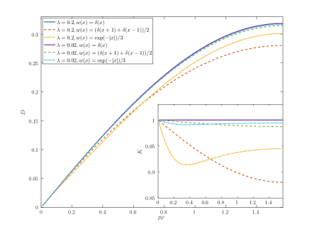
Figure 1: The main graph is the Drude weight $D$ at fixed $\lambda$ in the spinless case. The inset shows $K$.

In the spinful case we rescale the interaction as $\lambda=\tilde{\lambda}\sin p_{F}$. In term of $\tilde{\lambda}$ our results hold uniformly in $r$. In contrast with the spinless case, the theory is strongly interacting since at criticality we have $K\to 1-\tilde{\lambda}\hat{w}(0)/\pi+O(\tilde{\lambda}^{2})$. A remarkable cancellation takes place in the Drude weight and $D$ behaves as in the non interacting case when $r\to 0$ (at least up to $O(\tilde{\lambda}^{2})$ terms), that is

$$\frac{D\pi}{\bar{v}}=\frac{1+\nu_{4}-2\nu_{\rho}}{1-\nu_{4}+2\nu_{\rho}}\sim 1$$

for $r\sim 0$. Such a behavior is present in the Hubbard model, but it is proven here to be a generic feature. It was missed in previous attempts based of field theoretic RG methods. Fig. 2 shows the behavior of $D$ and $K$ for integrable and non integrable interactions, as function of $\lambda$ and $\tilde{\lambda}$. In the Hubbard case Fig. 2 reproduces Bethe ansatz result (e.g. Fig. 9.2, 9.3 of [4] or Fig. 13, 14 of [35]).

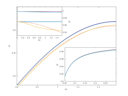
Figure 2: The main graph is the Drude peak $D$ at fixed $\lambda$ for the spinful case. The upper insets shows $K$ at fixed $\tilde{\lambda}$ while the lower inset shows $K$ as a function of $\lambda$. Colors and dashes are as in Fig. 1

3 RG analysis: the quadratic regime

We write the Euclidean correlations in terms of a Grassmann integral

$$e^{W(A,\phi)}=\int P(da)e^{-{\cal V}-\nu N+B(A,\phi)}$$

where $P(da)$ is a Grassmann integration on the Grassmann algebra generated by the variables $a^{\pm}_{{\bf x},\sigma}$ with propagator

$$g({\bf x}-{\bf y})=\frac{1}{4\pi^{2}}\int e^{-i{\bf k}({\bf x}-{\bf y})}\hat{g}({\bf k})\,d{\bf k}$$

where

$$\hat{g}({\bf k})=\frac{1}{-ik_{0}-\cos k+\cos p_{F}}\,.$$

Moreover ${\cal V}$ is the interaction and $\nu N=\nu\int d{\bf x}\,a^{+}_{{\bf x},\sigma}a^{-}_{{\bf x},\sigma}$ is a counterterm introduced to take into account the renormalization of the chemical potential, that is we write $\mu=\mu_{R}+\nu$ with $\mu_{R}\equiv\cos p_{F}$. Finally $B(A,\phi)$ is a source term. Differentiating $W(A,\phi)$ with respect to $\phi$ produces correlations of fermionic fields, while differentiating with respect to $A$ produces correlations of currents or densities.

The starting point of the RG analysis is the decomposition

$$\hat{g}({\bf k})=\sum_{h=-\infty}^{1}\hat{f}_{h}({\bf k})\hat{g}({\bf k})=\sum_{h=-\infty}^{1}\hat{g}^{(h)}({\bf k})$$ (2)

where $\hat{f}_{h}({\bf k})$ is a compact support function non vanishing only for $\sqrt{k_{0}^{2}+(\cos k-\cos p_{F})^{2}}\sim 2^{h}$, see Fig. 3. From eq.(2) and the prperties of Grassmanian integrations we have that we can write $a^{\pm}_{{\bf x},\sigma}=\sum_{h=-\infty}^{1}a^{h,\pm}_{{\bf x},\sigma}$ with $P(da)=\prod_{h=-\infty}^{1}P(da^{h})$. This decomposition naturally leads to identify two regions, separated by the energy scale $2^{h^{*}}\sim r$; in the region where the energy is greater $r$ the dispersion relation is essentially quadratic, while for smaller energies it is essentially linear with a slope of $\sin p_{F}\sim\sqrt{r}$.

In the high energy region where $h\geq h^{*}$ the single scale propagator satisfies the scaling relations $g^{(h)}({\bf x})\sim 2^{h/2}g^{(0)}(2^{h}x_{0},2^{h/2}x)$ and the scaling dimension is $D^{1}=3/2-l/4-m/2$ where $l$ is the number of $a$ fields and $m$ the number of $A$ fields.

We focus on the $A=\phi=0$ case. We define the effective potential on scale $h$ recursively as

$$V^{h}(a^{\leq h})=\log\int P(da^{h})e^{V^{h+1}(a^{\leq h+1})}$$

where $a^{\leq h}=\sum_{k=-\infty}^{h}a^{k}$. It can be written as

$$V^{h}={\cal L}V^{h}+{\cal R}V^{h}\,,$$

where ${\cal R}V^{h}$ is sum of all irrelevant terms, that is monomials in the fields with $D^{1}<0$ while

$${\cal L} V^{h}=2^{\frac{h}{2}}\lambda_{h}F_{\lambda}+2^{h}\nu_{h}\sum_{\sigma}\int d{\bf x}\,a^{+,\leq h}_{{\bf x},\sigma}a^{-,\leq h}_{{\bf x},\sigma}+$$ (3)

$$i_{h}\sum_{\sigma}\int d{\bf x}\,a^{+,\leq h}_{{\bf x},\sigma}\partial_{0}a^{-,\leq h}_{{\bf x},\sigma}+\delta_{h}\sum_{\sigma}\int d{\bf x}\,a^{+,\leq h}_{{\bf x},\sigma}\partial^{2}a^{-,\leq h}_{{\bf x},\sigma}$$

where

$$F_{\lambda}=\int d{\bf x}\,a^{+,\leq h}_{{\bf x},\uparrow}a^{-,\leq h}_{{\bf x},\uparrow}a^{+,\leq h}_{{\bf x},\downarrow}a^{-,\leq h}_{{\bf x},\downarrow}$$

in the spinful case and $F_{\lambda}=0$ if the fermions are spinless. Notice the absence of the term $\int a^{+}_{{\bf x},\sigma}\partial a^{-}_{{\bf x},\sigma}d{\bf x}$ and of local terms with six fields due to parity and the Pauli principle, respectively.

After integrating the field $a^{h}$ we obtain $V^{h-1}$ as a sum of monomials in the fields, that is

$$V^{h-1}(a^{\leq h-1})=\int W_{l}^{h-1}({\bf x}_{1},\ldots,{\bf x}_{l})\prod_{i=1}^{l}a^{\leq h-1}_{{\bf x}_{i}}$$

where $W^{h-1}_{l}$ is expressed as a series in the running coupling constant (r.c.c.) $\bm{\eta}_{h}=(\nu_{k},i_{k},\delta_{k},\lambda_{k})$ (with $\lambda_{k}\equiv 0$ in the spinless case), $k\geq h$. We can now write $V^{h-1}={\cal L}V^{h-1}+{\cal R}V^{h-1}$ as in (3) with $h-1$ replacing $h$ and use the local terms to compute the r.c.c. on scale $h-1$. This produces an expansion of the kernels $W_{l}^{h}$ in in terms of the r.c.c.. Calling $\epsilon_{h}=\max_{k>h}|\bm{\eta}_{k}|$, we get

$$||W_{l}^{h-1}||\leq 2^{h(3/2-l/4)}\sum_{n}C^{n}\epsilon_{h}^{n}$$

Convergence in the r.c.c. follows from determinant bounds [36], which imply convergence in $\lambda$ if the r.c.c. remain close to their initial value during RG iteration.

The above construction gives the recursive relation

$$\bm{\eta}_{h-1}=\bm{\eta}_{h}+\beta^{h}(\bm{\eta}_{h},\ldots,\bm{\eta}_{0})\,.$$

The flow generated by $\beta^{h}$ can be analyzed rigorously as in [36]. The main observation is that at $r=0$ all graphs with a closed fermionic loop vanish while the tadpole graph gives the shift of the chemical potential. Therefore in the spinless case we get $|i_{h}|,|\delta_{h}|\leq Cr^{\vartheta}|\lambda|$ where the factor $r^{\vartheta}$ due to the irrelevance of the quartic terms. Similarly the contribution to $\nu$ are the tadpole graph plus $O(\lambda r)$.

In the spinful case we must also consider $\lambda_{h}$ which obeys the recursive relation $\lambda_{h-1}=2^{\frac{1}{2}}\lambda_{h}-a\lambda_{h}^{2}+O(\lambda_{h}^{3})$ with $a>0$, from which $|\lambda_{h^{*}}|\leq C|\tilde{\lambda}|$. We thus see a non trivial fixed point that lie outside our convergence radius. For the other r.c.c. we get $|i_{h^{*}}|,|\delta_{h^{*}}|\leq Cr^{\vartheta}|\lambda|+O(\tilde{\lambda}^{2})$ while the contribution to $\nu$ are the tadpole graph plus $O(\lambda r)+O(\tilde{\lambda}^{2})$, see also Appendix A. This is due to the lack of the dimensional gains of the spinless case for graphs of higher order.

Figure 3: Schematic representation of the support $A_{h}$ of the propagator $g^{(h)}({\bf k})$ as a function of $h$.

4 RG analysis: the linear regime

After the integration of the fields $a^{1},a^{0},\ldots,a^{h^{*}}$ we arrive to a functional integral of the form $\int P(da^{\leq h^{*}})e^{-{\cal V}^{h^{*}}(a)}$, where $P(da^{\leq h^{*}})$ has a propagator that depends only on the momenta in two disconnected regions around the 2 Fermi points $(0,\pm p_{F})$, see Fig. 3. Therefore we write $a^{\leq h^{*}}$ as sum of 2 independent fields

$$a^{\leq h^{*}}=\sum_{\omega=\pm}e^{i\omega p_{F}x}a^{\leq h^{*}}_{\omega,{\bf x}}$$

with propagator

$$\hat{g}^{(\leq h^{*})}_{\omega}({\bf k})=\frac{\tilde{f}_{\leq h^{*}}({\bf k})}{-ik_{0}+\omega v_{h^{*}}k}+\hat{r}^{h^{*}}({\bf k})\,,$$

where $v_{h^{*}}=O(\sqrt{r})$, and $\tilde{f}_{\leq h^{*}}({\bf k})$ is different from 0 only if $k_{0}^{2}+v_{h^{*}}^{2}k^{2}\leq 2^{h^{*}}$. Finally $\hat{r}({\bf k})$ is a bounded correction. In this case the scaling dimension is $D^{2}=2-l/2$; we write again $V^{h}={\cal L}V^{h}+{\cal R}V^{h}$, where ${\cal R}V^{h}$ contains all terms with negative scaling dimension while ${\cal L}V^{h}$ contains $\nu_{h}$, the renormalization of the chemical potential, and the quartic terms (quadratic marginal terms produce the wave function renormalization $Z_{h}$ and the renormalized Fermi velocity $v_{h}$). In the spinless case the quartic local terms have the form $\lambda_{h}\int d{\bf x}a^{+,\leq h}_{{\bf x},+}a^{-,\leq h}_{{\bf x},+}a^{+,\leq h}_{{\bf x},-}a^{-,\leq h}_{{\bf x},-}$ with

$$\lambda_{h^{*}}=\lambda(\hat{w}(0)-\hat{w}(2p_{F}))+$$

$$\ \ \sum_{k=h^{*}}^{0}(W_{4}^{k}(p_{F},p_{F},-p_{F},-p_{F})-W_{4}^{k}(p_{F},-p_{F},-p_{F},p_{F}))$$

Due to the parity of the interaction, the first term is $O(\lambda r)$ while the second is close to $p_{F}^{2}\partial^{2}W_{4}^{k}$. Since

$$\sum_{k=h^{*}}^{0}|\partial^{2}W_{4}^{k}|\leq\sum_{k=h^{*}}^{0}\lambda^{2}2^{h(-1/2+\vartheta)}\leq C\lambda^{2}r^{-1/2+\vartheta}$$

we get $\lambda_{h^{*}}\sim O(\lambda r^{\frac{1}{2}+\vartheta})$, so that it vanishes as $r\to 0$. In the spinful case there are three local quartic terms (if $p_{F}\not=\pi/2$):

• $g_{1,h}\int a^{+}_{{\bf x},\omega,\sigma}a^{-}_{{\bf x},-\omega,\sigma}a^{+}_{{\bf x},-\omega,\sigma^{\prime}}a^{-}_{{\bf x},\omega,\sigma^{\prime}}$ with $g_{1,h^{*}}=2^{h^{*}/2}(2\tilde{\lambda}\hat{w}(2p_{F})+O(\tilde{\lambda}^{2}))$ where the $2^{h^{*}/2}$ comes from the scaling dimension;

• $g_{2,h}\int a^{+}_{{\bf x},\omega,\sigma}a^{-}_{{\bf x},\omega,\sigma}a^{+}_{{\bf x},-\omega,\sigma^{\prime}}a^{-}_{{\bf x},-\omega,\sigma^{\prime}}$ with $g_{2,h^{*}}=2^{h^{*}/2}(2\tilde{\lambda}w(0)+O(\tilde{\lambda}^{2}))$;

• $g_{4,h}\int a^{+}_{{\bf x},\omega,\sigma}a^{-}_{{\bf x},\omega,\sigma}a^{+}_{{\bf x},\omega,\sigma^{\prime}}a^{-}_{{\bf x},\omega,\sigma^{\prime}}$ with $g_{4,h^{*}}=2^{h^{*}/2}(2\tilde{\lambda}w(0)+O(\tilde{\lambda}^{2}))$.

The integration over the time variables produces a factor $v^{-n+1}$ which is compensated by the $v^{n}$ of the coupling, so that the convergence radius (in $\lambda$ for the spinless case or $\tilde{\lambda}$ for the spinful case) is $r$ independent. Observe that the small factor in the effective coupling is produced essentially by Pauli principle in the spinless case, while it follows from our choice $\lambda=\tilde{\lambda}\sin p_{F}$ in the spinful case.

Finally we have to discuss the flow of the running coupling constants. The single scale propagator $\hat{g}^{h}({\bf k})$ is sum of of a ”relativistic” part

$$\hat{g}^{h}_{\omega,rel}({\bf k})=\frac{1}{Z_{h}}\frac{\tilde{f}_{h}({\bf k})}{-ik_{0}+\omega v_{h}k}$$

and a correction $\hat{r}^{h}({\bf k})$, smaller by a factor $\frac{2^{h}}{v^{2}_{h^{*}}}$, that takes into account the non linear corrections to the dispersion relation. In the spinless case the beta functions for $\lambda_{h}$ and $v_{h}$ are asymptotically vanishing (i.e. the only contributions come from the corrections $\hat{r}^{h}$) while

$$|\beta_{\lambda}^{h}|\leq C\frac{\lambda^{2}_{h}}{v_{h^{*}}}\frac{2^{h}}{v^{2}_{h^{*}}}\quad\mathrm{and}\quad|\beta_{\delta}^{h}|\leq C\lambda_{h}\frac{2^{h}}{v^{2}_{h^{*}}}\,.$$

Thus we get $|\lambda_{h}|\leq C\lambda r^{1/2+\vartheta}$ while $v_{-\infty}=\sin p_{F}(1+O(\lambda r^{\vartheta}))$. Finally we have $Z_{h}\sim Z_{h^{*}}2^{-\eta h}$ with $\eta=\eta_{i}(\frac{\lambda_{-\infty}}{v_{-\infty}})$, see also Appendix B.

In the spinful case if $\lambda>0$, we get $g_{2,h}\to g_{2,-\infty}$ and $g_{4,h}\to g_{4,-\infty}$ with $g_{2,-\infty}=g_{2,h^{*}}-g_{1,h^{*}}/2+O(\tilde{\lambda}^{2}r^{1/2})$ and $g_{4,-\infty}=g_{4,h^{*}}+O(\tilde{\lambda}^{2}r^{1/2})$. Finally we have $g_{1,h}\sim\frac{g_{1,h^{*}}}{1-ag_{1,h^{*}}(h-h^{*})}\to 0$ as $h\to-\infty$. Similarly we get $\bar{v}=\sin p_{F}(1+O(\tilde{\lambda}r^{\vartheta})+O(\tilde{\lambda}^{2}))$.

5 Emerging Chiral model

Here we focus on the spinful case, since the spinless one is a special case of the following discussion. In the second regime a description of relativistic chiral fermions emerges, up to irrelevant terms, and one needs to exploits its symmetries. A way to do that is to introduce a reference model whose parameters can be fine tuned so that the difference between the running coupling constants of the non integrable chain and those of the reference model is small. The somewhat natural choice of the Luttinger model does not work, as the difference produced by the $g_{1}$ coupling vanishes in a non summable way.

We introduce a model [31] of fermions $\psi^{\pm}_{\omega,\sigma}$ $\omega=\pm$ with propagator

$$\hat{g}^{h}_{\omega,chi}({\bf k})=\frac{1}{Z}\frac{\tilde{f}_{\leq N}({\bf k})}{-ik_{0}+\omega vk}$$

and interaction given by ${\cal V}=\bar{g}_{1}F_{1}+\bar{g}_{2}F_{2}+\bar{g}_{4}F_{4}$ where

$$F_{1} =\frac{1}{2}\sum_{\omega,\sigma,\sigma^{\prime}}\int\tilde{w}({\bf x}-{\bf y})\psi^{+}_{{\bf x},\omega,\sigma}\psi^{-}_{{\bf x},\omega,\sigma^{\prime}}\psi^{-}_{{\bf y},-\omega,\sigma}\psi^{+}_{{\bf y},-\omega,\sigma^{\prime}}$$

$$F_{2} =\frac{1}{2}\sum_{\omega,\sigma,\sigma^{\prime}}\int\tilde{w}({\bf x}-{\bf y})\psi^{+}_{{\bf x},\omega,\sigma}\psi^{-}_{{\bf x},\omega,\sigma}\psi^{-}_{{\bf y},-\omega,\sigma^{\prime}}\psi^{+}_{{\bf y},-\omega,\sigma^{\prime}}$$

$$F_{4} =\frac{1}{2}\sum_{\omega,\sigma,\sigma^{\prime}}\int\tilde{w}({\bf x}-{\bf y})\psi^{+}_{{\bf x},\omega,\sigma}\psi^{-}_{{\bf x},\omega,\sigma}\psi^{-}_{{\bf y},\omega,\sigma^{\prime}}\psi^{+}_{{\bf y},\omega,\sigma^{\prime}}\,.$$

Here $\tilde{w}({\bf x})$ is a short range interaction, with range $r_{0}$ and $\hat{w}(0)=1$. Setting

$$\tilde{\jmath}_{0,{\bf x}}=\sum_{\omega}\tilde{\rho}_{\omega,{\bf x}}\,,\qquad\tilde{\jmath}_{1,{\bf x}}=\sum_{\omega}\omega\tilde{\rho}_{\omega,{\bf x}},$$

with $\tilde{\rho}_{\omega,{\bf x}}=\sum_{\sigma}\psi^{+}_{\omega,\sigma}\psi^{-}_{\omega,\sigma}$, we get the WI for the fermionic correlations

$$-ip_{0}A_{0}\langle\hat{\tilde{\jmath}}_{0,{\bf p}} \hat{\psi}^{-}_{{\bf k}+{\bf p},\sigma}\hat{\psi}^{+}_{{\bf k},\sigma}\rangle_{T}+$$

$$pvA_{1} \langle\hat{\tilde{\jmath}}_{1,{\bf p}}\hat{\psi}^{-}_{{\bf k}+{\bf p},\sigma}\hat{\psi}^{+}_{{\bf k},\sigma}\rangle_{T}=$$ (4)

$$\frac{1}{Z}\left[\langle\hat{\psi}^{-}_{{\bf k}+{\bf p},\sigma}\hat{\psi}^{+}_{{\bf k}+{\bf p},\sigma}\rangle_{T}-\langle\hat{\psi}^{-}_{{\bf k},\sigma}\hat{\psi}^{+}_{{\bf k},\sigma}\rangle_{T}\right]$$

where $A_{0}=(1-\nu_{4}-2\nu_{\rho}),A_{1}(1+\nu_{4}-2\nu_{\rho})$, $\nu_{4}=\bar{g}_{4}/4\pi v$ and $\nu_{\rho}=(\bar{g}_{2}-\bar{g}_{1}/2)/4\pi v$. Similarly, if $\tilde{P}_{\omega}=-ip_{0}+\omega vp$, the density correlations verify

$$\tilde{P}_{\omega}\langle\hat{\tilde{\rho}}_{{\bf p},\omega} \hat{\tilde{\rho}}_{-{\bf p},\omega^{\prime}}\rangle_{T}-\nu_{4}\tilde{P}_{-\omega}\langle\hat{\tilde{\rho}}_{{\bf p},\omega}\hat{\tilde{\rho}}_{-{\bf p},\omega^{\prime}}\rangle_{T}-$$ (5)

$$-2\nu_{\rho}\tilde{P}_{-\omega}\langle\hat{\tilde{\rho}}_{{\bf p},-\omega}\hat{\tilde{\rho}}_{-{\bf p},\omega^{\prime}}\rangle_{T}=-\delta_{\omega,\omega^{\prime}}\frac{\tilde{P}_{-\omega}}{2\pi Z^{2}}$$

Note in the above WI the presence of the anomalies, that is te terms in $\nu_{\rho}$ and $\nu_{4}$, which are linear in the couplings $\bar{g}_{i}$. The model differs from the Luttinger model for the presence of the $\bar{g}_{1}$ term; it is however defined so that it is invariant under the chiral phase transformation

$$\psi^{\pm}_{{\bf x},\omega,\sigma}\to e^{\pm i\alpha_{{\bf x},\omega}}\psi^{\pm}_{{\bf x},\omega,\sigma}$$

which imply, thanks to (5), that the density correlations can be explicitly computed even if the model is not solvable, see [21, 31]. We choose $\tilde{w}$ of the form $\tilde{w}({\bf x})=\bar{w}(x^{2}+x_{0}^{2}/v^{2})$ where $\bar{w}$ has range $r_{0}=2^{-h^{*}}$ and satisfies $\int d{\bf x}|\tilde{w}({\bf x})|=1$. It acts as an ultraviolet cut-off that allow us to integrate safely the scales $h\geq h^{*}$ and arrives to an effective potential $\overline{V}^{h^{*}}$, differing from $V^{h^{*}}$ discussed in the previous section by irrelevant terms. We can choose the bare parameters $\bar{g}_{i},v$ of the reference model so that its running coupling constants differ from those of model (1) by exponentially decaying terms $O(2^{\vartheta h})$ and the ratio of the $Z$ tends to $1$; this is achieved by choosing $\bar{g}_{i}=g_{i,h^{*}}+O(\sqrt{r}\tilde{\lambda}^{2}))$ and $v=\sin p_{F}(1+O(\tilde{\lambda}r^{\vartheta})+O(\tilde{\lambda}^{2}))$. This implies that

$$D({\bf p})=\frac{Z_{1}^{2}}{Z^{2}}\langle\hat{\tilde{\jmath}}_{1,{\bf p}}\hat{\tilde{\jmath}}_{1,-{\bf p}}\rangle_{T}+R_{0}({\bf p})$$ (6)

where $Z_{1}$ is the current wave function normalization and $R_{0}({\bf p})$ is a continuous function in ${\bf p}$ (in contrast with the first addend in the r.h.s.); we use the WI $\lim_{p\to 0}\lim_{p_{0}\to 0}D({\bf p})=0$ to fix $R_{0}(0)$ so that we get

$$D({\bf p})=\frac{Z_{1}^{2}}{\pi Z^{2}vv_{1}}\frac{[(1+\nu_{4}+2\nu_{\rho})+v_{2}^{2}(1-\nu_{4}-2\nu_{\rho})]p_{0}^{2}}{p_{0}^{2}+v_{2}^{2}v^{2}p^{2}}$$

with $v_{2}^{2}=\frac{(1+\nu_{4})^{2}-4\nu_{\rho}^{2}}{(1-\nu_{4})^{2}-4\nu_{\rho}^{2}}$, $v_{1}=(1+\nu_{4})^{2}-4\nu_{\rho}^{2}$. The identity

$$\langle j_{{\bf p}}a^{-}_{{\bf k}+{\bf p}_{F},\sigma}a^{+}_{{\bf k}+{\bf p}+{\bf p}_{F},\sigma}\rangle_{T}=Z_{1}\langle\tilde{j}_{1,{\bf p}}\psi^{-}_{{\bf k}+{\bf p},\sigma}\psi^{+}_{{\bf k},\sigma}\rangle_{T}$$

allows us to fix $Z_{1},Z$; indeed comparing (4) with the WI for the chain

$$-ip_{0}\langle\hat{\rho}_{\bf p}\hat{a}^{-}_{{\bf k},\sigma}a^{+}_{{\bf k}+{\bf p},\sigma}\rangle_{T}+ p\langle\hat{j}_{\bf p}\hat{a}^{-}_{{\bf k},\sigma}a^{+}_{{\bf k}+{\bf p},\sigma}\rangle_{T}$$ (7)

$$= \langle\hat{a}^{-}_{{\bf k},\sigma}a^{+}_{{\bf k},\sigma}\rangle_{T}-\langle\hat{a}^{-}_{{\bf k}+{\bf p},\sigma}a^{+}_{{\bf k}+{\bf p},\sigma}\rangle_{T}$$

we get the consistency relations

$$\frac{Z_{1}}{Z}=v(1+\nu_{4}-2\nu_{\rho})\,.$$

Proceeding in a similar way for the susceptibility we obtain the expressions in the Theorem.

6 Conclusions

We analyze non integrable generalizations of XXZ and the Hubbard chain in the low and high density regimes where the Luttinger description breaks down. Our methods are based on a multiscale decomposition of the propagator of the theory and are able to take into account, in a rigorous and quantitative way, the irrelevant terms normally neglected in RG analysis. Our main conclusion is that no qualitative difference between solvable and non solvable models are seen in exponents and conductivity at zero temperature, even in regions where Luttinger liquid description is not valid and the physics is completely dominated by irrelevant terms. In particular the anomalous critical exponents vanishes or not depending on the spinless or spinful nature of fermions, and the Drude weight tends to the same non interacting values in both cases.

It is common belief that the Drude weight is zero in the presence of non integrable interactions, while still non zero for integrable ones, as soon as $T\not=0$. However, the fact that at $T=0$ integrability breaking terms do not produce any difference in the transport properties, even in regimes where irrelevant terms dominate, makes it also possible a scenario where breaking of integrability effects in transport may matters only at not too low temperature [37].

7 Appendix A: Flow of the running coupling constants in the quadratic regime

We give some extra detail on the flow of the r.c.c. in the quadratic regime. Note that at $r=0$ and $T=0$ we have

• empty band case: $p_{F}=0$, $e(k)=-\cos k+1$, and

  $$g({\bf x})=\chi(x_{0}>0)\int_{-\pi}^{\pi}\frac{dk}{2\pi}e^{-ikx-e(k)x_{0}}$$

• filled band case: $p_{F}=\pi$, $e(k)=-\cos k-1$, and

  $$g({\bf x})=-\chi(x_{0}\leq 0)\int_{-\pi}^{\pi}\frac{dk}{2\pi}e^{-ikx-e(k)x_{0}}$$

Therefore all the graphs with order greater than $1$ with two external lines are vanishing if computed at the Fermi points and $r=0$. Indeed all one particle reducible graphs are vanishing due to the support properties of the propagator. This implies that there is always a closed fermionic loop which vanishes as the propagator is proportional to $\chi(x_{0}>0)$ or $\chi(x_{0}\leq 0)$. At first order there are two contributions: the tadpole graph at $r=0$ contributes only to $\nu$ and gives $2\lambda\hat{w}(0)p_{F}/\pi$ with $p_{F}=0,\pi$; the other graph is vanishing for non local interactions (local potential does not contribute) since $v({\bf x}-{\bf y})g({\bf x}-{\bf y})$ is proportional to $v(x,y)\delta_{x,y}=0$.

The flow equations for $i_{h},\delta_{h}$ have the form $i_{h-1}=i_{h}+\beta_{i}^{h}$, $\delta_{h-1}=\delta_{h}+\beta_{i}^{h}$. In the spinless case the fact that there are no quartic running coupling constants produce an improvement of $O(2^{h\vartheta})$ with respect to the dimensional bound . As we noticed above all the contributions with two external lines computed at the Fermi points are vanishing for $r=0$, except the tadople which contributes only to $\nu_{h}$. There is therefore a gain $r2^{-h}$ in the beta function for $z,\delta$, and a further gain $2^{h\vartheta}$ (due to the irrelevance of the quartic terms if the order is greater then $1$ and to the fact that the derivative can be applied on the interaction at first order), so we get $|i_{h}|,|\delta_{h}|\leq\sum_{k=h}^{1}C|\lambda|r2^{-k}2^{k\vartheta}$ and finally $z_{h^{*}},\delta_{h^{*}}=O(\lambda r^{\vartheta})$. The same argument can be used for the renormalization of the chemical potential $\nu_{h}$ and $\nu_{0}$ is the tadpole plus $\sum_{h=h^{*}}^{1}\lambda 2^{h}r2^{-h}2^{\vartheta h}=O(\lambda r)$; as a consequence the shift of the critical chemical potential is linear in $\lambda$ as stated in the Theorem.

In the spinful case, the contributions at first order to the flow of $i_{h},\delta_{h}$ give $\tilde{\lambda}\sum_{h\geq h^{*}}r2^{-h}2^{\vartheta h}\leq Cr^{\vartheta}\tilde{\lambda}$ for the same reason as in the spinless case. There is however no gain due to the irrelevance of the interaction at larger orders so that they give $\tilde{\lambda}^{2}C\sum_{h\geq h^{*}}r2^{-h}\leq C\tilde{\lambda}^{2}$ as the quartic terms are now relevant. Finally, the value of $\nu$ is the tadpole plus $\sum_{h=h^{*}}^{1}\tilde{\lambda}2^{h}r2^{-h}=O(\tilde{\lambda}\sqrt{r})$.

8 Appendix B: Flow of the running coupling constants in the linear regime

In the spinless case the beta functions for $\lambda_{h}$ and $v_{h}$ are convergent and asymptotically vanishing, $|\beta_{\lambda}^{h}|\leq C\frac{\lambda^{2}_{h}}{v_{h^{*}}}\frac{2^{h}}{v^{2}_{h^{*}}}$, $|\beta_{\delta}^{h}|\leq C\frac{\lambda_{h}^{2}}{v_{h^{*}}^{2}}\frac{2^{h}}{v^{2}_{h^{*}}}$. Assuming inductively that $|\lambda_{h}|\leq C\lambda r^{1/2+\vartheta}$ and using that $\frac{2^{h}}{v^{2}_{h^{*}}}\leq 2^{h-h^{*}}$ one gets so that

$$|\lambda_{h-1}-\lambda_{h^{*}}|\leq\sum_{k=h}^{h^{*}}r^{1+2\vartheta}\frac{\lambda^{2}}{v_{h^{*}}}2^{k-h^{*}}\leq C\lambda^{2}r^{1/2+\vartheta}$$ (8)

and $v_{-\infty}=v_{h^{*}}+O(\frac{\lambda_{h^{*}}^{2}}{v_{h^{*}}^{2}})\sim r^{\frac{1}{2}}$. Moreover $\frac{Z_{h-1}}{Z_{h}}=1+\beta^{1}_{z}+\beta^{2}_{z}$ where $\beta^{2}$ contains the contributions from the irrelevant terms, like the quadratic corrections to the dispersion relation, and is $O(\lambda\frac{\gamma^{h}}{v_{h^{*}}})$. Finally at first order $\delta_{h}$ has contibutions only from non-local terms, the derivative is applied on the interaction and is bounded by $\lambda/v\sum_{k\leq h^{*}}2^{k}$ either in spinful and spinless case.

References

- [1] T. Kinoshita, T. Wenger, and D. S. Weiss, Nature 440, 900 (2006).
- [2] S. Hofferberth, I. Lesanovsky, B. Fischer, T. Schumm, and J. Schmiedmayer, Nature 449, 324 (2007).
- [3] A. Mazurenko, Christie S. Chiu, Geoffrey Ji, Maxwell F. Parsons, Márton Kanász-Nagy, Richard Schmidt, Fabian Grusdt, Eugene Demler, Daniel Greif Markus Greiner Nature 545, 462–466 (2017)
- [4] Essler, F. H. L.; Frahm, H., Goehmann, F., Kluemper, A., Korepin, V. E., The One-Dimensional Hubbard Model. Cambridge University Press (2005).
- [5] X. Zotos, F. Naef, and P. Prelovsek, Phys. Rev. B ˇ 55, 11029 (1997).
- [6] T. Prosen and E. Ilievski, Phys. Rev. Lett. 111, 057203 (2013).
- [7] J.-S. Caux, R. Hagemans, J.-M. Maillet J., Stat. Mech. P09003 (2005)
- [8] A. Imambekov, T. L. Schmidt, L. I. Glazman Rev. Mod. Phys 84, 1253 (2012)
- [9] R. G. Pereira, J. Sirker, J.-S. Caux, R. Hagemans, J. M. Maillet, S. R. White, I. Affleck J., Stat. Mech. P08022 (2007)
- [10] M.A. Cazalilla, Phys. Rev. Lett., vol. 97, 15, 156403 (2003)
- [11] J. Lancaster, A. Mitra, Phys. Rev. E, 81, 6, 061134 (2010
- [12] T. Sabetta, G. Misguich, Phys. Rev. B, 88, 24, 245114 (2013)
- [13] D. Bernard, B.Doyon, Journal of Statistical Mechanics 6, 6, 064005 (2016)
- [14] B. Bertini, M. Collura, J. De Nardis, M. Fagotti, Phys. Rev. Lett. 117, 20, 207201 (2017)
- [15] E. Langmann, J. L. Lebowitz, V. Mastropietro, P. Moosavi, Commun. Math. Phys. 349, 551 (2017); Phys. Rev. B 95, 235142 (2017)
- [16] C. Karrasch, T. Prosen, F. Heidrich-Meisner, Phys. Rev. B 95, 060406 (2017)
- [17] E. Ilievski, J. De Nardis, Phys. Rev. Lett. 119, 2, 02060 (2017)
- [18] C. Karrasch, New J. Phys. 19, 033027 (2017)
- [19] F.D.M. Haldane, Phys.Rev.Lett. 45, 1358–1362 (1980); J. Phys. C. 14, 2575–2609 (1981).
- [20] D. C.. Mattis, V.Mastropietro, The Luttinger model (World Scientific 2014)
- [21] G. Benfatto, P. Falco, V. Mastropietro, Phys. Rev. Lett. 104, 075701 (2010); Comm. Math. Phys. 330, 1, 153-215 (2014); Comm. Math. Phys 330, 1,217-282 (2014)
- [22] F. Bonetto, J.L. Lebowitz, L. Rey-Bellet, Mathematical Physics 2000, Edited by A. Fokas, A. Grigoryan, T. Kibble and B. Zegarlinsky, Imprial College Press, 128-151 (2000)
- [23] J. V. Alvarez and C. Gros, Phys. Rev. Lett. 88, 077203 (2002); Phys. Rev. B 66, 094403 (2002).
- [24] P. Jung and A. Rosch, Phys. Rev. B 76, 245108 (2007).
- [25] Heidrich-Meisner, F.; Honecker, A.; Brenig, W., Eur. Phys. J. Special Topics 151, 135-145 (2007)
- [26] D. Heidarian and S. Sorella, Phys. Rev. B 75, 241104 (2007)
- [27] J. Sirker, R. G. Pereira, and I. Affleck, Phys. Rev. Lett. 103, 216602 (2009); Phys. Rev. B 83, 035115 (2011)
- [28] R. Steinigeweg, J. Herbrych, X. Zotos, W. Brenig, Phys. Rev. Lett. 116, 017202 (2016)
- [29] A. Giuliani, Vi Mastropietro, M. Porta Phys. Rev. B 83, 195401 (2011)
- [30] D.L. Boyda,, V.V Braguta, M.I. Katsnelson, M-V. Ulybyshev, Phys. Rev. B 94, 085421 (2016)
- [31] G.Benfatto P. Falco V. Mastropietro Comm. Math.Phys 330(1), 217-282 (2014)
- [32] V. Mastropietro, M. Porta J. Stat., Phys. (2017)
- [33] J. Sirker, Int. J. Mod. Phys. B, 26, 1244009 (2012)
- [34] C. Psaroudaki, X. Zotos, J. Stat. Mech. (2016) 063103
- [35] H.J. Schulz, arxiv9302006
- [36] F. Bonetto, V. Mastropietro, Annales Henri Poincaré 17 (2), 459-495 (2016)
- [37] J. Lebowitz, J. Scaramazza arxiv 1801.07153