A system reference frame approach for stability
analysis and control of power grids

Abstract

During the last decades, significant advances have been made in the area of power system stability and control. Nevertheless, when this analysis is carried out by means of decentralized conditions in a general network, it has been based on conservative assumptions such as the adoption of lossless networks. In the current paper, we present a novel approach for decentralized stability analysis and control of power grids through the transformation of both the network and the bus dynamics into the system reference frame. In particular, the aforementioned transformation allows us to formulate the network model as an input-output system that is shown to be passive even if the network’s lossy nature is taken into account. We then introduce a broad class of bus dynamics that are viewed as multivariable input/output systems compatible with the network formulation, and appropriate passivity conditions are imposed on those that guarantee stability of the power network. We discuss the opportunities and advantages offered by this approach while explaining how this allows the inclusion of advanced models for both generation and power flows. Our analysis is verified through applications to the Two Area Kundur and the IEEE 68-bus test systems with both primary frequency and voltage regulation mechanisms included.

I INTRODUCTION

In the last decades, power systems have been through critical changes as a result of environmental issues and also to enhance energy efficiency and security. Such changes are the introduction of new generation and storage technologies, and the rapid increase of the share of Renewable Energy Sources (RES) in power generation. Although, these advances contributed to technological and economic development, they have resulted in a need for increased stability, reliability and robustness in power grids. Particularly, the large population of RES across the power networks, in combination with their intermittent nature affected the system voltage and frequency stability [1].

This lack of effectiveness of existing regulation mechanisms, coerced scientists to seek for new, more accurate and reliable control schemes. Additionally, several other highly distributed power system components such as loads, inverter-based RES, Flexible Alternating Current Transmission System (FACTS) devices, were also employed to provide fast-responding ancillary services to the grid and thus to assist in overcoming these voltage and frequency stability issues [2, 3]. However, when a network wide stability analysis is carried out where one aims to deduce stability by means of local conditions, the complexity of the problem increases significantly and various simplifications are often employed in the literature that can hinder the applicability of the analysis. These include for example the assumption of a lossless network, independent study of voltage and frequency dynamics, or the lack of more advanced higher order dynamics in the feedback policies.

A key structural property that can facilitate power system stability analysis is the notion of passivity. The application of passivity within power system studies dates back to the 80’s, where passivity-based techniques were used to study the effect of Automatic Voltage Regulators (AVRs) on power systems [4]. More recently, the notion of passivity was widely used in power system studies via the framework of port-Hamiltonian systems (described in [5]). Examples of this approach include [6, 7, 8] as well as more recent works as in [9, 10, 11, 12, 13, 14, 15, 16]. What lies in common between the aforementioned studies is the fact that the stability analysis is carried out at each bus local machine reference frame. Specifically, both the bus and network dynamics are interfaced through their expression at each bus dq-coordinates. Despite its broad use within the literature, this approach eliminates natural passivity properties of the network and requires additional assumptions to be made to maintain those, such as that of a lossless network.

In contrast to the related literature, this paper presents a framework that facilitates the power system stability analysis through the transformation of both the network and the bus dynamics into the system reference frame instead of each bus local reference frame. This transformation allows us to consider a lossy network model with arbitrary topology and to show that when an input/output formulation is adopted, its passive nature is revealed. We then consider a broad class of bus dynamics that are viewed as multivariable input/output systems, compatible with the network formulation and we provide appropriate local passivity conditions that ensure the asymptotic stability of the equilibrium points of the network. The aforementioned formulation provides the opportunity to incorporate into our analysis a variety of bus dynamics such as synchronous generators and loads, and consider also frequency and voltage control policies. Throughout the paper we also show with realistic examples that the proposed conditions are satisfied by existing implementations when excitation control and Power System Stabilizers (PSSs) are present, and are hence not restrictive despite being decentralized.

The paper is organized as follows: In Section II, we introduce some basic preliminaries regarding power system analysis that will be used within the paper. The formulation of the proposed approach is presented in Section III. In Section IV, we provide an extensive discussion on the advantages and opportunities provided by the proposed framework. Section V illustrates our results through simulations on the Kundur 2-area and the IEEE 68-bus test systems. Finally, conclusions are drawn in Section VI.

II BACKGROUND

The analysis framework that will be presented in this paper relies on the representation of power systems as an interconnection of dynamical systems in an appropriate frame of reference. In order to describe this framework we present in this section some preliminaries that are relevant in this context.

II-A Alternating Current (AC) three-phase sources

We will use the notation

$$x_{ABC}=[x_{A}(t)\ x_{B}(t)\ x_{C}(t)]^{\textrm{T}}$$

to represent three-phase AC signals $x_{ABC}:\mathbb{R}^{+}\to\mathbb{R}^{3}$. In particular, three-phase voltages and currents will be denoted as

$$v_{ABC}=[v_{A}(t)\ v_{B}(t)\ v_{C}(t)]^{\textrm{T}}\ \mbox{and}\ i_{ABC}=[i_{A}(t)\ i_{B}(t)\ i_{C}(t)]^{\textrm{T}}$$ (1)

respectively.

Assumption 1

The power networks that will be considered in the paper consist of symmetric, balanced, positive-sequence, three-phase AC generation sources.

Since power systems are designed to be symmetric and balanced, the above assumption is often accurate, especially when analysis is carried out at the transmission level. Assumption 1 results in three symmetric waveforms which have $120^{o}$ phase difference between each other, i.e.

$$x_{ABC}=\begin{bmatrix}x_{A}(t)\\ x_{B}(t)\\ x_{C}(t)\end{bmatrix}=\sqrt{2}|x|\begin{bmatrix}\cos(\gamma_{x}(t))\\ \cos(\gamma_{x}(t)-\frac{2\pi}{3})\\ \cos(\gamma_{x}(t)+\frac{2\pi}{3})\end{bmatrix}$$ (2)

where $|x|\in\mathbb{R}^{+}$ is the amplitude and $\gamma_{x}\in[0,2\pi)$ is the phase of the waveform. The fact that the three phases are balanced results in

$$x_{A}(t)+x_{B}(t)+x_{C}(t)=0$$ (3)

Furthermore, problems in symmetric and balanced power systems can be dealt with by using only the phase A and then deduce the results for phases B and C from (2).

II-B Phasor representation

To simplify power system analysis, it is usually convenient to use the phasor representation of voltages and currents rather than their sinusoidal form (2). The phasor representation is defined as follows [17]:

Definition 1

A phasor is a complex number representing a sinusoidal signal

$$x(t)=|x|\cos(\gamma_{x}(t))=|x|\cos(\omega t+\phi_{x})$$ (4)

whose amplitude $|x|$, frequency $\omega$ and phase angle $\phi_{x}$ can be time varying quantities. Using the quantity $\bar{X}$ to indicate the phasor, the polar phasor representation of the signal (4) is given by:

$$\bar{X}=|x|e^{\textrm{j}\gamma_{x}(t)}=|x|\angle{\gamma_{x}(t)}.$$ (5)

We can also obtain its rectangular representation by using Euler’s identity as follows:

$$\bar{X}=|x|e^{\textrm{j}\gamma_{x}(t)}=|x|\big{(}\cos(\gamma_{x}(t))+\textrm{j}\sin(\gamma_{x}(t))\big{)}.$$ (6)

A representation often adopted is to have a constant $\omega=\omega_{s}=2\pi f_{s}$ where $f_{s}$ denotes the synchronous frequency of a power grid (50 or 60 Hz), and represent phasors as:

$$\bar{X}=|x|e^{\textrm{j}\phi_{x}}=|x|\angle{\phi_{x}}.$$ (7)

Note that $\phi_{x}$ can be a time varying quantity that models variations in frequency.

II-C (0,d,q) or Park’s transformation

A key tool to facilitate power systems analysis is $(0,d,q)$ or Park’s transformation. The sinusoidal waveforms (2), describing either voltages or currents, introduce significant complexity in the analysis. Therefore, to simplify these equations, we use the $(0,d,q)$ or Park’s transformation so as to map the system’s components into three axis that rotate at a specific velocity $\omega$, namely, the $0$-axis, the $d$-axis and the $q$-axis. Following [18, 19, 20, 21], the Park’s transformation is defined by:

$$\small{\begin{bmatrix}x_{0}\\ x_{d}\\ x_{q}\end{bmatrix}=\sqrt{\frac{2}{3}}\underbrace{\begin{bmatrix}\frac{1}{\sqrt{2}}&\frac{1}{\sqrt{2}}&\frac{1}{\sqrt{2}}\\ \cos\rho{(t)}&\cos{(\rho(t)-\frac{2\Pi}{3})}&\cos{(\rho(t)+\frac{2\Pi}{3})}\\ \sin{\rho(t)}&\sin{(\rho(t)-\frac{2\Pi}{3})}&\sin{(\rho(t)+\frac{2\Pi}{3})}\end{bmatrix}}_{\displaystyle P}\begin{bmatrix}x_{A}\\ x_{B}\\ x_{C}\end{bmatrix}}$$ (8)

where $P$ is the transformation matrix relating the $abc$ and $0dq$ vectors. The new $0dq$ variables are also called Park’s variables. Furthermore, the Park’s transformation is orthogonal, i.e. $P^{-1}=P^{\textrm{T}}$. Under Assumption 1, which yields the zero sum of both the voltages and currents of the three phases (equation (3)), the $0$-component in (8) is equal to zero and can be therefore neglected. Now, considering that the $0$-component can be neglected, we substitute equation (2) into (8) to get

$$x_{dq}=\sqrt{3}|x|\begin{bmatrix}\cos{(\gamma_{x}(t)-\rho(t))}\\ \sin{(\gamma_{x}(t)-\rho(t))}\end{bmatrix}$$ (9)

which is essentially a projection of phasors onto axes rotating with frequency $\omega=\dot{\rho}$. Similarly to the $abc$ components, the $dq$ components can be also expressed as complex numbers onto these rotating axes, i.e. $X_{dq}=X_{q}+\textrm{j}X_{d}$. This representation will be referred to as the phasor representation of $x$ in a frame of reference rotating with frequency $\dot{\rho}$.

Note also that $\bar{X}$ in (7) is the phasor representation in a frame of reference rotating with a constant frequency $\omega_{s}$. The latter will be referred to as the system reference frame.

II-D Power Network

A power network with arbitrary topology can be described by a connected and undirected graph $(\mathcal{N},\mathcal{E})$, where $\mathcal{N}=\{1,2,\ldots|\mathcal{N}|\}$ is the set of buses and $\mathcal{E}\subset\mathcal{N}\times\mathcal{N}$ the set of transmission lines connecting the buses. We use $(i,j)$ to denote the link connecting the network buses $i$ and $j$. Based on the formulation described in [22], we consider the following assumptions in order to derive the equations describing the network.

Assumption 2

Transmission lines can be represented by symmetric three-phase RLC elements.

Assumption 3

Transmission line dynamics evolve on a much faster timescale than the dynamics of the generation sources and the loads.

Assumption 3 states that transmission lines reach steady state much earlier than the generators and the loads. Thus, the power network can be modeled by the static network current flows given by the nodal set of equations:

$$\bar{I}=Y_{n}\bar{V}=(G_{n}+\textrm{j}B_{n})\bar{V}.$$ (10)

$Y_{n}\in\mathbb{C}^{|\mathcal{N}|\times|\mathcal{N}|}$, and $G_{n}$, $B_{n}\in\mathbb{R}^{|\mathcal{N}|\times|\mathcal{N}|}$ are the network’s admittance, conductance and susceptance matrices respectively. $\bar{I}\in\mathbb{C}^{|\mathcal{N}|}$ and $\bar{V}\in\mathbb{C}^{|\mathcal{N}|}$ denote the net injected current and the bus voltage vectors of the power grid in their phasor representation. The derivation of the nodal admittance matrix (10) is extensively described in [20] and is based on the fact that the transmission lines are modeled by their $\Pi$-equivalent model according to Assumption 2.

Remark 1

$G_{n}$ and $B_{n}$ are real, $|\mathcal{N}|\times|\mathcal{N}|$, sparse symmetric matrices and they do not include loads or FACTS devices and line compensation components.

The components of net injected current and bus voltage vectors can equivalently be expressed in either their rectangular or polar complex form. However, it is convenient here to express these in the same form as the elements of the nodal admittance matrix, that is, the rectangular form. Considering a steady state network frequency $\omega_{s}$, the net injected currents and bus voltages can be written using the phasor representation in (7) as

$$\bar{I}_{i}=I_{i}\angle\phi_{I,i}=I_{i}\cos{\phi_{I,i}}+\textrm{j}I_{i}\sin{\phi_{I,i}}=I_{a,i}+\textrm{j}I_{b,i}$$ (11)

$$\bar{V}_{i}=V_{i}\angle\phi_{V,i}=V_{i}\cos{\phi_{V,i}}+\textrm{j}V_{i}\sin{\phi_{V,i}}=V_{a,i}+\textrm{j}V_{b,i}$$ (12)

respectively, for all $i\in\mathcal{N}$. We now define the vectors $I_{a}=[I_{a,1}\ I_{a,2}\ ...\ I_{a,|\mathcal{N}|}]^{\textrm{T}}$, $I_{b}=[I_{b,1}\ I_{b,2}\ ...\ I_{b,|\mathcal{N}|}]^{\textrm{T}}$, $V_{a}=[V_{a,1}\ V_{a,2}\ ...\ V_{a,|\mathcal{N}|}]^{\textrm{T}}$ and $V_{b}=[V_{b,1}\ V_{b,2}\ ...\ V_{b,|\mathcal{N}|}]^{\textrm{T}}$ $\in\mathbb{R}^{|\mathcal{N}|}$. The net injected current and the bus voltage vectors can therefore be written as:

$$\bar{I}=I_{a}+\textrm{j}I_{b}\ \mbox{and}\ \bar{V}=V_{a}+\textrm{j}V_{b}$$ (13)

respectively. By substituting equations (13) into (10) we get:

$$\bar{I}=I_{a}+\textrm{j}I_{b}=(G_{n}V_{a}-B_{n}V_{b})+\textrm{j}(B_{n}V_{a}+G_{n}V_{b}).$$ (14)

Equation (14) is then used to deduce the equations for the net injected current components, $I_{a,i}$ and $I_{b,i}$, at each bus $i=1,2,\dots,|\mathcal{N}|$, i.e., we get:

$$\small{I_{a,i}=\sum_{j=1}^{|\mathcal{N}|}(G_{ij}V_{a,j}-B_{ij}V_{b,j})\mbox{ and }I_{b,i}=\sum_{j=1}^{|\mathcal{N}|}(B_{ij}V_{a,j}+G_{ij}V_{b,j})}.$$ (15)

Note that in the network equations (10) - (15), the current and voltage phasors $\bar{I},\bar{V}$ are represented in the system reference frame, i.e. a common reference frame rotating at the synchronous frequency $\omega_{s}$. The network admittance matrix in (10) is also evaluated at $\omega_{s}$. This is a common approach in the literature, and as discussed in [22], it is a valid approximation, under the assumption that transmission line dynamics are much faster than machine dynamics.

It is also important to consider the transition from the system reference frame to the local $(d,q)$ or the machine reference frame and vice versa. We thus define the angle $\delta_{i}\in[0,2\pi)$ denoting the phase difference between the local machine reference frame at bus $i$, with phase angle $\rho_{i}(t)$, and the system reference frame which rotates at synchronous frequency $\omega_{s}$, i.e.

$$\delta_{i}=\int_{0}^{t}{\color[rgb]{0,0,0}{(\dot{\rho}_{i}(\tau)-\omega_{s})}}\ d\tau\ \Rightarrow\ \dot{\delta}_{i}=\dot{\rho}_{i}(t)-\omega_{s}=\omega_{i}-\omega_{s}$$ (16)

The relative position of the two systems of coordinates is illustrated in Figure 1 and the relationship between them is given by:

$$V_{dq,i}=T(\delta_{i})\bar{V}_{i}\Leftrightarrow\begin{bmatrix}V_{q,i}\\ V_{d,i}\end{bmatrix}=\begin{bmatrix}\cos{\delta_{i}}&\sin{\delta_{i}}\\ -\sin{\delta_{i}}&\cos{\delta_{i}}\end{bmatrix}\begin{bmatrix}V_{a,i}\\ V_{b,i}\end{bmatrix}$$ (17)

where the transformation matrix $T(\delta_{i})$ denotes the mapping of the phasor components in the system reference frame to the $dq$-components for bus $i$. inline,color=yellow!60, linecolor=orange!250]isn’t this the other way round, i.e. $T(\delta_{i})$ maps the phasor components in system reference frame to the dq componentsThe transformation $T$ is also orthogonal ($T^{-1}=T^{\textrm{T}}$), and its inverse transformation can be written as:

$$\bar{V}_{i}=T^{-1}(\delta_{i})V_{dq,i}\Leftrightarrow\begin{bmatrix}V_{a,i}\\ V_{b,i}\end{bmatrix}=\begin{bmatrix}\cos{\delta_{i}}&-\sin{\delta_{i}}\\ \sin{\delta_{i}}&\cos{\delta_{i}}\end{bmatrix}\begin{bmatrix}V_{q,i}\\ V_{d,i}\end{bmatrix}.$$ (18)

Equivalently, for the net current injection components we get

$$I_{dq,i}=T(\delta_{i})\bar{I}_{i}$$ (19)

$$\bar{I}_{i}=T^{-1}(\delta_{i})I_{dq,i}$$ (20)

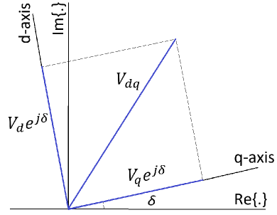
(a) The geometry of $dq$-components on the system’s complex plane.

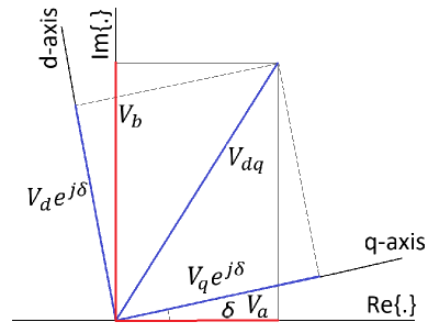
(b) The decomposition of $dq$-components in both the system and the machine reference frames.

Figure 1: Relative position of the machine reference frame with respect to the system reference frame [20].

Now, we express network equations (14) in each generator’s reference frame so as to obtain the general network relationships. By substituting (18) and (20) into (15) we get:

$$\begin{split}I_{q,i}=&\sum_{j=1}^{|\mathcal{N}|}\Big{[}V_{q,j}\Big{(}G_{ij}\cos(\eta_{ij})+B_{ij}\sin(\eta_{ij})\Big{)}\\ &+V_{d,j}\Big{(}G_{ij}\sin(\eta_{ij})-B_{ij}\cos(\eta_{ij})\Big{)}\Big{]}\\ I_{d,i}=&\sum_{j=1}^{|\mathcal{N}|}\Big{[}V_{q,j}\Big{(}-G_{ij}\sin(\eta_{ij})+B_{ij}\cos(\eta_{ij})\Big{)}\\ &+V_{d,j}\Big{(}G_{ij}\cos(\eta_{ij})+B_{ij}\sin(\eta_{ij})\Big{)}\Big{]}\end{split}$$ (21)

where, for ease of notation, angle differences are written as $\eta_{ij}=\delta_{i}-\delta_{j}$.

III FRAMEWORK FORMULATION

III-A Network Model

As discussed in Section II, the power network is represented by the nodal set of equations (10), which can be also written in the rectangular form (14). In order to formulate the network model, we separate the real and the imaginary part of equation (14) so as to form the following $(2\times|\mathcal{N}|)$-input/$(2\times|\mathcal{N}|)$-output system

$$\begin{bmatrix}I_{a}\\ I_{b}\end{bmatrix}=\begin{bmatrix}G_{n}&-B_{n}\\ B_{n}&G_{n}\end{bmatrix}\begin{bmatrix}V_{a}\\ V_{b}\end{bmatrix}\\ =H_{2n}\begin{bmatrix}V_{a}\\ V_{b}\end{bmatrix}=g^{N}([V_{a}^{\textrm{T}}\ V_{b}^{\textrm{T}}])$$ (22)

where $H_{2n}$ denotes the matrix relating the vectors $[V_{a}^{\textrm{T}}\ V_{b}^{\textrm{T}}]^{\textrm{T}}$ with the vectors $[I_{a}^{\textrm{T}}\ I_{b}^{\textrm{T}}]^{\textrm{T}}$. The vector function $g^{N}:\ \mathbb{R}^{2|\mathcal{N}|}\to\mathbb{R}^{2|\mathcal{N}|}$ provides an alternative notation so as to comply with the definitions that we are about to use in the forthcoming paragraphs. The aforementioned system is illustrated in Figure 2.

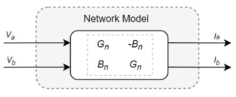
Figure 2: The $(2\times|\mathcal{N}|)$-input/$(2\times|\mathcal{N}|)$-output system that is used to model the power network.

We are now ready to examine the passivity properties that are revealed through the aforementioned modeling. Taking into account that Assumption 3 holds, we first provide the following fundamental passivity definition [23].

Definition 2

Consider the system described by the memory-less function $y=g(t,u)$ where $g:[0,\infty)\times\mathbb{R}^{p}\to\mathbb{R}^{p}$. This system is passive if $u^{\textrm{T}}y\geq 0$.

As stated above, the static network model (22) is passive if and only if the inequality within Definition 2 is satisfied, i.e.

$$u^{\textrm{T}}y=[V_{a}^{\textrm{T}}\ V_{b}^{\textrm{T}}]\begin{bmatrix}I_{a}\\ I_{b}\end{bmatrix}\geq 0$$ (23)

for all $V_{a}$, $V_{b}$, $I_{a}$, $I_{b}$ $\in{\color[rgb]{0,0,0}{\mathbb{R}^{|\mathcal{N}|}}}$.

Lemma 1

The network system defined in (22) with inputs the vectors of bus voltage components $[V_{a}^{\textrm{T}}\ V_{b}^{\textrm{T}}]^{\textrm{T}}$ and outputs the vectors of net injected current components $[I_{a}^{\textrm{T}}\ I_{b}^{\textrm{T}}]^{\textrm{T}}$ is passive.

Remark 2

We see within the proof of Lemma 1 (provided in the appendix) that condition (23) always holds and that the passivity of the network system is ensured regardless of its topology. Specifically, due to the form of the composite matrix $H_{2n}$, the positive semi-definiteness of the network’s conductance matrix $G_{n}$ is sufficient for condition (23) to be satisfied. $G_{n}$ in turn, is always positive semi-definite since it has positive diagonal elements and is diagonally dominant.

Remark 3

As we are about to discuss in the next section, the majority of the recent literature dealing with power system stability in general network topologies adopts lossless networks, i.e. $G_{n}=0$. The main reason for considering such simplification lies in the fact that when the analysis is carried out in $dq$-coordinates, the passivity property holds only for lossless networks. For the proposed approach, under such assumption condition (23) becomes

$$u^{\textrm{T}}y=[V_{a}^{\textrm{T}}\ V_{b}^{\textrm{T}}]\begin{bmatrix}0&-B_{n}\\ B_{n}&0\end{bmatrix}\begin{bmatrix}V_{a}\\ V_{b}\end{bmatrix}=0$$ (24)

Note that the network’s passivity follows here easily from the skew-symmetry of the matrix $H_{2n}$.

III-B Bus Dynamics

In order to incorporate the bus models and derive stability results for the interconnected system, both the network and the bus dynamics have to be expressed in the same reference frame, which is chosen here as the system reference frame. In contrast to the recent literature, we therefore transform the bus dynamics into the system reference frame instead of each bus local $dq$-coordinates, and consider that each of the $|\mathcal{N}|$ buses forms a 2-input/2-output system so as to fit with the network formulation described in the previous section. A graphical representation of the interconnected system is provided in Figure 3 where the multi-input/multi-output network system is connected to the aggregate bus dynamics. The bus models are expressed in the system reference frame by incorporating the mappings $T$ and $T^{-1}$ (equations (17)-(20)) into the bus dynamics. This approach is to the best of our knowledge novel, and allows the consideration of more relaxed conditions for the network while giving the opportunity for decentralized stability analysis and control.

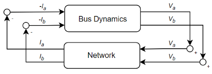
Figure 3: The power network represented as an interconnection of input/output systems associated with the bus dynamics and transmission lines, respectively.

We now introduce a broad class of systems that are used to represent the bus models. We consider that these dynamical systems have inputs the phasor components of the net current injection $(-I_{a,i},-I_{b,i})\in\mathbb{R}^{2}$, states $x_{i}\in X\subseteq\mathbb{R}^{k}$ and outputs the phasor components of the bus voltage $(V_{a,i},V_{b,i})\in\mathbb{R}^{2}$. The state-space representation of the aforementioned dynamical systems is given by:

$$\begin{split}\dot{x}_{i}=&f_{i}(x_{i},u_{i})\\ y_{i}=&g_{i}(x_{i},u_{i})\quad i\in\mathcal{N}\end{split}$$ (25)

where $u_{i}=[-I_{a,i},-I_{b,i}]$, $y_{i}=[V_{a,i},V_{b,i}]$. The vector functions $f_{i}:\mathbb{R}^{k_{i}}\times\mathbb{R}^{2}\to\mathbb{R}^{k_{i}}_{i}$ and $g_{i}:\mathbb{R}^{k_{i}}\times\mathbb{R}^{2}\to\mathbb{R}^{2}$ are locally Lipschitz for any $i\in\mathbb{N}$. We also note here that the bus dynamics (25) can be of arbitrary dimension.

We now describe what is meant by an equilibrium of the interconnected system (22) and (25).

Definition 3

The constant vector $\hat{x}=[\hat{x}_{1}\ \hat{x}_{2}\ \ldots\ \hat{x}_{|\mathcal{N}|}]$, $\hat{x}_{i}\in\mathbb{R}^{k_{i}}$ is an equilibrium of the interconnected system (22) and (25), if the time derivative of the states in (25) is equal to zero when $x_{i}=\hat{x}_{i},\ i\in\mathcal{N}.$

III-C Passivity Conditions on Bus Dynamics

We now present passivity conditions on the bus dynamics, which when satisfied guarantee the asymptotic stability of the equilibria of the interconnected system (22) and (25). We note here that these conditions are decentralized. Before presenting the aforementioned conditions, we first provide the following definition for input-strict passivity [23].

Definition 4

Consider a dynamical system represented by the state space model

$$\begin{split}\dot{x_{i}}=&f_{i}(x_{i},u_{i})\\ y_{i}=&g_{i}(x_{i},u_{i})\end{split}$$ (26)

where $f_{i}:\mathbb{R}^{n_{i}}\times\mathbb{R}^{p_{i}}\to\mathbb{R}^{n_{i}}$ and $g_{i}:\mathbb{R}^{n_{i}}\times\mathbb{R}^{p_{i}}\to{\color[rgb]{0,0,0}{\mathbb{R}^{p_{i}}}}$ are locally Lipschitz. Such system is said to be locally input strictly passive about the equilibrium $(\hat{u}_{i},\hat{x}_{i})$, if there exist open neighborhoods $U_{i}$ and $X_{i}$ about $\hat{u}_{i},\ \hat{x}_{i}$, respectively, a continuously differentiable function $\mathcal{V}_{i}(x_{i})$ (called the storage function), and a function $\phi(.)$ such that

$$(u_{i}-\hat{u}_{i})^{\textrm{T}}(y_{i}-\hat{y}_{i})\geq\dot{\mathcal{V}_{i}}+(u_{i}-\hat{u}_{i})^{\textrm{T}}\phi_{i}(u_{i}-\hat{u}_{i})$$ (27)

for all $u_{i}\in U_{i}$ and all $x_{i}\in X_{i}$, where $(u_{i}-\hat{u}_{i})^{\textrm{T}}\phi_{i}(u_{i}-\hat{u}_{i})>0$ for $u_{i}\neq\hat{u}_{i}$.

Remark 4

For linear systems or systems linearized about an equilibrium the passivity property can be easily verified by means of computationally efficient methods using the KYP lemma [24], or via the positive realness of the transfer function. We note here that the KYP lemma also allows to explicitly construct the storage function of the system, which for linear systems is a quadratic function of the form $\mathcal{V}(x_{i})=x_{i}^{\textrm{T}}P_{i}x_{i}$, where matrix $P_{i}\in\mathbb{R}^{n_{i}\times n_{i}}$ is obtained by solving a convex optimization problem (a semidefinite program). For nonlinear systems it can be verified by exploiting structural properties such as feedback interconnections of passive systems, or via an explicit construction of the storage function (see e.g. [16], [25]). An alternative way to check the passivity property for linear systems is via the positive realness of their transfer function $G(s)$. In particular, input strict passivity is implied if $G(j\omega)+G^{\textrm{T}}(-j\omega)$ is positive definite (or equivalently has positive eigenvalues) for all $\omega\in\mathbb{R}$.

In the assumptions below $\hat{x}$ is an equilibrium point of the interconnected system, and $(\hat{u}_{i},\hat{x}_{i})$ are the corresponding constant inputs and states of the bus dynamics (25) at this point.

Assumption 4

For each $i\in\mathcal{N}$, each of the bus dynamical systems (25) satisfies a local input-strict passivity property about $(\hat{u}_{i},\hat{x}_{i})$, in the sense described in Definition 4.

Similarly to the approach presented in [16], [26], we assume that the aforementioned passivity property holds without specifying the precise form of the bus dynamics. This will allow us to include in the stability analysis a broad class of bus dynamics and a variety of frequency and/or voltage control mechanisms.

Finally, to guarantee convergence, we will require two additional conditions on the behavior of the interconnected system (22) and (25). These conditions will be used in the proof of the convergence result in Theorem 1.

Assumption 5

Consider the dynamics (25) at bus $i$. When $u_{i}(t)=\hat{u}_{i}\ \forall t$, then $\hat{x}_{i}$ is asymptotically stable, i.e. there exists neighbourhood $\tilde{X}_{i}$ about $\hat{x}_{i}$ s.t. for all $x_{i}(0)\in\tilde{X}_{i}$, we have $x_{i}(t)\rightarrow\hat{x}_{i}$ as $t\rightarrow\infty$.

Remark 5

Note that this condition is trivially satisfied in many cases as generation dynamics are usually open loop stable. The condition could also be relaxed to allow for integrators at some buses (used in e.g, secondary control), but this is not done here for simplicity in the presentation.

Assumption 6

The storage functions $\mathcal{V}_{i}$ in Assumption 4 have a strict local minimum at the point $\hat{x_{i}}$.

Remark 6

This is a technical condition often satisfied. This is satisfied, for example, for any linear system if the latter is observable and controllable.

III-D Stability Result

The passivity properties presented for both the network and the bus model are now exploited in order to show that the equilibria of the system (22) and (25), for which the assumptions stated are satisfied, are asymptotically attracting. This is stated in the following theorem.

Theorem 1

Suppose there exists an equilibrium of the interconnected system (25), (22) for which the bus dynamics (25) satisfy Assumptions 4 - 6 for all $i\in\mathcal{N}$. Then this equilibrium is asymptotically stable, i.e. there exists an open neighbourhood $S$ about this point such that for all initial conditions $x(0)\in S$, the solutions of the system converge to this point.

Remark 7

It should be noted that the stability conditions in Theorem 1 are decentralized as they are conditions on the local bus dynamics. A distinctive feature of those is that the bus dynamics are formulated at the system reference frame, thus allowing to consider networks with losses as was discussed in Section III-A. In Section V it will be shown that these stability conditions are not conservative by applying those to real power networks with realistic data.

IV DISCUSSION

IV-A Network

As we mentioned before, the main difference between the proposed approach and the recent literature is that the analysis is carried out in the system reference-frame instead of each local machine reference-frame. It should be noted that even though this change of reference frame does not have an effect in a centralized stability analysis, it provides important benefits when stability is deduced by means of decentralized conditions. In particular, as it has been shown in the paper, a local passivity property at the bus dynamics in this reference frame is sufficient to deduce stability in a general network, without having to resort to a lossless assumption on the transmission lines. It should also be noted that both the active and the reactive power flows across the network are taken into account in the models and the bus voltage magnitudes are not considered to remain constant when sudden generation or load disturbances appear across the power grid.

In addition, the transformation into the system reference-frame leads to simpler network equations. Specifically, by comparing equations (15) with equations (21), it is easy to discern the complexity added when the analysis is carried out in the local machine reference-frame due to the existence of the sinusoids. This was the main reason why several simplifications were considered in the stability analysis for power networks within the recent literature. Such an important simplification was the adoption of lossless power networks where equations (21) are reduced to

$$\begin{split}I_{q,i}=&\sum_{j=1}^{|\mathcal{N}|}\Big{[}B_{ij}V_{q,j}\sin(\eta_{ij})-B_{ij}V_{d,j}\cos(\eta_{ij})\Big{]}\\ I_{d,i}=&\sum_{j=1}^{|\mathcal{N}|}\Big{[}B_{ij}V_{q,j}\cos(\eta_{ij})+B_{ij}V_{d,j}\sin(\eta_{ij})\Big{]}.\end{split}$$ (28)

Commonly, the previous equations are further simplified by assuming that $V_{d,i}=0\ \forall\ i\in\mathcal{N}$, which leads to the following simpler and less accurate form:

$$\small{I_{q,i}=\sum_{j=1}^{|\mathcal{N}|}\Big{[}B_{ij}V_{q,j}\sin(\eta_{ij})\Big{]}\mbox{ and }I_{d,i}=\sum_{j=1}^{|\mathcal{N}|}\Big{[}B_{ij}V_{q,j}\cos(\eta_{ij})\Big{]}}.$$ (29)

In order to avoid counting in the generator’s transient reactances and thus to facilitate the analysis, several works such as [27, 15, 28, 29] also considered that the $q$-axis bus voltage is equal to the $q$-axis transient emf, i.e. $V_{q,i}=E^{\prime}_{q,i}$ (see also section IV-B). inline,color=yellow!60, linecolor=orange!250]need to say what $E_{q,i}$ is, referring e.g. to the Machine models in the next section

IV-B Bus Dynamics

The adoption of a broad class of systems to represent bus dynamics provides another advantage of the proposed approach, since it allows to include dynamics associated with a variety of power system components such as generators, loads, inverter-based RES, and FACTS devices. It also gives the opportunity to use more accurate higher order dynamical models and incorporate voltage and frequency control mechanisms at the same time. Dynamic models of the synchronous generator are commonly used in power system stability studies, as their stable operation guarantees the security and the reliability of a power system. The adoption of more accurate generator models is hence crucial, since simpler ones can fail to accurately predict the behavior of the system [30].

We describe below the fourth-order generator model which is widely considered to be sufficiently accurate to analyze electromechanical dynamics, and present how this can be incorporated into our approach. The aforementioned model which will be also used to verify our results in Section V, is described by the following set of differential equations:

$$\begin{split}M_{i}\Delta\dot{\omega}_{i}=&P_{i}^{m}-P_{i}^{e}-D_{i}\Delta\omega_{i}\\ \dot{\delta}_{i}=&\Delta\omega_{i}\\ T^{\prime}_{do,i}\dot{E^{\prime}}_{q,i}=&E_{f,i}-E^{\prime}_{q,i}+I_{d,i}(X_{d,i}-X^{\prime}_{d,i})\\ T^{\prime}_{qo,i}\dot{E^{\prime}}_{d,i}=&-E^{\prime}_{d,i}-I_{q,i}(X_{q,i}-X^{\prime}_{q,i})\end{split}$$ (30)

where the electrical power $P_{i}^{e}=E^{\prime}_{q,i}I_{q,i}+E^{\prime}_{d,i}I_{d,i}+(X^{\prime}_{d,i}-X^{\prime}_{q,i})\ I_{d,i}\ I_{q,i}$. The synchronous generator described in (30), is modeled in its local $dq$-reference frame and it is represented by the transient emfs $E^{\prime}_{d,i}$ and $E^{\prime}_{q,i}$ behind the transient reactances $X^{\prime}_{d,i}$ and $X^{\prime}_{q,i}$ as defined by the following equation

$$\begin{bmatrix}V_{q,i}\\ V_{d,i}\end{bmatrix}=\begin{bmatrix}E^{\prime}_{q,i}\\ E^{\prime}_{d,i}\end{bmatrix}-\begin{bmatrix}R_{i}&-X^{\prime}_{d,i}\\ X^{\prime}_{q,i}&R_{i}\end{bmatrix}\begin{bmatrix}I_{q,i}\\ I_{d,i}\end{bmatrix}.$$ (31)

In particular, the synchronous generator model forms a 2-input/2-output system with inputs the currents $-I_{d,i}$ and $-I_{q,i}$, and outputs the voltages $V_{d,i}$ and $V_{q,i}$. In order to allow the coupling with the network model (22), the generator dynamics have to be transformed into the system reference frame. We therefore incorporate the mappings (17) - (20) into the synchronous generator dynamics, and the current $dq$-components $I_{d,i}$ and $I_{q,i}$ are replaced in equations (30) by the net injected current components $I_{a,i}$ and $I_{b,i}$ using (19). The outputs $V_{a,i}$ and $V_{b,i}$ are derived by (31) as follows

$$\begin{bmatrix}V_{a,i}\\ V_{b,i}\end{bmatrix}=T_{i}^{-1}\begin{bmatrix}E^{\prime}_{q,i}\\ E^{\prime}_{d,i}\end{bmatrix}-T_{i}^{-1}\begin{bmatrix}R_{i}&-X^{\prime}_{d,i}\\ X^{\prime}_{q,i}&R_{i}\end{bmatrix}T_{i}\begin{bmatrix}I_{a,i}\\ I_{b,i}\end{bmatrix}$$ (32)

TABLE I: Description of the Main Variables and Parameters appearing in the Synchronous Generator Models

Variables		Parameters
$\Delta\omega$	Frequency deviation	$M$	Moment of inertia
$\delta$	Stator’s phase angle	$D$	Damping coefficient
$E^{\prime}_{d}$	d-axis transient EMF	$X_{d}$	d-axis synchronous reactance
$E^{\prime}_{q}$	q-axis transient EMF	$X^{\prime}_{d}$	d-axis transient reactance
$I_{d}$	d-axis current	$T^{\prime}_{d}$	d-axis open-circuit time constant
$I_{q}$	q-axis current	$X_{q}$	q-axis synchronous reactance
$V_{d}$	d-axis bus voltage	$X^{\prime}_{q}$	q-axis transient reactance
$V_{q}$	q-axis bus voltage	$T^{\prime}_{q}$	q-axis open-circuit time constant
$P^{m}$	Mechanical power	$R_{i}$	stator windings resistance
$P^{e}$	Electrical power
$E_{f}$	exciter output emf
$E_{g}$	controlled voltage

We can now identify that the aforementioned generator model matches to the class of bus models (25). The dynamic model of the generator corresponds to the vector function $f_{i}$ while equations (32) match to the vector functions $g_{i}$. The presented formulation still holds for the second and the third-order synchronous generator models, where the transient emfs $E^{\prime}_{d,i}$ and $E^{\prime}_{q,i}$, respectively, are assumed to remain constant. Higher order models, such as the fifth or the sixth order models can be also incorporated in this framework in an analogous way. In these models, the synchronous generators are represented by their subtransient emfs $E^{{}^{\prime\prime}}_{d,i}$ and $E^{{}^{\prime\prime}}_{q,i}$ behind the subtransient reactances $X^{{}^{\prime\prime}}_{d,i}$ and $X^{{}^{\prime\prime}}_{q,i}$. More detailed information about generator modeling can be found in [18, 19, 21].

As we discussed earlier, the generator dynamics can be expanded further so as to introduce the dynamics of frequency and/or voltage control mechanisms, thus allowing the derivation of more accurate stability results. Such frequency and voltage control mechanisms include several types of turbine governors, exciters and power system stabilizers. A graphical representation of the adaption of a synchronous generator model to the proposed framework along with the incorporation of frequency and voltage control is provided in Figure 4. We highlight here the fact that the passivity conditions which ensure the asymptotic stability of the equilibria, refer to the bus dynamics and not specifically to the voltage and the frequency control systems that are applied. This allows us to include more advanced regulation mechanisms which in most cases are not passive (e.g. turbine governors, excitation systems etc.). This is an important advantage since such dynamics are often omitted in approaches commonly presented in the related literature, due to the additional complexity they introduce.

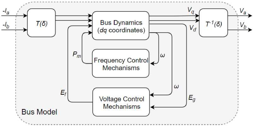
Figure 4: A graphical representation of a generator model expressed in system reference frame.

Finally, it should be noted that loads, inverter-based RES and FACTS devices can also easily be incorporated within our approach. However, an explicit analysis of such models is beyond the scope of the current paper and is therefore omitted. Several detailed dynamic models for the aforementioned power system components can be found within [18, 31, 22, 32, 33, 34, 35]. It is crucial to mention here that the framework becomes more flexible and easy to apply when we deal with bus dynamics that do not involve a rotating axis. In such cases, bus dynamics are already expressed in the system reference frame and thus there is no need to include the maps $T_{i}$ and $T_{i}^{-1}$ into the adopted dynamics.

V SIMULATIONS

In this section we verify our framework and the derived stability results through applications on the Two Area Kundur Test System [18] and the IEEE New York / New England 68-bus interconnection system [36]. These applications focus on generator buses and are carried out using the Power System Toolbox (PST) [37]. Within the simulations, the generators are modeled by the fourth-order dynamics (30) on which both frequency and voltage control mechanisms are applied. Specifically, frequency and voltage control are carried out by turbine governors and exciters respectively, while PSSs are applied to the generator’s excitation system. The adopted models of the turbine governors, the exciters and the PSSs can be found in PST manual [37].

In order to facilitate the verification of the passivity property on the generator buses of the test systems, we linearize the dynamics of each generator bus individually about an equilibrium. The equilibria are identified by solving a Power Flow problem for each test system respectively. In order to verify the passivity of the bus models we use Linear Matrix Inequalities (LMIs) whose application on passivity verification is extensively described in [25, Section 2]. An alternative way to verify the passivity of bus dynamics with transfer matrix $G_{i}(s)$, is by checking the positive definiteness of the matrix $G_{i}(\textrm{j}\omega)+G_{i}^{\textrm{T}}(-\textrm{j}\omega)$ as indicated in [38]. In particular, the positive definiteness is ensured when the eigenvalues of the matrix are positive.

We first deal with the Four Machine Two-Areas Kundur Test System which is widely used for stability studies. The passivity of the four generator buses is verified using LMIs, for the following four different cases: (i) no turbine governor / no exciter / no PSS, (ii) turbine governor / no exciter / no PSS, (iii) turbine governor / exciter / no PSS and (iv) turbine governor / exciter / PSS. All generator buses are not passive when neither of the available control mechanisms is employed. When turbine governors are added to generators, bus dynamics are slightly damped but they still remain non passive. The exciters further passivate the generator buses making buses 1 and 2 passive. Buses 11 and 12 still remain non passive. Finally, the application of PSSs to the generators completely passivates the dynamics.

The proposed approach is also applied on the generator buses of the IEEE 68 bus test system. According to the derived results, the generator buses are also non passive for the cases (i) and (ii). In both cases, the power system collapses after a sudden change of load across the network. On the other hand, when the excitation system is applied to the generators, the generator buses are considerably damped and, although the system presents an oscillatory behavior, it remains stable when a generation-load mismatch occurs. To be more specific, the application of the excitation system on the grid-connected generators makes generator buses 53, 59, 61 and 64 passive while the rest remain non passive. Finally, the incorporation of the PSSs at the generator exciters passivates further the generator buses, and results in a more stable and robust operation. All generator buses are now passive except from buses 58, 62, 63 and 65. However, we can achieve to passivate these generator buses by slightly increasing the transient reactances $X^{\prime}_{d}$ and $X^{\prime}_{q}$ of the respective generators (approximately $15\%$). These results are illustrated in Figures 5 and 6 which present the frequency and the voltage deviation at bus 27 respectively, when a sudden change of 1pu is applied at the load buses 1, 9 and 18. This change corresponds to a total change of 300 MW. We should note here that the IEEE 68 bus test system consists of a total load of 18.33 GW. Due to the fact that the system collapses when the excitation system is not applied to the generators, we omit the respective figures for the cases (i) and (ii). We should also note here that, although not all the generator buses are passive, the power system is stable. From these results, it becomes clear that under a proper design of the control mechanisms which are applied to the generators, we can achieve to completely passivate the generator buses of the network, and thus to ensure the asymptotic stability of the power system.

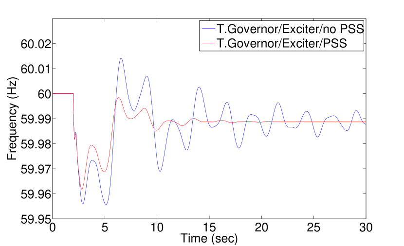
Figure 5: Frequency deviation at bus 27 after a sudden change of 1pu at the load buses 1, 9 and 18.

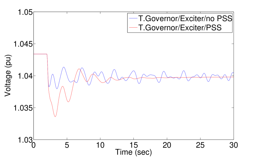
Figure 6: Voltage deviation at bus 27 after a sudden change of 1pu at the load buses 1, 9 and 18.

In order to demonstrate how existing control mechanisms can be designed so as to satisfy the passivity property, we consider a generator bus with turbine governor where the bus dynamics are non passive without excitation control, and also a simple first order exciter leads to marginally non passive dynamics. We then discuss how modifing the exciter by adding an additional phase lag compensator can passivate the dynamics.

In particular, the modified exciter has transfer function given by

$$E_{f,i}=\frac{K_{a}}{1+sT_{a}}\frac{1+sT_{c}}{1+sT_{b}}E_{g,i}$$ (33)

where the term $(1+sT_{c})/(1+sT_{b})$ is the phase lag compensator that has been added such that the passivity property is satisfied. We describe below in detail how the parameters of the transfer function in (33) have been chosen and provide their values in Table II below.

TABLE II: Values of the constants of the modified exciters.

Generator	$\bm{K_{a}}$	$\bm{T_{a}}$	$\bm{T_{b}}$	$\bm{T_{c}}$
53	20	0.05	3.3	0.3
54	20	0.05	1.5	0.1
55	20	0.05	2.5	0.2
56	20	0.05	1.5	0.5
57	20	0.05	1.7	0.3
58	20	0.05	1.4	0.7
59	20	0.05	1.5	0.4
60	20	0.05	1.8	0.2
61	20	0.05	1.9	0.1
62	20	0.05	1.8	0.4
63	20	0.05	1.0	0.1
$64^{**}$	20	0.05	0.0	0.0
$65^{**}$	20	0.05	0.0	0.0
$66^{**}$	20	0.05	0.0	0.0
$67^{**}$	20	0.05	0.0	0.0
$68^{**}$	20	0.05	0.0	0.0
** : No modifications were applied to the generator.

The gain $K_{a}$ is the dc gain of the exciter and the parameter $T_{a}$ determines the cutoff frequency (given by $1/T_{a}$) of the first order system $1/(1+sT_{a})$. Very large values of $K_{a}$ and $1/T_{a}$ will violate the passivity of the bus dynamics and lead to oscillatory responses. On the other hand, small values of $K_{a}$ and $1/T_{a}$ will lead to a feedback scheme that is slow in its response. Therefore $K_{a}$ and $1/T_{a}$ are chosen large enough while also ensuring that the passivity property is not violated.

The selection of the values of the time constants $T_{b}$ and $T_{c}$ of the phase lag compensator is carried out so that a reduction in gain is achieved in the problematic frequency range where the passivity property is violated, i.e. the range of frequencies where the eigenvalues of $G(j\omega)+G^{T}(-j\omega)$ are negative, where $G(s)$ is the transfer matrix of the corresponding bus dynamics. The phase lag compensator is therefore designed such that $1/T_{b}$ is smaller than the problematic frequencies. Parameter $T_{c}$ is then chosen such that $T_{c}<T_{b}$ with $T_{c}$ sufficiently small so as to achieve a sufficient reduction in gain, and also $1/T_{c}<1/T_{a}$ so as to avoid additional phase lag at higher frequencies.

This process is demonstrated in Figure 7 where the eigenvalues of the matrix $G(j\omega)+G^{\textrm{T}}(-j\omega)$ are illustrated at different frequencies, where $G(s)$ is the transfer function of the linearized dynamics (25) at generator bus 53. The figure shows the eigenvalues in the regime where the passivity property is violated. In particular, as seen from the figure the passivity property is violated in the frequency range $\omega\in[0.3,3]$ rads/sec (since the eigenvalues are negative) when no exciter or the simple first order exciter are used. The figure also shows that the addition of an appropriately tuned phase lag compensator passivates the dynamics. It should be noted that the essence of this design process is that it is decentralized, based on only the local bus dynamics, without requiring at each bus to be aware of the dynamics of the entire network as in a classical small signal analysis.

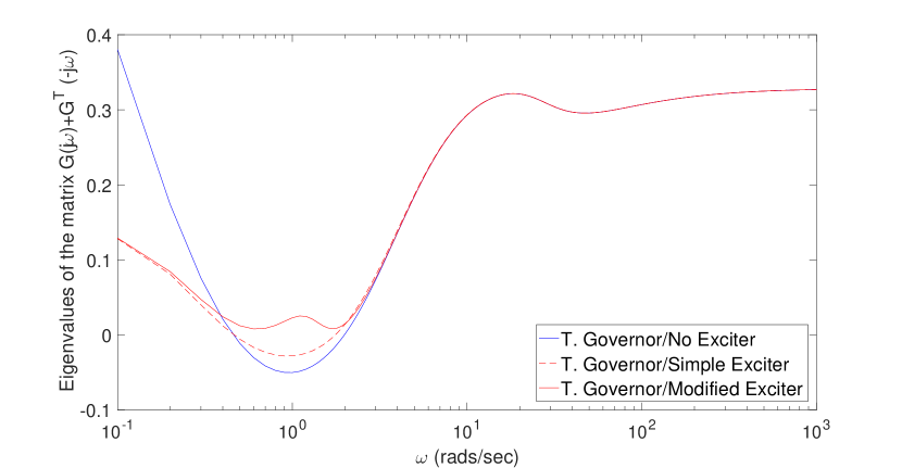
Figure 7: Eigenvalues of $G(j\omega)+G^{\textrm{T}}(-j\omega)$, where $G(s)$ is the transfer function of the linearized dynamics (25) at generator bus 53. The figure shows the eigenvalues in the problematic range where the passivity property is violated.

The performance of the system when the passivity based design described above is applied at all buses within the network is illustrated in Figures 8 and 9. The figures present the frequency and the voltage deviation, respectively, at bus 27, when a sudden change of 3pu is applied at the load buses 1, 9, 18, 20, 37 and 42. As it can be seen from both the aforementioned figures, the introduction of an appropriately tuned lag compensator to the excitation system of the generator results in a significantly less oscillatory behavior of the system. We should note here that for the dynamic simulation, we considered a total load change of $1800$ MW which correspond to $10\%$ of the grid-connected load.

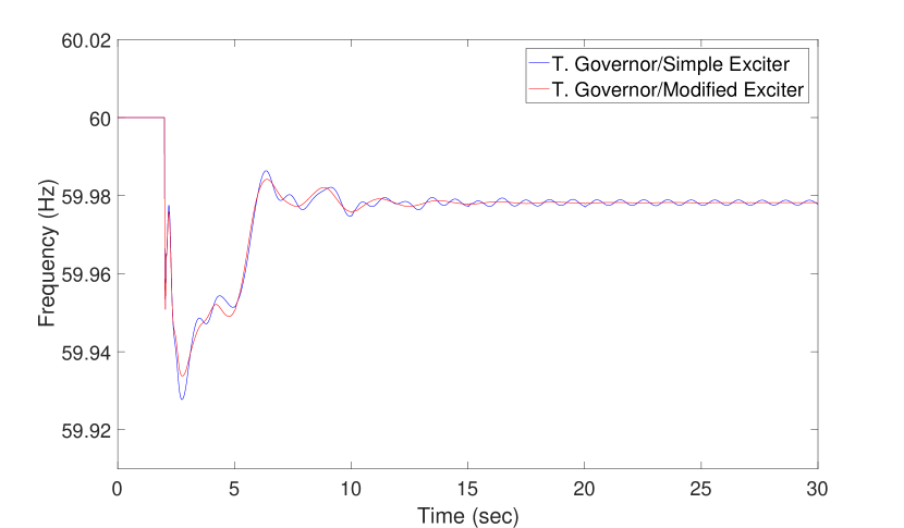
Figure 8: Frequency deviation at bus 27 after a sudden change of 3pu at the load buses 1, 9, 18, 20, 37 and 42.

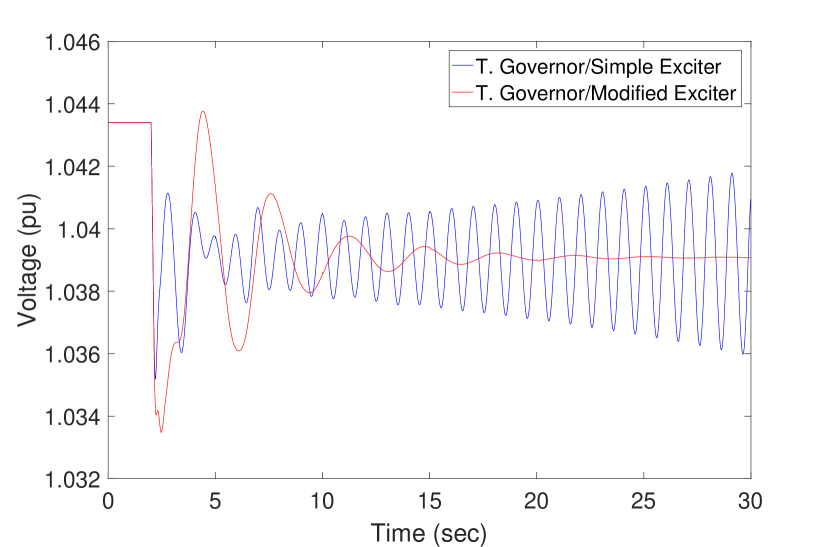
Figure 9: Voltage deviation at bus 27 after a sudden change of 3pu at the load buses 1, 9, 18, 20, 37 and 42.

The stability enhancement achieved through the modification of the initial simple exciter is also illustrated through the eigenanalysis of the test system. As it can be seen from Figure 10, the application of a lag compensator to the exciter that passivates the bus dynamics significantly damps the calculated modes. More specifically, when the simple exciter that violates the passivity property is employed to the generators the system is small-signal unstable since there exists an eigenvalue with positive real part. On the other hand, the application of the modified exciter on the generators stabilizes the system moving all the eigenvalues to the left half plane. Moreover, the proposed compensator to the excitation system of the generators yields a good damping ratio for the modes of the system.

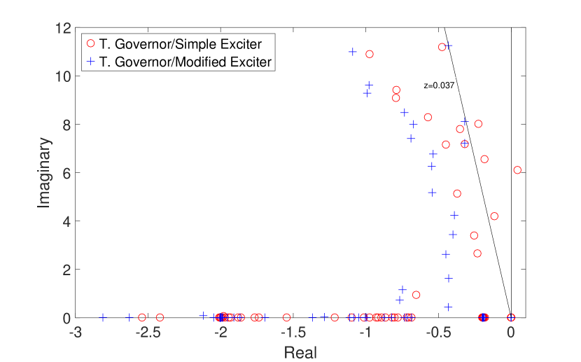
Figure 10: Eigenvalues of the linearized network dynamics of the IEEE 68 bus test system.

VI CONCLUSIONS

Within the paper, we have presented a novel passivity-based approach for decentralized stability analysis and control of power grids through the transformation of both the network and the bus dynamics into the system reference frame. In particular, by adopting an input/output formulation, the power networks were shown to constitute a passive system even if the network’s lossy nature is taken into account. We have then introduced a broad class of bus dynamics that fits to the aforementioned network formulation and provided passivity conditions which when satisfied, guarantee the asymptotic stability of the entire power system in a decentralized manner. Furthermore, we discussed the opportunities and advantages offered by this approach while explaining how the proposed framework can allow the inclusion of various power system components, such as synchronous generators and dynamic loads. Finally, our approach has been verified through various applications in the Two Area Kundur and the IEEE 68 bus test systems.

APPENDIX

Proof of Lemma 1

By substituting the network equations (22) in inequality (23) we get

$$\small{\begin{split}u^{\textrm{T}}y=&[V_{a}^{\textrm{T}}\ V_{b}^{\textrm{T}}]H_{2n}\begin{bmatrix}V_{a}\\ V_{b}\end{bmatrix}=[V_{a}^{\textrm{T}}\ V_{b}^{\textrm{T}}]\begin{bmatrix}G_{n}&-B_{n}\\ B_{n}&G_{n}\end{bmatrix}\begin{bmatrix}V_{a}\\ V_{b}\end{bmatrix}\\ =&V_{a}^{\textrm{T}}G_{n}V_{a}+V_{b}^{\textrm{T}}G_{n}V_{b}\geq 0\end{split}}$$ (34)

for all $V_{a}$, $V_{b}$ $\in{\color[rgb]{0,0,0}{\mathbb{R}^{|\mathcal{N}|}}}$. The inequality (34) reveals that the passivity of the network is ensured when the composite matrix $H_{2n}$ or equivalently its diagonal elements $G_{n}$, are positive semidefinite matrices.

$G_{n}\in\mathbb{R}^{|\mathcal{N}|\times|\mathcal{N}|}$ is a square, sparse symmetric matrix with non negative diagonal and negative off-diagonal elements, i.e., $G_{ii}\geq 0$ and $G_{ij}\leq 0$ $\forall\ i,\ j=1,2,\dots,|\mathcal{N}|$. It is also diagonally dominant as the following equation holds:

$$\small{G_{ii}=-\sum_{j\neq i}^{|\mathcal{N}|}G_{ij}\Rightarrow|G_{ii}|=\sum_{j\neq i}^{|\mathcal{N}|}|G_{ij}|}\quad(i,j)\in\mathcal{E}$$ (35)

In order to prove the positive semidefiniteness of the matrix $G_{n}$, we now define the Geshgorin discs $D_{i}(G_{ii},R_{i}),\ i=1,2,\dots,|\mathcal{N}|$. $D_{i}$ is a closed disc centered at $(G_{ii},0)$, with radius $R_{i}=\sum_{i\neq j}|G_{ij}|$. As stated above the matrix $G_{n}$ has positive diagonal elements and is also diagonally dominant. Subsequently, its Geshgorin discs lie in the right half plane, have center on the real axis and are tangent to the imaginary axis since $G_{ii}-R_{i}=0,\ \forall\ i=1,2,\dots,|\mathcal{N}|$. According to the Geshgorin circle theorem [39], the eigenvalues of the matrix $G_{n}$ lie within its Geshgorin discs, corresponding to its columns (or equivalently to its rows). Subsequently, $G_{n}$ has eigenvalues with non negative real parts which immediately leads to the fact that it is positive semidefinite [39]. Condition (23) is therefore satisfied. $\square$

Proof of Theorem 1

We will use the dynamics (25) and (22) together with Assumptions 4-6 to prove Theorem 1. In particular, it will be shown that the storage functions that follow from the passivity property can be used to construct a Lyapunov function for the network, with stability then deduced using Lasalle’s theorem.

Since the passivity conditions for the bus dynamics are considered about the equilibrium point, we define the deviations from the corresponding equilibrium values $\hat{I}_{a},\hat{I}_{b},\hat{x},\hat{V}_{a},\hat{V}_{b}$ as $\tilde{I}_{a,i}=I_{a,i}-\hat{I}_{a,i},\ \tilde{I}_{b,i}=I_{b,i}-\hat{I}_{b,i},\ \tilde{x}_{i}=x_{i}-\hat{x}_{i},\ \tilde{V}_{a,i}=V_{a,i}-\hat{V}_{a,i},\ \tilde{V}_{b,i}=V_{b,i}-\hat{V}_{b,i}$ for the net current injection components, the states and the bus voltage components respectively.

We now consider the following candidate Lyapunov function for the closed-loop system (22) and (25) $\mathcal{V}(x)=\sum_{i=1}^{|\mathcal{N}|}\mathcal{V}_{i}(x_{i})$, where $\mathcal{V}_{i}(x_{i})$ is the storage function of the bus dynamics with input $u_{i}=[-\tilde{I}_{a,i},-\tilde{I}_{b,i}]$ and output $y_{i}=[\tilde{V}_{a,i},\tilde{V}_{b,i}]$. Considering the passivity conditions described in Assumption 4, we calculate the derivative of the above Lyapunov function with respect to time. In particular, we get

$$\small{\begin{split}\dot{\mathcal{V}}=&\sum_{i=1}^{|\mathcal{N}|}{\color[rgb]{0,0,0}{\dot{\mathcal{V}}_{i}}}\leq\sum_{i=1}^{|\mathcal{N}|}\Big{(}[-\tilde{I}_{a,i}\ -\tilde{I}_{b,i}]\ \begin{bmatrix}\tilde{V}_{a,i}\\ \tilde{V}_{b,i}\end{bmatrix}-\phi_{i}(-\tilde{I}_{a,i},-\tilde{I}_{b,i})\Big{)}\\ =&-[\tilde{V}_{a}^{\textrm{T}}\ \tilde{V}_{b}^{\textrm{T}}]H_{2n}\begin{bmatrix}\tilde{V}_{a}\\ \tilde{V}_{b}\end{bmatrix}-\sum_{i=1}^{|\mathcal{N}|}\phi_{i}(-\tilde{I}_{a,i},-\tilde{I}_{b,i})\end{split}}$$ (36)

whenever $(\tilde{V}_{a,i},\tilde{V}_{b,i})\in U_{i}$ and $\tilde{x}_{i}\in X_{i}$ for all $i\in\mathcal{N}$. Since the matrix $H_{2n}$ and the scalar valued functions $\phi_{i}$ are positive semidefinite and positive definite respectively, the inequality (36) becomes $\dot{\mathcal{V}}\leq 0$. We then make use of LaSalle’s theorem to prove the asymptotic convergence of the system’s trajectories to the equilibrium point. According to Assumption 6, the candidate Lyapunov function $\mathcal{V}$ has a strict local minimum at the equilibrium $\hat{x}$. Therefore for a sufficiently small $\epsilon>0$ there exists a compact positively invariant set $\Xi:=\{x:{\mathcal{V}(x)-\mathcal{V}(\hat{x})}\leq\epsilon,\ \hat{x}\in\Xi,\ \Xi\ \text{connected}\}$ that lies in the neighborhoods stated in the assumptions. Lasalle’s Invariance Principle can now be applied with the function $\mathcal{V}$ on the compact positively invariant set $\Xi$. This guarantees that all solutions of the interconnected system (25) and (22) with initial conditions $x(0)\in\Xi$ converge to the largest invariant set within $\Upsilon:=\Xi\cap\{x:\dot{\mathcal{V}}=0\}$. From the positive definiteness of function $\phi$ we have that $\dot{\mathcal{V}}=0$ implies that $\tilde{I}_{a,i}=\tilde{I}_{b,i}=0$, i.e. $I_{a,i}=\hat{I}_{a,i}$, $I_{b,i}=\hat{I}_{b,i}$. Hence from Assumption 5 we have that the only invariant set in $\Upsilon$ is the equilibrium point $x(t)=\hat{x}$. Therefore, for any initial condition $x(0)\in\Xi$ we have convergence to the equilibrium point, which completes the proof. $\square$

References

- [1] P. Kundur, J. Paserba, V. Ajjarapu, G. Andersson, A. Bose, C. Canizares, N. Hatziargyriou, D. Hill, A. Stankovic, C. Taylor, et al., “Definition and classification of power system stability IEEE/CIGRE joint task force on stability terms and definitions,” IEEE Transactions on Power Systems, vol. 19, no. 3, pp. 1387–1401, 2004.
- [2] O. Ma, N. Alkadi, P. Cappers, P. Denholm, J. Dudley, S. Goli, M. Hummon, S. Kiliccote, J. MacDonald, N. Matson, et al., “Demand response for ancillary services,” IEEE Transactions on Smart Grid, vol. 4, no. 4, pp. 1988–1995, 2013.
- [3] B. Kirby and E. Hirst, Ancillary service details: Voltage control. Oak Ridge National Laboratory, 1997.
- [4] H. Miyagi and A. Bergen, “Stability studies of multimachine power systems with the effects of automatic voltage regulators,” IEEE Transactions on Automatic Control, vol. 31, no. 3, pp. 210–215, 1986.
- [5] A. J. van der Schaft and B. M. Maschke, “Port-Hamiltonian systems on graphs,” SIAM Journal on Control and Optimization, vol. 51, no. 2, pp. 906–937, 2013.
- [6] B. Maschke, R. Ortega, and A. J. Van Der Schaft, “Energy-based lyapunov functions for forced hamiltonian systems with dissipation,” IEEE Transactions on Automatic Control, vol. 45, no. 8, pp. 1498–1502, 2000.
- [7] Y. Wang, D. Cheng, C. Li, and Y. Ge, “Dissipative hamiltonian realization and energy-based l 2-disturbance attenuation control of multimachine power systems,” IEEE Transactions on Automatic Control, vol. 48, no. 8, pp. 1428–1433, 2003.
- [8] S. Fiaz, D. Zonetti, R. Ortega, J. Scherpen, and A. Van der Schaft, “A port-hamiltonian approach to power network modeling and analysis,” European Journal of Control, vol. 19, no. 6, pp. 477–485, 2013.
- [9] T. Stegink, C. De Persis, and A. van der Schaft, “A unifying energy-based approach to stability of power grids with market dynamics,” IEEE Transactions on Automatic Control, vol. 62, no. 6, pp. 2612–2622, 2017.
- [10] J. Schiffer, E. Fridman, R. Ortega, and J. Raisch, “Stability of a class of delayed port-hamiltonian systems with application to microgrids with distributed rotational and electronic generation,” Automatica, vol. 74, pp. 71–79, 2016.
- [11] J. Schiffer, R. Ortega, A. Astolfi, J. Raisch, and T. Sezi, “Conditions for stability of droop-controlled inverter-based microgrids,” Automatica, vol. 50, no. 10, pp. 2457–2469, 2014.
- [12] S. Y. Caliskan and P. Tabuada, “Compositional transient stability analysis of multimachine power networks,” IEEE Transactions on Control of Network Systems, vol. 1, no. 1, pp. 4–14, 2014.
- [13] T. Stegink, C. De Persis, and A. van der Schaft, “Optimal power dispatch in networks of high-dimensional models of synchronous machines,” in 55th Conference on Decision and Control (CDC), pp. 4110–4115, IEEE, 2016.
- [14] M. Andreasson, R. Wiget, D. V. Dimarogonas, K. H. Johansson, and G. Andersson, “Distributed primary frequency control through multi-terminal hvdc transmission systems,” in American Control Conference (ACC), pp. 5029–5034, IEEE, 2015.
- [15] S. Trip, M. Bürger, and C. De Persis, “An internal model approach to (optimal) frequency regulation in power grids with time-varying voltages,” Automatica, vol. 64, pp. 240–253, 2016.
- [16] A. Kasis, E. Devane, C. Spanias, and I. Lestas, “Primary frequency regulation with load-side participation Part I: stability and optimality,” IEEE Transactions on Power Systems, vol. 32, no. 5, pp. 3505–3518, 2017.
- [17] J. D. Glover, M. S. Sarma, and T. Overbye, Power System Analysis & Design, SI Version. Cengage Learning, 2012.
- [18] P. Kundur, N. J. Balu, and M. G. Lauby, Power system stability and control, vol. 7. McGraw-Hill, 1994.
- [19] J. Machowski, J. Bialek, and J. Bumby, Power system dynamics: stability and control. J. Wiley & Sons, 2011.
- [20] A. R. Bergen and V. Vittal, Power systems analysis. Prentice Hall, 2000.
- [21] P. W. Sauer and M. Pai, “Power system dynamics and stability,” Urbana, vol. 51, 1997.
- [22] J. Schiffer, D. Zonetti, R. Ortega, A. M. Stanković, T. Sezi, and J. Raisch, “A survey on modeling of microgrids: From fundamental physics to phasors and voltage sources,” Automatica, vol. 74, pp. 135–150, 2016.
- [23] H. K. Khalil, Nonlinear Systems. Prentice Hall, 3rd ed., 2002.
- [24] N. Kottenstette, M. J. McCourt, M. Xia, V. Gupta, and P. J. Antsaklis, “On relationships among passivity, positive realness, and dissipativity in linear systems,” Automatica, vol. 50, no. 4, pp. 1003–1016, 2014.
- [25] M. J. McCourt and P. J. Antsaklis, “Demonstrating passivity and dissipativity using computational methods,” ISIS, p. 008, 2013.
- [26] E. Devane, A. Kasis, M. Antoniou, and I. Lestas, “Primary frequency regulation with load-side participation Part II: beyond passivity approaches,” IEEE Transactions on Power Systems, vol. 32, no. 5, pp. 3519–3528, 2017.
- [27] A. Kasis, E. Devane, and I. Lestas, “On the stability and optimality of primary frequency regulation with load-side participation,” in 54th Conference on Decision and Control (CDC), pp. 2621–2626, IEEE, 2015.
- [28] C. Zhao, U. Topcu, N. Li, and S. Low, “Design and stability of load-side primary frequency control in power systems,” IEEE Transactions on Automatic Control, vol. 59, no. 5, pp. 1177–1189, 2014.
- [29] J. Machowski, S. Robak, J. Bialek, J. Bumby, and N. Abi-Samra, “Decentralized stability-enhancing control of synchronous generator,” IEEE Transactions on Power Systems, vol. 15, no. 4, pp. 1336–1344, 2000.
- [30] E. Venezian and G. Weiss, “A warning about the use of reduced models of synchronous generators,” in International Conference on the Science of Electrical Engineering (ICSEE), pp. 1–5, IEEE, 2016.
- [31] I. Hiskens and J. Milanovic, “Load modelling in studies of power system damping,” IEEE Transactions on Power Systems, vol. 10, no. 4, pp. 1781–1788, 1995.
- [32] R. Teodorescu, M. Liserre, and P. Rodriguez, Grid converters for photovoltaic and wind power systems, vol. 29. J. Wiley & Sons, 2011.
- [33] H. Wang and F. Swift, “A unified model for the analysis of facts devices in damping power system oscillations. i. single-machine infinite-bus power systems,” IEEE Transactions on Power Delivery, vol. 12, no. 2, pp. 941–946, 1997.
- [34] H. Wang, F. Swift, and M. Li, “A unified model for the analysis of facts devices in damping power system oscillations. ii. multi-machine power systems,” IEEE Transactions on Power Delivery, vol. 13, no. 4, pp. 1355–1362, 1998.
- [35] H. Wang, “A unified model for the analysis of facts devices in damping power system oscillations. iii. unified power flow controller,” IEEE Transactions on Power Delivery, vol. 15, no. 3, pp. 978–983, 2000.
- [36] G. Rogers, Power system oscillations. Springer Science & Business Media, 2012.
- [37] J. Chow, G. Rogers, and K. Cheung, “Power system toolbox,” Cherry Tree Scientific Software,[Online] Available: http://www. ecse. rpi. edu/pst/PST. html, vol. 48, p. 53, 2000.
- [38] N. Kottenstette and P. J. Antsaklis, “Relationships between positive real, passive dissipative, & positive systems,” in American Control Conference (ACC), pp. 409–416, IEEE, 2010.
- [39] R. A. Horn and C. R. Johnson, Matrix analysis. Cambridge university press, 2012.