Electron-phonon cooling power in Anderson insulators

Abstract

We present a microscopic theory for electron-phonon energy exchange in Anderson insulators at low temperatures. The major contribution to the cooling power $J_{e-ph}(T_{el})$ as a function of electron temperature $T_{el}$ is shown to be directly related to the correlation function of the local density of electron states $K(\omega)$. In Anderson insulators not far from localization transition, correlation function $K(\omega)$ is enhanced at small $\omega$ by wavefunction’s multifractality and by the presence of Mott’s resonant pairs of states. The theory we develop explains a huge enhancement of the cooling power observed in insulating Indium Oxide films as compared to predictions of the theory previously developed for disordered metals.

I Introduction.

Energy exchange between electrons and phonons is crucial to many physical properties of Anderson insulators at low temperatures: it determines relatively slow rate of thermal equilibration. Surprizingly, no theory of such processes seems to be availalble. On the contrary, theory of electron-phonon inelastic coupling in disordered metals is known for a very long time pippard ; akhiezer ; schmid .

Experimentally, one of the most sensitive method to study electron-phonon cooling rate is based on the results of Ref.shahar ; Ovadia-Sacepe-Shahar where striking jumps by several orders of magnitude in current-voltage characteristics were observed at low temperatures in insulating Indium Oxide films. Similar effects were also observed in other insulating systems sanquer ; baturina . These jumps in resistance are the signatures of thermal bi-stability at weak electron-phonon coupling which can be analyzed using the balance between the Joule heat production and the electron cooling power  AKLA , and the temperature dependence of electron-phonon cooling rate can be experimentally obtained  Ovadia-Sacepe-Shahar . The out-cooling rate at low temperatures of electron system $T=T_{{\rm el}}$ appeared to be $J(T)=A\,T^{\beta}$, where $\beta\approx 6$ agreed well with the theory of electron-phonon cooling presented in AKLA .

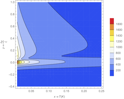
Figure 1: Enhancement factor for the cooling rate in the Anderson insulator ($y>0$) compared to the dirty metal ($y<0)$ as a function of temperature and proximity to the Anderson localization transition at $n=n_{c}$ (parametrized by the ratio of the Fermi wavelength $\lambda_{F}$ and the localization ($\xi>0$) or correlation ($\xi<0$) length, with $|\xi|/\lambda_{F}\sim(1-n/n_{c})^{-\nu}$, $\nu\approx 1.6$). Notice a persistent character of enhancement in insulator at low temperatures even far from the Anderson transition $\lambda_{F}/\xi=0$. This enhancement is caused by the pairs of Mott’s resonant states with multifractal structure inside localization volume, while the enhancement close to the Anderson transition both in metal and in insulator is caused by multifractality alone.

The problem with this result is that the experimentally observed pre-factor $A$ is 2-3 orders of magnitude larger than the one predicted by the theory of electron-phonon cooling in strongly disordered metals employed in AKLA . At first glance it is also strange that in an insulator the temperature dependence of the cooling is a power-law, while the temperature dependence of resistance is exponential or stretch exponential. However, the most surprising fact is that the theory of electron-phonon cooling in Anderson insulators is essentially missing, despite so much effort invested in studying hopping conductivity.

In this paper we present the theory of electron-phonon cooling in insulators at proximity to the Anderson localization transition when the momentum relaxation rate $\ell$ is of the order of the Fermi wavelength $\lambda_{F}=2\pi/k_{F}$, and the effects of multifractality CueKrav ; MFSC are significant. We show that the temperature dependence of the cooling rate at low temperatures is indeed a power-law, since the energy exchange between electron and phonon systems is local and does not involve electron transport in space. Therefore it is natural that the additional factor characterizing electron cooling in Anderson insulators obtained in this paper is given by the properly normalized correlation function $K(\omega)$ of the local density of states. This correlation function is enhanced due to multifractality of electron wave functions CueKrav ; MFSC , which results in an increasing cooling rate both in metals and in insulators close to the Anderson transition (see Fig.1). Another mechanism of enhancement of the cooling rate (also described by the same correlation function $K(\omega)$) is typical to insulators and is related with the Mott’s pairs of resonant states. It is similar to the logarithmic enhancement of the frequency-dependent conductivity in Anderson insulator Mott ; Berezinskii and efficient at low temperatures. It is because of this effect, enhanced by multifractality, that the enhancement factor shown in Fig.1 is drastically asymmetric on both sides of the Anderson transition.

At the values of the parameters typical to amorphous Indium Oxide films used in Ref.shahar ; Ovadia-Sacepe-Shahar , the total enhancement factor may be as large as 500-800 in the range of electron temperatures $20-100\,mK$ and it decreases very slowly as the system is driven deeper into the insulating phase (see Fig1). Moreover, the temperature dependence of the enhancement factor is logarithmic, which makes the effective power $\beta$ in the out-cooling rate only slightly modified compared to the case of dirty metal fn1 . This makes our theory a very plausible explanation of enhancement of the pre-factor $A$ in the cooling rate in the experiments Ovadia-Sacepe-Shahar .

However, the results of this paper are much more general. They are based on universal properties of random electron wave functions in the multifractal insulator CueKrav ; MFSC and are independent of a particular system as well of the presence or absence of superconductivity in it.

The paper is organized as follows. In Sec.II we present a general expression for the out-cooling rate in terms if exact electron wave functions in the presence of strong disorder. In Sec.III and Appendix B we show that the simple random-phase approximation for electron wave functions employed in the theory of Sec.II reproduces all the known results for the electron-phonon cooling obtained earlier using the impurity diagrammatic technique. In Sec.III we modify this random-phase approximation by introducing a non-trivial envelope of oscillating wave functions which accounts for the effects of multifractality and localization.The main result of this section is that the cooling rate is determined by the local density of states correlation function $K(\omega)$. In Sec.IV we review known properties of function $K(\omega)$, in particular the signatures of multifractality and the effect of Mott’s resonant pair on it. In Sections V and VI we compute the enhancement factor for the cooling rate due to these effects for the transverse and longitudinal phonons, respectively. In Conclusion we formulate the main results of the paper and discuss their implications for low-temperature experiments in Anderson insulators close to localization transitions.

II General expression for the cooling rate.

The out-cooling rate $J(T)$ is expressed Shtyk in terms of the phonon attenuation rate $\tau_{\rm ph}^{-1}$ due to electron phonon interaction:

$$J(T)=\int_{0}^{\infty}d\omega\,\omega\,\nu_{ph}(\omega)\,\frac{B_{ph}(\omega)}{\tau_{ph}(\omega)},$$ (1)

where $B_{\rm ph}(\omega)=\frac{1}{2}(\coth(\omega/2T)-1)$ is the phonon energy distribution function, and $\nu_{\rm ph}=\omega^{2}/(2\pi^{2}v_{s}^{3})$ is the 3d phonon density of states. The phonon attenuation rate and the sound velocity are different for transverse (t) and longitudinal (l) modes, and the total cooling rate $J_{{\rm tot}}(T)=J_{{\rm l}}(T)+2J_{{\rm t}}(T)$, each of the contributions being described by (1) with the corresponding $\tau_{ph}^{(t,l)}$ and sound velocities $v_{s}^{(t,l)}$.

Thus the primary object of interest is the phonon attenuation rate:

$$\frac{1}{\tau_{ph}}=\frac{1}{2\rho_{i}\,\omega}\,\mathop{\rm Im}(\Sigma_{\omega}^{R}-\Sigma_{\omega}^{A}),$$ (2)

where $\rho_{i}$ is the lattice mass density, and $\Sigma^{R(A)}=\hat{{\cal D}}\,\Pi^{R(A)}_{RPA}\,\hat{{\cal D}}$ is the (retarded or advanced) phonon self energy, given by a proper action of the gradient vertex operators $\hat{{\cal D}}$ on the RPA polarization bubble $\Pi^{R(A)}_{RPA}$.

In order to take the localized nature of electron wave functions into account we express the phonon attenuation rate in terms of the exact electron eigenfunctions $\psi_{n}({\bf r})$ and eigenvalues $E_{n}$. To this end we use the reference frame moving locally together with the lattice schmid ; Shtyk . In this frame the electron-phonon Hamiltonian takes the form Shtyk :

$$H_{{\rm e-ph}}=-\sum_{{\bf p},{\bf q}}p_{\alpha}\,(v_{\beta}\nabla_{\beta}\,u_{\alpha})_{{\bf q}}\,\Psi^{\dagger}_{{\bf p}}\Psi_{{\bf(p+q)}}$$

$$=\frac{1}{m}\int d^{d}{\bf r}\,[\nabla_{\beta}\,u_{\alpha}({\bf r})]\,\partial_{\alpha}\partial^{\prime}_{\beta}\;\Psi^{\dagger}(\bf r)\,\Psi({\bf r^{\prime}})|_{{\bf r}={\bf r^{\prime}}},$$ (3)

where $p_{\alpha}=-i\nabla_{\alpha}$, $v_{\beta}=p_{\beta}/m$ is the electron velocity operator, $\Psi_{{\bf p}}$ and $\Psi_{{\bf p+q}}$ are Fourier components of the Fermionic operators $\Psi^{\dagger}({\bf r})$ and $\Psi({\bf r^{\prime}})$, $m$ is the electron mass and $u_{\alpha}$ is the phonon-induced local shift of the lattice in the laboratory frame. The Greek symbols $\alpha,\beta$ in Eq.(II) and throughout the paper are the components of 3D vectors, the summation over repeated indexes being assumed. This Hamiltonian should be supplemented by the standard electron interaction with an impurity potential and the electron kinetic energy. The advantage of the co-moving frame is that the cross-terms with electron- phonon-impurity interaction do not appear, which makes calculations much simpler.

This interaction is screened by Coulomb interaction $V$. In the RPA approximation the screened phonon self-energy is given by:

$$\Sigma=\hat{{\cal D}}\Pi\hat{{\cal D}}+\hat{{\cal D}}\Pi\;\frac{V}{1-\Pi V}\;\Pi\hat{{\cal D}},$$ (4)

where

$$\hat{{\cal D}}\Pi=\frac{1}{m}\,[\nabla_{\beta}\,u_{\alpha}({\bf r})]\,\partial_{\alpha}\partial^{\prime}_{\beta}\,\Pi({\bf r},{\bf r^{\prime}};{\bf r}_{1},{\bf r^{\prime}}_{1})|_{{\bf r}={\bf r^{\prime}},{\bf r}_{1}={\bf r}_{1}^{\prime}},$$ (5)

$$\Pi\hat{{\cal D}}=\frac{1}{m}\,[\nabla_{\gamma}\,u_{\delta}({\bf r}_{1})]\,\partial_{1,\gamma}\partial^{\prime}_{1,\delta}\,\Pi({\bf r},{\bf r^{\prime}};{\bf r}_{1},{\bf r^{\prime}}_{1})|_{{\bf r}={\bf r^{\prime}},{\bf r}_{1}={\bf r}_{1}^{\prime}},$$ (6)

and $\Pi$ is the bare polarization bubble in which all effects of disorder are included but interaction is not.

Note that in the second term in Eq.(4) the fast momenta corresponding to the left vertex of the leftmost $\Pi$ is completely decoupled from the fast momenta corresponding to the right vertex of the rightmost $\Pi$. As the result the second term in Eq.(4) is proportional to $k_{F}^{4}\,\delta_{\alpha\beta}\,\delta_{\gamma\delta}$ and thus its contribution vanishes for transverse phonons. This is not the case for the first term in Eq.(4) at distances $|{\bf r}-{\bf r}_{1}|<\ell$, where $\ell$ is the mean free path.

In what follows we first consider the effect of the first term in Eq.(4). Using (4),(II) and (2) one can express the corresponding contribution to $\tau_{ph}$ as follows (see Appendix for details of derivation):

$$\frac{1}{\tau_{{\rm ph}}^{(1)}}=\pi\,\frac{q_{\beta}q_{\delta}}{m^{2}}\,e_{\alpha}e_{\gamma}\,\frac{1}{\rho_{i}}\,\int d^{d}{\bf R}\,e^{i{\bf q}{\bf R}}\,K_{\alpha\beta\gamma\delta}({\bf R},\omega),$$ (7)

where $e_{\alpha}$ is the $\alpha$ component the unit vector of phonon polarization, $q_{\alpha}$ is the component of the phonon wave vector ${\bf q}$ with $|{\bf q}|=q=\omega/v_{s}$, ${\cal V}$ is the volume, and the function $K_{\alpha\beta\gamma\delta}({\bf R};\omega)$ is defined as

$$K_{\alpha\beta\gamma\delta}({\bf R};\omega)=\left\langle\sum_{nm}(\partial_{\alpha}\psi^{*}_{m}({\bf r}))\,(\partial_{\beta}\psi_{n}({\bf r}))\,(\partial_{\gamma}\psi^{*}_{n}({\bf r^{\prime}}))\,(\partial_{\delta}\psi_{m}({\bf r^{\prime}}))\,\delta(E-E_{n})\,\delta(E^{\prime}-E_{m})\right\rangle.$$ (8)

In (8) we denote disorder averaging by $\langle.\rangle$. After such an averaging $K_{\alpha\beta\gamma\delta}({\bf R},\varepsilon)$ becomes a function of ${\bf r}-{\bf r^{\prime}}={\bf R}$ and $E-E^{\prime}=\varepsilon$ in the bulk of a sample and the spectrum.

III Effects of localization and multifractality.

To further proceed we employ the following ansatz for the electron wave functions:

$$\psi_{n}({\bf r})=\int\frac{d\Omega_{{\bf s}}}{4\pi}\,a^{(n)}_{{\bf s}}({\bf r})\,e^{ik_{F}\,{\bf s}\,{\bf r}},$$ (9)

where $|{\bf s}|=1$ and $a_{{\bf s}}^{(n)}({\bf r})$ is a Gaussian random variable with zero mean and the correlation function:

$$\langle a^{(n)}_{{\bf s}}({\bf r})\,a^{(m)}_{{\bf s^{\prime}}}({\bf r^{\prime}})\rangle=\delta_{nm}\,\delta_{{\bf s},{\bf s^{\prime}}}\,e^{-\frac{|{\bf r}-{\bf r^{\prime}}|}{2\ell}}\;\phi_{n}({\bf r})\phi_{m}({\bf r^{\prime}}).$$ (10)

Eqs.(9),(10) are essentially a generalization of the semi-classical Berry’ ansatz Berry for the case of localization and multifractality. The exponential factor with the momentum relaxation length $\ell$ in Eq.(10) accounts for the fast randomization of wave-function phases due to elastic scattering, while positive functions $\phi_{n}({\bf r})$ describe normalized (and smooth at a scale $\ell$ )   envelopes of the wave functions, averaged over fast de Broglie oscillations:

$$[\phi_{n}({\bf r})]^{2}=\overline{\psi_{n}^{2}({\bf r})}\;{\cal V}.$$ (11)

Such an envelopes $\phi_{n}({\bf r})$ are equal to 1 in the semi-classical Berry’s approximation $k_{F}\ell\gg 1$ when both localization and multifractality effects are absent and wave functions are ergodic. At $k_{F}\ell\sim 1$ when multifractality and/or localization is present, these envelope functions have a non-trivial shape which depends on the index $n$ and on the realization of disorder. Thus the averaging in (10) is incomplete. It involves only the random phase averaging and assumes subsequent disorder averaging of the amplitude. Possibility to separate nearly universal fast wave-functions oscillations from the slow envelope that contains information about multifractal behavior was discussed in a different way in Ref. MirlinFyodorov1997 . This idea has been successfully exploited in Ref.RRG in numerical computation of the multifractal spectrum $f(\alpha)$ in order to sort out the effect of nodes which dominates distribution of small eigenfunction amplitudes.

It is shown in the Appendix A, that plugging (9) and (10) with $\phi_{n}({\bf r})=1$ in (7) one exactly reproduces at $q\ell\ll 1$ an expression for $\tau_{{\rm ph}}^{(t)}$ obtained earlier for diffusive metals schmid ; Reyzer ; KrYud :

$$\frac{1}{\tau_{{\rm ph}}^{(t)}}=\frac{q^{2}\,k_{F}^{4}\ell}{30\pi^{2}\,\rho_{i}}=\frac{q^{2}}{10}\frac{k_{F}\ell}{\rho_{i}}\,n_{{\rm e}},$$ (12)

where $n_{{\rm e}}$ is the total (two-spin) electron density. The corresponding result for $J_{t}(T)$ is:

$$J_{t}(T)=\frac{4\pi^{4}}{630}\frac{(k_{F}\ell)n_{{\rm e}}}{\rho_{i}\,[v_{s}^{(t)}]^{5}}\,T^{6}.$$ (13)

Taking now into account $\phi_{n}({\bf r})\neq 1$ in (10) one obtains for (8),(7),(9) the following expression for $\tau^{(1)}_{{\rm ph}}$:

$$\frac{1}{\tau^{(1)}_{{\rm ph}}}=\pi\,\nu_{0}^{2}\,k_{F}^{4}\,\frac{q_{\beta}q_{\delta}}{m^{2}\rho_{i}}\,e_{\alpha}e_{\gamma}\,\int d^{3}{\bf R}\,e^{i{\bf q}{\bf R}}\,e^{-|{\bf R}|/\ell}\int\frac{d\Omega_{{\bf s}}}{4\pi}\int\frac{d\Omega_{{\bf s^{\prime}}}}{4\pi}\,s_{\alpha}s_{\delta}s^{\prime}_{\beta}s^{\prime}_{\gamma}\,e^{-ik_{F}\,({\bf s}-{\bf s^{\prime}}){\bf R}}\,K(\omega;{\bf R}),$$ (14)

where $\nu_{0}$ is the mean density of states at the Fermi level, $\Delta=(\nu_{0}{\cal V})^{-1}$ is the mean level spacing in an entire volume ${\cal V}$ and $K(\omega;{\bf R})=\Delta^{2}\left\langle\sum_{n,m}\phi_{n}({\bf r})\,\phi_{m}({\bf r^{\prime}})\,\phi_{m}({\bf r})\,\phi_{n}({\bf r^{\prime}})\;\delta(E-E_{n})\delta(E+\omega-E_{m})\right\rangle$. As the exponential factor $e^{-|{\bf R}|/\ell}$ makes the main domain of integration over ${\bf R}$ in (14) to be $|{\bf R}|\lesssim\ell$ and because of the smooth behavior of the envelope functions $\phi_{n}({\bf r})$ at such scale, one can replace $K(\omega;{\bf R})\rightarrow K(\omega,0)\equiv K(\omega)$. Then after angular integration over unit vectors ${\bf s},{\bf s^{\prime}}$ and integration over $R$ in (14), one obtains in the limit $|{\bf q}|\ell\ll 1$:

$$\frac{1}{\tau^{(1)}_{{\rm ph}}}=\frac{2\pi^{2}}{15}\frac{\nu_{0}^{2}k_{F}^{2}\ell}{m^{2}\,\rho_{i}}\,(3q_{||}^{2}+q_{\perp}^{2})\;K(\omega),$$ (15)

where $q_{||}$ and $q_{\perp}$ are the longitudinal and the transverse components of the phonon wave vector and

$$K(\omega)=\Delta^{2}\left\langle\sum_{n,m}\phi_{n}^{2}({\bf r})\,\phi^{2}_{m}({\bf r^{\prime}})\;\delta(E-E_{n})\delta(E+\omega-E_{m})\right\rangle$$ (16)

is the local density-of-states correlation function studied in Refs. CueKrav ; MFSC .

For transverse phonons ($q_{||}=0$) Eq.(15) gives the total phonon attenuation rate. It is proportional to the properly normalized electron local density of states correlation function $K(\omega)$ which is course-grained at a scale $\ell$. All the effects of localization and/or multifractality are encoded in this correlation function, while the effects of fast randomization of wave function phases by impurity scattering are taken into account by averaging over momentum directions $\mathbf{s},\mathbf{s^{\prime}}$ in Eq.(14).

Equations (15),(16) are the main result of our paper. Strictly speaking it is valid in $2+\epsilon$ ($\epsilon\ll 1$) dimensions where the scale separation $k_{F}\gg\ell^{-1}\gg\xi^{-1}$ holds even in insulator close to the Anderson transition where the localization length $\xi$ is large. As customary, we extend this result (with the accuracy up to a factor of order 1) for 3D samples and thick films with $k_{F}\ell\sim 1$.

IV The function $K(\omega)$ close to localization transition.

The behavior of the correlation function $K(\omega)$ was studied in detail in Ref.CueKrav ; MFSC . It was shown that for $E_{0}\gg\omega\gg\delta_{\xi}$, where $\delta_{\xi}=(\nu_{0}\xi^{3})^{-1}$ is the level spacing in the volume characterized by the correlation/localization length $\xi$, and $E_{0}$ is of the order of total bandwidth of conduction band, the effects of multifractality lead to the power-law enhancement of $K(\omega)=(E_{0}/\omega)^{\gamma}$, where $\gamma=1-d_{2}/3\approx 0.59$ is determined by the fractal dimension $d_{2}\approx 1.24\pm 0.03$ Roemer . This effect is due to the non-ergodicity of wave functions which do not occupy all the available volume causing the enhancement of their amplitude by normalization. Furthermore, the support sets of different wave functions are strongly correlated thus giving rise to enhancement of the overlap function $K(\omega)$. Albeit analysis in CueKrav concerned the case of non-interacting electrons, the subsequent study KrAminiMull has shown that localization transition and multifractality survive almost unchanged when Coulomb interaction is taken into account.

As $\omega$ decreases below $\delta_{\xi}$ the behavior of $K(\omega)$ starts to depend on whether the system is insulating or metallic. In the latter case $K(\omega)\sim(E_{0}/\delta_{\xi})^{\gamma}$ saturates at its value for $\omega=\delta_{\xi}$. However, in the insulator $K(\omega)\sim(E_{0}/\delta_{\xi})^{\gamma}\,\ln^{d-1}(\delta_{\xi}/\omega)$ increases further upon $\omega$ decrease CueKrav ; MFSC . This logarithmic enhancement is due to the Mott’s pairs of resonant levels which results in a well known Mott ; Berezinskii logarithmic enhancement of frequency-dependent conductivity $\sigma(\omega)\sim\omega^{2}\,\ln^{d+1}(\omega)$ in insulator. The difference in the power of logarithm in $K(\omega)$ and $\sigma(\omega)$ is due to the square of the dipole moment matrix element entering the conductivity. Both limiting cases in a 3D insulator can be combined in one interpolating expression MFSC :

$$K(\omega)=\frac{(E_{0}/\delta_{\xi})^{\gamma}\,\ln^{2}(\delta_{\xi}/\omega)}{c+(\omega/\delta_{\xi})^{\gamma}\,\ln^{2}(\delta_{\xi}/\omega)},\;\;\;\;(c\sim 1).$$ (17)

V Enhancement of cooling in a weak insulator.

Because of the strong dependence of the cooling power $J\propto v_{s}^{-5}$ on the sound velocity $v_{s}$, the cooling is usually dominated by the transverse phonons which sound velocity is typically smaller by a factor of about 2. Then neglecting the contribution of longitudinal phonons to cooling one obtains from (1):

$$J_{t}(T_{{\rm el}})=\frac{8}{5\pi^{2}}\frac{(k_{F}\ell)\,n_{{\rm e}}}{\rho_{i}\,[v_{s}^{(t)}]^{5}}\,T_{{\rm el}}^{6}\,R(T_{{\rm el}}),$$ (18)

where $T_{{\rm el}}$ is the temperature of electron system and the function

$$R(T)=\int_{0}^{\infty}dx\,x^{5}\,(\coth(x)-1)\,K(2T\,x).$$ (19)

Actually the integral in (19) is strongly peaked at $2x\approx 5$, thus the ratio $J(T_{el})/T^{6}_{el}$ is proportional to $K(5T_{el})$. In a limited interval of electron system temperatures $T_{{\rm el}}=10-100\,mK$ the enhancement factor $R(T_{{\rm el}})$ for typical parameters of Indium Oxide films $E_{0}=1000\,K$, $\delta_{\xi}=10\,K$, $c=1$ is well approximated by the power law $R(T)\approx\left(T_{0}/T_{\rm el}\right)^{0.55}$ with $T_{0}\approx 1700\,K$, see Fig.2. Thus the effective power of temperature in $J(T_{{\rm el}})$ should be $\beta_{{\rm eff}}\approx 5.5$ rather than 6.0, in agreement with Ref.Sacepe2018 . The overall enhancement factor for this values of parameters varies from 700 to 200 at $T_{{\rm el}}=10\,mK-100\,mK$ which is consistent with experiment Ovadia-Sacepe-Shahar . The dependence of the $R(T)$ factor on the local level spacing $\delta_{\xi}$ is rather weak, see inset to Fig.2.

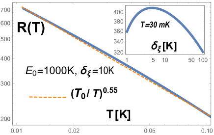
Figure 2: Enhancement factor $R(T)$ in Eqs. (18),(20) as a function of temperature for $E_{0}=1000\,K$ and $\delta_{\xi}=10\,K$. The dashed line represents a power law $(T_{0}/T)^{0.55}$ with $T_{0}=1710\,K$. Both the value of $R(T)$ and the exponent in the apparent power-law dependence are in agreement with experiment Refs.Ovadia-Sacepe-Shahar ; Sacepe2018 . In the inset: the enhancement factor $R$ as a function of $\delta_{\xi}$ for $T_{{\rm el}}=30\,mK$, $E_{0}=1000\,K$.

VI Cooling by longitudinal phonons.

Considering the contribution of longitudinal phonons to cooling rate, one has to take into account screening given by the second term in Eq.(4). The simplest case is the universal limit of screening when $V(q)\Pi\gg 1$ which is always the case in a 3D metal in the limit $q\rightarrow 0$ due to long-ranged Coulomb interaction $V(q)\propto 1/q^{2}$. In Anderson insulator this limit is approximate controlled by the large value of the dielectric constant close to the localization transition IvanovCuevasFeigelman . In this limit the electro-neutrality condition is strictly enforced and the second term in Eq.(4) takes the universal form $-(\hat{{\cal D}}\Pi)\;\Pi^{-1}\;(\Pi\hat{{\cal D}})$. One can approximate $\hat{{\cal D}}\Pi\approx\frac{\nabla{\bf u}}{m}\,k_{F}^{2}\,\delta_{\alpha\beta}\,\Pi$, and $\Pi\hat{{\cal D}}\approx\frac{\nabla{\bf u}}{m}\,k_{F}^{2}\,\delta_{\gamma\delta}\,\Pi$. Now proceeding in the same way as above using (9),(10) and taking into account also the longitudinal part of (15) we obtain the contribution of the longitudinal phonons to electron cooling:

$$J_{l}(T_{{\rm el}})=\frac{24}{5\pi^{2}}\frac{(k_{F}\ell)\,n_{{\rm e}}}{\rho_{i}\,[v_{s}^{(l)}]^{5}}\,T_{{\rm el}}^{6}\,R(T_{{\rm el}}).$$ (20)

As in Eq.(18), this result differs only by a factor $R(T_{{\rm el}})$ from that for a disordered metal schmid ; Reyzer .

Note that the above method of calculation using the ansatz (10) is valid only for local contributions, as it completely ignores a possibility of building a density-density propagator, the ’diffuson’. However, in the universal limit of screening the diffuson cannot be excited, as it is forbidden by electro-neutrality. The effect of incomplete screening on the longitudinal phonon decay rate and cooling is much more involved ( see e.g. Ref. Shtyk ). It may play some role in low-dimensional cases where the effects of incomplete Coulomb screening are stronger.

VII Conclusions.

The main result of this paper is given by Eqs.(15,16) which relates phonon decay rate $1/\tau(\omega)$ due to inelastic interaction with electrons, and correlation function of the local density of states $K(\omega)$ characterizing electron wave-functions near Anderson mobility edge. A direct consequence of this relation is a strong enhancement of the electron-phonon cooling power in weak insulators, in comparison with usual diffusive metals, as demonstrated by Eqs.(18,19) and Figs.1,2. For the case of insulating Indium-Oxide films, studied in Ref.Ovadia-Sacepe-Shahar , this enhancement is estimated to be in the range of 500-1000, in agreement with the experimental data. In general, our results suggest that measurements of the cooling rate Eq.(18) or ultrasound attenuation rate Eq.(15) provide a direct access to the electronic local density of states (LDoS) correlation function $K(\omega)$.

On a more technical side, we expect that the same relation (15) can be obtained by means of functional ”sigma-model” approach like the one developed in KamGlaz .

The above results are general and valid for any 3D Anderson insulator with long localization length and relatively weak Coulomb interaction (slight modification of our formulas will also work for 2D Anderson insulators). In particular, one can use this approach to analyze the data on bistability of I-V characteristics and switching between high-resistance and low-resistance branches as function of applied voltage, as reported for a number of various semiconductors or insulators, see Refs. 1 ; 2 ; 3 ; 4 . However, one should keep in mind that in insulators with strong Coulomb interaction it might be difficult to disentangle Coulomb correlation effects from purely localization effects. In such a case effective correlation function $K_{\rm eff}(\omega)$ may differ from its non-interacting version given in Eq.(17).

Our results for the electron-phonon cooling power make it possible to establish conditions for the observation of many-body localization transition in electronic insulators, predicted theoretically more than decade ago BAA but did not yet observed. One of the crucial problems to be solved in this respect is to find an insulator with an extremely low thermal coupling between electrons and phonons, yet with measurable electric conductance. Our theory will be instrumental to solve this important issue.

The behavior of the cooling power very similar to our prediction has been recently seen in the resistive state of moderately disordered superconducting Indium Oxide films at strong magnetic field and low temperatures: see Sec. IV of the Supplementary Information to Ref. Sacepe2018 , where $J(T_{\rm el})\propto T_{{\rm el}}^{5.5}$ was observed. An enhancement (compared to the prediction for dirty metals with $k_{F}\ell\sim 0.3$) by a factor 400-800 of cooling power per carrier in insulating $Nb_{x}Si_{1-x}$ can also be extracted from the results of Ref.NbSi .

Finally, we note that the obtained results are not expected to hold for pseudo-gaped insulators where single-electron DoS is strongly suppressed due to local pairing MFSC . Indeed, electron-phonon cooling rate in insulating state of Indium-Oxide realized at relatively low magnetic field is known Sacepe-personal to be much lower (and follow much faster temperature dependence) than the high-field data reported in Ref. Ovadia-Sacepe-Shahar . The reason for that difference is that strong magnetic field (above approximately 10 Tesla) destroys local pairs and makes electron spectrum gapless.

VIII Acknowledgments.

We are grateful to Claire Marrache, Benjamin Sacepe, Zvi Ovadyahu and Dan Shahar for numerous discussions of experimental data. This research was partially supported by the Skoltech NGP grant. V.E.K. is grateful to M. A. Skvortsov for illuminating discussions and hospitality at Skoltech where the major part of this work was done. M.V.F appreciates hospitality of Abdus Salam ICTP where the final part of this work was done.

Appendices

Appendix A General expression for phonon attenuation rate in terms of electron wave functions.

In order to take the localized nature of electron wave functions into account we express the phonon attenuation rate in terms of the exact electron eigenfunctions $\psi_{n}({\bf r})$ and eigenvalues $E_{n}$. Using (2)-(3) of the main text one can express the contribution to $\tau_{ph}$ from the first term of (4) as follows:

$$\frac{1}{\tau_{{\rm ph}}^{(1)}}=\frac{\pi}{2}\,\frac{q_{\beta}q_{\delta}}{m^{2}}\,e_{\alpha}e_{\gamma}\,\frac{1}{\rho_{i}\omega}\,\frac{1}{{\cal V}}\int dE\int dE^{\prime}\int d^{d}{\bf r}\int d^{d}{\bf r^{\prime}}\,e^{i{\bf q}({\bf r}-{\bf r^{\prime}})}\,F_{E,E^{\prime}}(\omega)\,K_{\alpha\beta\gamma\delta}({\bf r},{\bf r^{\prime}};E,E^{\prime}),$$ (21)

where $e_{\alpha}$ is the $\alpha$ component the unit vector of phonon polarization, $q_{\alpha}$ is the component of the phonon wave vector ${\bf q}$ with $|{\bf q}|=q=\omega/v_{s}$, ${\cal V}$ is the volume, $F_{EE^{\prime}}(\omega)=\left[\tanh\left(\frac{E^{\prime}+\omega}{2T}\right)-\tanh\left(\frac{E^{\prime}}{2T}\right)\right]\,\delta(E^{\prime}-E+\omega)$ is the Fermi distribution factor and the function $K_{\alpha\beta\gamma\delta}({\bf r},{\bf r^{\prime}};E,E^{\prime})$ is defined as

$$K_{\alpha\beta\gamma\delta}({\bf r},{\bf r^{\prime}};E,E^{\prime})=\left\langle\sum_{nm}(\partial_{\alpha}\psi^{*}_{m}({\bf r}))\,(\partial_{\beta}\psi_{n}({\bf r}))\,(\partial_{\gamma}\psi^{*}_{n}({\bf r^{\prime}}))\,(\partial_{\delta}\psi_{m}({\bf r^{\prime}}))\,\delta(E-E_{n})\,\delta(E^{\prime}-E_{m})\right\rangle.$$ (22)

In (22) we denote disorder averaging by $\langle.\rangle$. After such an averaging $K_{\alpha\beta\gamma\delta}({\bf r},{\bf r^{\prime}};E,E^{\prime})=K_{\alpha\beta\gamma\delta}({\bf R},\varepsilon)$ becomes a function of ${\bf r}-{\bf r^{\prime}}={\bf R}$ and $E-E^{\prime}=\varepsilon$ in the bulk of the spectrum. One can use the (approximate) translation invariance in the energy space and perform integration over $E^{\prime}$:

$$\int dE^{\prime}\,F_{E,E^{\prime}}(\omega)=2\omega\,\delta(\varepsilon-\omega).$$ (23)

Now the general expression for $\tau_{ph}^{(1)}$ takes the following form:

$$\frac{1}{\tau_{{\rm ph}}^{(1)}}=\pi\,\frac{q_{\beta}q_{\delta}}{m^{2}}\,e_{\alpha}e_{\gamma}\,\frac{1}{\rho_{i}}\,\int d^{d}{\bf R}\,e^{i{\bf q}{\bf R}}\,K_{\alpha\beta\gamma\delta}({\bf R},\omega),$$ (24)

Appendix B Phonon attenuation rate in disordered metals.

At $k_{F}\ell\gg 1$ when the effects of multifractality can be neglected the correlation function $K(\omega)\approx 1$ at $\omega\gg\Delta$. Here we consider this limit in order to show that our approach based on Eq.(11),(12) of the main text (in which $\phi_{n}(r)=1$) reproduces the well known results of Refs. [15,16] where the diagrammatic approach was adopted.

We start by evaluating the angular integrals over unit vectors ${\bf s}$ and ${\bf s^{\prime}}$ in Eq.(14) of the main text. The result should have the following form:

$$I_{1}\,\delta_{\alpha\delta}\delta_{\beta\gamma}+I_{2}\,(\delta_{\alpha\beta}\delta_{\gamma\delta}+\delta_{\alpha\gamma}\delta_{\beta\delta}),$$ (25)

as the integrals do not contain any preferential direction.

The quantities $I_{1}$ and $I_{2}$ can be found from the following equations:

$$9I_{1}+6I_{2} = \int d^{3}{\bf R}\,e^{-R/\ell}\,\left|\int\frac{d\Omega_{{\bf s}}}{4\pi}\,e^{ik_{F}{\bf s}{\bf R}}\,\right|^{2},$$ (26)

$$3I_{1}+12I_{2} = \int d^{3}{\bf R}\,e^{-R/\ell}\,\int\frac{d\Omega_{{\bf s}}}{4\pi}\int\frac{d\Omega_{{\bf s^{\prime}}}}{4\pi}\,e^{ik_{F}({\bf s}-{\bf s^{\prime}}){\bf R}}\,({\bf s}{\bf s}^{\prime})^{2}.$$ (27)

The integral under the absolute value sign in Eq.(26) is nothing but the Friedel oscillation in 3D space:

$$\Psi_{{\rm Fried}}=\left(\frac{\sin(k_{F}R)}{k_{F}R}\right).$$ (28)

Thus the R.H.S. of Eq.(26) reduces to:

$$\int d^{3}{\bf R}\,\left(\frac{\sin(k_{F}R)}{k_{F}R}\right)^{2}e^{-R/\ell}=\frac{8\pi\,\ell^{3}}{1+4(k_{F}\ell)^{2}}.$$ (29)

The double angular integral in Eq.(27) can also be expressed in terms of $\Psi_{{\rm Fried}}$ and its second derivative:

$$\frac{1}{2}\left(\frac{\sin y}{y}\right)^{2}\,e^{-y/d}+\left(\frac{\sin y}{y}\right)\,\partial^{2}_{y}\left(\frac{\sin y}{y}\right)\,e^{-y/d}+\frac{3}{2}\left[\partial^{2}_{y}\left(\frac{\sin y}{y}\right)\right]^{2}\,e^{-y/d},$$ (30)

where $y=k_{F}R$ and $d=k_{F}\ell$.

Now doing the ${\bf R}$-integral in Eq.(14) of the main text we obtain:

$$\int d^{3}{\bf R}\,e^{-R/\ell}\,\int\frac{d\Omega_{{\bf s}}}{4\pi}\int\frac{d\Omega_{{\bf s^{\prime}}}}{4\pi}\,e^{ik_{F}({\bf s}-{\bf s^{\prime}}){\bf R}}\,({\bf s}{\bf s}^{\prime})^{2}=4\pi\ell^{3}\,Y(d),$$ (31)

where the function $Y(d)$ is:

$$Y(d)=\frac{2}{1+4d^{2}}+\frac{1}{d^{4}}-\frac{1+2d^{2}}{4d^{6}}\,\ln(1+4d^{2}).$$ (32)

In the limit $d=k_{F}\ell\gg 1$ one obtains from Eqs.(25),(26),(27),(31):

$$I_{2}\approx I_{1}=\frac{2}{15}\,\pi\,\frac{\ell}{k_{F}^{2}}.$$ (33)

so that the combination of delta-symbols in Eq.(25) is totally symmetric.

Now plugging this result into Eq.(14) of the main text one obtains the transverse phonon attenuation rate:

$$\frac{1}{\tau^{(t)}_{{\rm ph}}}=\frac{q_{\perp}^{2}}{30\pi^{2}}\frac{k_{F}^{4}\ell}{\rho_{i}}=\frac{q_{\perp}^{2}}{10}\,\frac{k_{F}\ell}{\rho_{i}}\,n_{e},$$ (34)

where $n_{e}$ is the total electron density (with both spin directions).

Correspondingly, the result for the out-cooling rate is:

$$J_{t}(T)=\frac{4\pi^{4}}{630}\,\frac{1}{[v^{(t)}_{s}]^{5}\,\rho_{i}}\,(k_{F}\ell)\,n_{e}\,T^{6},$$ (35)

which coincides with the result of Refs.[15,16].

For longitudinal phonons Eq.(14) of the main text gives the result which is by factor of 3 larger than in (34):

$$\frac{1}{\tau^{(1,l)}_{{\rm ph}}}=\frac{q_{||}^{2}}{10\pi^{2}}\frac{k_{F}^{4}\ell}{\rho_{i}},$$ (36)

However, in order to compute the attenuation rate of longitudinal phonons one has to take into account also the second term in Eq.(4) of the main text. At a complete screening, this term has an opposite sign compared to (34) and thus the phonon attenuation rate for longitudinal phonons is smaller than in Eq.(36).

The additional negative contribution should be found from the expression similar to Eq.(7) of the main text:

$$\frac{1}{\tau_{{\rm ph}}^{(1)}}=\pi\,\frac{q_{\beta}q_{\delta}}{m^{2}}\,e_{\alpha}e_{\gamma}\,\frac{1}{\rho_{i}}\,\int d^{d}{\bf R}\,e^{i{\bf q}{\bf R}}\,K^{(2)}_{\alpha\beta\gamma\delta}({\bf R},\omega),$$ (37)

where ${\bf R}={\bf r}-{\bf r^{\prime}}$, $\omega=E-E^{\prime}$, and the correlation function $K^{(2)}_{\alpha\beta\gamma\delta}({\bf R},\omega)$ is:

$$K^{(2)}_{\alpha\beta\gamma\delta}({\bf R},\omega)=-\frac{1}{9}\,\delta_{\alpha\beta}\delta_{\gamma\delta}\,k_{F}^{4}\,\left\langle\sum_{nm}\Psi^{*}_{m}({\bf r})\,\Psi_{n}({\bf r})\,\Psi^{*}_{n}({\bf r^{\prime}})\,\Psi_{m}({\bf r^{\prime}})\,\delta(E-E_{n})\,\delta(E^{\prime}-E_{m})\right\rangle.$$ (38)

Now substituting Eq.(9),(10) of the main text into (38) we obtain in the limit $q\ell\ll 1$:

$$\frac{1}{\tau^{(2)}_{{\rm ph}}}=-\frac{q_{||}^{2}}{18\pi^{2}}\frac{k_{F}^{4}\ell}{\rho_{i}},$$ (39)

so that

$$\frac{1}{\tau^{(l)}_{{\rm ph}}}=\frac{1}{\tau^{(1,l)}_{{\rm ph}}}+\frac{1}{\tau^{(2)}_{{\rm ph}}}=\frac{2q_{||}^{2}}{45\pi^{2}}\frac{k_{F}^{4}\ell}{\rho_{i}}.$$ (40)

Correspondingly, the out cooling rate due to longitudinal phonons is

$$J_{l}(T)=\frac{8\pi^{4}}{945}\,\frac{1}{[v^{(l)}_{s}]^{5}\,\rho_{i}}\,(k_{F}\ell)\,n_{e}\,T^{6}.$$ (41)

Thus the ratio of the total contribution of the transverse ($2J_{t}(T)$) and the longitudinal ($J_{l}(T)$) phonons to the cooling rate is $(3/2)[v_{s}^{(l)}/v_{s}^{(t)}]^{5}$, in agreement with earlier results ( see e.g. Eq.(31) of Ref.[20] of the paper).

References

- (1) D.M.Basko, I.L.Aleiner and B.L.Alshuler, Annals of Physics 321, 1126 (2006)
- (2) Pippard A. B., Philos. Mag., 46 (1955) 1104.
- (3) A. I. Akhiezer, M. I. Kaganov and G. Ya. Lyubarskyi, ZhETF, 32, 837 (1957).
- (4) A. Schmid, Z. Physik 259, 421–436 (1973).
- (5) G. Sambandamurthy, L.W. Engel, A. Johansson, E. Peled, and D. Shahar, Phys. Rev. Lett. 94, 017003 (2005).
- (6) M. Ovadia, B. Sacepe, and D. Shahar, Phys. Rev. Lett. 102, 176802 (2009).
- (7) V. Vinokur, T. Baturina, M. Fistul, A. Y. Mironov, M. Baklanov, and C. Strunk, Nature 452, 613 (2008).
- (8) F. Ladieu, M. Sanquer, and J. Bouchaud, Phys. Rev. B 53, 973 (1996).
- (9) B. L. Altshuler, V. E. Kravtsov, I. V. Lerner and I. L.Aleiner, Phys. Rev. Lett. 102, 176803 (2009).
- (10) M. V. Feigelman, L. B. Ioffe, V. E. Kravtsov and E. Cuevas, Ann. Phys. 325, 1390 (2010).
- (11) E. Cuevas, V.E.Kravtsov, Phys. Rev. B 76, 235119 (2007).
- (12) M. Amini, V. E. Kravtsov and M. Muller, New J. Phys. 16, 015022 (2014)
- (13) N. F. Mott and E. A. Davis, Electronic Properties in Noncrystalline Materials (Clarendon, Oxford, 1971), Sec. 2.4.
- (14) V. L. Berezinsky, Sov. Phys. JETP 38, 620 (1974).
- (15) The effective power in the range of electronic temperatures slightly decreases from which is also consistent with experiment Ovadia-Sacepe-Shahar .
- (16) A. V. Shtyk, M. V. Feigelman and V. E. Kravtsov, Phys. Rev. Lett. 111, 166603 (2013).
- (17) M.V.Berry, J. Phys.A: Math. Gen. 10, 2083 (1977).
- (18) Yan V. Fyodorov and A. D. Mirlin, Phys. Rev. B 55, 16001 (1997).
- (19) A. De Luca, B. L. Altshuler, V. E. Kravtsov and A. Scardicchio, Phys. Rev. Lett., 113 , 046806 (2014).
- (20) M. Reyzer and A. V. Sergeev, Zh. Exp. Theor. Fiz. 90. 1056 (1986).
- (21) V. I. Yudson and V. E. Kravtsov, Phys. Rev. B 67, 155310 (2003).
- (22) A. Rodriguez, L. J. Vasquez, K. Slevin, and R. A. Römer, Phys. Rev. B 84, 134209 (2011).
- (23) M. V. Feigel’man, D. A. Ivanov and E. Cuevas, New J. Phys. 20, 053045 (2018).
- (24) Y. Savich, L. Glazman, A. Kamenev, Phys. Rev. B 96, 104510 (2017).
- (25) U. Wurstbauer, C. Sliwa, D. Weiss, T. Dietl and W. Wegscheider, Nature Physics, 6, 955 (2010).
- (26) A. A. Fursina, R. G. S. Sofin, I. V. Shvets and D. Natelson, Phys. Rev. B 79, 245131 (2009)
- (27) I. L. Drichko, A. M. Diakonov, V. A. Malysh et al, Solid State Comm., 152, 860 (2012).
- (28) Y. Koval, F. Chowdhury, X. Jin, Y. Simsek, et al, Phys. Stat. Solidi A 208, 284 (2011).
- (29) S. Marnieros, L. Bergé, A. Juillard, and L. Dumoulin, Phys. Rev. Lett., 84, 2469 (2000).
- (30) B. Sacepe, J. Seidemann, F. Gay, K. Davenport, A. Rogachev, M. Ovadia, K. Michaeli, M. V. Feigel’man, arXiv:1609.07105; Nature Phys. (2018) published 08 October 2018.
- (31) B. Sacepe, private communication.