Gravitational Waves from Phase Transitions in Models with Charged Singlets

Abstract

We investigate the effect of extra singlets on the electroweak phase transition (EWPT) strength and the spectrum of the corresponding gravitational waves (GWs). We consider here the standard model (SM) extended with a singlet scalar with multiplicity N coupled to the SM Higgs doublet. After imposing all the theoretical and experimental constraints and defining the region where the EWPT is strongly first order, we obtain the region in which the GWs spectrum can be reached by different future experiments such as LISA and DECIGO.

PACS:04.50.Cd, 98.80.Cq, 11.30.Fs.

I Introduction

One of the unsolved puzzles in both particle physics and cosmology is the existence and the origin of matter antimatter asymmetry in the Universe; namely why $\eta=(n_{b}-n_{\bar{b}})/n_{\gamma}=5.8-6.6\times 10^{-10}$ Patrignani:2016xqp . As it was shown by Sakharov, there are three necessary criteria for generating an asymmetry between matter and antimatter at high temperature Sakharov:1967dj : (1) baryon number violation, (2) C and CP violation, and (3) a departure from thermal equilibrium. A mechanism to generate the asymmetry during the electroweak phase transition is called the electroweak baryogenesis Kuzmin:1985mm . In the standard model (SM) of particle physics, the first two criteria seem to be qualitatively satisfied where baryon number violation occur non-perturbatively via sphaleron process and C and CP symmetries are violated by the weak interaction sector of the SM. However, it has been shown that in the SM the induced CP violation that parametrizes the matter asymmetry is many order of magnitude too small to generate the observed asymmetry. But even with the addition of new sources of CP violation, the third criterion can not be fulfilled with the SM field content as the electroweak phase transition (EWPT) is not strongly first order Bochkarev:1987wf .

The EWPT can get stronger if new bosonic degrees of freedom are invoked around the electroweak scale Anderson:1991zb , or higher dimensional effective operators are considered Zhang:1992fs . The EWPT could be strongly first order for 2HDMs Cline:1996mga , (U)NMSSM Apreda:2001us , and in other models Huang:2016cjm . Whatever the additional fields are, a successful electroweak baryogenesis implies that the new physics can be testable at current and future particle physics experiments. It had been shown that such a deviation of the triple Higgs coupling with respect to its SM value is correlated with the EWPT strength Kanemura:2004ch , and therefore, it could be a useful physical observable to probe a strong EWPT at colliders.

Recently, the Advanced Laser Interferometer Gravitational Wave Observatory (aLIGO) Abbott:2016blz detected gravitational waves (GWs). Besides confirming the prediction of Einstein’s general theory of relativity, the GWs opened a new exciting window to probe and test new physics beyond the standard model of particle physics and cosmology. For instance, stochastic GWs backgrounds can be generated during first order cosmological phase transitions (PTs) Kamionkowski:1993fg which can be within the reach of the near future space-based interferometers, such as LISA Seoane:2013qna , DECIGO Kawamura:2011zz , BBO Corbin:2005ny , in addition to the Chinese projects TAIJI Gong:2014mca and TianQin Luo:2015ght . The GWs from first order EWPT that are detectable by current/future experiments can be used to probe extended models beyond the SM Kehayias:2009tn . Expected uncertainties in future space-based interferometers on parameters of the models with the strongly first order phase transition can be partially estimated by the Fisher matrix analysis, which is essentially based on a Gaussian approximation of the likelihood function Hashino:2018wee .

In this letter, we consider the SM extended by extra massive scalar(s) with ad hoc multiplicity $N$, that is (are) coupled to the Higgs doublet. Then, after imposing different theoretical and experimental constraints, we will estimate the effect on the EWPT strength as well as on the GWs properties, and whether they are in the reach of current/future experiments.

In section II, we present the SM extended by a new scalar with multiplicity $N$, and discuss different experimental constraints on the model parameters. We show different aspect of the a strong first order EWPT in section III. A brief description of the gravitational waves that could be produced during a strong first order EWPT is discussed in section IV. In section V, we show and discuss our numerical results. Finally, we conclude in section VI.

II The Model: SM extended by singlets

In our model, the SM is extended by extra scalar fields $S_{i=1,2,..n}$, which transform as $(1,Q_{S})$ under $SU(2)_{L}\times U(1)_{Y}$, and for simplicity we assume they have the same mass. Defining $S\sim(S_{1},S_{2},..S_{n})$, these scalars amount for $N=2\times n$ degrees of freedom since $S_{i}$ are complex scalar fields. The Lagrangian reads,

$${\cal L}={\cal L}_{SM}+\left|D_{\mu}S\right|^{2}-V(H,S),$$ (1)

with $D_{\mu}S=\partial_{\mu}S-iQ_{S}g^{\prime}B_{\mu}S$ and $B_{\mu}$ is the $U(1)_{Y}$ gauge filed. The tree-level scalar potential is given by

$$V(H,S) = -\mu^{2}|H|^{2}+\frac{\lambda}{6}|H|^{4}+\mu_{S}^{2}\left|S\right|^{2}+\frac{\lambda_{S}}{6}\left|S\right|^{4}+\omega|H|^{2}\left|S\right|^{2},$$ (2)

with $H^{T}=(\chi^{\pm},(\phi+i\chi^{0})/\sqrt{2})$ is the Higgs doublet and $\lambda$, $\lambda_{S}$ and $\omega$ are dimensionless scalar couplings. The renormalized one-loop effective potential at zero temperature is given a la $\overline{{\rm MS}}$ scheme by Martin:2001vx

$$V_{1-loop}^{T=0}\left(\phi\right) = -\frac{\mu^{2}}{2}\phi^{2}+\frac{\lambda}{24}\phi^{4}+\frac{1}{64\pi^{2}}\sum_{i=all}n_{i}m_{i}^{4}\left(\phi\right)\left(log\frac{m_{i}^{2}\left(\phi\right)}{\Lambda^{2}}-c_{i}\right),$$ (3)

where $n_{i}$ and $m_{i}$ are the field multiplicities and the field-dependent masses, respectively. The numerical constants $c_{i}$ for scalars and fermions (gauge bosons) is $3/2$ ($5/6$) and the renormalization scale is taken to be the measured Higgs mass $\Lambda=m_{0}=125.09~{}GeV$. The field dependent masses can be written in the form $\mu_{i}^{2}+\alpha_{i}\phi^{2}/2$, i.e.,

$$m_{\phi}^{2}(\phi) = -\mu^{2}+\frac{\lambda}{2}\phi^{2},\,m_{\chi}^{2}(\phi)=-\mu^{2}+\frac{\lambda}{6}\phi^{2},\,m_{W}^{2}(\phi)=\frac{1}{4}g^{2}\phi^{2},$$

$$m_{Z}^{2}(\phi) = \frac{1}{4}(g^{2}+g^{\prime 2})\phi^{2},\,m_{S}^{2}(\phi)=\mu_{S}^{2}+\frac{1}{2}\omega\phi^{2},\,m_{t,b}^{2}(\phi)=\frac{1}{2}y_{t,b}^{2}\phi^{2},$$ (4)

where $\upsilon=246.22$ GeV is the Higgs vacuum expectation value, $g$, $g^{\prime}$ and $y_{t,b}$ are the gauge and Yukawa couplings. The parameters $\mu^{2}$ and $\lambda$ can be expressed in terms of the Higgs mass and the EW vacuum as

$$\lambda = \frac{3m_{0}^{2}}{\upsilon^{2}}-\frac{3}{32\pi^{2}}\sum_{i}n_{i}\alpha_{i}^{2}\left(log\frac{m_{i}^{2}}{m_{0}^{2}}+c^{\prime}_{i}\right),\,\mu^{2}=\frac{1}{6}\lambda\upsilon^{2}+\frac{1}{32\pi^{2}}\sum_{i}n_{i}\alpha_{i}m_{i}^{2}\left(log\frac{m_{i}^{2}}{m_{0}^{2}}-c^{\prime\prime}_{i}\right),$$ (5)

where $c^{\prime}_{i}$ and $c^{\prime\prime}_{i}$ for scalars and fermions (gauge bosons) are 0 (1/3) and 1 (1/3), respectively. According to (5), the contribution of a heavy scalar makes the Higgs quartic coupling at tree-level smaller until it gets vanished. This implies a new constraint on the space parameter as

$$N\omega^{2}log\frac{m_{S}^{2}}{m_{0}^{2}}<\frac{32\pi^{2}m_{0}^{2}}{\upsilon^{2}}-\sum_{i=SM}n_{i}\alpha_{i}^{2}\left(log\frac{m_{i}^{2}}{m_{0}^{2}}+c^{\prime}_{i}\right)\sim 88.813.$$ (6)

In case of the scalar $S$ is electrically charged, i.e. $Q_{S}\neq 0$, the Higgs decay width $\phi\rightarrow\gamma\gamma$ could be modified as

$$R_{\gamma\gamma}^{\phi} = \frac{\Gamma(\phi\rightarrow\gamma\gamma)}{\Gamma^{SM}(\phi\rightarrow\gamma\gamma)}=\left|1+\frac{NQ_{S}^{2}\omega\upsilon^{2}}{2m_{S}^{2}}\frac{A_{0}\left(4m_{S}^{2}/m_{0}^{2}\right)}{\frac{4}{3}A_{1/2}\left(4m_{t}^{2}/m_{0}^{2}\right)+A_{1}\left(4m_{W}^{2}/m_{0}^{2}\right)}\right|^{2},$$ (7)

where the functions $A_{i}$ are given in Chen:2013vi . This ratio should be in agreement with the recent combined results $1.02_{-0.12}^{+0.09}$ of ATLAS and CMS ATLAS:2018doi . The existence of charged scalar(s) could modify the oblique parameters, namely the $\Delta S$ parameter, however, this contribution is not significant since the singlet does not couple to the $W^{\pm}$ gauge bosons. We will consider this as constraint on the model free parameters $\{m_{S},~{}\omega,~{}N\}$. The existence of an extra scalar that couples to the Higgs can modify its triple coupling with respect to the SM, as Ahriche:2013vqa

$$\Delta_{\phi\phi\phi}=\frac{\lambda_{\phi\phi\phi}-\lambda_{\phi\phi\phi}^{SM}}{\lambda_{\phi\phi\phi}^{SM}}=\frac{N\omega^{3}\upsilon^{2}}{32\pi^{2}m_{S}^{2}}\frac{\upsilon}{\lambda_{\phi\phi\phi}^{SM}}=3\times 10^{-6}N\left(\frac{\omega}{0.1}\right)^{3}\left(\frac{m_{S}}{300\,GeV}\right)^{-2},$$ (8)

with the one-loop triple Higgs coupling in the SM is given by Kanemura:2002vm

$$\lambda_{\phi\phi\phi}^{SM}\simeq\frac{3m_{0}^{2}}{\upsilon}\left[1-\frac{m_{t}^{4}}{\pi^{2}\upsilon^{2}m_{0}^{2}}\right].$$ (9)

It is expected that a significant deviation in the triple Higgs coupling (8) can be tested at the LHC CMS:2013xfa as well as at future lepton colliders such as the International Linear Collider (ILC) BrauJames:2007aa , the Compact Linear Collider (CLIC) CLIC , or the Future Circular Collider of electrons and positrons (FCC-ee) FCC-ee . At the high-luminosity LHC, the triple Higgs coupling can be constrained in less than 100% LHC-hhh , while at the ILC it can be measured with a precision of 10% ILC-hhh .

Another interesting issue that should be considered, is that if the singlet scalar is not electrically neutral ($Q_{S}\neq 0$), it must be unstable. Depending on the electric charge $Q_{S}$, the singlet scalar field S could be coupled to SM charged leptons and neutrinos (and/or to quarks) as in many neutrino mass models that involve charged scalars. For instance, if $|Q_{S}|=1$, the term $SL^{T}CL$ is allowed in the Lagrangian of the model, with $C$ the charge conjugation operator, and therefore $S^{\pm}$ will decay very quickly. In the case where $|Q_{S}|=m>1$, one can add higher dimensional operators of the form $\frac{S(L^{T}CL)^{m}}{\Lambda^{3(m-1)}}$, with $\Lambda>TeV$ is the scale above which the theory needs UV completion. For $Q_{S}>3$, one expects the life time of the charged scalar $S$ to be very large unless the UV scale is around TeV.

The charged singlets could be produced at both leptonic and hadronic colliders á la Drell-Yan ($q\bar{q}(e^{+}e^{-})\to\gamma/Z\to S^{+}S^{-}$), and seen as a pair of charged leptons and missing energy. By searching for dilepton Ahriche:2014xra ; Guella:2016dwo and trilepton Cherigui:2016tbm signals would be a very interesting way to probe the effect of these charged scalars. Another approach to constraint the charged scalars masses couplings to SM fermions at LHC uses dimension-5 operators since the renormalizable interactions of the fields $S^{\pm}$ with the SM leptons are already constrained by the lepton charged current rare decay data Patrignani:2016xqp . As a result, a charged singlet charged scalar with mass below 260 GeV will be excluded by the 13 TeV LHC with an integrated luminosity of 3000 $fb^{-1}$ Cao:2017ffm . At future leptonic colliders, the use of dimension-5 operator can lead lead to stronger bound. For instance, $m_{S}<145~{}GeV(170GeV)$ can be excluded by the ILC-350 (ILC-500) with ${\cal L}=1~{}ab^{-1}$, whereas CEPC ($\sqrt{s}=250~{}GeV$ and ${\cal L}=5~{}ab^{-1}$) can be exclude charged singlet scalars lighter than 112 GeV Cao:2018ywk .

III Electroweak Phase Transition Strength

The one-loop effective potential at finite temperature is given by Th

$$V_{eff}^{T}\left(\phi,T\right) = V_{1-loop}^{T=0}\left(\phi\right)+T^{4}\sum_{i=all}n_{i}J_{B,F}\left(m_{i}^{2}/T^{2}\right),$$ (10)

$$J_{B,F}\left(\alpha\right) = \frac{1}{2\pi^{2}}\int_{0}^{\infty}r^{2}\log\left[1\mp\exp(-\sqrt{r^{2}+\alpha})\right].$$ (11)

A higher order thermal contribution described by the so-called daisy (or ring) diagrams ring , can be considered by replacing the scalar and longitudinal gauge field-dependent masses in (10) by their thermally corrected values Gross:1980br . The thermal self-energies are given by

$$\Pi_{\phi} = \Pi_{\chi}=\left(\frac{1}{2}\lambda+\frac{3}{16}g^{2}+\frac{1}{16}g^{\prime 2}+\frac{1}{4}y_{t}^{2}+\frac{N}{12}\omega\right)T^{2},\,\Pi_{W}=\frac{11}{6}g^{2}T^{2},$$

$$\Pi_{B} = \left(\frac{11}{6}+\frac{N}{3}Q_{S}^{2}\right)g^{\prime 2}T^{2},\,\Pi_{W,B}\simeq 0,\,\Pi_{S}=\left(\frac{Q_{S}^{2}}{4}g^{\prime 2}+\frac{1}{6}\omega+\frac{N+1}{36}\lambda_{S}\right)T^{2}.$$ (12)

In case of heavy scalar $S$, its contribution to the thermal mass will be Boltzmann suppressed, then, one can put $N\rightarrow 0$. The transition from the wrong vacuum ($\langle\phi\rangle=0$) to the true one ($\langle\phi\rangle\neq 0$) occurs just below the critical temperature, $T_{c}$, a temperature value at which the two minima are degenerate. In the case of a strong first order EWPT, a barrier exists between the two vacua and the transition occurs through bubbles nucleation in random points in the space. When the bubble wall passes through a region at which a net baryon asymmetry is generated, the $(B+L)$ violating processes should be suppressed inside the bubble (true vacuum $\langle\phi\rangle\neq 0$) in order to maintain the net generated baryon asymmetry. The criterion to maintain this generated net asymmetry is given in the literature by Bochkarev:1987wf

$$\phi_{c}/T_{c} > 1,$$ (13)

where $\phi_{c}$ is the Higgs vev at the critical temperature.

Due to the fact that the effective potential at the wrong vacuum $V_{eff}(\phi=0,T)$ does not vanish and is $T$-dependant, then we will take the normalized effective potential as $V_{eff}(\phi,T)-V_{eff}(\phi=0,T)$ during our analysis. Indeed, it had been shown that when the value of the thermal effective potential at the symmetric phase becomes $T$-dependent, the EWPT dynamics is strongly affected Ahriche:2013zwa .

One has to mention that in the case of second order PT or a crossover, the true minimum $\langle\phi_{1}\rangle\neq 0$ may become a local minimum below such temperature value. Another new minimum $\langle\phi_{2}\rangle>\langle\phi_{1}\rangle$ becomes deeper and match the EW vacuum at zero temperature, i.e., $\langle\phi_{2}\rangle=246.22\,GeV$ at $T=0$. In such situation, the transition from $\langle\phi_{1}\rangle$ to $\langle\phi_{2}\rangle$ could only occur via bubbles nucleation due to the existing barrier between the two minima. Even if the EW symmetry is already broken (when $\langle\phi_{1}\rangle\neq 0$), the transition from $\langle\phi_{1}\rangle$ to $\langle\phi_{2}\rangle$ may result detectable GWs $\langle\phi\rangle=0\rightarrow\langle\phi\rangle=\langle\phi_{1}\rangle\neq 0$, where the EW symmetry gets broken, So we label this transition by type-II PT, while the usual strong first order EWPT by type-I PT. To illustrate these two pictures, we show in Fig. 1 the effective potential at different temperature values for both type-I PT (left) and type-II PT (right), respectively.

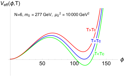
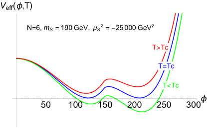
Figure 1: The effective potential at different temperature values for type-I PT (left) and type-II PT (right). Here, we considered the values $Q_{S}=0$ and $\lambda_{S}=0$.

IV Gravitational Waves from Phase Transitions

We analyze the gravitational waves (GWs) spectrum from first order EWPT in the model. In order to analyze the spectra, we introduce parameters, $\alpha$ and $\beta$, which characterize the GWs from the dynamics of vacuum bubble Grojean:2006bp . The parameter $\beta$ which describes approximately the inverse of time duration of the PT is defined as

$$\beta=-\left.\frac{dS_{E}}{dt}\right|_{t=t_{t}}\simeq\left.\frac{1}{\Gamma}\frac{d\Gamma}{dt}\right|_{t=t_{t}}.$$ (14)

where $S_{E}$ and $\Gamma$ are the Euclidean action of a critical bubble and vacuum bubble nucleation rate per unit volume and unit time at the time of the PT $t_{t}$, respectively. We use normalized parameter $\beta$ by Hubble parameter $H_{T}$ in the following analysis:

$$\tilde{\beta}=\frac{\beta}{H_{T}}=T_{t}\frac{d}{dT}\left(\frac{S_{3}(T)}{T}\right)\Bigg{|}_{T=T_{t}},$$ (15)

where $T_{t}$ is the transition temperature that is introduced by $\Gamma/H_{T}^{4}|_{T=T_{t}}=1$. The parameter $\alpha$ is the ratio of the released energy density

$$\epsilon(T)=-V_{eff}(\phi_{t}(T),T)+T\frac{\partial V_{eff}(\phi_{t}(T),T)}{\partial T},$$ (16)

where $\phi_{t}(T)$ is the true minimum at the temperature $T$, to the radiation energy density $\rho_{rad}=(\pi^{2}/30)g_{\ast}T^{4}$, where $g_{\ast}$ is relativistic degrees of freedom in the thermal plasma, at the transition temperature $T_{t}$:

$$\alpha=\frac{\epsilon(T_{t})}{\rho_{{\rm rad}}(T_{t})}.$$ (17)

The GWs production during a strong first order PT occurs via three co-existing mechanisms: (1) collisions of bubble walls and shocks in the plasma, where the so-called ” envelope approximation”  Kosowsky:1992rz can be used to describe this phenomenon and estimate the contribution of the scalar field to the GWs spectrum. (2) After the bubbles have collided and before expansion has dissipated the kinetic energy in the plasma, the sound waves could result significant contribution to the GWs spectrum Huber:2008hg . (3) Magnetohydrodynamic (MHD) turbulence in the plasma that is formed after the bubbles collision may also have give rise to the GWs spectrum Caprini:2006jb . Therefore, the stochastic GWs background could be approximated as

$$\Omega_{{\rm GW}}h^{2}=\Omega_{{\rm\phi}}h^{2}+\Omega_{{\rm sw}}h^{2}+\Omega_{{\rm tur}}h^{2}.$$ (18)

The importance of each contribution depends on the PT dynamics, and especially on the bubble wall velocity. Here, we focus on the contribution to GWs from the compression waves in the plasma (sound waves) which is the strongest GWs spectrum among the source of the total GW. A fitting function to the numerical simulations is obtained as Caprini:2015zlo

$$\Omega_{{\rm sw}}(f)h^{2}=\widetilde{\Omega}_{{\rm sw}}h^{2}\times(f/\tilde{f}_{{\rm sw}})^{3}\left(\frac{7}{4+3(f/\tilde{f}_{{\rm sw}})^{2}}\right)^{7/2},$$ (19)

where the peak energy density is

$$\widetilde{\Omega}_{{\rm sw}}h^{2}\simeq 2.65\times 10^{-6}v_{b}\tilde{\beta}^{-1}\left(\frac{\kappa\alpha}{1+\alpha}\right)^{2}\left(\frac{100}{g_{\ast}^{t}}\right)^{1/3},$$ (20)

at the peak frequency

$$\tilde{f}_{{\rm sw}}\simeq 1.9\times 10^{-5}\mbox{Hz}\frac{1}{v_{b}}\tilde{\beta}\left(\frac{T_{t}}{100{\rm GeV}}\right)\left(\frac{g_{\ast}^{t}}{100}\right)^{1/6},$$ (21)

where $v_{b}$ is the velocity of the bubble wall and $\kappa$ is the fraction of vacuum energy that is converted into bulk motion of the fluid. Contrary to what it was believed, a succesful electroweak baryogenesis and a sizable gravitational wave signal can be achived in the same setup Caprini:2007xq , where the GWs signal is in the reach of BBO and LISA for very fine-tuned scenario No:2011fi . Here, since we are interested in probing any possible GWs signal in a general SM extension that can map many models, we adopt the value $v_{b}=0.95$. Indeed, in a concreate model, one has to deal with many issues like CP violation source(s), the exact bubble wall and plasma velocities.

V Numerical Results

In our numerical results, we have three free parameters $\{N,m_{S},\omega\}$ where we consider the multiplicity values $N=2,6,12,24$, the scalar-Higgs doublet coupling range $\left|\omega\right|\leq 5$, and the scalar mass to lie in the range $m_{S}\in[100\,GeV,\,550\,GeV]$. In Fig. 2, we present the predicted values of $\alpha$ and $\tilde{\beta}$ for different values of $\{N,m_{S},\omega=2(m_{S}^{2}-\mu_{S}^{2})/\upsilon^{2}\}$ with $Q_{S}=1$ and $\lambda_{S}=0$.

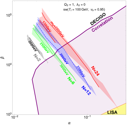
Figure 2: The predicted values of $\alpha$ and $\tilde{\beta}$ for different values of $\{N,m_{S},\omega\}$ with $Q_{S}=1$, $\lambda_{S}=0$ and $\mu_{S}^{2}\geq 0$.

In Fig. 2, the gray, red, blue and green regions represent $\{N=2,~{}6,~{}12,~{}24\}$, respectively. We also show the expected sensitivities of LISA and DECIGO detector configurations are set by using the sound wave contribution for $T_{t}=100~{}GeV$ and the bubble wall velocity $v_{b}$ = 0.95. The colored regions are experimental sensitivities reached at future space-based interferometers, LISA Klein:2015hvg ; Caprini:2015zlo ; PetiteauDataSheet and DECIGO Kawamura:2011zz .

In Fig. 3, we present the special case $\mu_{S}^{2}=0$. Both left and right panels represent the same results, where in the left panel we present information about parameter values and constraints, and in the right one we show the value of the EWPT strength parameter $\phi_{c}/T_{c}$.

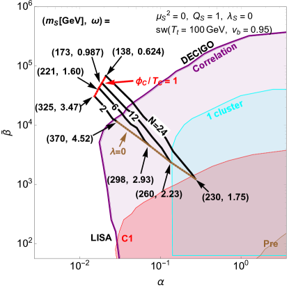
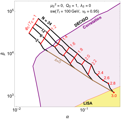
Figure 3: The predicted values of $\alpha$ and $\tilde{\beta}$ for different values of $\{N,m_{S},\omega\}$ with $Q_{S}=1$, $\lambda_{S}=0$ and $\mu_{S}^{2}=0$.

In Fig. 3, the black curves correspond to the special case $\mu_{S}^{2}=0$, for $\{N=2,~{}6,~{}12,~{}24\}$, and the upper bound (in red) on $\tilde{\beta}$ is set by the condition $\phi_{c}/T_{c}=1$. However, the lower bound (in brown) on $\tilde{\beta}$ is dictated by the vacuum stability condition (6). The label ”C1” in Fig. 3-left, corresponds to the configuration of LISA provided in Table. 1 in Caprini:2015zlo , whereas the labels ”Pre-DECIGO”, ”FP-DECIGO” and ”Correlation” are DECIGO designs Kawamura:2011zz . From this figure, one notices that for stronger PT with $\phi_{c}/T_{c}\geq 1.38$ the generated GWs can be seen by DECIGO, and for $\phi_{c}/T_{c}\geq 2.95$ the corresponding GWs can be seen by LISA.

In Fig. 4, we show the regions in the plane $\{m_{S},\omega\}$ where there exist a type-I and type-II PT for different multiplicity values $N$, together with the constraints mentioned in section II, such as the unitarity bound, the vacuum stability condition of $\lambda\geq 0$, and $R_{\gamma\gamma}^{\phi}$. In addition, we show few contours that express the relative enhancement in the triple Higgs coupling (8). In Fig. 4, the green (yellow) regions corresponds to the allowed regions by the experiemental measurments of the di-photon Higgs decay for $|Q_{S}|=1$ at the accuracy of $1\sigma$ ($2\sigma$). The thin ribbon in top-left of the cases $N=6,12,24$ is also part of the allowed region by the di-photon Higgs decay, which corresponds to the case where the $A_{0}(m_{S}^{2}/4m_{0}^{2})$ term in (7) has a value around -2.

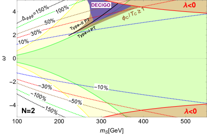
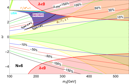
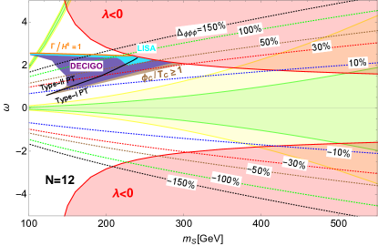
Figure 4: The area of the occurrence of detectable gravitational wave spectrum, the vacuum stability condition of $\lambda\geq 0$ and the constraint on $R_{\gamma\gamma}^{\phi}$. The dotted lines are the deviation of the triple coupling (8), and the red regions describe the vacuum stability condition (6). The green and yellow regions represent the current experimental data of $\phi\rightarrow\gamma\gamma$ at the accuracy of $1\sigma$ and $2\sigma$, respectively ATLAS:2018doi . The brown region represents the area of a strong PT without possible GWs detectabily, and the black line shows the border of Type-I and Type-II PT.

From Fig. 4, the GWs detectable region is different from one multiplicity value to another. If the new singlet is electrically charged $Q_{S}\neq 0$, the EWPT can not be strongly first order while fulfilling the constraint from $\phi\rightarrow\gamma\gamma$ ATLAS:2018doi for large multiplicity values $N>2$. In other models that contain scalars with opposite couplings to the Higgs doublet this conflict can be evaded, while the EWPT is still strongly first order. According to the multiplicity $N$, the scalar mass should lie between 120 GeV and 380 GeV in order to have a strong first order EWPT, i.e., type-I PT, and detectable GWs signal at DECIGO and may be LISA. However, detectable GWs signal can be observed even for $m_{S}<100~{}GeV$ for type-II PT, i.e., the EWPT is a second order transition (or a cross over); and the baryon asymsetry should be achieved via another mechanism rather than the EWB scenario.

In addition, one has to mention that detectable GWs signal implies positive enhancement on the triple Higgs coupling (8) with ratio between 10% to more than 150%, depending on the multiplicity $N$. The main idea one can learn from the results in Fig. 4 is that if the EWPT is strongly first order (type-I PT), the GWs signal would be able to be detected by the future space based GW interferometers, in addition to a non-negligible enhancement in triple Higgs coupling (8). If the EWPT is crossover or second order, there could exist another transition at a temperature value smaller that the EWPT where the system vacuum moves to a new, deeper and larger minimum via bubbles nucleation where it leaves also detectable signal (type-II PT) the future space based GW interferometers.

VI Conclusion

We have focused on the model with additional $N$ isospin singlet scalar fields $S$ which have hypercharge $Q_{S}$. In this model, we distinguish two types of EWPT: (1) type-I: the EW symmetry gets broken in one step where the system moves from the wrong vacuum ($\langle\phi\rangle=0$) to the true one ($\langle\phi\rangle\neq 0$); and (2) type-II: the EWPT occurs in two steps where the first one is a second order PT (or a crossover), and a new minimum ($\langle\phi_{2}\rangle\neq 0$) rather than the existing one ($\langle\phi_{2}\rangle>\langle\phi_{1}\rangle$) occurs which gets deeper as the temperature gets lower until it becomes the absolute minimum. Then, in the second step, the transition from $\langle\phi_{1}\rangle$ to $\langle\phi_{2}\rangle$ occurs via bubbles nucleation due to the existing barrier between the two minima.

We noticed also that GWs are large enough to be detected by future space-based interferometers, such as LISA and DECIGO, for the condition of strongly phase transition, in either type-I for a successful scenario of electroweak baryogenesis or type-II where baryogenesis can be fulfilled via another mechanism, there appear significant deviations in the Higgs couplings $\phi\phi\phi$ and $\phi\gamma\gamma$ from the SM predictions. We have discussed how the model can be tested by the synergy between collider experiments and GW observation experiments. Consequently, by the detection of the GWs and the measurement of $\phi\gamma\gamma$, we can test the model. Current experimental data for $\phi\gamma\gamma$ and the parameter region where detectable GW occur from the type-I PT can give a constraint on the number of additional singlet scalar $N\leq 6$.

Acknowledgments: K. H. was supported by the Sasakawa Scientific Research Grant from The Japan Science Society. S. K. was supported in part by Grant-in-Aid for Scientific Research on Innovative Areas, the Ministry of Education, Culture, Sports, Science and Technology, No. 16H06492 and No. 18H04587, Grant H2020-MSCA-RISE-2014 No. 645722 (Non-Minimal Higgs).

References

- (1) C. Patrignani et al. [Particle Data Group], Chin. Phys. C 40, no. 10, 100001 (2016).
- (2) A. D. Sakharov, Pisma Zh. Eksp. Teor. Fiz. 5, 32 (1967) [JETP Lett. 5, 24 (1967)] [Sov. Phys. Usp. 34, 392 (1991)] [Usp. Fiz. Nauk 161, 61 (1991)].
- (3) V. A. Kuzmin, V. A. Rubakov and M. E. Shaposhnikov, Phys. Lett. 155B, 36 (1985). M. E. Shaposhnikov, JETP Lett. 44, 465 (1986) [Pisma Zh. Eksp. Teor. Fiz. 44, 364 (1986)]. M. E. Shaposhnikov, Nucl. Phys. B 287, 757 (1987).
- (4) A. I. Bochkarev and M. E. Shaposhnikov, Mod. Phys. Lett. A 2, 417 (1987). K. Kajantie, M. Laine, K. Rummukainen and M. E. Shaposhnikov, Nucl. Phys. B 466, 189 (1996) [hep-lat/9510020].
- (5) G. W. Anderson and L. J. Hall, Phys. Rev. D 45, 2685 (1992). J. R. Espinosa and M. Quiros, Phys. Rev. D 76, 076004 (2007) [hep-ph/0701145]. J. R. Espinosa and M. Quiros, Phys. Lett. B 305, 98 (1993) [hep-ph/9301285]. A. Ahriche, Phys. Rev. D 75, 083522 (2007) [hep-ph/0701192]. S. Profumo, M. J. Ramsey-Musolf and G. Shaughnessy, JHEP 0708, 010 (2007) [arXiv:0705.2425 [hep-ph]]. A. Ahriche and S. Nasri, JCAP 1307, 035 (2013) [arXiv:1304.2055]. A. Ahriche and S. Nasri, Phys. Rev. D 85, 093007 (2012) [arXiv:1201.4614 [hep-ph]]. T.A. Chowdhury, M. Nemevsek, G. Senjanovic, and Y. Zhang, JCAP 1202, 029 (2012) [arXiv:1110.5334 [hep-ph]]. D. Borah and J.M. Cline, Phys. Rev. D 86, 055001 (2012) [arXiv:1204.4722 [hep-ph]]. G. Gil, P. Chankowski and M. Krawczyk, Phys. Lett. B 717, 396 (2012) [arXiv:1207.0084 [hep-ph]]. J. R. Espinosa, T. Konstandin and F. Riva, Nucl. Phys. B 854, 592 (2012) [arXiv:1107.5441 [hep-ph]]. A. Ahriche, K. L. McDonald and S. Nasri, Phys. Rev. D 92, no. 9, 095020 (2015) [arXiv:1508.05881 [hep-ph]]. M. Saeedhosini and A. Tofighi, Adv. High Energy Phys. 2017, 7638204 (2017) [arXiv:1701.02074 [hep-ph]].
- (6) X. m. Zhang, Phys. Rev. D 47, 3065 (1993) [hep-ph/9301277]. C. Grojean, G. Servant and J. D. Wells, Phys. Rev. D 71, 036001 (2005) [hep-ph/0407019]. C. Delaunay, C. Grojean and J. D. Wells, JHEP 0804, 029 (2008) [arXiv:0711.2511 [hep-ph]]. F. P. Huang, Y. Wan, D. G. Wang, Y. F. Cai and X. Zhang, Phys. Rev. D 94, no. 4, 041702 (2016) [arXiv:1601.01640 [hep-ph]]. R. G. Cai, M. Sasaki and S. J. Wang, JCAP 1708, no. 08, 004 (2017) [arXiv:1707.03001 [astro-ph.CO]].
- (7) J. M. Cline and P. A. Lemieux, Phys. Rev. D 55, 3873 (1997) [hep-ph/9609240]. G. C. Dorsch, S. J. Huber and J. M. No, JHEP 1310, 029 (2013) [arXiv:1305.6610 [hep-ph]]. P. Basler, M. Krause, M. Muhlleitner, J. Wittbrodt and A. Wlotzka, JHEP 1702, 121 (2017) [arXiv:1612.04086 [hep-ph]]. P. Basler, M. M ” uhlleitner and J. Wittbrodt, JHEP 1803, 061 (2018) [arXiv:1711.04097 [hep-ph]].
- (8) R. Apreda, M. Maggiore, A. Nicolis and A. Riotto, Nucl. Phys. B 631, 342 (2002) [gr-qc/0107033]. S. J. Huber and T. Konstandin, JCAP 0805, 017 (2008) [arXiv:0709.2091 [hep-ph]]. S. J. Huber, T. Konstandin, G. Nardini and I. Rues, JCAP 1603, no. 03, 036 (2016) [arXiv:1512.06357 [hep-ph]]. A. Ahriche and S. Nasri, Phys. Rev. D 83, 045032 (2011) [arXiv:1008.3106 [hep-ph]].
- (9) P. Huang, A. J. Long and L. T. Wang, Phys. Rev. D 94, no. 7, 075008 (2016) [arXiv:1608.06619 [hep-ph]]. P. Schwaller, Phys. Rev. Lett. 115, no. 18, 181101 (2015) [arXiv:1504.07263 [hep-ph]]. W. Chao, H. K. Guo and J. Shu, JCAP 1709, no. 09, 009 (2017) [arXiv:1702.02698 [hep-ph]]. Y. Chen, M. Huang and Q. S. Yan, arXiv:1712.03470 [hep-ph]. Y. Wan, B. Imtiaz and Y. F. Cai, arXiv:1804.05835 [hep-ph]. M. Aoki, S. Kanemura and O. Seto, Phys. Rev. Lett. 102, 051805 (2009), [arXiv:0807.0361 [hep-ph]]. M. Aoki, S. Kanemura and O. Seto, Phys. Rev. D 80, 033007 (2009), M. Aoki, S. Kanemura and K. Yagyu, Phys. Rev. D 83, 075016 (2011), [arXiv:1102.3412 [hep-ph]]. S. Kanemura, E. Senaha and T. Shindou, Phys. Lett. B 706, 40 (2011), [arXiv:1109.5226 [hep-ph]]. C. Tamarit, Phys. Rev. D 90, no. 5, 055024 (2014), [arXiv:1404.7673 [hep-ph]]. S. Kanemura, N. Machida and T. Shindou, Phys. Lett. B 738, 178 (2014), [arXiv:1405.5834 [hep-ph]]. K. Hashino, S. Kanemura and Y. Orikasa, Phys. Lett. B 752, 217 (2016), [arXiv:1508.03245 [hep-ph]].
- (10) S. Kanemura, Y. Okada and E. Senaha, Phys. Lett. B 606, 361 (2005) [hep-ph/0411354]. A. Noble and M. Perelstein, Phys. Rev. D 78, 063518 (2008) [arXiv:0711.3018 [hep-ph]].
- (11) B. P. Abbott et al. [LIGO Scientific and Virgo Collaborations], Phys. Rev. Lett. 116, no. 6, 061102 (2016) [arXiv:1602.03837 [gr-qc]]. B. P. Abbott et al. [LIGO Scientific and Virgo Collaborations], Phys. Rev. Lett. 116, no. 24, 241103 (2016) [arXiv:1606.04855 [gr-qc]].
- (12) M. Kamionkowski, A. Kosowsky and M. S. Turner, Phys. Rev. D 49, 2837 (1994) [astro-ph/9310044]. E. Witten, Phys. Rev. D 30, 272 (1984). C. J. Hogan, Mon. Not. Roy. Astron. Soc. 218, 629 (1986).
- (13) P. A. Seoane et al. [eLISA Collaboration], arXiv:1305.5720 [astro-ph.CO]. N. Bartolo et al., JCAP 1612, no. 12, 026 (2016) [arXiv:1610.06481 [astro-ph.CO]].
- (14) S. Kawamura et al., Class. Quant. Grav. 28, 094011 (2011).
- (15) V. Corbin and N. J. Cornish, Class. Quant. Grav. 23, 2435 (2006) [gr-qc/0512039].
- (16) X. Gong et al., J. Phys. Conf. Ser. 610, no. 1, 012011 (2015) [arXiv:1410.7296 [gr-qc]].
- (17) J. Luo et al. [TianQin Collaboration], Class. Quant. Grav. 33, no. 3, 035010 (2016) [arXiv:1512.02076 [astro-ph.IM]]. X. C. Hu et al., Class. Quant. Grav. 35, no. 9, 095008 (2018) [arXiv:1803.03368 [gr-qc]].
- (18) J. Kehayias and S. Profumo, JCAP 1003, 003 (2010). [arXiv:0911.0687 [hep-ph]]. A. D. Dolgov, D. Grasso and A. Nicolis, Phys. Rev. D 66, 103505 (2002). [astro-ph/0206461]. J. R. Espinosa, T. Konstandin, J. M. No and M. Quiros, Phys. Rev. D 78, 123528 (2008). [arXiv:0809.3215 [hep-ph]]. M. Kakizaki, S. Kanemura and T. Matsui, Phys. Rev. D 92, no. 11, 115007 (2015). [arXiv:1509.08394 [hep-ph]]. P. S. B. Dev and A. Mazumdar, Phys. Rev. D 93, no. 10, 104001 (2016). [arXiv:1602.04203 [hep-ph]]. K. Hashino, M. Kakizaki, S. Kanemura and T. Matsui, Phys. Rev. D 94, no. 1, 015005 (2016). [arXiv:1604.02069 [hep-ph]]. V. Vaskonen, Phys. Rev. D 95, no. 12, 123515 (2017) [arXiv:1611.02073 [hep-ph]]. M. Chala, G. Nardini and I. Sobolev, Phys. Rev. D 94, no. 5, 055006 (2016). [arXiv:1605.08663 [hep-ph]]. A. Kobakhidze, A. Manning and J. Yue, Int. J. Mod. Phys. D 26, no. 10, 1750114 (2017). [arXiv:1607.00883 [hep-ph]]. A. Addazi, Mod. Phys. Lett. A 32, no. 08, 1750049 (2017). [arXiv:1607.08057 [hep-ph]]. K. Hashino, M. Kakizaki, S. Kanemura, P. Ko and T. Matsui, Phys. Lett. B 766, 49 (2017) [arXiv:1609.00297 [hep-ph]]. Z. Kang, P. Ko and T. Matsui, JHEP 1802, 115 (2018) [arXiv:1706.09721 [hep-ph]]. W. Chao, W. F. Cui, H. K. Guo and J. Shu, [arXiv:1707.09759 [hep-ph]]. L. Marzola, A. Racioppi and V. Vaskonen, Eur. Phys. J. C 77, no. 7, 484 (2017) [arXiv:1704.01034 [hep-ph]]. S. V. Demidov, D. S. Gorbunov and D. V. Kirpichnikov, Phys. Lett. B 779, 191 (2018) [arXiv:1712.00087 [hep-ph]]. M. Chala, C. Krause and G. Nardini, JHEP 1807, 062 (2018) [arXiv:1802.02168 [hep-ph]]. K. Hashino, M. Kakizaki, S. Kanemura, P. Ko and T. Matsui, JHEP 1806, 088 (2018) [arXiv:1802.02947 [hep-ph]]. T. Vieu, A. P. Morais and R. Pasechnik, arXiv:1802.10109 [hep-ph]. S. Bruggisser, B. Von Harling, O. Matsedonskyi and G. Servant, arXiv:1803.08546 [hep-ph]. F. P. Huang, Z. Qian and M. Zhang, Phys. Rev. D 98, no. 1, 015014 (2018) [arXiv:1804.06813 [hep-ph]]. S. Bruggisser, B. Von Harling, O. Matsedonskyi and G. Servant, arXiv:1804.07314 [hep-ph]. M. F. Axen, S. Banagiri, A. Matas, C. Caprini and V. Mandic, arXiv:1806.02500 [astro-ph.IM]. A. Alves, T. Ghosh, H. K. Guo and K. Sinha, arXiv:1808.08974 [hep-ph]. E. Megias, G. Nardini and M. Quiros, arXiv:1806.04877 [hep-ph]. J. Ellis, M. Lewicki and J. M. No, arXiv:1809.08242 [hep-ph].
- (19) K. Hashino, R. Jinno, M. Kakizaki, S. Kanemura, T. Takahashi and M. Takimoto, arXiv:1809.04994 [hep-ph].
- (20) S.P. Martin, Phys. Rev. D65,116003 (2002) [hep-ph/0111209].
- (21) C. S. Chen, C. Q. Geng, D. Huang and L. H. Tsai, Phys. Rev. D 87, 075019 (2013) [arXiv:1301.4694 [hep-ph]].
- (22) The ATLAS collaboration [ATLAS Collaboration], ATLAS-CONF-2018-031.
- (23) A. Ahriche, A. Arhrib and S. Nasri, JHEP 1402, 042 (2014) [arXiv:1309.5615 [hep-ph]].
- (24) S. Kanemura, S. Kiyoura, Y. Okada, E. Senaha and C. P. Yuan, Phys. Lett. B 558, 157 (2003) [hep-ph/0211308]. S. Kanemura, Y. Okada, E. Senaha and C.-P. Yuan, Phys. Rev. D 70, 115002 (2004) [hep-ph/0408364].
- (25) [CMS Collaboration], arXiv:1307.7135 [hep-ex].
- (26) J. Brau et al. [ILC Collaboration], arXiv:0712.1950 [physics.acc-ph]. A. Djouadi et al. [ILC Collaboration], arXiv:0709.1893 [hep-ph]. N. Phinney et al., arXiv:0712.2361 [physics.acc-ph]. T. Behnke et al. [ILC Collaboration], arXiv:0712.2356 [physics.ins-det]. ibitemBehnke:2013lya T. Behnke et al., arXiv:1306.6329 [physics.ins-det]. H. Baer, et al. ” Physics at the International Linear Collider ” , Physics Chapter of the ILC Detailed Baseline Design Report: http://lcsim.org/papers/DBDPhysics.pdf
- (27) E. Accomando et al. [CLIC Physics Working Group], hep-ph/0412251; L. Linssen, A. Miyamoto, M. Stanitzki and H. Weerts, arXiv:1202.5940 [physics.ins-det].
- (28) M. Bicer et al. [TLEP Design Study Working Group], JHEP 1401, 164 (2014) [arXiv:1308.6176 [hep-ex]].
- (29) ATLAS Collaboration, ATL-PHYS-PUB-2014-019 (2014); ATLAS Collaboration, ATL-PHYS-PUB-2015-046 (2015).
- (30) D. M. Asner et al., arXiv:1310.0763 [hep-ph]; G. Moortgat-Pick et al., Eur. Phys. J. C 75, no. 8, 371 (2015) [arXiv:1504.01726 [hep-ph]]; K. Fujii et al., arXiv:1506.05992 [hep-ex].
- (31) C. Guella, D. Cherigui, A. Ahriche, S. Nasri and R. Soualah, Phys. Rev. D 93, no. 9, 095022 (2016) [arXiv:1601.04342 [hep-ph]].
- (32) A. Ahriche, S. Nasri and R. Soualah, Phys. Rev. D 89, no. 9, 095010 (2014) [arXiv:1403.5694 [hep-ph]].
- (33) D. Cherigui, C. Guella, A. Ahriche and S. Nasri, Phys. Lett. B 762, 225 (2016) [arXiv:1605.03640 [hep-ph]].
- (34) Q. H. Cao, G. Li, K. P. Xie and J. Zhang, Phys. Rev. D 97, no. 11, 115036 (2018) [arXiv:1711.02113 [hep-ph]].
- (35) Q. H. Cao, G. Li, K. P. Xie and J. Zhang, arXiv:1810.07659 [hep-ph].
- (36) L. Dolan and R. Jackiw, Phys. Rev. D9, 3320 (1974). Weinberg, Phys. Rev. D9,3357 (1974).
- (37) M. E. Carrington, Phys. Rev. D45, 2933 (1992).
- (38) D. J. Gross, R. D. Pisarski and L. G. Yaffe, Rev. Mod. Phys. 53, 43 (1981). R. R. Parwani, Phys. Rev. D 45, 4695 (1992) Erratum: [Phys. Rev. D 48, 5965 (1993)] [hep-ph/9204216]. P. B. Arnold and O. Espinosa, Phys. Rev. D 47, 3546 (1993) Erratum: [Phys. Rev. D 50, 6662 (1994)] [hep-ph/9212235].
- (39) A. Ahriche and S. Nasri, JCAP1307 (2013) 035 [arXiv:1304.2055[hep-ph]]. A. Ahriche,G. Faisel,S. Y. Ho, S. Nasri and J. Tandean, Phys. Rev. D92 (2015) no.3, 035020 [arXiv:1501.06605[hep-ph]]. A. Ahriche, K. L. McDonald and S. Nasri, Phys. Rev. D92 (2015) no.9, 095020 [arXiv:1508.05881[hep-ph]]. A. Ahriche, S. M. Boucenna and S. Nasri, Phys. Rev. D93 (2016) no.7, 075036 [arXiv:1601.04336[hep-ph]].
- (40) C. Grojean and G. Servant, Phys. Rev. D 75, 043507 (2007).
- (41) A. Kosowsky, M. S. Turner and R. Watkins, Phys. Rev. Lett. 69, 2026 (1992). A. Kosowsky, M. S. Turner and R. Watkins, Phys. Rev. D 45, 4514 (1992). A. Kosowsky and M. S. Turner, Phys. Rev. D 47, 4372 (1993) [astro-ph/9211004]. M. Kamionkowski, A. Kosowsky and M. S. Turner, Phys. Rev. D 49, 2837 (1994) [astro-ph/9310044].
- (42) S. J. Huber and T. Konstandin, JCAP 0809, 022 (2008) [arXiv:0806.1828 [hep-ph]]. M. Hindmarsh, S. J. Huber, K. Rummukainen and D. J. Weir, Phys. Rev. Lett. 112, 041301 (2014) [arXiv:1304.2433 [hep-ph]]. J. T. Giblin, Jr. and J. B. Mertens, JHEP 1312, 042 (2013) [arXiv:1310.2948 [hep-th]]. J. T. Giblin and J. B. Mertens, Phys. Rev. D 90, no. 2, 023532 (2014) [arXiv:1405.4005 [astro-ph.CO]]. M. Hindmarsh, S. J. Huber, K. Rummukainen and D. J. Weir, Phys. Rev. D 92, no. 12, 123009 (2015) [arXiv:1504.03291 [astro-ph.CO]].
- (43) C. Caprini and R. Durrer, Phys. Rev. D 74, 063521 (2006) [astro-ph/0603476]. T. Kahniashvili, A. Kosowsky, G. Gogoberidze and Y. Maravin, Phys. Rev. D 78, 043003 (2008) [arXiv:0806.0293 [astro-ph]]. T. Kahniashvili, L. Campanelli, G. Gogoberidze, Y. Maravin and B. Ratra, Phys. Rev. D 78, 123006 (2008) Erratum: [Phys. Rev. D 79, 109901 (2009)] [arXiv:0809.1899 [astro-ph]]. T. Kahniashvili, L. Kisslinger and T. Stevens, Phys. Rev. D 81, 023004 (2010) [arXiv:0905.0643 [astro-ph.CO]]. C. Caprini, R. Durrer and G. Servant, JCAP 0912, 024 (2009) [arXiv:0909.0622 [astro-ph.CO]]. L. Kisslinger and T. Kahniashvili, Phys. Rev. D 92, no. 4, 043006 (2015) [arXiv:1505.03680 [astro-ph.CO]].
- (44) C. Caprini et al., JCAP 1604, no. 04, 001 (2016) [arXiv:1512.06239 [astro-ph.CO]].
- (45) C. Caprini, R. Durrer and G. Servant, Phys. Rev. D 77, 124015 (2008) [arXiv:0711.2593 [astro-ph]].
- (46) J. M. No, Phys. Rev. D 84, 124025 (2011) [arXiv:1103.2159 [hep-ph]].
- (47) A. Klein et al., Phys. Rev. D 93, no. 2, 024003 (2016) [arXiv:1511.05581 [gr-qc]].
-
(48)
Data sheet by A. Petiteau,
http://www.apc.univ-paris7.fr/Downloads/lisa/eLISA/Sensitivity/Cfgv1/StochBkgd/