Magnetic and topological transitions in three-dimensional topological Kondo insulator

Abstract

By using an extended slave-boson method, we draw a global phase diagram summarizing both magnetic phases and paramagnetic (PM) topological insulating phases (TI_s) in three-dimensional topological Kondo insulator (TKI). By including electron hopping (EH) up to third neighbor, we identify four strong topological insulating (STI) phases and two weak topological insulating (WTI) phases, then the PM phase diagrams characterizing topological transitions between these TI_s are depicted as functions of EH, $f$-electron energy level and hybridization constant. We also find an insulator-metal transition from a STI phase which has surface Fermi rings and spin textures in qualitative agreement to TKI candidate SmB₆. In weak hybridization regime, antiferromagnetic (AF) order naturally arises in the phase diagrams, and depending on how the magnetic boundary crosses the PM topological transition lines, AF phases are classified into AF topological insulator (AFTI) and non-topological AF insulator (nAFI), according to their $\mathcal{Z}_{2}$ indices. In two small regions of parameter space, two distinct topological transition processes between AF phases occur, leading to two types of AFTI, showing distinguishable surface dispersions around their Dirac points.

Over the recent years, searching topological phases of matter has becoming one of the central topics in condensed matter physics. Zhang11 Among the enlarging family of topological matters, the strongly correlated electron systems offer as important basis, because they naturally involve rich kinds of mechanism, hence can generate a variety of interacting topological phases, such as interacting topological insulator, Go12 topological Mott insulator, Yu11 interacting topological superconductor, Wang12 Weyl semimetal, Wan11 topological Kondo insulator, Dzero12 antiferromagnetic topological insulator (AFTI), Mong10 ; Fang13 ; ZhiLi15 ; Li18 etc.

Topological Kondo insulator (TKI), Dzero12 a heavy-fermion system with strong Coulomb interaction and $d$-$f$ hybridization governing by spin-orbit coupling, preserves time-reversal symmetry (TRS), therefore can generate topological insulating phases (TI_s) with Kondo screening effect. As revealed by previous works, variation of electron hopping (EH) strength, $f$-electron energy level $\epsilon_{f}$ and hybridization constant $V$ can drive topological transitions among phases of strong topological insulator (STI), weak topological insulator (WTI) and normal Kondo insulator (nKI). Legner14 However, existing works in literature are restricted to their interested parameter regime, hence the studied TI_s are still confined to a limited number of STI and WTI, and the full STI and WTI phases in TKI have not been explored adequately, particularly at the presence of strong electron-electron correlation. Legner14 In this work, by considering adequate parameter space of periodic Anderson model (PAM), we uncover all possible TI_s in three-dimensional (3D) TKI: four STI and two WTI, each possessing distinct surface states and Dirac cones. We also present the paramagnetic (PM) phase diagrams characterizing topological transitions between these TI_s, as functions of EH, $\epsilon_{f}$ and $V$. By proper fitting of EH, we verify a STI phase with Fermi surfaces and spin textures which can qualitatively simulate the TKI material SmB₆, Xu16 confirming the applicability of PAM to TKI, and it is find that this STI phase is in vicinity to an insulator-metal transition driving by enhancement of $V$.

In heavy-fermion systems, the interplay and competition between Kondo screening and magnetic correlation can motivate magnetic transitions when the Kondo interaction is reduced. Vekic95 Similarly, in half-filled TKI, theoretical calculations have verified a transition to AF phase when the hybridization interaction $V$ is weakened, Li18 ; Peters18 reminiscent of the induced magnetism in pressurized SmB₆. Butch16 ; Zhao17 ; Chang17 Besides, our earlier work has proved that due to the combined $\mathcal{S}$ symmetry of time reversal and translation operations, the AF states in TKI remain topological distinguishable, regardless of the breaking of TRS by magnetic order. We has developed a $\mathcal{Z}_{2}$ topological classification to the AF states in TKI and proposed a novel AFTI phase under unique setting of model parameters, together with an AFTI-nontopological AF insulator (nAFI) topological transition while EH was shifted in some way. Li18 Unfortunately, why AFTI should appear in such parameter region is still not clear, and it remains confused whether new AF phases exist in other parameter regions. We have shown that at least near the magnetic boundary (MB), the $\mathcal{Z}_{2}$ index for AF directly relies on that of TI phase from which the AF order develops, Li18 therefore, in order to investigate all possible AF phases with distinct topologies, the magnetic transition and classification of AF phases should be discussed on the basis of the PM phase diagrams summarizing all TI_s, i.e., the four STI and two WTI should be included properly to study the AF transition as well as the topological transitions between AF phases.

We use the spin-1/2 PAM to character the 3D TKI in cubic lattice: Alexandrov15

$$H=H_{d}+H_{f}+H_{df}+H_{U},$$ (1)

where $H_{d}=\sum_{\mathbf{k},\alpha}(\epsilon^{d}_{\mathbf{k}}-\mu)d^{\dagger}_{\mathbf{k}\alpha}d_{\mathbf{k}\alpha}$, $H_{f}=\sum_{\mathbf{k},\alpha}(\epsilon_{f}+\epsilon^{f}_{\mathbf{k}}-\mu)f^{\dagger}_{\mathbf{k}\alpha}f_{\mathbf{k}\alpha}$. $H_{df}=V\sum_{\mathbf{k},\alpha,\beta}\mathbf{S}_{\mathbf{k}}\cdot\vec{\sigma}_{\alpha\beta}d^{\dagger}_{\mathbf{k}\alpha}f_{\mathbf{k}\beta}+h.c.$ is the Kondo hybridization with spin-orbit coupling, in which $\mathbf{S}_{\mathbf{k}}=(\sin\mathbf{k}\cdot\mathbf{a}_{1},\sin\mathbf{k}\cdot\mathbf{a}_{2},\sin\mathbf{k}\cdot\mathbf{a}_{3})$, Alexandrov15 with the element vectors $\mathbf{a}_{1}$, $\mathbf{a}_{2}$, $\mathbf{a}_{3}$ for cubic lattice. $H_{U}=U\sum_{i}n^{f}_{i\uparrow}n^{f}_{i\downarrow}$ is the on-site coulomb repulsion between $f$ electrons, and we consider infinite $U$ in this work. We includes EH up to third neighbor, with $t_{d(f)}$, $t^{\prime}_{d(f)}$, $t^{\prime\prime}_{d(f)}$ denote nearest-neighbor (NN), next-nearest-neighbor (NNN), and next-next-nearest-neighbor (NNNN) hopping amplitudes, respectively, which determine the tight-binding dispersions $\epsilon^{d(f)}_{\mathbf{k}}$. The chemical potential $\mu$ is used to fix the total electron number to half filling $n_{t}=2$, and variable EH, hybridization interaction $V$ and $f$ energy level $\epsilon_{f}$ are considered. In what follows, $t_{d}=1$ is set as energy unit, and we choose $t_{f}=-0.2$ and keep $t^{\prime}_{d}/t_{d}=t^{\prime}_{f}/t_{f}$ to get a medium gapped insulating phase (unless when the insulator-metal transition is discussed).

We employ the Kotliar-Ruckenstein (K-R) slave-boson method Kotliar86 ; Sun93 ; Li18 to solve PAM. Similar to Coleman’s slave boson theory, Alexandrov15 the mean-field approximation of PAM Eq. 1 in large-$U$ limit reads Li18

$$H_{MF}=N(-\eta n_{f})$$

$$+\sum_{\mathbf{k},\alpha,\beta}(d^{\dagger}_{\mathbf{k}\alpha},f^{\dagger}_{\mathbf{k}\alpha})\left(\begin{array}[]{cc}(\epsilon^{d}_{\mathbf{k}}-\mu)\delta_{\alpha\beta}&\tilde{V}\mathbf{S}_{\mathbf{k}}\cdot\vec{\sigma}_{\alpha\beta}\\ \tilde{V}\mathbf{S}_{\mathbf{k}}\cdot\vec{\sigma}_{\alpha\beta}&(\tilde{\epsilon}^{f}_{\mathbf{k}}-\mu)\delta_{\alpha\beta}\end{array}\right)\left(\begin{array}[]{cc}d^{\dagger}_{\mathbf{k}\beta}\\ f^{\dagger}_{\mathbf{k}\beta}\end{array}\right),$$ (6)

where the effective hybridization $\tilde{V}=VZ$ is renormalized by factor $Z=\sqrt{2(1-n_{f})/(2-n_{f})}$, and the effective $f$ dispersion $\tilde{\epsilon}^{f}_{\mathbf{k}}=\epsilon_{f}+\eta+Z^{2}\epsilon^{f}_{\mathbf{k}}$, in which $\eta$ shifts the $f$ level. $n_{f}$ is the density of $f$ electron per site, N is the number of lattice sites. The PM mean field parameters $n_{f}$, $\eta$, $\mu$ are solvable through saddle-point solution for $H_{MF}$, then the quasi-particle dispersions which are the eigenvalues of the Hamiltonian matrix in Eq. 6 (in a modified form) are used to identify the $\mathcal{Z}_{2}$ index.

Table 1: Parameters and $\mathcal{Z}_{2}$ invariants of the TI phases shown in Fig. 1. In all phases, $t_{f}=-0.2$.

phase	$t^{\prime}_{d}$	$t^{\prime\prime}_{d}$	$t^{\prime}_{f}$	$t^{\prime\prime}_{f}$	$\epsilon_{f}$	$V$	$\delta_{\Gamma}$	$\delta_{X}$	$\delta_{M}$	$\delta_{R}$	$\nu_{0}$	$\nu_{j}$	Dirac points
STI${}_{\bar{\Gamma}}$	0.26	0.26	-0.052	-0.052	-2	0.7	1	-1	-1	-1	1	-	$\bar{\Gamma}$
STI${}_{\bar{\Gamma}\bar{X}}$	-0.35	-0.35	0.07	0.07	-2	1	-1	1	-1	-1	1	-	$\bar{\Gamma}$, $\bar{X}$
STI${}_{\bar{M}}$	0.252	0.252	-0.0504	-0.0504	-2	1.5	1	1	1	-1	1	-	$\bar{M}$
STI${}_{\bar{M}\bar{X}}$	0.4	0	-0.08	0	-1	1	1	1	-1	1	1	-	$\bar{M}$, $\bar{X}$
WTI${}_{\bar{\Gamma}\bar{M}}$	-0.6	0	0.12	0	-1	1	-1	1	1	-1	0	1	$\bar{\Gamma}$, $\bar{M}$
WTI${}_{\bar{X}}$	-0.2	0	0.04	0	-2	1	1	1	-1	-1	0	1	$\bar{X}$

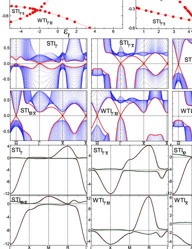
Figure 1: First row: PM phase diagrams of 3D TKI. Parameters: $t_{f}=-0.2$, $t^{\prime}_{f}/t_{f}=t^{\prime}_{d}/t_{d}$, (a) $V=1$, $t^{\prime\prime}_{d}=t^{\prime\prime}_{f}=0$; (b) $\epsilon_{f}=-2$, $t^{\prime\prime}_{d}=t^{\prime}_{d}$, $t^{\prime\prime}_{f}=t^{\prime}_{f}$. Second and third rows: slab dispersions of TI_s. The red lines denote the surface states. Last two rows: quasi-particle dispersions (black solid lines) in six TI_s, the red and green lines are $d$- and renormalized $f$- dispersions, respectively. Parameters and $\mathcal{Z}_{2}$ invariants for each TI_s are listed in Tab. 1.

In last two rows of Fig. 1, we show six types of distinct quasi-particle spectrums of PM TI_s, each with different model parameters listed in Tab. 1, comparing with $d$ and $f$ dispersions. At the eight high symmetric points (HSP_s) $\mathbf{k}_{m}$ in 3D Brillouin zone (BZ) (i.e.,$\Gamma$=(0,0,0); $X$=($\pi$,0,0), (0,$\pi$,0), (0,0,$\pi$); $M$=($\pi$,$\pi$,0), ($\pi$,0,$\pi$), (0,$\pi$,$\pi$); and $R$=($\pi$,$\pi$,$\pi$)), the hybridization vanishes (due to its odd parity), consequently the quasi-particle energy equals either $\epsilon^{d}_{\mathbf{k}}$ or $\tilde{\epsilon}^{f}_{\mathbf{k}}$, leading to the parity of occupied states $\delta_{m}=$ 1 or -1 at $\mathbf{k}_{m}$, respectively. Therefore, the strong topological index $\nu_{0}$ can be easily obtained by observing the bulk dispersions in Fig. 1 via $(-1)^{\nu_{0}}=\prod_{m\in\mathrm{HSP}_{s}}\delta_{m}$, and the weak topological indices $\nu_{j}$ ($j=x,y,z$) are calculated from the HSP_s on $k_{j}$ plane $P_{j}$ through $(-1)^{\nu_{j}}=\prod_{m\in P_{j}}\delta_{m}$. Dzero12 The quantities $\delta_{m}$ and $\mathcal{Z}_{2}$ indices for six TI_s are listed in Tab. 1.

By diagonalizing 40 slabs to simulate the 3D lattice with opened (001) surface, the surface states of the six TI_s are computed and displayed by second and third rows in Fig. 1. On (001) surface, there are four HSP_s: $\bar{\Gamma}$=(0,0); $\bar{X}$=($\pi$,0), (0,$\pi$); and $\bar{M}$=($\pi$,$\pi$), each of the six TI_s in Fig. 1 has Dirac points locating at different HSP_s. The requirement of odd number of Dirac points on surface of STI leads to four inequivalent STI_s: STI${}_{\bar{\Gamma}}$, STI${}_{\bar{M}}$, STI${}_{\bar{\Gamma}\bar{X}}$, and STI${}_{\bar{M}\bar{X}}$, in which the subscripts denote the locations of Dirac points. For WTI_s, there are even number of Dirac points, resulting in two WTI_s: WTI${}_{\bar{\Gamma}\bar{M}}$ and WTI${}_{\bar{X}}$. For nKI, generally no Dirac point exists, however, there is a special nKI with Dirac points at all four HSP_s, since Fermi level crosses its surface states even times between two arbitrary HSP_s, this phase is actually non-topological phase rather than a topological one.

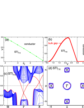
Figure 2: (a) Insulator-metal transition from STI${}_{\bar{\Gamma}\bar{X}}$ to conducting phase. (b) Closing of bulk gap during this transition. (c) Slab dispersions of STI${}_{\bar{\Gamma}\bar{X}}$. (d) Surface Fermi rings and spin textures of STI${}_{\bar{\Gamma}\bar{X}}$. $t^{\prime}_{d}=t^{\prime\prime}_{d}=-0.375$, $t_{f}=-0.23$, $t^{\prime}_{f}=t^{\prime\prime}_{f}=0.2$. $\epsilon_{f}=-4$ for (b) to (d), and $V=1$ for (c) and (d).

In the first row of Fig. 1, with varying $t^{\prime}_{d}$, $\epsilon_{f}$ and $V$, we have located the topological boundaries among all possible TI_s, determining by the change of $\mathcal{Z}_{2}$ index. The topological transitions between TI_s are generated by closing and reopening of the insulating gap at certain HSP, leading to an inversion of parity and consequently the shifting of $\mathcal{Z}_{2}$ index. Li18

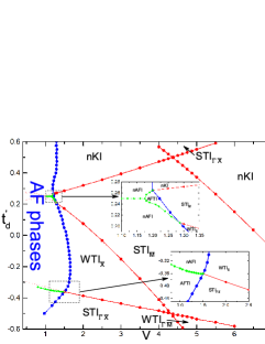
Figure 3: (a) Magnetic boundary in 3D TKI (blue lines). Near $t^{\prime}_{d}=0.25$ and $-0.35$, topological transitions between AF phases take place (green solid lines). Parameters: $\epsilon_{f}=-1.5$, $t^{\prime\prime}_{d}=t^{\prime}_{d}$, $t^{\prime\prime}_{f}=t^{\prime}_{f}$, $t_{f}=-0.2$ and $t^{\prime}_{f}/t_{f}=t^{\prime}_{d}/t_{d}$.

In above, we have set $t^{\prime}_{f}/t_{f}=t^{\prime}_{d}/t_{d}$, under which the Dirac points in TI_s all cross the Fermi energy, leading to the vanishment of Fermi surface. For TKI candidate SmB₆, medium-sized surface Fermi rings around $\bar{\Gamma}$ and $\bar{X}$ were detected through ARPES, verifying it in a STI${}_{\bar{\Gamma}\bar{X}}$ phase. Xu16 Though our study of TKI is based on the simplified PAM, it can still produce a STI${}_{\bar{\Gamma}\bar{X}}$ with similar surface states to SmB₆. To do this, we chose EH departing from $t^{\prime}_{f}/t_{f}=t^{\prime}_{d}/t_{d}$, and found a STI${}_{\bar{\Gamma}\bar{X}}$ phase with Fermi surfaces and helical spin textures quite similar to SmB₆, see Fig. 2(c) and (d). Furthermore, this phase is in vicinity to an insulator-metal transition generated by shifting of $V$ or $\epsilon_{f}$ (see Fig. 2(a) and (b)), which may be account for the metallic phase observed in pressurized SmB₆. Paraskevas15 ; Zhao17

Based on the PM phase diagrams of TI_s, we now study the AF transitions in TKI. In our previous work, the original K-R method of symmetric PAM Kotliar86 ; Sun93 has been generalized to treat AF phases in non-symmetric case, Li18 which can be applied to TKI. The resulting mean-field Hamiltonian is rather complicated in that in addition to $n_{f}$, $\eta$ and $\mu$, two AF order parameters $m_{f}$ and $h$ should be determined, besides, two renormalization factors $Z_{1}$ and $Z_{2}$ arise. Due to the $\mathcal{S}$ symmetry combined by TRS and lattice translation, the AF phases in TKI fall into $\mathcal{Z}_{2}$ topological class, and the $\mathcal{Z}_{2}$ index $\nu$ is calculated from the parities of the occupied spectrums at four Kramers degenerate momenta (KDM) $\mathbf{p}_{m}$ ($\Gamma$ and three $X$ points) via $(-1)^{\nu}=\prod_{\mathbf{p}_{m}\in\mathrm{KDM}}\delta_{m}$, in which $\delta_{m}=\prod_{i}\xi_{i}(\mathbf{p}_{m})$, with the parity $\xi_{i}(\mathbf{p}_{m})$ of $i$-th occupied state at $\mathbf{p}_{m}$ equals either 1 or -1, when quasi-particle energy equals that of $d$ or $f$ at $\mathbf{p}_{m}$, respectively. Li18 Particularly, the strong topological index $\nu_{0}$ on the PM side of the MB directly determines $\nu$ of the AF phase near MB, namely, $\nu_{0}=1$ (STI) leads to $\nu=1$ (AFTI), while $\nu_{0}=0$ (WTI or nKI) leads to $\nu=0$ (nAFI), Mong10 ; Li18 giving a straightforward verification of the AF phases near MB.

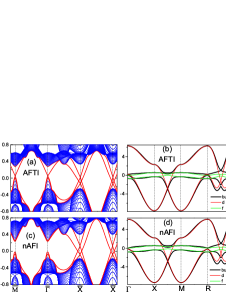
Figure 4: Surface dispersions (left column) and quasi-particle dispersions (right column) of AFTI and nAFI near the AF topological boundary in lower inset of Fig. 3. $V=1.4$, $t^{\prime}_{d}=-0.37$ for AFTI, and $t^{\prime}_{d}=-0.35$ for nAFI.

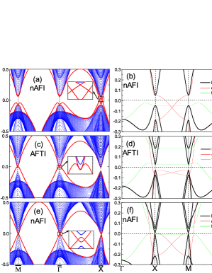
Figure 5: Surface spectrums (left column) and quasi-particle dispersions (right column) of the three AF phases near the AF topological boundary in upper inset of Fig. 3. $V=1.19$ for all. From up, middle to down rows, $t^{\prime}_{d}=0.235$, $0.253$, and $0.264$, respectively.

The magnetic critical hybridization $V_{c}$ is calculated as a function of $t^{\prime}_{d}$, then the MB plotted by $V_{c}$ is added to the phase diagram, see Fig. 3. The MB crosses the topological boundaries of TI_s in two parts, one near $t^{\prime}_{d}=0.25$, the other around $t^{\prime}_{d}=-0.35$, see insets of Fig. 3 for details.

Around $t^{\prime}_{d}=-0.35$, the MB is divided by the STI${}_{\bar{\Gamma}\bar{X}}$-WTI${}_{\bar{X}}$ transition line into two parts, leading to AFTI and nAFI just below the two parts of MB, respectively. While $V$ is lowered further from MB, $\nu$ of AF phases should be computed from the 3D spectrums (e.g., Fig. 4 (b) and (d)) to determine the AFTI-nAFI topological boundary, which is demonstrated by the green line near $t^{\prime}_{d}=-0.35$ in Fig. 3. The AFTI-nAFI transition is realized via parity inversion during gap closing and reopening at $\Gamma$, and it converges with STI${}_{\bar{\Gamma}\bar{X}}$-WTI${}_{\bar{X}}$ boundary at the MB, see the lower inset in Fig. 3.

Near $t^{\prime}_{d}=0.25$, the MB is separated by WTI${}_{\bar{X}}$-STI${}_{\bar{M}}$ and STI${}_{\bar{M}}$-nKI lines into three parts. Below the middle part of MB (which touches STI${}_{\bar{M}}$), an AFTI arises, while below the other two parts of MB, nAFI emerges. The AFTI-nAFI transition forms a narrow water-drop-shaped area in which AFTI survives (green solid line in the upper inset in Fig. 3). Besides, though nAFI_s above and below $t^{\prime}_{d}=0.25$ have quite different dispersions (compare Fig. 5(b) with (f)), they still have equal $\nu=0$, since their magnetic orders grow from nKI and WTI, respectively. Though band gap is closed at the boundary between two nAFI_s, no parity inversion occurs, consequently no topological transition takes place (see the green dashed line in upper inset of Fig. 3).

The surface states of AF phases are shown in Fig. 4(a), (c) near $t^{\prime}_{d}=-0.35$, and in Fig. 5(a), (c), (e) around $t^{\prime}_{d}=0.25$, respectively. In AFTI_s, the Dirac points at $\bar{\Gamma}$ and $\bar{M}$ are protected by topology hence are robust, see Fig. 4(a) and Fig. 5(c). Furthermore, the Dirac surface states of two AFTI_s (one near STI${}_{\bar{M}}$ and the other near STI${}_{\bar{\Gamma}\bar{X}}$) disperse quite differently, in which the former constructs a valley shape (Fig. 5(c)). In contrast, the gapless surface states at $\bar{X}$ in both AFTI and nAFI (Fig. 4(a), (c) and Fig. 5(a)) are not robust, since they can be gapped by additional factor such as gate voltage. Li18

In summary, we have performed a slave-boson mean-field analysis of the 3D TKI using spin-orbit coupled PAM, and presented the phase diagrams including all possible PM TI_s in TKI: four STI and two WTI, each with distinguishable locations of Dirac points. We also obtained a STI${}_{\bar{\Gamma}\bar{X}}$ phase with similar surface states to SmB₆, and found it can be driven to conducting state through an insulator-metal transition by enhanced hybridization. We also investigated the magnetic boundary of AF phases in TKI, and found the topological transitions between AFTI and nAFI in two narrow regions in parameter space. Besides, we found two types of AFTI with distinct dispersions at the Dirac points. Though our work is based on an uniform mean-field approximation, any site-dependent treatment will not break the application of $\mathcal{Z}_{2}$ classification of both PM and AF states. Peters18 ; Chang17 We hope our work can help to reach a comprehensive understanding of novel AFTI phases in strongly correlated electrons systems.

References

- (1) Qi X L and Zhang S C 2011 Rev. Mod. Phys. 83, 1057
- (2) Go A et al 2012 Phys. Rev. Lett. 109, 066401
- (3) Yu S L, Xie X C and Li J X 2011 Phys. Rev. Lett. 107,010401
- (4) Wang Z and Zhang S C 2012 Phys. Rev. B 86, 165116
- (5) Wan X G et al 2011 Phys. Rev. B 83, 205101
- (6) Dzero M el al 2012 Phys. Rev. B 85, 045130
- (7) Mong R S K, Essin A M and Moore J E 2010 Phys. Rev. B 81, 245209
- (8) Fang C, Gilbert M J and Bernevig B A 2013 Phys. Rev. B 88, 085406
- (9) Li Z et al 2015 Phys. Rev. B 91, 235128
- (10) Li H et al 2018 J. Phys.: Condens. Matter https://doi.org/10.1088/1361-648X/aae17b
- (11) Legner M, Rüegg A and Sigrist M 2014 Phys. Rev. B 89, 085110
- (12) Xu N, Ding H and Shi M 2016 J. Phys.: Condens. Matter 28, 363001
- (13) Vekic M et al 1995 Phys. Rev. Lett. 74, 2367
- (14) Peters R, Yoshida T and Kawakami N 2018 Phys. Rev. B 98, 075104
- (15) Zhou Y Z el al 2017 Science Bulletin 62, 1439
- (16) Butch N P el al 2016 Phys. Rev. Lett. 116, 156401
- (17) Chang K W and Chen P J 2018 Phys. Rev. B 97, 195145
- (18) Alexandrov V, Coleman P, and Erten O 2015 Phys. Rev. Lett. 114, 177202
- (19) Kotliar G and Ruckenstein A E 1986 Phys. Rev. Lett. 57, 1362
- (20) Sun S J, Yang M F and Hongt T M 1993 Phys. Rev. B 48, 16127
- (21) Paraskevas P, Martin B and Mohamed M 2015 Europhys. Letts. 110, 66002