Cluster formation in the W40 and Serpens South complex triggered by the expanding H ii region

Abstract

We present results of the mapping observations covering a large area of 1 square degree around W40 and Serpens South carried out in the ¹²CO ($J=1-0$), ¹³CO ($J=1-0$), C¹⁸O ($J=1-0$), CCS ($J_{N}$=8${}_{7}-7_{6}$), and N₂H⁺ ($J=1-0$) emission lines with the 45 m Nobeyama Radio Telescope. W40 is a blistered H ii region, and Serpens South is an infrared dark cloud accompanied by a young cluster. The relationship between these two regions which are separated by $\sim 20\arcmin$ on the sky has not been clear so far. We found that the C¹⁸O emission is distributed smoothly throughout the W40 and Serpens South regions, and it seems that the two regions are physically connected. We divided the C¹⁸O emission into four groups in terms of the spatial distributions around the H ii region which we call 5, 6, 7, and 8 km s^-1 components according to their typical LSR velocities, and propose a three-dimensional model of the W40 and Serpens South complex. We found two elliptical structures in position-velocity diagrams, which can be explained as a part of two expanding shells. One of the shells is the small inner shell just around the H ii region, and the other is the large outer shell corresponding to the boundary of the H ii region. Dense gas associated with the young cluster of Serpens South is likely to be located at the surface of the outer shell, indicating that the natal clump of the young cluster is interacting with the outer shell being compressed by the expansion of the shell. We suggest that the expansion of the shell induced the formation of the young cluster.

1 Introduction

OB stars give significant influence on the physical and chemical environments of the natal clumps, and trigger formation of the new generation of stars (e.g., Elmegreen & Lada, 1977). Investigation of star formation around the H ii regions is therefore essential to understand how star formation occurs and evolves by the influence of H ii regions.

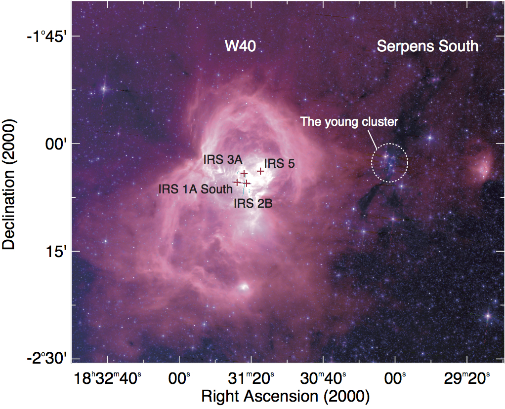
Figure 1: The W40 and Serpens South regions shown in a three-color composite image made with the $8.0\micron$ (red), $5.8\micron$ (green) and $4.5\micron$ (blue) data by $\it{Spitzer}$. The plus signs indicate the positions of the high mass infrared sources IRS 1A South, IRS 2B, IRS 3A, and IRS 5 (Smith et al., 1985; Shuping et al., 2012).

W40 and Serpens South, a part of the Aquila cloud complex, are deeply embedded in dust and gas. Several infrared (IR) observations have revealed the global dust distributions of the two regions. In figure 1, we show an overview of the two regions in a three-color composite image of the 8.0  (red), 5.8  (green) and 4.5  (blue) emission from the $\it{Spitzer}$ $\it{Space}$ $\it{Telescope}$ (hereafter, $\it{Spitzer}$). Recent VLBA parallax measurements by Ortiz-León et al. (2017) indicate a distance of $436\pm 9$ pc for both W40 and Serpens South.

W40 is a blister-type H ii region (e.g., Vallee, 1987) excited by a massive OB star cluster and is characterized by the ‘hourglass-shaped structure’ (Rodney & Reipurth, 2008) which was revealed by infrared observations using the $\it{Midcourse}$ $\it{Space}$ $\it{Experiment}$ and $\it{Spitzer}$. The hourglass-shaped structure consists of two interconnected cavities having an extent of $17\arcmin\times 30\arcmin$ oriented with one lobe to the southeast and the other to the northwest (Rodney & Reipurth, 2008). Shuping et al. (2012) conclude that the O9.5 star named IRS 1A South is the dominant source of Lyman continuum luminosity needed to power the H ii region, and is the likely source of the stellar wind that has made the hourglass-shaped structure. The dynamical age of the H ii region has been estimated to be $0.19-0.78$ Myr (Mallick et al., 2013). There are dense molecular clumps in and around the H ii region (e.g., Dobashi et al., 2005; Dobashi, 2011; Shimoikura et al., 2015; Rumble et al., 2016; Shimajiri et al., 2017). In our previous study with the ¹²CO ($J=3-2$) and HCO⁺ ($J=4-3$) emission lines (Shimoikura et al., 2015), we presented an evidence that the velocity field of the region shows a great complexity consisting of at least four distinct velocity components, and two of the components at 5 km s^-1 and 10 km s^-1 are likely to be tracing dense gas interacting with the expanding shell around the H ii region. Hundreds of young stellar objects (YSOs) are associated with the region, indicating active on-going star formation (e.g., Kuhn et al., 2010; Bontemps et al., 2010; Maury et al., 2011; Mallick et al., 2013). Kuhn et al. (2010) suggested that the YSOs are young with an age of $\leq 1$ Myr. These results suggest that the YSOs may be the second generation stars born by the influence of the expanding shell of W40. However, the previous studies were limited to a small area just around the H ii region, not covering the entire W40 region. It is therefore not yet evident how far the interstellar medium around W40 is affected by the ionization front.

Toward the $\sim 20^{\prime}$ west to the W40 region, there is another star-forming region Serpens South. This region can be recognized as a filamentary obscuring structure in the $\it{Spitzer}$ image (see figure 1). A young cluster has been found around the center of the structure (Gutermuth et al., 2008). The cluster consists of a large fraction of protostars, some of which blow out the powerful collimated outflows (Nakamura et al., 2011), indicating that they formed within 0.5 Myr in the past (Gutermuth et al., 2008). The filamentary structure was found to consist of multiple smaller filaments identified by gas and dust observations (e.g., Kirk et al., 2013; Nakamura et al., 2014; Fernández-López et al., 2014; Könyves et al., 2015). These filaments show velocity gradients along their elongation (e.g., Kirk et al., 2013; Nakamura et al., 2014; Fernández-López et al., 2014). Kirk et al. (2013) suggested that the velocity gradient in one of the filaments is due to gas accretion toward the central young cluster. On the other hand, Fernández-López et al. (2014) pointed out that the velocity gradients along the filaments can be interpreted as a projection of large-scale turbulence, as they also found an existence of velocity gradients perpendicular to the main axes of the filaments. On a larger scale, results of low resolution molecular observations ($\sim 3\arcmin$) covering both W40 and Serpens South by Nakamura et al. (2017) infer that the two regions might be physically connected. In that case, we wonder how much the Serpens South region can be influenced by the W40 H ii region. Though each region has been widely studied individually, their relationship has remained unclear to date.

The IR observations as shown in figure 1 can reveal only a part of the relationship of W40 and Serpens South, and they provide information neither on the internal structure nor the velocity field. To better illustrate the larger-scale view of the surroundings of W40 and Serpens South and to better understand the relationship between the two regions, large-scale mapping observations in molecular emission lines with a high angular resolution is needed.

In this work, we mapped the whole region shown in figure 1 in some molecular lines using the 45 m telescope at Nobeyama Radio Observatory (NRO). This study is based on ‘the Star Formation Legacy project’ which is a large-scale survey project of molecular gas in star-forming regions. The outline of the project will be described in a forthcoming paper (Nakamura et al. 2018, in preparation). Results of wide-field polarimetric observations toward Serpens South is given in Kusune et al. (2018, in preparation; see also Sugitani et al. 2011). Results of molecular line observations toward other star-forming regions will be presented in separate articles (Dobashi et al. 2018, in preparation: Nakamura et al. 2018, in preparation: Shimoikura et al. 2018b, in preparation: Tanabe et al. 2018, in preparation ).

The present study intends to understand the complex spatial and velocity structures of both the W40 and Serpens South regions by analyzing the molecular data. We adopt a distance of 436 pc to the observed area (Ortiz-León et al., 2017) in this paper.

We present the observational procedures in Section 2. In Section 3, we show the global distributions of the molecular gas. We also describe results of the analyses of the temperature distributions and velocity fields. In addition, we investigate the morphology and kinematics of the observed regions. Our conclusions are summarized in Section 4.

2 Observations

2.1 Observations with the NRO 45 m telescope

Molecular observations were performed by using the NRO 45 m telescope. The observations were carried out for $\sim 150$ hours in total in the period from 2015 April to 2017 March. The ¹²CO (115.271204 GHz), ¹³CO (110.201354 GHz), C¹⁸O (109.782176 GHz), CCS (93.870098GHz), and N₂H⁺ (93.1737637 GHz) emission lines were observed simultaneously using the on-the-fly (OTF) mode. The half-power beam width of the telescope at 110 GHz is $\sim 15\arcsec$, corresponding to $\sim 6500$ au at a distance of 436 pc. We mapped an area of $\sim 1$ square degree around W40 and Serpens South in these lines.

We used the multi-beam receiver “FOREST” (FOur beam REceiver System on the 45-m Telescope, Minamidani et al., 2016) as the frontend to obtain the large maps. The typical system temperatures were 170 K at 110 GHz. The backend used was the digital spectrometers SAM45 having a bandwidth of 31.25 MHz and a frequency resolution of 15.26 kHz. The frequency resolution corresponds to a velocity resolution of $\sim 0.04$ km s^-1 at 110 GHz. For intensity calibration, the chopper-wheel method (Kutner & Ulich, 1981) was used. The telescope pointing was checked by observing the SiO maser source V1111-Oph every 1.5 hour, which was found to be accurate within $\sim 5\arcsec$. We also observed a small region ($\sim 1\farcm 5\times 1\farcm 5$) in Serpens South every time we tuned the receiver to check the intensity calibration, and we found that the intensity fluctuations for all of the lines are less than $10\%$.

The spectra were reduced by fitting the baseline with linear functions, and the data were converted to 3-dimensional data with a spheroidal convolution at an angular grid of $7\farcs 5$ and a velocity resolution of 0.1 km s^-1. The velocity resolution was smoothed to this value to achieve a high signal to noise ratio. We used the NOSTAR software package (Sawada et al., 2008) for the reduction. We finally obtained the spectral data with an effective angular resolution of $\sim 22\arcsec$ at 110 GHz.

Following the calibration formulae available at the NRO website, we estimated the main beam efficiencies of the 45 m telescope for the ¹²CO, ¹³CO, C¹⁸O, CCS, and N₂H⁺ lines to be 0.416, 0.435, 0.437, 0.497, and 0.500, respectively, and used them to convert the obtained $T_{\rm a}^{*}$ scale data to $T_{\rm mb}$ scale data. One sigma noise level of the reduced data is $\Delta T_{\rm mb}=0.8-0.3$ K for the $\sim 0.1$ km s^-1 velocity resolution. The observed molecular lines and the resulting noise levels are summarized in table 1.

2.2 Archival data

We used $\it{Herschel}$ archive data from $\it{Herschel}$ Gould Belt survey (HGBS), i.e., the 70, 250, 500 $\micron$ maps, dust temperature map, and column density map of the observed region (André et al., 2010; Könyves et al., 2015). We also used $\it{Spitzer}$ data obtained from the public $\it{Spitzer}$ archive. These infrared data are used to compare with the molecular lines data.

3 Results and Discussion

3.1 The molecular distributions

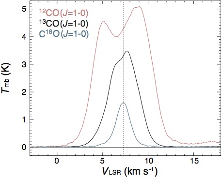
Figure 2: The ¹²CO, ¹³CO, and ${\rm C^{18}O}$ spectra averaged over the pixels detected at the $>5\sigma$ noise level. The vertical dashed line indicates the peak radial velocity of the averaged ${\rm C^{18}O}$ spectrum ($V_{\rm LSR}=7.3$ km s^-1).

In figure 2, we show the ¹²CO, ¹³CO, and C¹⁸O spectra averaged over the observed region. The C¹⁸O spectrum has a single peak at $V_{\rm LSR}=7.3$ km s^-1. There is a dip in the ¹²CO and ¹³CO spectra at this velocity, which should be due to absorption by colder gas in the foreground.

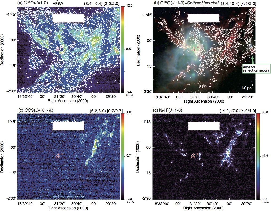
Figure 3: Velocity-integrated intensity maps of the (a) C¹⁸O, (c) CCS, and (d) N₂H⁺ emission lines, respectively. Velocity ranges in units of km s^-1 used for the integration are shown in the parentheses, and the contour levels of the lowest / intervals in units of K km s^-1 are shown in the brackets above each panel. In panel (b), the ${\rm C^{18}O}$ map (white contours) is overlaid on a composite color image of $Herschel$ 500  (red), 70  (green), and $Spitzer$ 8.0  (blue).

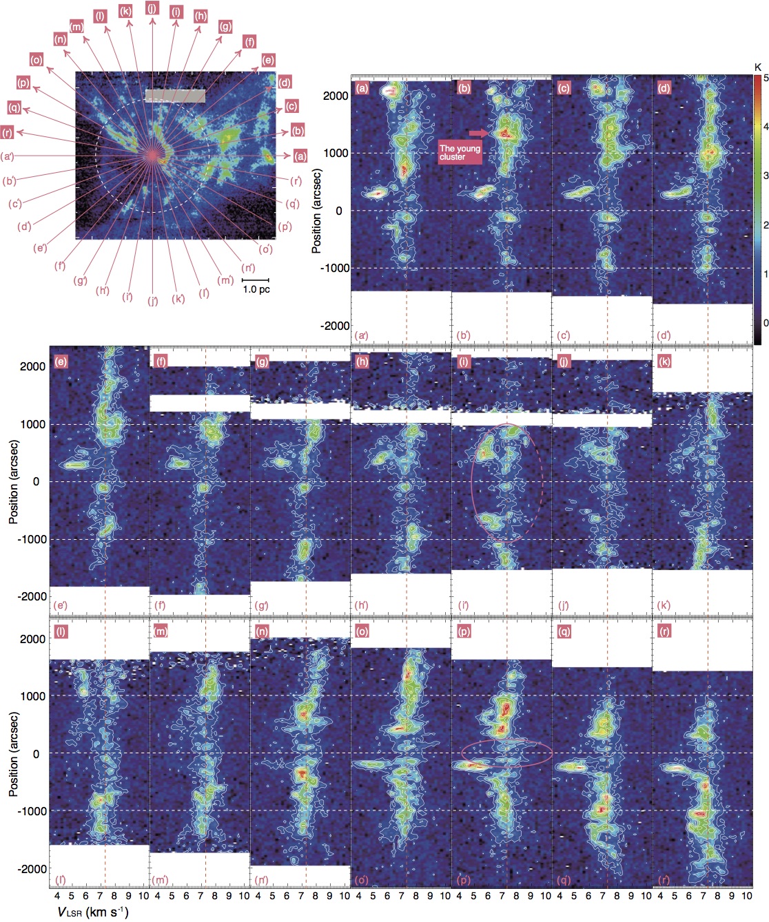
Figure 14: Position-velocity diagrams of the C¹⁸O emission line taken along the cuts (a)–(r) shown in the C¹⁸O intensity map at the top-left panel. The lowest contour and the contour interval are both 0.6 K. The horizontal-vertical red broken line indicates the systemic velocity ($V_{\rm LSR}=7.3$ km s^-1). The white broken lines indicate the position of IRS1A South as well as the positions separated by $\pm 1000\arcsec$ from the source roughly corresponding to the boundary of the H ii region. Two elliptical structures are marked with a pink ellipse in panels i and p.

Figure 3 shows the integrated intensity maps of the C¹⁸O, N₂H⁺, and CCS emission lines for the W40 and Serpens South regions. As seen in figure 3a, the C¹⁸O distributions around the densest parts of the W40 and Serpens South regions are similar to the structures found in our previous studies (e.g., Shimoikura et al., 2015; Nakamura et al., 2014). The figure clearly shows that the C¹⁸O emission is distributed over the entire observed area continuously. In addition, as we will show later, radial velocities of the emission line change smoothly over the observed area (e.g., see figure 14). We therefore conclude that the W40 and Serpens South regions are physically connected.

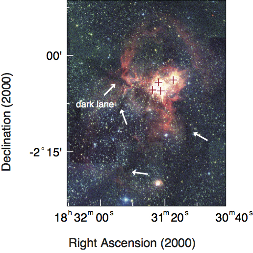
Figure 4: Composite image of W40 made with $\it{Spitzer}$ $8\micron$ (red), 2MASS $K$s (green), and $H$ (blue). Some dark lanes are shown with a white arrow.

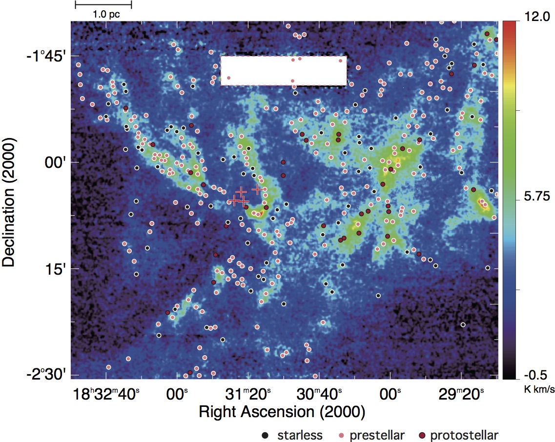
Figure 5: Distributions of cores reported by André et al. (2010) and Könyves et al. (2015) shown on the ${\rm C^{18}O}$ map. Starless, prestellar, and protostellar cores are indicated by black, pink, and red circles, respectively. The starless cores are the cores without YSO candidates and the prestellar cores are the cores with YSO candidates (see, Könyves et al., 2015).

In figure 3b, we also show the C¹⁸O intensity map overlaid on the composite image of $\it{Herschel}$ $500$ $\micron$ (red), $70$ $\micron$ (green), and $\it{Spitzer}$ $8$ $\micron$ (blue). The C¹⁸O emission is well correlated spatially with the dust emission revealed by $\it{Herschel}$ showing several dust filaments. We also show a composite image around W40 made from $\it{Spitzer}$ $8$ $\micron$, 2MASS $K$s, and $H$ bands in figure 4. We can see some dark lanes absorbed by dust, which can be seen in the dust emission in the $\it{Herschel}$ image. These dust filaments seem to be connected with Serpens South across the H ii region, and are associated with the C¹⁸O emission. One of the filaments is located at the waist of the hourglass structure, and it is known that many YSOs are associated with this dark lane (e.g., Kuhn et al., 2010; Maury et al., 2011; Mallick et al., 2013) as seen in figure 5 which shows the distributions of young cores around W40 and Serpens South cataloged by André et al. (2010) and Könyves et al. (2015).

In figure 3b, we also found that the H ii region is sharply outlined by a cavity of the C¹⁸O emission: There is less C¹⁸O emission in the southeast side of the W40 region as well as in the region between W40 and Serpens South, and such regions coincide well with the extent of the H ii region seen as the bright blue region in the $\it{Spitzer}$ image.

In figures 3c and 3d, elongated filamentary structures are detected with the CCS and N₂H⁺ emission lines. The CCS and N₂H⁺ emission lines are dominant toward a part corresponding to the main body of Serpens South. The morphology of the N₂H⁺ emission around the main body well matches with that of the dust emission detected by $Herschel$ (shown in red in figure 3b), which is consistent with the previous studies (Kirk et al., 2013; Nakamura et al., 2014). We also found that the region showing the N₂H⁺ emission around the OB cluster is compact, suggesting that the N₂H⁺ emission is enhanced around the OB cluster due to the high temperatures. The CCS emission is not detected in the W40 region above the $3\sigma$ noise level, as we already found in our previous study with CCS ($J_{N}=4_{3}-3_{2}$) (Shimoikura et al., 2015). In Serpens South, we found that the CCS intensity peak does not coincide with the N₂H⁺ peak corresponding to the position of the young cluster. The CCS emission is the strongest at $\sim 8\arcmin$ north to the N₂H⁺ intensity peak, and from there, it extends to the northwest in the map (figure 3c). Observations of HC₇N by Friesen et al. (2013) also show that the strong molecular emission extends to the north of the young cluster, showing similar distributions seen in our CCS map.

In earlier studies, the CCS and N₂H⁺ emission lines were surveyed only in a limited region around the OB cluster in W40 (e.g., Pirogov et al., 2013; Shimoikura et al., 2015) or around the main body of the Serpens South (e.g., Kirk et al., 2013; Nakamura et al., 2014). Our maps reveal the overall distributions of these molecular lines in W40 and Serpens South, and we found that they are detected at some positions along the dust filaments as well as in dust condensations in the H ii region, not only in the main body of the Serpens South.

From the above results, we found that the ionization front clearly delineates the boundary between the ionized region and the molecular gas. The morphology of the C¹⁸O distribution shows that W40 and Serpens South are molecular clouds in the same system, and that they are shaped by the expansion of the H ii region.

In addition, we found an extended C¹⁸O emitting region which may be a reflection nebula in the west of Serpens South. The distribution is consistent with one of the $\it{Herschel}$ dust filaments, and only a part of it is detected in N₂H⁺ and CCS on the north side of the filament.

3.2 The temperature distributions

In figure 3, we found that there is an anti-correlation between the C¹⁸O emission and the $\it{Spitzer}$ image, and the molecular gas seems to be influenced by the H ii region. To investigate the influence of the H ii region, we first estimated the excitation temperature $T_{\rm ex}$ for each observed molecular line throughout the observed region. For the estimation, we assumed the Local Thermodynamic Equilibrium (LTE) and that the observed emission lines are optically thin.

Under the LTE condition, $T_{\rm mb}$ is expressed by the following radiative transfer equation,

$$T_{\rm mb}=[J(T_{\rm ex})-J(T_{\rm bg})][1-{\rm exp}(-\tau(v))]\$$ (1)

where $J(T)=T_{0}/(e^{T_{0}/T}-1)$, $T_{0}=h\nu/k$, and $T_{\rm bg}=2.73$ K. Here, $\nu$ is the rest frequency of the emission line, $k$ is the Boltzmann constant, $h$ is the Planck constant, and $\tau(v)$ is the optical depth as a function of velocity.

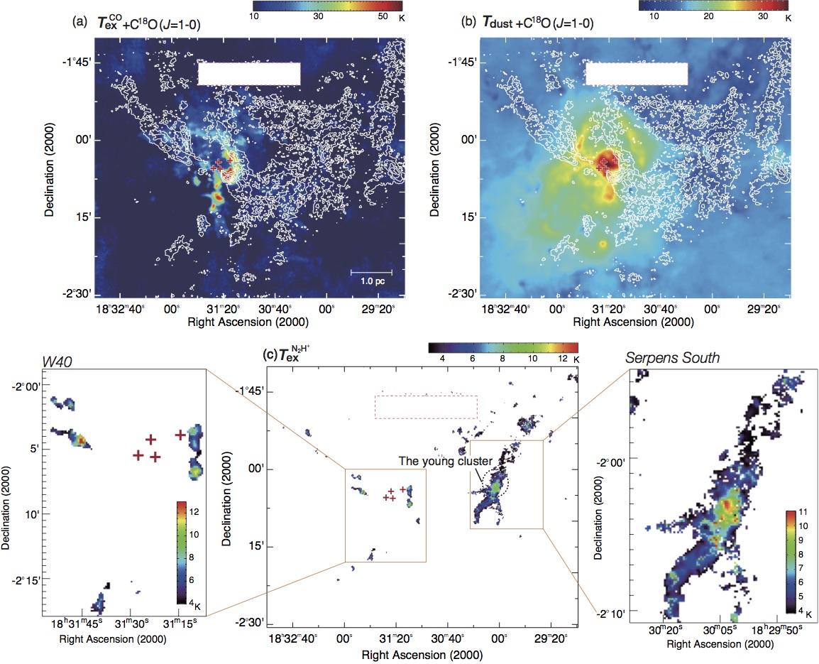
Figure 6: (a) Excitation temperature map derived from the ¹²CO ($J=1-0$) data. (b) Dust temperature map (André et al., 2010; Könyves et al., 2015). (c) Excitation temperature map of N₂H⁺ ($J=1-0$) (middle), and the close-up view of the W40 region (left) and the Serpens South region (right). The ${\rm C^{18}O}$ intensity map in figure 3a is overlaid in panels (a) and (b) by the white contours. The lowest contour and the contour interval are 4 K km s^-1 and 2 K km s^-1.

We estimated $T_{\rm ex}$ of C¹⁸O that we denoted as $T^{\rm{co}}_{\rm ex}$ from the $T_{\rm mb}$ data of the optically thick ¹²CO line ($\tau\gg 1$) by measuring the maximum value in the ¹²CO spectra. Line parameters of the molecules were taken from Splatalogue. The $T^{\rm{co}}_{\rm ex}$ map obtained by using equation (1) is shown in figure 6a. In figure 6b, we also show the dust temperature map $T_{\rm dust}$ for comparison, which is obtained by the $\it{Herschel}$ observations (André et al., 2010; Könyves et al., 2015).

For the N₂H⁺ molecule, we estimated the line parameters including the excitation temperature $T^{\rm{N{{}_{2}}H^{+}}}_{\rm ex}$ as follows: The N₂H⁺ ($J=1-0$) line has seven hyperfine components (e.g., Caselli et al., 1995). Because all of the components have the same $T^{\rm{N{{}_{2}}H^{+}}}_{\rm ex}$ and line width ${\Delta V}$, we performed a simultaneous fit with seven Gaussian components to the observed N₂H⁺ ($J=1-0$) spectrum at each position using equation (1). Here, $\tau(v)$ for the N₂H⁺ line can be expressed as

$${\tau}(v)={\tau_{\rm tot}}\sum_{i=1}^{7}C_{i}{\rm exp}\frac{{-(v-V_{0}+v_{i})^{2}}}{{2\,\sigma_{i}}^{2}}$$ (2)

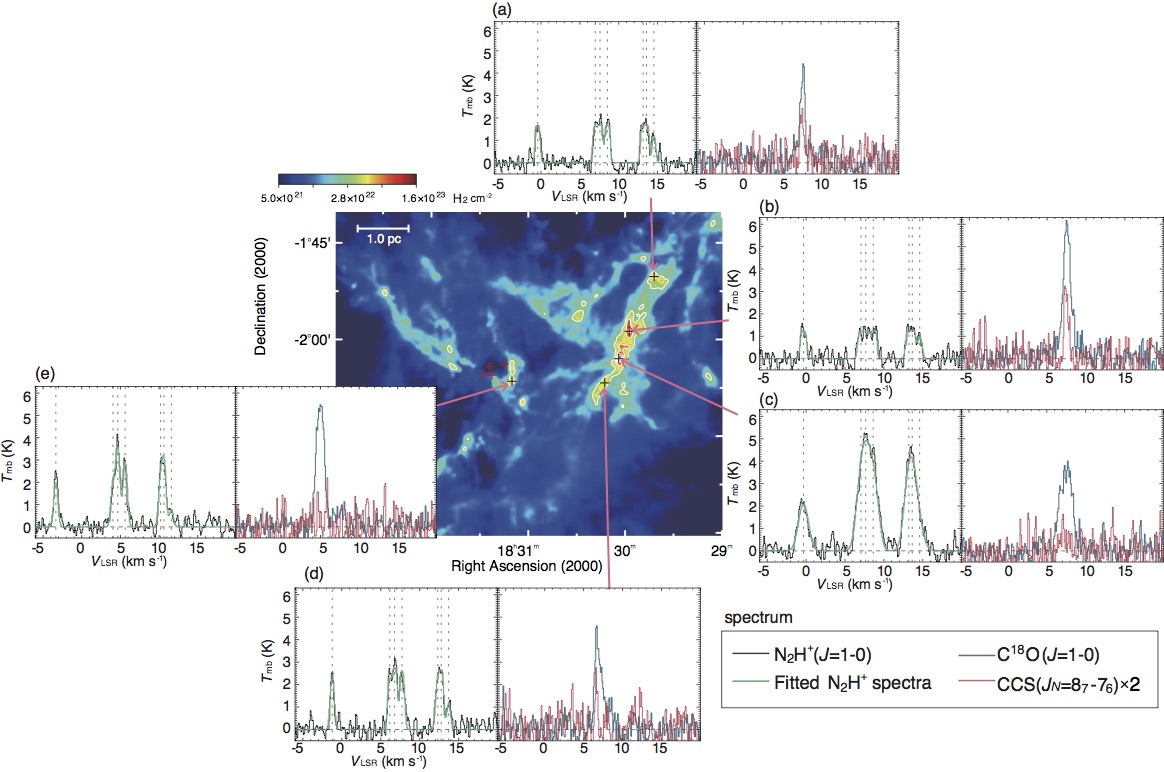
Figure 7: ${\rm C^{18}O}$ , N₂H⁺ , and CCS spectra observed at some positions indicated by the black plus signs. Results of the hyperfine fit of the N₂H⁺ spectra are also shown. The map in the middle represents the $N$(H₂) distribution derived from the $\it{Herschel}$ data in units of cm^-2 (e.g., André et al., 2010). The lowest contour and the contour interval of the $N$(H₂) map are $3\times 10^{22}$ cm^-2.

where $C_{i}$ is the normalized relative intensity (i.e., $\sum_{i=1}^{7}C_{i}=1$) and $v_{i}$ is the artificial velocity difference due to the slight differences of the rest frequencies. The parameters for the estimations are taken from Tiné et al. (2000) and Splatalogue. $\sigma_{i}$ is the velocity dispersion that can be expressed as ${\Delta V}/\sqrt{8{\rm ln}2}$ where $\Delta V$ is the velocity dispersion measured at full width at half maximum (FWHM). We selected positions where the N₂H⁺ emission is detected with $\geq 10$ $\sigma$, and performed the fitting to derive the total optical depth of the seven hyperfine components $\tau_{\rm tot}$, the peak LSR velocity $V_{0}$, ${\Delta V}$, $T_{\rm mb}$, and $T^{\rm{N{{}_{2}}H^{+}}}_{\rm ex}$ of each position. We show the fitted values of $T^{\rm{N{{}_{2}}H^{+}}}_{\rm ex}$ across the observed region in figure 6c. In figure 7, we also show an example of the observed and fitted N₂H⁺ spectra together with the ${\rm C^{18}O}$ and CCS spectra measured at some positions. Here, the derived parameters of N₂H⁺ at the position shown in figure 7c are $V_{0}=7.66\pm 0.01$ km s^-1, $\tau_{\rm tot}=3.18\pm 0.06$, ${\Delta V}=1.72\pm 0.03$ km s^-1, and $T^{\rm{N{{}_{2}}H^{+}}}_{\rm ex}=10.16\pm 0.40$ K. Similarly, the parameters at the position shown in figure 7e are $V_{0}=4.65\pm 0.01$ km s^-1, $\tau_{\rm tot}=4.24\pm 0.11$, ${\Delta V}=0.70\pm 0.01$ km s^-1, and $T^{\rm{N{{}_{2}}H^{+}}}_{\rm ex}=8.47\pm 0.70$ K.

In figure 6a, the $T^{\rm{co}}_{\rm ex}$ reaches a value of $56$ K in the vicinity of the OB cluster, whereas $T^{\rm{co}}_{\rm ex}$ around the Serpens region stays around $\sim 10$ K and exceeds 15 K only around the young cluster. We note that the derived values of $T^{\rm{co}}_{\rm ex}$ are the lower limits since the ¹²CO line often shows heavy self-absorption around $\sim 7$ km s^-1 as seen in figure 2. The $T_{\rm dust}$ map clearly shows that the distribution is similar to the shape of the H ii region traced by $\it{Spitzer}$, showing decreasing temperature with increasing distance from the ionized gas. Here, N₂H⁺ will be destroyed by CO evaporated from grain surfaces at 25 K (e.g., Lee et al., 2004). We found that $T_{\rm dust}$ around the OB cluster is higher than 25 K. As shown in figure 3d, the N₂H⁺ emission around the OB cluster is compact, and we thus suggest that the N₂H⁺ molecule is largely destroyed by CO evaporated from dust. In the Serpens South region, there is a tendency that the temperature becomes higher around the young cluster in figure 6c: The $T^{\rm{N{{}_{2}}H^{+}}}_{\rm ex}$ is $>5$ K, which increases to $\sim 11$ K in the dense regions where the young cluster is located. The temperature around the young cluster is also high in the $T_{\rm dust}$ map.

The temperature distributions of $T^{\rm{co}}_{\rm ex}$, $T_{\rm dust}$, and $T^{\rm{N{{}_{2}}H^{+}}}_{\rm ex}$ roughly show a similar tendency: All of the maps show a trend of decreasing temperature with increasing distance from the H ii region, suggesting that the molecular gas and dust in W40 are warmed by the radiation from the OB cluster.

3.3 The velocity structure

To investigate the global velocity structures, we made mean velocity $V_{0}$ map of the ${\rm C^{18}O}$ , CCS, and N₂H⁺ emission lines. For ${\rm C^{18}O}$ and CCS, $T_{\rm mb}$ was measured through fitting the lines with a single Gaussian at each observed position. ${V_{0}}$ was then measured at each position as

$${V_{0}}=\frac{{\int T_{\rm mb}v\,dv}}{{\int T_{\rm mb}\,dv}}\,.$$ (3)

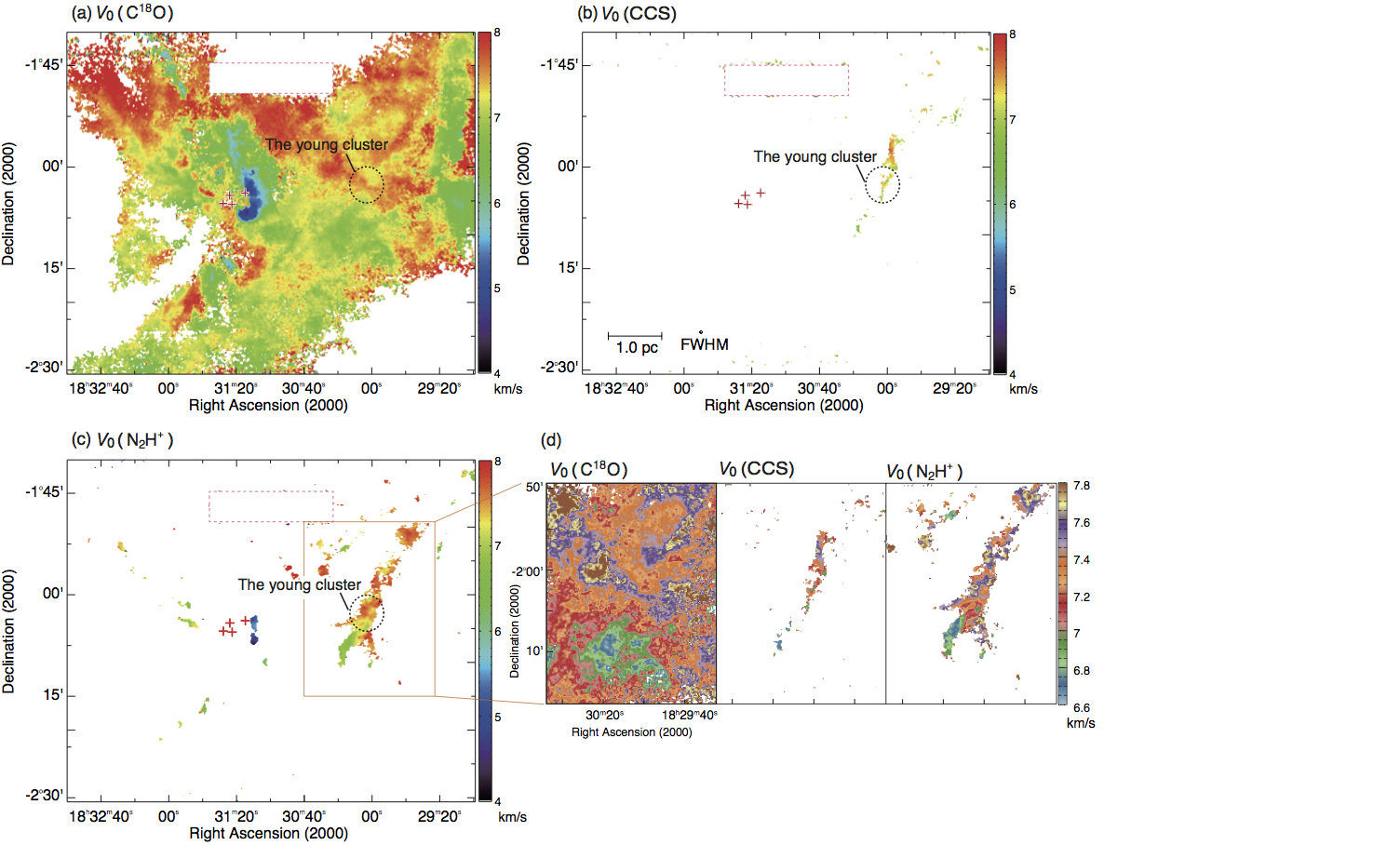
Figure 8: Mean velocity maps of the (a) C¹⁸O, (b) CCS, and (c) N₂H⁺ emission lines. The map of N₂H⁺ was obtained by fitting all of the hyperfine lines (see text). (d) Close-up view of each map for the Serpens South region.

We show the results in figures 8a and 8b. For the N₂H⁺ ($J=1-0$) line in figure 8c, we show the values of $V_{0}$ fitted with equations (1) and (2) as described in the previous subsection.

The global spatial distributions of ${V_{0}}$ of the three emission lines show a similar velocity gradient from inner regions of W40 to the Serpens South region. We found that Serpens South is accompanied by molecular gas with multiple velocity components, as reported in the previous studies for limited regions (e.g., Kirk et al., 2013; Fernández-López et al., 2014; Nakamura et al., 2014): In the southern part of Serpens South, the three emission lines are detected at $\sim 6-7$ km s^-1, while these are detected at higher velocities in the northern part.

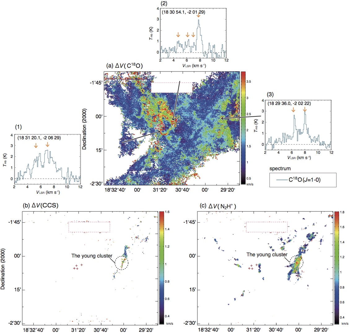
Figure 9: Velocity width (FWHM) maps of the (a) C¹⁸O, (b) CCS, and (c) N₂H⁺ emission lines. In panel (a), the C¹⁸O spectra observed at some positions indicated by the black arrows are shown. Orange arrows denote distinct velocity components seen in the spectra.

In figure 9, we also show the velocity dispersion ${\Delta V}$ maps for the three emission lines. The ${\Delta V}$ maps for the ${\rm C^{18}O}$ and CCS emission lines are derived from a single Gaussian fitting for each line profile. In the case of ${\rm C^{18}O}$ , ${\Delta V}$ is especially larger around the H ii region. The reason for the larger ${\Delta V}$ is that there are multiple velocity components as can be seen in the spectra in the figure. We also found that ${\Delta V}$ of CCS and N₂H⁺ tends to be large around the young cluster of Serpens South, which is also seen in the spectra shown in figure 7c. This is also thought to be due to the existence of multiple velocity components, as we will suggest in subsection 3.5.

3.4 The distribution of the fractional abundance

To understand chemical characteristics of the observed region, we estimated fractional abundances of ${\rm C^{18}O}$ , CCS, and N₂H⁺ . On the assumption of the LTE condition, the column density of ${\rm C^{18}O}$ and CCS, $N$(${\rm C^{18}O}$ ) and $N$(CCS), respectively, can be approximated using the integrated intensity of the lines, $\int T{\rm{}_{mb}}dv$, with the following formula (e.g., Hirahara et al., 1992; Mangum & Shirley, 2015),

$$N=\frac{3h}{8\pi^{3}}\frac{Q}{\mu^{2}S_{ij}}\frac{e^{Eu/k{T}_{\mathrm{ex}}}}{e^{T_{0}/T_{\mathrm{ex}}}-1}\frac{\int\beta^{-1}T{\rm{}_{mb}}dv}{J(T_{\mathrm{ex}})-J(T\mathrm{{}_{bg}})}$$ (4)

where $Q$ is the partition function approximated as $Q=k\,T_{\rm ex}/h\,B_{0}+1/3$ (e.g., Mangum & Shirley, 2015). $B_{0}$ is the rotational constant of the molecule. $\mu$ is the dipole moment, $E_{u}$ is the energy of the upper level, and $S_{ij}$ is the intrinsic line strength of the transition for $i$ to $j$ state. $\beta$ is the escape probability related with the optical depth $\tau$ as $\beta=(1-{e^{-\tau}})/\tau$, and $\beta=1$ for $\tau\ll 1$. For $T_{\rm ex}$, we adopted $T^{\rm{co}}_{\rm ex}$ for ${\rm C^{18}O}$ , and a fixed value of 5 K for CCS measured in dark clouds (e.g., Hirota et al., 2009). The spectral line parameters are taken from Splatalogue.

For the estimation of the column density of N₂H⁺ , $N$(N₂H⁺ ), we used the following formula (e.g., Caselli et al., 2002; Mangum & Shirley, 2015),

$$N({\rm N}_{2}{\rm H}^{+})=\frac{8\pi^{3/2}}{2\sqrt{\rm{ln}2}}\frac{Q{\nu^{3}}}{c^{3}Ag_{u}}\frac{\tau_{\rm tot}\Delta V}{1-e^{-{T_{0}/T_{\mathrm{ex}}}}}\,$$ (5)

where $g_{u}$ is the degeneracy of the upper level of a transition, $A$ is the Einstein coefficient for spontaneous emission. We calculated $Q$ using the excitation temperature $T_{\rm ex}^{\rm N_{2}H^{+}}$ derived in Section 3.2. We summarize the line parameters used in this study in table 2.

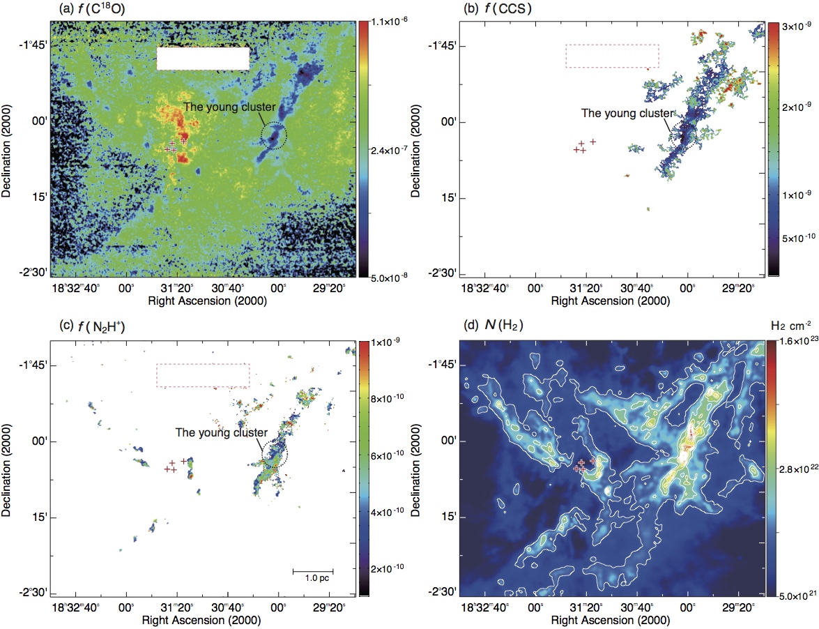
Figure 10: Fractional abundance maps of (a) C¹⁸O, (b) CCS, and (c) N₂H⁺. We also show the $N$(H₂) map (e.g., André et al., 2010) in panel (d). The lowest contour and contour interval for the $N$(H₂) map are $1\times 10^{22}$ cm^-2.

We then estimated the fractional abundances of the three molecules, $f$(${\rm C^{18}O}$ ), $f$(N₂H⁺ ), and $f$(CCS), by dividing their derived column densities by the H₂ column density derived from the dust data by $\it{Herschel}$. For this, we re-gridded and smoothed the H₂ column density data to the same angular resolution of the 45 m data ($\sim 22\arcsec$). Figure 10 shows the resultant fractional abundance maps.

The value of $f$(${\rm C^{18}O}$ ) reaches as high as $\sim 10^{-6}$ around the center of W40, but it is apparently much lower in Serpens South, which may be due to the depletion of ${\rm C^{18}O}$ onto dust in the cold and dense interior of the Serpens South filament. On the other hand, $f$(N₂H⁺ ) is high in Serpens South. $f$(CCS) is also high in Serpens South, which means that the Serpens South region is in an earlier evolutionary stage than the W40 region (e.g., Shimoikura et al., 2012, 2018). In the Serpens South region, the low values of $f$(${\rm C^{18}O}$ ), $f$(CCS), and $f$(N₂H⁺ ) are seen at the position of the young cluster. Because the difference of the fractional abundances infer the difference of chemical reaction time (e.g., Suzuki et al., 1992), the northern part of the Serpens South filament is likely to be younger than the southern part. The next cluster formation may occur in the northern part of the filament, as suggested by Nakamura et al. (2014).

3.5 The four velocity components

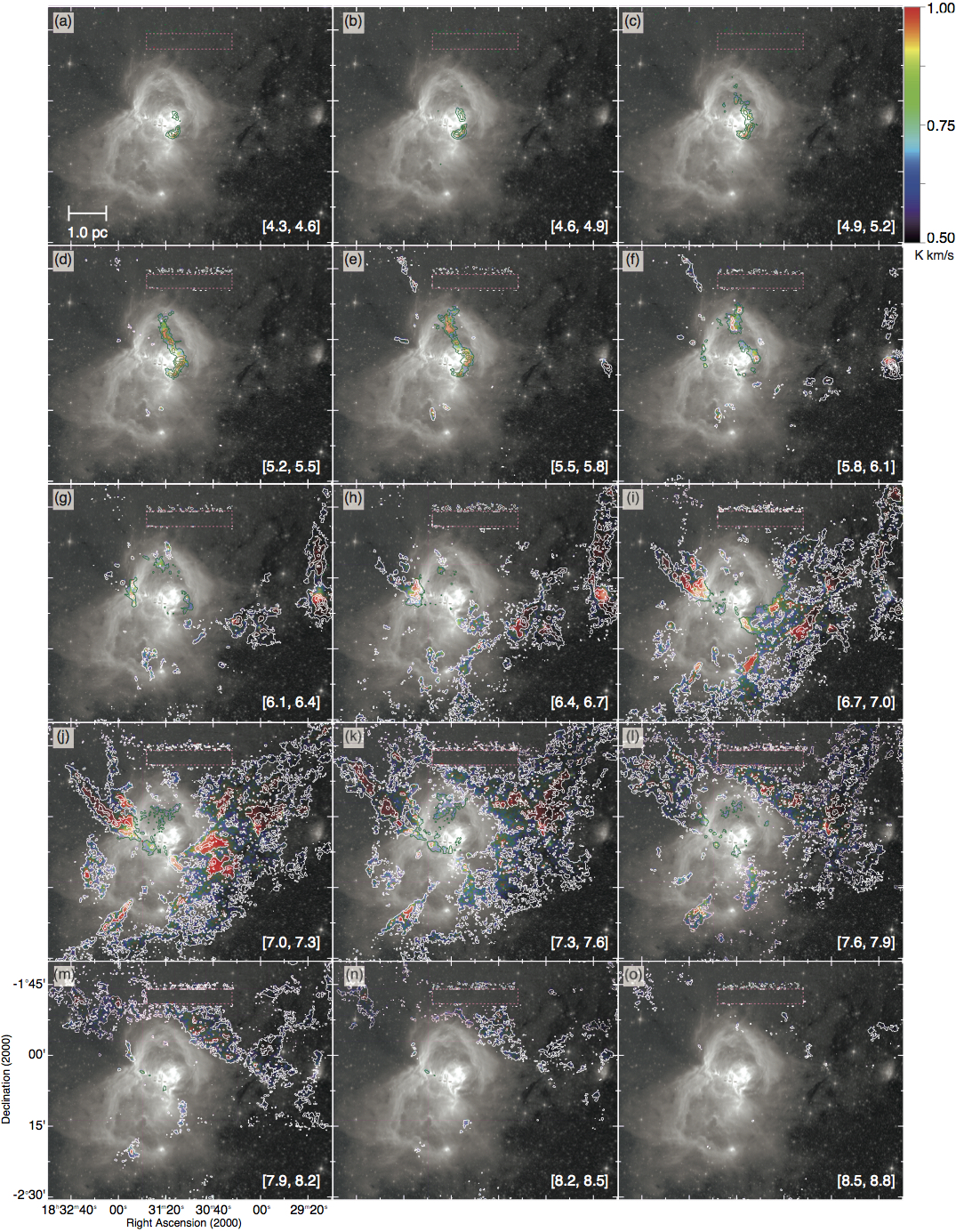
Figure 11: Channel maps of the C¹⁸O emission made at every 0.3 km s^-1 in the velocity range from 4.3 km s^-1 to 8.8 km s^-1. Each panel is overlaid on the image shown in figure 1. The velocity range (in units of km s^-1) used for the integration is shown in the brackets in each panel. The lowest contour level and the contour interval are 0.5 K km s^-1. The color scale for the C¹⁸O intensity is indicated in the top right corner.

To investigate the velocity distribution of the C¹⁸O emission in more detail and to investigate the relation between the ionization front and the molecular gas, we made channel maps of the C¹⁸O emission with a step of 0.3 km s^-1, and show them in figure 11 together with the $Spitzer$ composite image same as figure 1.

In the figure, the C¹⁸O distribution shows a complex velocity structure and varies from panel to panel. Most of the C¹⁸O emission concentrates at $\sim$ 7 km s^-1, and the emission associated with Serpens South is also found around this velocity. At low velocities in panels a $-$ e, the C¹⁸O emission is found only around the OB cluster. At higher velocities in the other panels, the emission tends to be located in the periphery of the H ii region seen in the $\it{Spitzer}$ image, for which we suggest that the C¹⁸O emission should trace the gas swept up by the expansion of the H ii region.

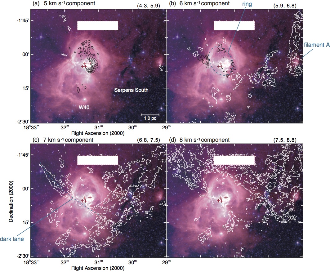
Figure 12: The ${\rm C^{18}O}$ intensity distributions of the four velocity components shown by the black/white contours (see text). The lowest contour and the contour interval are 1.4 K km s^-1. The background image is the same as that in figure 1. Velocity ranges in units of km s^-1 used for the integration of each component are shown in the parentheses above each panel.

As shown in the panels $1-3$ of figure 9, there found a number of velocity components detected in C¹⁸O in the observed region. Based on the inspection of the channel maps, we decided to categorize the emission into four groups in terms of the apparent spatial distributions around the H ii region. We shall call them 5, 6, 7, and 8 km s^-1 components according to their typical LSR velocities. These components show different features and are helpful to understand the global velocity structure of the observed region. Figure 12 shows distributions of the four components superposed on the $\it{Spitzer}$ image (figure 1). In the following, we summarize the characteristics of the components seen in figures 8 $-$ 12.

5 km s^-1 component: As seen in figure 12a, The molecular gas with LSR velocities in the range $4.3\leq V_{\rm LSR}\leq 5.9$ km s^-1 is mainly located just around the H ii region. The excitation temperature of this component is very high in the H ii region, suggesting that the component is located near the exciting sources (the OB cluster) and is warmed by the radiation from them.

6 km s^-1 component: As seen in figure 12b, the molecular gas with LSR velocities $5.9\leq V_{\rm LSR}\leq 6.8$ km s^-1 are found around the H ii region and at the southern part of the main body of Serpens South. The component located around the H ii region shows a ring-like structure surrounding the 5 km s^-1 component. In addition, there is a filament at $\sim 6$ km s^-1 with an elongation of $\sim 3$ pc at the most western side in the observed area (as labelled “filament A”). This filament shows an anti-correlation with the 8 km s^-1 component shown in figure 12d.

7 km s^-1 component: As seen in figure 12c, the molecular gas with LSR velocities in the range $6.8\lesssim V_{\rm LSR}\lesssim 7.5$ km s^-1 are found mainly around the Serpens South region as well as in the periphery of the H ii region. The diffuse and extended emission is also detected in the H ii region, being coincident with the dark lane. The component associated with the dark lane is extending from the Serpens South region to the W40 region, as traced by the broken line.

8 km s^-1 component: As seen in figure 12d, the molecular gas with LSR velocities in the range $7.5\lesssim V_{\rm LSR}\lesssim 8.8$ km s^-1 appears to lie at the boundary of the H ii region. The component is seen mostly in the north-western side of the H ii region.

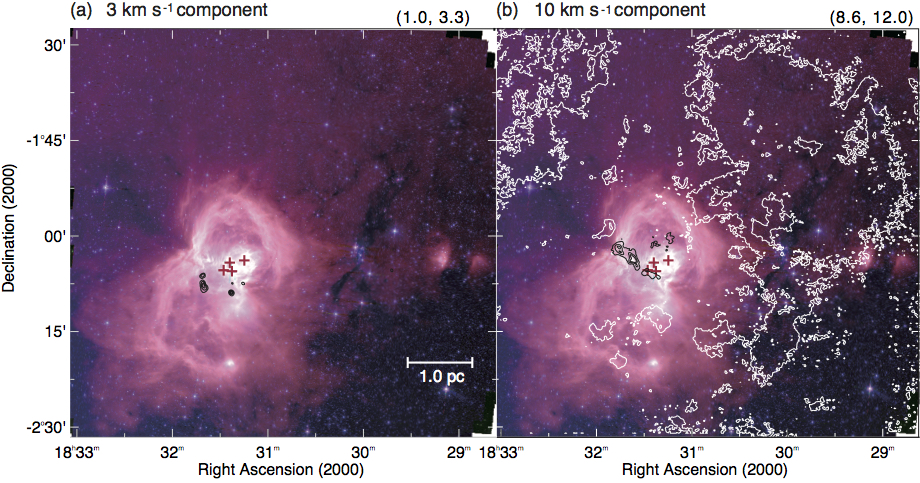
Figure 13: Distributions of the 3 km s^-1 component and the 10 km s^-1 component identified based on the ¹³CO data (see text). Velocity ranges in units of km s^-1 used for the integration of each component are shown in the parentheses above each panel. The lowest contour and the contour interval are 3.0 K. The background images are the same as that in figure 1.

In our previous study using the ¹²CO ($J=3-2$) and HCO⁺ ($J=4-3$) emission lines performed only in the limited region around the W40 H ii region, we reported that there are velocity components at $V_{\rm LSR}\simeq 3$, 5, 7, and 10 km s^-1 (Shimoikura et al., 2015). These velocity components are mostly single peaked components with well-defined radial velocities and are not categorized in the same way as the four components in the above, but the 5 and 7 km s^-1 components found in the previous study can be merged into those categorized in this work. The $\sim 3$ and $\sim 10$ km s^-1 components found in the previous work are not detected in ${\rm C^{18}O}$ in this study with a good signal-to-noise ratio. However, they are clearly detected in the ¹²CO ($J=1-0$) and ¹³CO ($J=1-0$) lines. In figure 13, we show the distributions of the $\sim 3$ and $\sim 10$ km s^-1 components detected in the ¹³CO ($J=1-0$) data, and we shall call them the 3 and 10 km s^-1 component, respectively. These components are seen around the OB cluster as we already found in the earlier study. In this study, we further found that the 10 km s^-1 component is widely distributed over the observed area, especially in the periphery of the H ii region like the 8 km s^-1 component in figure 12d.

In summary, the distributions of the identified components indicate an interaction between the H ii region and the surrounding molecular gas. The components at higher velocities (i.e., 7, 8, and 10 km s^-1) tend to exhibit an arc-shaped structure and are located at the boundary of the H ii region, suggesting that they may be tracing expanding shell of the H ii region.

3.6 The two expanding shells

To better understand the spatial and velocity distributions of molecular gas and to investigate the effect of the expanding H ii region on the surroundings, we made position-velocity (PV) diagrams across the observed region using the ${\rm C^{18}O}$ data. Figure 14 displays a series of the PV diagrams measured along the cuts centered at the position of IRS1A South toward various directions. In each PV diagram, the position of IRS1A South as well as the positions separated by $\pm 1000\arcsec$ away from the source roughly corresponding to the boundary of the H ii region are indicated by the white broken lines.

We found elliptical structures in the diagrams as we indicate two of them by ellipses in panels i and p where the structures are evident. The elliptical structures should be due to expanding shell(s) of the H ii region centered at IRS1A South or the OB cluster. We suggest that there are two shell-like structures: One is the small inner shell just around IRS1A South shown by the ellipse in panel p, and the other is the large outer shell corresponding to the boundary of the H ii region delineated by the ellipse in panel i. The ellipses in the panels indicate that the inner and outer shells have a radius of $\sim 0.5$ pc and $\sim 2.5$ pc, and an expanding velocity of $\sim 3$ km s^-1. The expansion time scale of the two shells can be estimated by dividing the radius by the velocity to be $1.6\times 10^{5}$ yr and $8.1\times 10^{5}$ yr for the inner and outer shells, respectively, which is consistent with the dynamical age of the H ii region ($1.9\times 10^{5}-7.8\times 10^{5}$ yr) estimated by Mallick et al. (2013) based on the radio continuum observations. We also estimated the mass within the outer shell (the northwest side of the W40 region) to be $\sim 1\times 10^{3}M_{\odot}$.

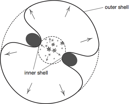
Figure 15: A schematic representation of the W40 H ii region showing that the two shells were created by the expansion of the H ii region. The small inner shell is found in the vicinity of the H ii region, and the other is the larger outer shell corresponding to the boundary of the H ii region.

We suggest a possibility that the two shell-like structures were created due to the inhomogeneous density distribution of the dense gas around the H ii region. As seen in figure 12, there are some patchy dense clumps (e.g., the $5-7$ km s^-1 components) in the vicinity of IRS 1 A South and the OB cluster. Expansion of the H ii region should be slowed or blocked by such clumps, and some parts of the expanding shell facing to the clumps should appear as the inner shell, while the rest of the shell should appear as the outer shell, as illustrated in figure 15. We further suggest that this may be the very mechanism to create the hourglass-shaped structure of the H ii region.

3.7 The cluster formation in Serpens South

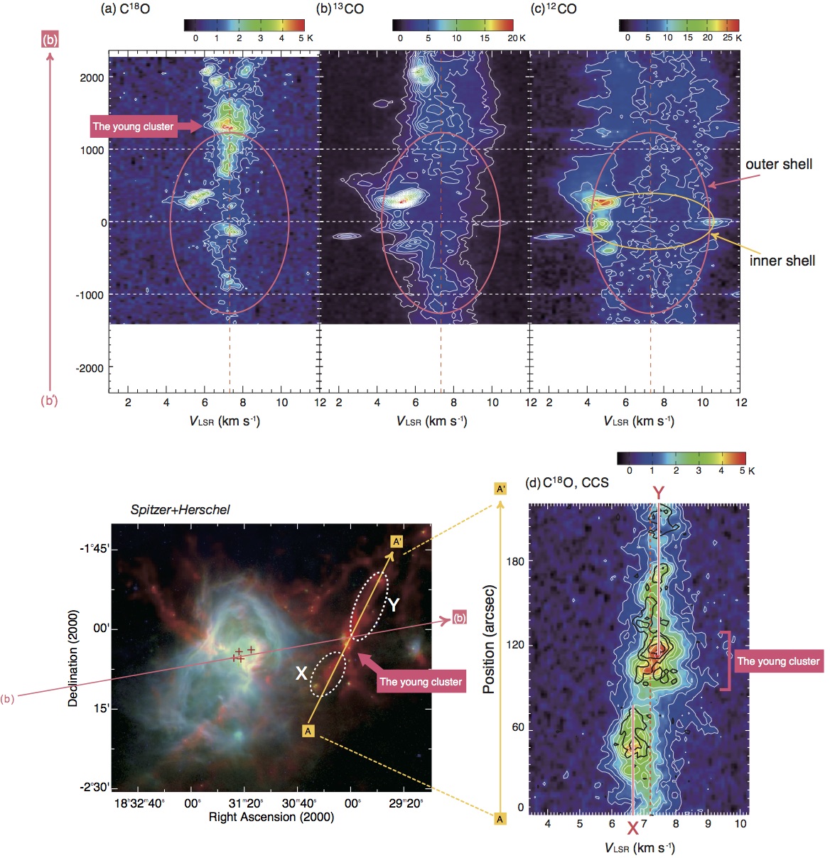
Figure 16: (a) PV diagram of the ${\rm C^{18}O}$ emission line (the same diagram as figure 14b). PV diagram of (b) the ¹³CO emission line and (c) the ¹²CO emission line taken along the same cut labeled b’-b. The lowest contour and contour interval are 1.0 K km s^-1 for panel (b) and 4.0 K km s^-1 for panel (c). (d) PV diagram of the C¹⁸O emission line (color scale + white contour) and CCS emission line (black contour) taken along the cut A-A’. The lowest contour and contour interval are 0.6 K km s^-1 for ${\rm C^{18}O}$ and 0.4 K for CCS. The vertical broken line indicates the systemic velocity ($V_{\rm LSR}=7.3$ km s^-1) for panes a – d.

We investigated whether the expansion of the H ii region influenced the cluster formation in Serpens South. Figure 16a (same as figure 14b) shows the PV diagram measured along the cut b’-b crossing the position of the young cluster of Serpens South. The outer shell delineated by the ellipse in figure 16a is not seen very well in the ${\rm C^{18}O}$ emission, so we show in figures 16b and c the PV diagrams of the ¹³CO and ¹²CO emission taken along the same cut, respectively, where the outer shell can be better recognized. As seen in the PV diagrams, the dense gas associated with the young cluster (evident in figure 16a) is very likely to be located at the surface of the outer shell, indicating that the natal clump of the cluster can be affected by the shell. Actually, as seen in figure 16a, the velocity dispersion is enhanced abruptly at the position of the cluster (up to $\sim 2$ km s^-1) compared to the adjacent positions, which can be recognized also in the ${\Delta V}$ maps presented in figures 9b and c. Though the observed enhancement of the velocity dispersion may be partially due to the feedback of star formation (e.g., outflows), this may support the idea that the natal clump of the young cluster is interacting with the outer shell being compressed by the expansion of the shell, which may have induced the formation of the young cluster.

To further investigate the influence of the outer shell, we created a PV diagram for the C¹⁸O and CCS emission along the major axis of the Serpens South filament, which is shown in figure 16d. In the figure, there can be found two major velocity components as labeled “X” and “Y” which correspond to subfilaments extending to the southeast and northwest, respectively. The subfilament X has a velocity ($\sim 6$ km s^-1) slightly lower than the systemic velocity ($\sim 7$ km s^-1), and the subfilament Y has a velocity same as the systemic velocity. The young cluster is apparently located at the intersection of the subfilaments X and Y, and both of them are located around the surface of the outer shell. This positional coincidence infers a scenario that the subfilament X has been accelerated by the expansion of the outer shell and recently collided against the subfilament Y to induce cluster formation at the intersection.

The previous studies (e.g., Kirk et al., 2013; Nakamura et al., 2014) also reported that Serpens South consists of molecular filaments with different velocities. Nakamura et al. (2014) suggested that the collisions of the filaments with the different radial velocities may have triggered the cluster formation like what we discuss in the present study. The PV diagram of figure 16d shows a velocity gradient from southeast to northwest of $\sim 0.7$ km s^-1 pc^-1, which is consistent with that found by the previous studies (Kirk et al., 2013; Fernández-López et al., 2014). Kirk et al. (2013) interpreted that the velocity gradient is an evidence of material flowing inside the filaments, leading to infall toward the intersection of the filaments where the cluster formation takes place. However, Fernández-López et al. (2014) suggest that the velocity gradients can also occur in scenarios where filaments are created by large-scale turbulence.

We basically agree with the scenario suggested by Nakamura et al. (2014) that the cluster formation was induced by collisions of filaments. Our subfilaments X and Y correspond to their filaments F8 and F1-3, respectively (see their figure 3). We further suggest that the outer shell of the W40 H ii region have played a crucial role to accelerate the southeastern part of the filament (i.e., the subfilament X) leading to the collisions of the filaments. Also, the outer shell may have influenced directly on the natal clump of the cluster by compressing it to trigger the cluster formation.

3.8 The global 3D structure

In our previous work (Shimoikura et al., 2015), we investigated the three-dimensional structure of W40 just around the H ii region. Because we are now almost confident that W40 and Serpens South belong to the same system, we will try to investigate the three-dimensional structure of the entire system based on the data obtained in this study.

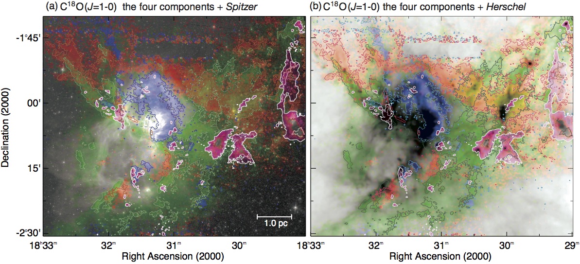
Figure 17: Composite color image of W40 and Serpens South made from the integrated intensity maps, with the 5 km s^-1 component in blue, the 6 km s^-1 component in pink, and the 7 km s^-1 component in green, and the 8 km s^-1 component in red, respectively. The background image is the same as that in figure 1 for panel (a), and the $\it{Herschel}$ 250$\micron$ image for panel (b).

In figure 17, we present the spatial distributions of each component together with the IR images. Considering the velocity difference of each component with respect to the systemic velocity at 7 km s^-1 as well as the expanding motion of the H ii region, the W40 + Serpens South system should be structured basically in such a way that the 5 km s^-1 and 6 km s^-1 components are located on the near side of the H ii region facing toward us, and the 8 km s^-1 component is located on the far side.

Based on the above picture, we attempt to reveal the locations of the individual components in the system. The 5 km s^-1 component is distributed only around the center of the H ii region. It must be the dense gas close to and being blown away by the H ii region, and moving toward us. This component is probably located at the inner shell. The 6 km s^-1 component and a part of the 7 km s^-1 component seen around the main body of Serpens South appear as the absorption (i.e., dark) in the $\it{Spitzer}$ image, delineating the shape of the Serpens South filaments. The absorption indicates that they must be the dense gas located in the foreground of the H ii region. The dark lane located in the waist of the H ii region at 7 km s^-1 also obscures the central part of the H ii region in the $\it{Spitzer}$ image, and therefore it must be located in the foreground. The 8 km s^-1 component is found mainly in the northern part of the observed region, and it does not appear as the absorption in the $\it{Spitzer}$ image, suggesting that it is located rather in the back of the H ii region.

We further attempt to model the locations of the 3 and 10 km s^-1 components identified with the ¹³CO data in the same way. We found a high temperature of $\sim 30$ K for the components as seen in figure 6a, suggesting that they are located close to the central OB stars. As seen in the PV diagram of figure 16c, the 10 km s^-1 component is apparently located at the inner shell of the H ii region on the far side to the observer, which is consistent with the suggestion in our previous study (Shimoikura et al., 2015). The 3 km s^-1 component is also likely to be located at the inner shell but on the near side to the observer, like in the case of the 5 km s^-1 component.

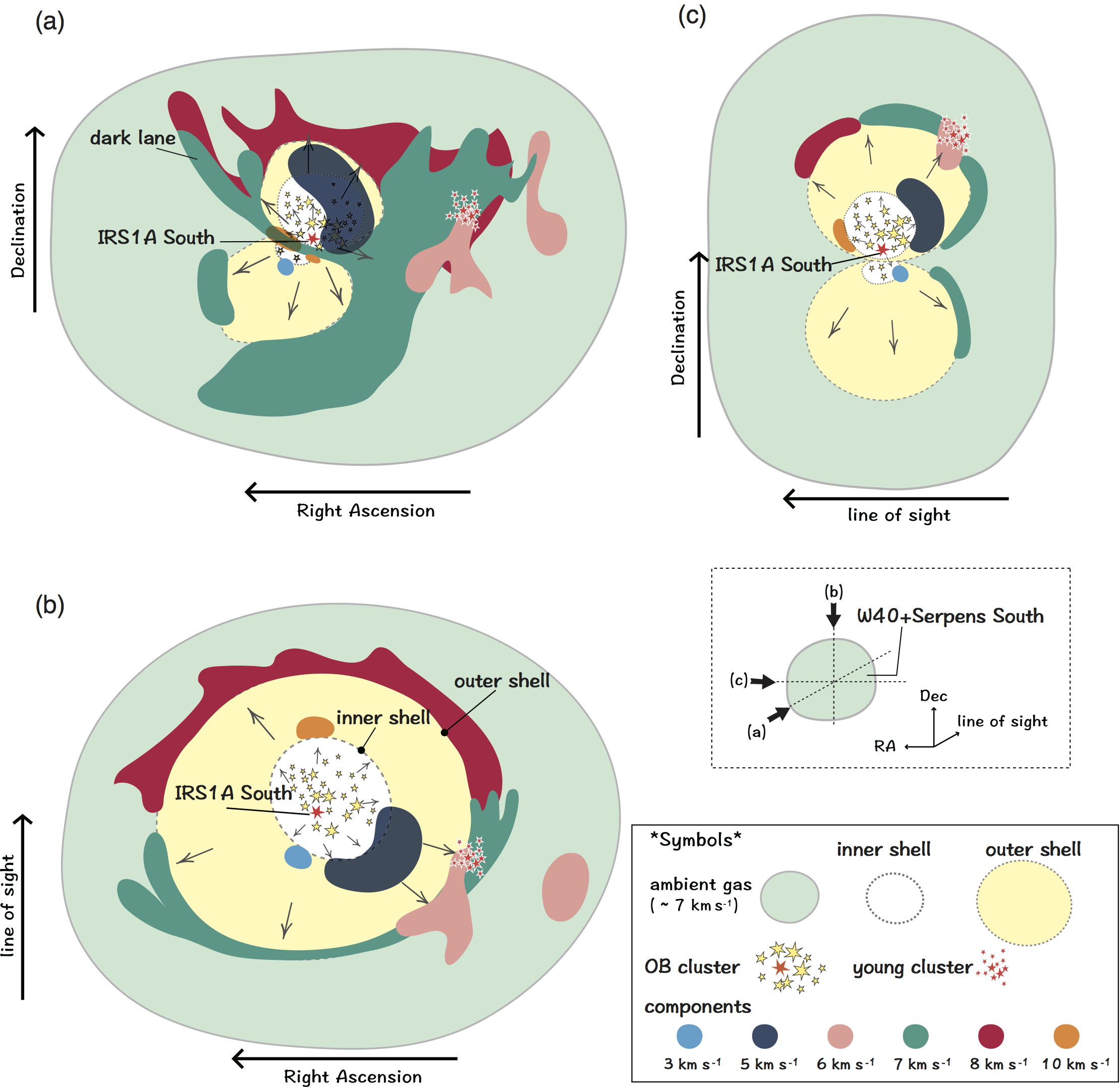
Figure 18: Schematic illustration of the proposed model for the three-dimensional geometry of the W40 and Serpens South complex. As indicated in the box drawn by the broken line, panel (a) shows the view as is observed on the sky (e.g., see figure 17), panel (b) shows the view observed from the declination axis orthogonal to the line of sight, and panel (c) shows the view observed from the right ascension axis. There are two expanding shells created by the H ii region (see figure15). In the model, the 3 and 5 km s^-1 components are located on the near side of the inner shell, and the 10 km s^-1 component is located on the far side of the inner shell. The 6 and 7 km s^-1 component are located around the surface of the outer shell. Both of the components associated with the young cluster of Serpens South are likely to be interacting with the outer shell. The 8 km s^-1 component is located on the far side of the outer shell.

In figure 18, we summarize the geometry of the entire W40 and Serpens South system inferred from the above discussion. The morphology and kinematics around the W40 H ii region are consistent with what we proposed before (Shimoikura et al., 2015). Finally, using the $\it{Herschel}$-based $N$(H₂) data, we estimated the total mass of the four components to be $\sim 200$, $\sim 1200$, $\sim 5000$, and $\sim 2000M_{\odot}$ for the 5, 6, 7, and 8 km s^-1 component, respectively.

As seen in the PV diagrams (figure 14), the velocity distribution of each component is narrow with a line width of $\sim 1$ km s^-1, except for the 5 km s^-1 component. According to Beaumont & Williams (2010) who observed 43 bubbles associated with H ii regions, there is often a ring of cold gas driven by massive stars, and H ii regions form in flat molecular clouds with a thickness of a few parsecs. We point out a possibility that some filamentary structures seen around the equator of the hourglass-shaped W40 H ii region can be an edge-on view of a sheet-like or ring-like cloud, like what was suggested by Beaumont & Williams (2010) for other H ii regions.

In general, as an advancing ionization front wraps pre-existing clumps, its pressure triggers a gravitational collapse and star formation (e.g., Elmegreen & Lada, 1977). The two shells we found in this study have apparently been created by the H ii region, and they may be such a place of sequential star formation, as it is actually evident in figure 5 showing the distributions of YSOs (André et al., 2010; Könyves et al., 2015). In the W40 and Serpens South system, star formation probably occurred in W40 first, and then the next-generation stars are forming in clouds along the expanding shells. We suggest that the young cluster in Serpens South was also induced by the expansion of the H ii region. This idea is consistent with the fact that the CCS emission is strongly detected in the Serpens South region while it is not detected in W40, indicating that the Serpens South region is much younger than the W40 region.

4 CONCLUSIONS

Large-scale mapping observations of the star-forming regions of W40 and Serpens South were performed in ¹²CO, ¹³CO, C¹⁸O, CCS, and N₂H⁺ using the NRO 45 m telescope. We revealed the complex distributions of the molecular emission lines and their radial velocities in the regions. We found that the C¹⁸O emission is smoothly distributed over the both W40 and Serpens South regions, suggesting that the two regions belong to the same system. The CCS and N₂H⁺ emission lines are enhanced in Serpens South. Serpens South is characterized by its filamentary structure in the infrared images such as by $Spitzer$ and $Hershell$, and it is accompanied by a young cluster near the center of the structure. On the other hand, in W40, the CCS emission is not detected significantly, and the N₂H⁺ emission is detected almost only around an OB cluster at the center.

Based on the C¹⁸O observations, we divided the molecular gas into four velocity components which we call 5, 6, 7, and 8 km s^-1 components according to their typical LSR velocities. We found that two elliptical structures are seen in the position-velocity diagrams, which can be explained as a part of two expanding shells. One of these shells is the small inner shell found in the vicinity of the H ii region, and the other is the larger outer shell corresponding to the boundary of the H ii region. The dense gas associated with the young cluster in Serpens South is likely to be interacting with the outer shell, for which we suggest that the cluster was induced to form by the interaction with the expanding outer shell.

Strong CCS emission is detected in Serpens South while it is not detected in W40, which means that the Serpens South region is younger than the W40 region in terms of chemical reaction. This result is consistent with the scenario that the star formation initially occurred in W40 and then the young cluster in Serpens South was induced to form by the interaction with the expanding shell of the H ii region.

Based on the morphologies and velocity distributions of the four velocity components as well as their appearance in the infrared images, we made a three-dimensional geometrical model of the W40 and Serpens South regions.

We are grateful to the referee for providing useful comments to improve this paper. We thank Yoshiko Hatano, Akifumi Yamabi, Sho Katakura, and Asha Hirose for their support of the observations. We are also grateful to the other members of Star Formation Legacy project. This work was supported by JSPS KAKENHI Grant Numbers JP17K00963, JP17H02863, JP17H01118, JP16K12749. YS received support from the ANR (project NIKA2SKY, grant agreement ANR-15-CE31-0017). The 45 m radio telescope is operated by NRO, a branch of NAOJ. This research has made use of data from the Herschel Gould Belt survey (HGBS) project (http://gouldbelt-herschel.cea.fr). The HGBS is a Herschel Key Programme jointly carried out by SPIRE Specialist Astronomy Group 3 (SAG 3), scientists of several institutes in the PACS Consortium (CEA Saclay, INAF-IFSI Rome and INAF-Arcetri, KU Leuven, MPIA Heidelberg), and scientists of the Herschel Science Center (HSC).

Table 1: The observed molecular lines

Molecule	Transition	Frequency	Effective beam size	$\Delta T_{\rm mb}$
		(GHz)	($\arcsec$)	(K)
N2H+	$J=1-0$	93.1737637	$24$	0.27
CCS	$J_{N}$=8${}_{7}-7_{6}$	93.8700980	$24$	0.26
C18O	$J=1-0$	109.7821760	$22$	0.33
13CO	$J=1-0$	110.2013540	$22$	0.36
12CO	$J=1-0$	115.2712040	$22$	0.87

The rest frequency for the N₂H⁺ line is taken from Pagani et al. (2009), and those of the other lines are taken from the website of Lovas (1992).
The one sigma noise level at a velocity resolution of 0.1 km s^-1.

Table 2: Constants of the observed molecular lines

Molecule	Transition	$S_{ij}$	$B_{0}$	$\mu$	$E_{u}$	$g_{u}$	$A$
			(GHz)	(Debye)	(cm-1)		($s^{-1}$)
N2H+	$J=1-0$	-	46.586867	-	-	3	3.628$\times$10-5
CCS	$J_{N}$=8${}_{7}-7_{6}$	7.97	6.47775036	2.88	13.82557	-	-
C18O	$J=1-0$	1.00	54.8914	0.110	3.66194	-	-

Pagani et al. (2009)

References

- André et al. (2010) André, P., et al. 2010, A&A, 518, L102
- Beaumont & Williams (2010) Beaumont, C. N., & Williams, J. P. 2010, ApJ, 709, 791
- Bontemps et al. (2010) Bontemps, S., et al. 2010, A&A, 518, L85
- Caselli et al. (2002) Caselli, P., Benson, P. J., Myers, P. C., & Tafalla, M. 2002, ApJ, 572, 238
- Caselli et al. (1995) Caselli, P., Myers, P. C., & Thaddeus, P. 1995, ApJ, 455, L77
- Dobashi (2011) Dobashi, K. 2011, PASJ, 63, 1
- Dobashi et al. (2005) Dobashi, K., Uehara, H., Kandori, R., Sakurai, T., Kaiden, M., Umemoto, T., & Sato, F. 2005, PASJ, 57, 1
- Elmegreen & Lada (1977) Elmegreen, B. G., & Lada, C. J. 1977, ApJ, 214, 725
- Fernández-López et al. (2014) Fernández-López, M., et al. 2014, ApJ, 790, L19
- Friesen et al. (2013) Friesen, R. K., Medeiros, L., Schnee, S., Bourke, T. L., di Francesco, J., Gutermuth, R., & Myers P. C. 2013, MNRAS, 436, 1513
- Gutermuth et al. (2008) Gutermuth, R. A., et al. 2008, ApJ, 673, L151
- Hirahara et al. (1992) Hirahara, Y., et al. 1992, ApJ, 394, 539
- Hirota et al. (2009) Hirota, T., Ohishi, M., & Yamamoto, S. 2009, ApJ, 699, 585
- Kirk et al. (2013) Kirk, H., Myers, P. C., Bourke, T. L., Gutermuth, R. A., Hedden, A., & Wilson, G. R.2013, ApJ, 766, 115
- Könyves et al. (2010) Könyves, V., et al. 2010, A&A, 518, L106
- Könyves et al. (2015) Könyves, V., et al. 2015, A&A, 584, A91
- Kuhn et al. (2010) Kuhn, M. A., Getman, K. V., Feigelson, E. D., Reipurth, Bo., Rodney, S. A., & Garmire G. P. 2010, ApJ, 725, 2485
- Kutner & Ulich (1981) Kutner, M. L., & Ulich, B. L. 1981, ApJ, 250, 341
- Lee et al. (2004) Lee, J., Bergin, E. A., & Evans II, N. J. 2004, ApJ, 617, 360.
- Lovas (1992) Lovas, F. J. 1992, Journal of Physical and Chemical Reference Data, 21, 181
- Mallick et al. (2013) Mallick, K. K., Kumar, M. S. N., Ojha, D. K., Bachiller, R., Samal, M. R., & Pirogov, L. 2013, ApJ, 779, 113
- Mangum & Shirley (2015) Mangum, J. G., & Shirley, Y. L. 2015, PASP, 127, 266
- Maury et al. (2011) Maury, A. J., André, P., Men’shchikov, A., Könyves, V., & Bontemps, S. 2011, A&A, 535, A77
- Minamidani et al. (2016) Minamidani, T., et al. 2016, in Proc. SPIE, Vol. 9914, Millimeter, Submillimeter, and Far-Infrared Detectors and Instrumentation for Astronomy VIII, 99141Z
- Nakamura et al. (2017) Nakamura, F., Dobashi, K., Shimoikura, T., Tanaka, T., & Onishi, T. 2017, ApJ, 837, 154
- Nakamura et al. (2011) Nakamura, F., Sugitani, K., Shimajiri, Y., et al. 2011, The Astrophysical Journal, 737, 56.
- Nakamura et al. (2014) Nakamura, F., et al. 2014, ApJ, 791, L23
- Ortiz-León et al. (2017) Ortiz-León, G. N., et al. 2017, ApJ, 834, 143
- Pagani et al. (2009) Pagani, L., Daniel, F., & Dubernet, M.-L. 2009, A&A, 494, 719
- Pirogov et al. (2013) Pirogov, L., Ojha, D. K., Thomasson, M., Wu, Y.-F., & Zinchenko, I. 2013, MNRAS, 436, 3186
- Rodney & Reipurth (2008) Rodney, S. A., & Reipurth, B. 2008, The W40 Cloud Complex, ed. B. Reipurth (San Francisco, CA: ASP), 683
- Rumble et al. (2016) Rumble, D., et al. 2016, MNRAS, 460, 4150
- Sawada et al. (2008) Sawada, T., et al. 2008, PASJ, 60, 445
- Shimajiri et al. (2017) Shimajiri, Y., et al. 2017, A&A, 604, A74
- Shimoikura et al. (2015) Shimoikura, T., Dobashi, K., Nakamura, F., Hara, C., Tanaka, T., Shimajiri, Y., Sugitani, K., & Kawabe, R. 2015, ApJ, 806, 201
- Shimoikura et al. (2012) Shimoikura, T., Dobashi, K., Sakurai, T., Takano, S., Nishiura, S., & Hirota, T. 2012, ApJ, 745, 195
- Shimoikura et al. (2018) Shimoikura, T., Dobashi, K., Nakamura, F., Matsumoto, T., & Hirota, T. 2018, ApJ, 855, 45
- Shuping et al. (2012) Shuping, R. Y., Vacca, W. D., Kassis, M., & Yu, K. C. 2012, AJ, 144, 116
- Smith et al. (1985) Smith, J., Bentley, A., Castelaz, M., Gehrz, R. D., Grasdalen, G. R., & Hackwell, J. A. 1985, ApJ, 291, 571
- Sugitani et al. (2011) Sugitani, K., Nakamura, F., Watanabe, M., et al. 2011, ApJ, 734, 63
- Suzuki et al. (1992) Suzuki, H., Yamamoto, S., Ohishi, M., Kaifu, N., Ishikawa, S., Hirahara, Y., & Takano, S. 1992, ApJ, 392, 551
- Tiné et al. (2000) Tiné, S., Roueff, E., Falgarone, E., Gerin, M., & Pineau des Forêts, G. 2000, A&A, 356, 1039
- Vallee (1987) Vallee, J. P. 1987, A&A, 178, 237