Stochastic Second-order Methods for Non-convex Optimization with Inexact Hessian and Gradient

Abstract

Trust region and cubic regularization methods have demonstrated good performance in small scale non-convex optimization, showing the ability to escape from saddle points. Each iteration of these methods involves computation of gradient, Hessian and function value in order to obtain search direction and adjust the radius or cubic regularization parameter. However, exactly computing those quantities are too expensive in large-scale problems such as training deep networks. In this paper, we study a family of stochastic trust region and cubic regularization methods when gradient, Hessian and function values are computed inexactly, and show the iteration complexity to achieve $\epsilon$-approximate second-order optimality is in the same order with previous work for which gradient and function values are computed exactly. The mild conditions on inexactness can be achieved in finite-sum minimization using random sampling. We show the algorithm performs well on training convolutional neural networks compared with previous second-order methods.

1 introduction

In this paper, we consider the unconstrained optimization problem:

$$\mathop{\min}\limits_{x\in{\mathbb{R}^{d}}}f(x)=\frac{1}{n}\sum\limits_{i=1}^{n}{{f_{i}}(x)},$$ (1)

where $f_{i}(x)$ is smooth and not necessarily convex. Such finite-sum structure is increasingly popular in modern machine learning tasks, especially in deep learning, where each $f_{i}(\cdot)$ corresponds to the loss of a training sample. For large-scale problems, computing the full gradient and Hessian is prohibitive, so Stochastic gradient descent (SGD) has become the most popular method. First order methods such as gradient descent and SGD are guaranteed to converge to stationary points, which can be a saddle point or a local minimum.

It is known that second-order methods, by utilizing the Hessian information, can more easily escape from saddle points. At each iteration, second-order methods typically build a quadratic approximation function around the current solution $x_{k}$ by

$${m_{k}}(s)=f({{x_{k}}})+\langle{{g(x_{k})},s}\rangle+\frac{1}{2}\langle{s,{B(x_{k})}s}\rangle,$$ (2)

where $g(x_{k})$ is the approximated gradient and $B(x_{k})$ is the symmetric matrix. To update the current solution, a common strategy is to minimize this quadratic approximation within a small region. Algorithms based on this idea including Trust Region method (TR) [3] and Adaptive Regularization using Cubics (ARC) [4, 5] have demonstrated good performance on small-scale non-convex problems.

However, for large-scale optimization such as training deep neural networks, it is impossible to compute gradient and Hessian exactly for every update. As a result, stochastic second-order methods have been studied in the past few years. [6, 7] proposed TR and ARC methods with inexact Hessian, in which the second-order information is approximated by the subsampled Hessian matrix, yet the gradient is still computed exactly. [8] proposed a stochastic version of ARC, but they require a much stronger condition in both gradient and Hessian approximation, thus they need to keep increasing the sample size as iteration goes. More recently, [9] provide stochastic cubic regularization method, but they do not have an adaptive way to adjust the regularization parameters.

In this paper, we consider a simple and practical stochastic version of trust region and cubic regularization methods (denoted as STR and SARC respectively). In the quadratic approximation (2), we replace both $g(x_{k})$ and $B(x_{k})$ by the approximate gradient and Hessian with a fixed approximation error, which can be achieved using a fixed sample size. Furthermore, we consider the most general case where the trust region radius or cubic regularization parameter is adaptively adjusted by checking the subsampled objective function value.

Note that we do not claim STR and SARC are “new” algorithms, since it is natural to transform TR and ARC to the stochastic setting. The question is whether this simple idea works in theory and in practice, and our contribution is to provide an affirmative answer to this question. Our contribution can be summarized as follows:

• We provide a theoretical analysis of convergence and iteration complexity for STR and SARC. Unlike [8], we do not require the approximation error of Hessian and gradient estimation to be related to $s$ (the update step). Furthermore, even though the proof framework is similar to [7], we provide novel analysis to model the case when both gradient and Hessian are inexact, while [7] does not allow inexact gradient.

• We use the operator-Bernstein inequality to bound the sub-sampled function value, which enables automatically adjusting trust region radius and cubic regularization parameter using subsamples. Even when function value, gradient and Hessian are all inexact, we are able to show that the iteration complexity is in the same order with [7, 8].

• We conduct experiments on CIFAR-10 data with VGG network and show that the proposed algorithms are faster than the existing trust region and cubic regularization methods in terms of running time.

1.1 Our results

We present the iteration complexity for both proposed methods under the Assumptions in Preliminary where the parameters are defined as well.

STR The total number of iterations is $\mathcal{O}(\max\{(\varepsilon_{\nabla f}-\varepsilon_{g})^{-2},(\varepsilon_{H}-\varepsilon_{B})^{-3}\})$.

SARC The iteration complexity is the same order of STR. If the condition of the terminal criterion is satisfied, then the total number of iterations is

$$\mathcal{O}(\max\{(\varepsilon_{\nabla f}-\varepsilon_{g})^{-3/2},(\varepsilon_{H}-\varepsilon_{B})^{-3}\}),$$

which is better than STR.

1.2 Related Work

With the increasing size of data and model, stochastic optimization becomes more and more popular since computing the gradient and Hessian are prohibitively expensive.

For the stochastic first-order optimization, stochastic gradient descent (SGD) [10, 11, 12] is absolutely the main method especially in training deep neural networks and other large-scale machine learning problems, due to its simplicity and effectiveness. However, the estimated gradient will induce the noise such that the variance of the gradient may not approximate zero even when converged to a stationary point. Stochastic variance reduction gradient (SVRG) [13] and SGAG [14] are two typical methods to reduce the variance of the gradient estimator, which lead to faster convergence especially in the convex setting. Several other related variance reduction methods are developed and analyzed for non-covex problems [15, 16]. However, using only first-order information, the saddle point may not be escaped even though [17] prove that SGD with noise can escape but under certain conditions.

For second-order optimization, Newton-typed methods rely on building a quadratic approximation around the current solution, and by exploring the curvature information it can better avoid saddle points in non-convex optimization. The negative eigenvector of the Hessian information provides the decrease direction for the updates. Using exact Hessian is often time consuming, so Broyden-Fletcher-Goldfarb-Shanno (BFGS) and Limited-BFGS [18] are two widely methods that approximate Hessian using first-order information. Another important technique for Hessian approximation is sub-sampling the function $f_{i}(\cdot)$ to obtain the estimated Hessian. Both [19] and [20] using the stochastic Hessian matrix to obtain the global convergence, while the former requires $f_{i}$ to be smooth and strongly convex. Furthermore, [21, 22] apply the sub-sampled gradient and Hessian to the quadratic model and give the convergence analysis of second-order methods thoroughly and quantitatively.

Trust region Newton method is a classical second-order method that searches the update direction only within a trust region around the current point. The size of trust region is critical to the effectiveness of search direction. The region will be updated based on measuring whether the quadratic approximation is an adequate representation of the function or not. Following the sub-sampling for Hessian matrix as in [21, 22], [6, 7] apply such inexact Hessian to trust region method and also provide the convergence and iteration complexity. Similar to the trust region method, [4, 5] introduced adaptive cubic regularization methods for unconstrained optimization, in which the Hessian metrics can be replaced by the approximate matrix. [8] apply the operator-Bernstein inequality to approximate the Hessian matrix and gradient into a quadratic function with cubic regularization. However, the sample approximate condition is subject to the search direction $s$, thus they need to increase the sample size at each step. To overcome this issue, [6] provide another approximation condition of Hessian matrix that does not depend on the search step $s$. However, they assume gradient has to be computed exactly, which is not feasible in large-scale applications. Furthermore, each update of the $\rho$ that measure the adequacy of the function will need the full computation of the objective function, which will lead to more computation cost.

The rest of paper is organized as follows. Section 2 gives the preliminary about the assumptions and definition. The sub-sampling method for estimating the corresponding function, gradient and Hessian is in Section 3. Section 4 and 5 respectively present the stochastic trust region method and cubic regularization method, and their convergence and iteration complexity. Section 6 gives the experimental results. Section 7 concludes our paper.

2 Preliminary

For a vector $x$ and a matrix $X$, we use $\|x\|$ and $\|X\|$ to denote the Euclidean norm and the matrix spectral norm, respectively. We use $\mathcal{S}$ to denote the set and $|\mathcal{S}|$ to denote its cardinality. For the matrix $X$, we use $\lambda_{\text{min}}(X)$ and $\lambda_{\text{max}}(X)$ to denote its smallest and largest eigenvalue. In the following, we give assumptions and definition about the characteristic of function, the approximate conditions, related bounds, and optimality definition.

Assumption 1.

(Lipschitz Continuous) For the function $f(x)$, we assume that ${\nabla^{2}}f(x)$ and ${\nabla}f(x)$ are Lipschitz continuous satisfying $\|\nabla^{2}f(x)-{\nabla^{2}}f(y)\|\leq L_{H}\|x-y\|$ and $\|\nabla f(x)-{\nabla}f(y)\|\leq L_{\nabla f}\|x-y\|$, $\forall x,y\in{\mathbb{R}^{d}}$.

Assumption 2.

(Approximate) For function $f(x)$, the approximate gradient $g(x)$ and Hessian matrix $B(x)$ satisfy

$$\left\|{\nabla f(x)-g(x)}\right\|\leq{\varepsilon_{g}},\left\|{{\nabla^{2}}f(x)-B(x)}\right\|\leq{\varepsilon_{B}}.$$ (3)

with ${\varepsilon_{g}},{\varepsilon_{B}}>0$. The approximated function $h(x)$ at $k$-iteration satisfies

$$\color[rgb]{0,0,0}\left\|{f(x_{k})-h(x_{k})}\right\|\leq{\varepsilon_{h}}{\|s_{k}\|^{2}},{\varepsilon_{h}}>0.$$ (4)

Assumption 3.

(Bound) For $i\in[n]$, the bound assumptions are the function $f_{i}(x)$ satisfies $\left\|{{f_{i}}({x})}\right\|\leq{\kappa_{f}}$, $\left\|{\nabla{f_{i}}({x})}\right\|\leq{\kappa_{\nabla f}}$, and $\left\|{{\nabla^{2}}{f_{i}}({x})}\right\|\leq{\kappa_{H}}$.

Assumption 4.

(Bound) We assume that $H_{1}$ and $H_{2}$ are the upper bounds on the variance of the $\nabla f_{i}(x)$ and $\nabla^{2}f_{i}(x)$, that is

$\frac{1}{n}\sum\limits_{i=1}^{n}{{{\left\|{\nabla{f_{i}}\left(x\right)-\nabla f\left(x\right)}\right\|}^{2}}}\leq{H_{1}^{2}},\frac{1}{n}\sum\limits_{i=1}^{n}{{{\left\|{{\nabla^{2}}{f_{i}}\left(x\right)-{\nabla^{2}}f\left(x\right)}\right\|}^{2}}}\leq{H_{2}^{2}}.$

The following lemmas are important tools for analyzing the convergence of the proposed algorithm, which are used to characterize the variance of random variable decreasing with the factor related to the set size.

Lemma 1.

If $v_{1},...,v_{n}\in\mathbb{R}^{d}$ satisfy $\sum\nolimits_{i=1}^{n}{{v_{i}}}=\vec{0}$, and $\cal A$ is a non-empty, uniform random subset of $[n]$, $A=|\mathcal{A}|$, then

${\mathbb{E}_{\mathcal{A}}}{{{\left\|{\frac{1}{A}\sum\nolimits_{b\in{\mathcal{A}}}{{v_{b}}}}\right\|}^{2}}}\leq\frac{{\mathbb{I}\left({A<n}\right)}}{A}\frac{1}{n}\sum\limits_{i=1}^{n}{v_{i}^{2}}.$

Definition 1.

(($\varepsilon_{{\nabla f}},\varepsilon_{H}$)-Optimality). Given ${\varepsilon_{{\nabla f}}},{\varepsilon_{H}}\in[0,1]$, $x$ is an $({{\varepsilon_{{\nabla f}}},{\varepsilon_{H}}}))$-Optimality solution to problem (1), if

$$\|{\nabla f({{x}})}\|\leq{\varepsilon_{\nabla f}},\,\lambda_{\text{min}}({\nabla^{2}}f(x))\geq-{\varepsilon_{H}}.$$

Furthermore, we introduce three index sets

$$\mathcal{S}_{{\nabla f}} \mathop{=}\limits^{\text{def}}\{x:\,\|{\nabla f({{x}})}\|\geq{\varepsilon_{\nabla f}}\},$$

$$\mathcal{S}_{H} \mathop{=}\limits^{\text{def}}\{x:\|{\nabla f({{x}})}\|\geq{\varepsilon_{\nabla f}}\,\text{and}\,\lambda_{\text{min}}({\nabla^{2}f(x)})\leq-{\varepsilon_{H}}\},$$

$$\mathcal{S}_{*} \mathop{=}\limits^{\text{def}}\{x:\,\|\nabla f({{x}})\|\leq\varepsilon_{\nabla f}\,\text{and}\,\lambda_{\text{min}}(\nabla^{2}f(x))\geq-\varepsilon_{H}\}.$$

where ${\varepsilon_{\nabla f}}>\varepsilon_{g}$ and $\varepsilon_{H}>\varepsilon_{B}$. In order to clearly classify three situations, we give a simple geometry illustration, as shown in Figure 1.

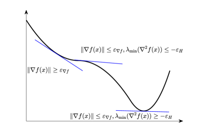
Figure 1: Illustration of three situations in analyzing the convergence to first and second critical point.

3 Sub-sampling for finite-sum minimization

For the finite-sum problem (1), we can estimate $f(x)$, $\nabla f(x)$, and $\nabla^{2}f(x)$ by random sub-sampling, which can drastically reduce the computational complexity. Here, we use $\mathcal{S}_{h}$, $\mathcal{S}_{g}$ and $\mathcal{S}_{B}$ to denote the sample collections for estimating $f(x)$, $\nabla f(x)$ and $\nabla^{2}f(x)$, respectively, where $\mathcal{S}_{h}$, $\mathcal{S}_{g}$ and $\mathcal{S}_{B}\subseteq[n]$. The approximated functions are formed by

$$h(x) =\frac{1}{\left|{{\mathcal{S}_{h}}}\right|}\sum\nolimits_{i\in{\mathcal{S}_{h}}}{{f_{i}}\left(x\right)},$$ (5)

$$g({{x}}) =\frac{1}{{\left|{{\mathcal{S}_{g}}}\right|}}\sum\nolimits_{i\in{\mathcal{S}_{g}}}{\nabla{f_{i}}\left({{x}}\right)},$$ (6)

$$B({{x}}) =\frac{1}{{|{{\mathcal{S}_{B}}}|}}\sum\nolimits_{i\in{\mathcal{S}_{B}}}{{\nabla^{2}}{f_{i}}({{x}})}.$$ (7)

Most papers use operator-Bernstein inequality to probabilistically guarantee such properties, such as [23, 24] use approximate matrix multiplication results as a fundamental primitive in RandNLA [23, 24] to control the approximation error of $\nabla f(x)$. Furthermore, the vector-Bernstein inequality [25, 26] is applied in [8] to obtain the of sub-sample bound of the gradient, which is different from [23]. However, the number of sub-samples depend on the search direction $s$ in advance, which will affect the estimation of sub-sampling. Replacing the condition by (3), we can have

Lemma 2.

Suppose the Assumption 3 holds, if $|{{\mathcal{S}_{g}}}|\geq 16\log({{{2d}}/{\delta}}){{L_{f}^{2}}}/{{\varepsilon_{g}^{2}}}$, then $g(x)$ formed by (6) satisfies $\|\nabla f(x)-g(x)\|\leq{\varepsilon}_{g}$ with probability ($1-\delta$).

Note that, we do not give the proof of above Lemmas as the difference lies on different conditions. We also obtain the approximate gradient $g(x)$ based on above results.

Lemma 3.

Suppose the Assumption 3 holds, If $|\mathcal{S}_{B}|\geq\log({{{2d}}/{\delta}}){{16L_{B}^{2}}}/{{\varepsilon_{B}^{2}}}$, then $B(x)$ formed by (7) satisfies $\|{\nabla^{2}}f(x)-{B(x)}\|\leq{\varepsilon}_{B}$ with probability ($1-\delta$).

In order to reduce the computation cost for updating the $\rho$, we also use the sub-sampling combing with operator-Bernstein inequality to obtain the approximate function probabilistically satisfying (4). Note that, before obtain the approximate function $f(x)$, $s$ has been solved. Thus, we can use $\|s\|$ directly. Furthermore, if the approximate function $h(x)$ satisfies the condition in (4), but could not be guaranteed the bound of $\left\|{\nabla h\left(x\right)-\nabla f\left(x\right)}\right\|$ and $\|{{\nabla^{2}}h(x)-{\nabla^{2}}f(x)}\|$, which will be later used to analyze the radius. Thus, we present a important assumption and use Lemma 1 to derive the upper bound.

Lemma 4.

Suppose the Assumption 3 and 4 hold, If $|{{\cal S}_{h}}|\geq\log(2d/\delta)16\kappa_{f}^{2}/({\varepsilon_{h}^{2}{{\|{{s_{k}}}\|}^{4}}})$, then $h(x)$ formed by (5) satisfies $\|f(x_{k})-h(x_{k})\|\leq{\varepsilon}{{}_{h}}\|s_{k}\|^{2}$ with probability ($1-\delta$). Furthermore, we can also have the upper bounds with the gradient and the Hessian of $h(x)$,

$${\left\|{\nabla h\left(x\right)-\nabla f\left(x\right)}\right\|^{2}}\leq\frac{{\mathbb{I}\left({\left|{{\mathcal{S}_{h}}}\right|<n}\right)}}{{\left|{{\mathcal{S}_{h}}}\right|}}{H_{1}},{\left\|{{\nabla^{2}}h\left(x\right)-{\nabla^{2}}f\left(x\right)}\right\|^{2}}\leq\frac{{\mathbb{I}\left({\left|{{\mathcal{S}_{h}}}\right|<n}\right)}}{{\left|{{\mathcal{S}_{h}}}\right|}}{H_{2}}.$$

4 Stochastic Trust Region method

Algorithm 1 STR with Inexact Hessian and Gradient

1:given $x_{0}$, $r_{2}\geq 1>r_{1}$, $1>\eta>0$, $\varepsilon>0$ and $\Delta_{0},\Delta_{\text{max}}>0$.

2:

3:for $k$=1 to T  do

4:     Compute the approximate gradient $g(x_{k})$ and Hessian matrix $B(x_{k})$ based on (6) and (7).

5:     $\triangleright$ ( if $\|g\left({{x_{k}}}\right)\|\leq{\varepsilon_{\nabla f}}+{\varepsilon_{g}}$, we set $\mathcal{S}_{h}=\mathcal{S}_{g}$)

6:     Compute the direction vector $s_{k}$

$$s_{k}=\text{Subproblem-Solver}(g_{k},B_{k},\Delta_{k}).$$ (8)

7:     Compute the approximate function $h(x_{k})$ and $h(x_{k}+s_{k})$ based on (5).

8:     Compute ${{\tilde{\rho}}_{k}}=\frac{{h\left({{x_{k}}}\right)-h\left({{x_{k}}+{s_{k}}}\right)}}{{{m_{k}}\left(0\right)-{m_{k}}\left({{s_{k}}}\right)}}$

9:     Set $\rho={{{\tilde{\rho}}_{k}}-\frac{{2{\varepsilon_{f}}{\color[rgb]{0,0,0}\|s_{k}\|^{2}}}}{{{m_{k}}\left(0\right)-{m_{k}}\left({{s_{k}}}\right)}}}$

10:     set ${x_{k+1}}=\left\{{\begin{array}[]{*{20}{l}}{{x_{k}}+{s_{k}},}&{\rho\geq\eta,}\\ {{x_{k}},}&{{\rm{otherwise}}{\rm{.}}}\end{array}}\right.$

11:     set ${\Delta_{k+1}}=\left\{{\begin{array}[]{*{20}{l}}{\text{min}\left\{{{\Delta_{\text{max}}},{r_{2}}{\Delta_{k}}}\right\},}&{\rho>\eta,}\\ {{r_{1}}{\Delta_{k}},}&{{\rm{otherwise}}.}\end{array}}\right.$

12:end for

In this section, we consider the stochastic trust region method for solving the constrained optimization problem. At $k$-iteration, the objective function is approximated by a quadratic model within a trust region,

$$\mathop{\min}\nolimits_{s\in\mathbb{R}^{d}}\,{m_{k}}(s),\,\,\,\,\text{subject to}\,\|s\|\leq{\Delta_{k}},$$ (9)

where $\Delta_{k}$ is the radius, and ${m_{k}}(s)$ is defined in (2). The approximated gradient and Hessian are formed based on the conditions in Assumption 2. The conditions of $\varepsilon_{B}$ in (3) does not depend on the search direction $s$, which is the same as in [6, 7]. Moreover, we also define a new parameter $\varepsilon_{g}$, which has the same characteristic as $\varepsilon_{B}$. In addition, the computations of $f(x)$ and $f(x+s)$ are expensive as the objective function is finite-sum structure. Different from [6] and [8], we replace $f(x)$ and $f(x+s)$ with the approximate function $h(x)$ and $h(x+s)$ under the condition (4). This condition is subjected to the search direction $s$. However, the approximate function $h(x)$ and $h(x+s)$ can be derived after obtaining the solution $s$ through Subproblem-Solver. Algorithm 1 presents the process for updating the $x$ and $\Delta$. This section consists of two parts: Firstly, we analyze the role of radius $\Delta$ to ensure that the radius has the lower bound. Secondly, we derive the corresponding iteration complexity under the assumptions we present in Preliminary 2.

4.1 Bounds analysis of radius

First of all, we present three important definition: $\rho_{k}$, $\tilde{\rho}$ and $\rho$. The first two terms are defined as

$${\rho_{k}}=\frac{{f\left({{x_{k}}}\right)-f\left({{x_{k}}+{s_{k}}}\right)}}{{{m_{k}}\left(0\right)-{m_{k}}\left({{s_{k}}}\right)}},{{\tilde{\rho}}_{k}}=\frac{{h\left({{x_{k}}}\right)-h\left({{x_{k}}+{s_{k}}}\right)}}{{{m_{k}}\left(0\right)-{m_{k}}\left({{s_{k}}}\right)}}.$$

Based on the inequality (4) in Assumption 2, we have

$$\left|{{\rho_{k}}-{{\tilde{\rho}}_{k}}}\right|=\left|{\frac{{f\left({{x_{k}}}\right)-h\left({{x_{k}}}\right)-\left({f\left({{x_{k}}+{s_{k}}}\right)-h\left({{x_{k}}+{s_{k}}}\right)}\right)}}{{{m_{k}}\left(0\right)-{m_{k}}\left({{s_{k}}}\right)}}}\right|\leq\frac{{2{\varepsilon_{h}}\|s_{k}\|^{2}}}{{{m_{k}}\left(0\right)-{m_{k}}\left({{s_{k}}}\right)}},$$

that is

$${{\tilde{\rho}}_{k}}-\frac{{2{\varepsilon_{h}}\|s_{k}\|^{2}}}{{{m_{k}}\left(0\right)-{m_{k}}\left({{s_{k}}}\right)}}\leq{\rho_{k}}\leq\frac{{2{\varepsilon_{h}}{\|s_{k}\|^{2}}}}{{{m_{k}}\left(0\right)-{m_{k}}\left({{s_{k}}}\right)}}+{{\tilde{\rho}}_{k}}.$$

Then, define $\rho={{\tilde{\rho}}_{k}}-\frac{{2{\varepsilon_{h}}{\|s_{k}\|^{2}}}}{{{m_{k}}\left(0\right)-{m_{k}}\left({{s_{k}}}\right)}}$. If $\rho\geq{\eta}$, we can obtain ${\rho_{k}}\geq{\eta}$. Thus, in the following analysis, we consider the size of $\rho$ that derive the desired lower bound of the radius.

Before giving the analyses, we briefly present the processing that why the $\Delta$ do not approximate to zero. If ${\rho}>{\eta}$, the current iteration will be successful and the radius $\Delta$ will increase by a factor of $r_{2}$. Thus, we consider that whether there is a constant $C$ such that $\Delta<C$ and the current iteration is successful simultaneously. Then we can see that such constant $C$ is our desired bound of $\Delta$ due to the fact that $\Delta$ will increase again under the successful iteration. What’s more, such constant plays a critical role in determining the iteration complexity.

Instead of computing the $\rho$ directly, we consider another relationship, that is

$$1-\rho=\frac{{{m_{k}}\left(0\right)-{m_{k}}\left({{s_{k}}}\right)-\left({h\left({{x_{k}}}\right)-h\left({{x_{k}}+{s_{k}}}\right)}\right)+2{\varepsilon_{h}}{\|s_{k}\|^{2}}}}{{{m_{k}}\left(0\right)-{m_{k}}\left({{s_{k}}}\right)}}$$ (10)

As long as $1-\rho<1-\eta$, we can see that $\rho>\eta$. Here, we consider the upper and lower bound of denominator and numerator in (10) in Lemma 5 and Lemma 6, respectively. Moreover, we separately give the corresponding bound under the index sets $\mathcal{S}_{\nabla f}$ and $\mathcal{S}_{H}$.

Lemma 5.

Suppose the Assumption 2 and 3 hold, $m_{k}(s)$ is defined in (2). For the case of $x_{k}\in\mathcal{S}_{\nabla f}$, if $m_{k}(s_{k})\leq m_{k}(s_{k}^{C})$, where $s_{k}^{C}$ is the Cauchy point, then we have

$${m_{k}}(0)-{m_{k}}({s_{k}})\geq\frac{1}{2}({\varepsilon_{\nabla f}}-{\varepsilon_{g}})\min\left\{{{\Delta_{k}},({{{\varepsilon_{\nabla f}}-{\varepsilon_{g}}}})/{{{\kappa_{H}}}}}\right\},$$

For the case of $x_{k}\in\mathcal{S}_{H}$, that is ${\lambda_{\text{min}}}({\nabla^{2}f(x_{k})})\leq-{\varepsilon_{H}}$, there exist a vector $s_{k}$ such that $\langle{g({x_{k}}),{s_{k}}}\rangle\leq 0$, ${s_{k}^{T}\nabla^{2}f(x_{k}){s_{k}}}<-v_{0}\Delta_{k}^{2}$, and $\left\|{{s_{k}}}\right\|={\Delta_{k}}$, where $v_{0}\geq\varepsilon_{H}$, then we have

$$m_{k}(0)-{m_{k}}(s_{k})\geq\frac{1}{2}({{\varepsilon_{H}}-{\varepsilon_{B}}})\Delta_{k}^{2}.$$

The solution $S_{k}$ for the Subproblem-Solver is based on subproblem in (2). For the case of $x_{k}\in\mathcal{S}_{\nabla f}$, we use the Cauchy point [3]; while for the case of $x_{k}\in\mathcal{S}_{H}$, there are many methods to derive the solution, such as Shift-and-invert [27], Lanczos [28] and Negative-Curvature [29]. We do not present the details information, which beyond our scope of this paper.

Lemma 6.

Suppose the Assumption 1, 2 and 4 hold, based on the definition of $m_{k}(s)$ in (2), we have

$${m_{k}}\left(0\right)-{m_{k}}\left({{s_{k}}}\right)-\left({h\left({{x_{k}}}\right)-h\left({{x_{k}}+{s_{k}}}\right)}\right)\leq 2\left({\frac{{\mathbb{I}\left({\left|{{\mathcal{S}_{h}}}\right|<n}\right)}}{{\left|{{\mathcal{S}_{h}}}\right|}}H_{1}+{\varepsilon_{g}}}\right){\Delta_{k}}+\frac{3}{2}\left({\frac{{\mathbb{I}\left({\left|{{\mathcal{S}_{h}}}\right|<n}\right)}}{{\left|{{\mathcal{S}_{h}}}\right|}}{H_{2}}+L_{H}{\Delta_{k}}+{\varepsilon_{B}}}\right)\Delta_{k}^{2}.$$

If $\mathcal{S}_{h}=\mathcal{S}_{g}$, we have

$${m_{k}}\left(0\right)-{m_{k}}\left({{s_{k}}}\right)-\left({h\left({{x_{k}}}\right)-h\left({{x_{k}}+{s_{k}}}\right)}\right)\leq\frac{3}{2}\left({\frac{{\mathbb{I}\left({\left|{{\mathcal{S}_{h}}}\right|<n}\right)}}{{\left|{{\mathcal{S}_{h}}}\right|}}{H_{2}}+L_{H}{\Delta_{k}}+{\varepsilon_{B}}}\right)\Delta_{k}^{2}.$$

Note that, in Algorithm 1, for the case of $\|g\left({{x_{k}}}\right)\|\leq{\varepsilon_{\nabla f}}+{\varepsilon_{g}}$, that is

$\left\|{\nabla f\left({{x_{k}}}\right)}\right\|\leq\left\|{g\left({{x_{k}}}\right)}\right\|+\left\|{\nabla f\left({{x_{k}}}\right)-g\left({{x_{k}}}\right)}\right\|\leq{\varepsilon_{\nabla f}}+{\varepsilon_{g}}+{\varepsilon_{g}}={\varepsilon_{\nabla f}}+2{\varepsilon_{g}}$,

we set $\mathcal{S}_{h}=\mathcal{S}_{g}$. $x\in\mathcal{S}_{H}$, in which $\left\|{\nabla f\left({{x_{k}}}\right)}\right\|\leq{\varepsilon_{\nabla f}}$, satisfies such case. Thus, we give the $\Delta_{\text{min2}}$ in (11) based on such implementation, which is key for analyses. The reason we make such implementation is to ensure that there is lower bound of radius. What’s more, the parameters’ setting is more simple. Based on above lemmas, we analyze the minimal radius.

Lemma 7.

In Algorithm 1, suppose the Assumption 1- 4 hold, let $|{{\mathcal{S}_{h}}}|=\min\{n,\max\{H_{1}/\varepsilon_{g},H_{2}/\varepsilon_{B}\}\}$, $1>r_{1}>0$, there will be a non-zero radium

$${\Delta_{\text{min}}}=\min\left\{{{\Delta_{\text{min1}}},{\Delta_{\text{min2}}}}\right\},$$ (11)

where the parameters satisfy

$${\Delta_{\text{min1}}}= {\kappa_{1}}\left({{\varepsilon_{\nabla f}}-{\varepsilon_{g}}}\right),{\kappa_{1}}={r_{1}}\min\left\{{\frac{1}{{{\kappa_{H}}}},\frac{1}{{40}}\left({1-\eta}\right),\sqrt{\frac{1}{{12{L_{H}}}}\left({1-\eta}\right)}}\right\},$$ (12)

$${\Delta_{\text{min2}}}= {\kappa_{2}}\left({{\varepsilon_{H}}-{\varepsilon_{B}}}\right),{\kappa_{2}}={r_{1}}\frac{1}{{6{L_{H}}}}\left({1-\eta}\right),$$ (13)

$${\varepsilon_{g}}= \frac{1}{{16}}\left({1-\eta}\right)\left({{\varepsilon_{\nabla f}}-{\varepsilon_{g}}}\right),$$

$${\varepsilon_{B}}= {\varepsilon_{h}}=\frac{1}{{10}}\left({1-\eta}\right)\left({{\varepsilon_{H}}-{\varepsilon_{B}}}\right).$$

In particular, $\Delta_{\text{min1}}$ belongs to the case of $x\in\mathcal{S}_{\nabla f}$ and $\Delta_{\text{min2}}$ belongs to the case of $x\in\mathcal{S}_{H}$.

4.2 Convergence and iteration complexity

In this section, we present the successful and unsuccessful iteration complexity based on Lemma 7 including $x\in\mathcal{S}_{\nabla f}$ and $k\in\mathcal{S}_{H}$, and then provide the total number of iterations.

Theorem 1.

In Algorithm 1, suppose the Assumption 1- 4 hold, let $|{{\mathcal{S}_{h}}}|=\min\{n,\max\{H_{1}/\varepsilon_{g},H_{2}/\varepsilon_{B}\}\}$, $\{{f({{x_{k}}})}\}$ is bounded below by $f_{\text{low}}$, the number of successful iterations ${T_{\text{suc}}}$ is no large than

$${\kappa_{3}}{\rm{max}}\{{{{({{\varepsilon_{\nabla f}}-{\varepsilon_{g}}})}^{-2}},{{({\varepsilon_{H}}-{\varepsilon_{B}})}^{-3}}}\},$$

where ${\kappa_{3}}=2\left({f\left({{x_{0}}}\right)-{f_{low}}}\right){\rm{max}}\left\{{1/\left({\eta{\kappa_{1}}}\right),1/\left({\eta\kappa_{2}^{2}}\right)}\right\}$, $\kappa_{1}$ and $\kappa_{2}$ are defined in (12) and (13). The number of unsuccessful iterations $T_{\text{unsuc}}$ is at most

$$\frac{1}{{-\log{r_{1}}}}\left({\log\left({\frac{{{\Delta_{{\text{max}}}}}}{{{\Delta_{{\text{min}}}}}}}\right)-T\log{r_{2}}}\right).$$

where ${\Delta_{\text{max}}}$ and ${\Delta_{\text{min}}}$ are defined in (11) and Algorithm 1, $1>{r}_{1}>0$ and $r_{2}\geq 1$. Thus, the total number of iterations is

$$\mathcal{O}\left({\max\{{{{({\varepsilon_{\nabla f}}-{\varepsilon_{g}})}^{-2}},{{({\varepsilon_{H}}-{\varepsilon_{B}})}^{-3}}}\}}\right)$$

After the $|T_{\text{suc}}|+|T_{\text{unsuc}}|$ iterations, it will fall into $\mathcal{S}_{*}$ and converge to the stationary point. As can be seen from above Theorems, we make two conclusions: the first is the order of iteration complexities are the same as [5] and [7] if the parameters $\varepsilon_{g}$ and $\varepsilon_{B}$ are set properly according to $\varepsilon_{\nabla f}$ and $\varepsilon_{H}$ respectively; the second is that when $|{{\mathcal{S}_{h}}}|<n$, the total number of computation iteration including computing the function is less than that of [5] and [7]; when $|{{\mathcal{S}_{h}}}|=n$, our result is equal to[5] and [7]. Thus, our proposed algorithm is more general.

5 Stochastic Adaptive Regularization using Cubics

Algorithm 2 SARC with the Inexact Hessian and Gradient

1:given $x_{0}$, $r_{2}\geq 1>r_{1}$, $1>\eta>0$, $\varepsilon>0$ and $\sigma_{\text{min}}>0$.

2:

3:for $k$=1 to T  do

4:     Compute the approximate gradient $g(x_{k})$ and Hessian matrix $B(x_{k})$ based on (6) and (7).

5:     $\triangleright$ ( if $||g\left({{x_{k}}}\right)||\leq{\varepsilon_{\nabla f}}+{\varepsilon_{g}}$, we set $\mathcal{S}_{h}=\mathcal{S}_{g}$)

6:     Compute the direction vector $s_{k}$

$$s_{k}=\text{Subproblem-Solver}(g(x_{k}),B(x_{k}),\sigma_{k}).$$ (14)

7:     Compute the approximate function $h(x_{k})$ and $h(x_{k}+s_{k})$ based on (5).

8:     Compute ${{\tilde{\rho}}_{k}}=\frac{{h\left({{x_{k}}}\right)-h\left({{x_{k}}+{s_{k}}}\right)}}{{{p_{k}}\left(0\right)-{p_{k}}\left({{s_{k}}}\right)}}$

9:     Set $\rho={{{\tilde{\rho}}_{k}}-\frac{{2{\varepsilon_{f}}/{\color[rgb]{0,0,0}\sigma^{2}_{k}}}}{{{p_{k}}\left(0\right)-{p_{k}}\left({{s_{k}}}\right)}}}$

10:     set ${x_{k+1}}=\left\{{\begin{array}[]{*{20}{l}}{{x_{k}}+{s_{k}},}&{\rho\geq\eta,}\\ {{x_{k}},}&{{\rm{otherwise}}{\rm{.}}}\end{array}}\right.$

11:     set ${\sigma_{k+1}}=\left\{{\begin{array}[]{*{20}{l}}{\max\left\{{{\sigma_{\text{min}}},{r_{1}}{\sigma_{k}}}\right\},}&{\rho>\eta,}\\ {{r_{2}}{\sigma_{k}},}&{{\rm{otherwise}}.}\end{array}}\right.$

12:end for

In this section, we consider the stochastic adaptive regularization using Cubics (SARC) method, which solves the following unconstrained minimization problem at each iteration:

$$\mathop{\min}\nolimits_{s\in\mathbb{R}^{d}}p_{k}(s):=m_{k}(s)+\frac{{{\sigma_{k}}}}{3}{\|s\|^{3}},$$ (15)

where $m_{k}(s)$ is defined in (2), and $\sigma_{k}$ is an adaptive parameter that can be considered as the reciprocal of the trust-region radius. Algorithm 2 presents the process for updating the $x_{k}$ and $\sigma_{k}$. Similar to the analysis as in [4], $\sigma_{k}$ in the cubic term actually performs one more task, besides accounting for the discrepancy between the objective function and its corresponding second-order Taylor expansion, but also for the difference between the exact and approximate function, gradient and Hessian. The update rules of $\sigma$ is analogous to stochastic region method. $\sigma$ will decrease if sufficient decrease is obtained in some measure of relative objective chance, but increase otherwise. Following the framework of STR, we analyze SARC including two parts: To ensure the existence of the maximal bound of $\sigma$ and present the iterative complexity.

5.1 Bounds analysis of the adaptive parameter

Similar to STR, we present the definition of $\rho$ directly,

$$1-\rho= \frac{{{p_{k}}\left(0\right)-{p_{k}}\left({{s_{k}}}\right)-\left({h\left({{x_{k}}}\right)-h\left({{x_{k}}+{s_{k}}}\right)}\right)+2{\varepsilon_{h}}\|s_{k}\|^{2}}}{{{p_{k}}\left(0\right)-{p_{k}}\left({{s_{k}}}\right)}}$$ (16)

In order to satisfy inequality (16), we need to obtain the lower bound of the numerator in (16). Firstly, we derived the lower bound from the view of a Cauchy pint, but subject to ${p_{k}}\left({{s_{k}}}\right)\leq{p_{k}}\left({s_{k}^{C}}\right)$. Note that the lower bound is almost the same as in [4] and [6], but give the proof from the geometrical explanation.

Lemma 8.

Suppose that the step size $s_{k}$ satisfying ${p_{k}}\left({{s_{k}}}\right)\leq{p_{k}}\left({s_{k}^{C}}\right)$, where $s_{k}^{C}$ is a Cauchy point, defined as

$$s_{k}^{C}= -{\alpha_{k}}g\left({{x_{k}}}\right),{\alpha_{k}}=\mathop{\arg\min}\nolimits_{\alpha\in{\mathbb{R}_{+}}}\left\{{{p_{k}}\left(x_{k}{-\alpha g\left({{x_{k}}}\right)}\right)}\right\},$$

for all $k\geq 0$, we have that

$p_{k}(0)-{p_{k}}(s_{k})\geq\frac{1}{10}\left\|{{g_{k}}}\right\|\min\left\{{{\left\|{{g_{k}}}\right\|}/{{\left\|{{B_{k}}}\right\|}},\sqrt{{{\left\|{{g_{k}}}\right\|}}/(\sigma_{k})}}\right\}.$

Specifically, we set ${\alpha}=2/(\|B_{k}\|+\sqrt{{\|B_{k}\|}^{2}+4{\sigma_{k}}\|g_{k}\|})$ and $s_{k}=-\alpha g(x_{k})$ that satisfy above inequality. Furthermore, we can also obtain the upper bound of the step $\|s_{k}\|$, $k>0$, satisfies $\|s_{k}\|\leq{{11}}/{4}\max\{{{{\|{B({x_{k}})}\|}}/{{{\sigma_{k}}}},\sqrt{{{\|{g({x_{k}})}\|}}/{{{\sigma_{k}}}}}}\}.$

Following the subspace analysis in the cubic model as in [4] and [5], in order to widen the scope of convergence analysis and iteration complexity, we also consider the step size $s_{k}$ on the following conditions

$$\left\langle{g\left({{x_{k}}}\right),{s_{k}}}\right\rangle+s_{k}^{T}{B_{k}}{s_{k}}+{\sigma_{k}}{\left\|{{s_{k}}}\right\|^{3}}=0,$$ (17)

$$s_{k}^{T}{B_{k}}{s_{k}}+{\sigma_{k}}{\left\|{{s_{k}}}\right\|^{3}}\geq 0,$$ (18)

$$\left\|{\nabla{p_{k}}\left({{s_{k}}}\right)}\right\|\leq{\theta_{k}}\left\|{\nabla g\left({{x_{k}}}\right)}\right\|,{\theta_{k}}\leq{\kappa_{\theta}}\text{min}\left\{{1,\left\|{{s_{k}}}\right\|}\right\},{\kappa_{\theta}}<1.$$ (19)

Thus, we can also obtain lower bound of the numerator in (16), which will be used for analyzing the convergence and iteration complexity in the case of the saddle point.

Lemma 9.

Given the conditions of $s_{k}$ in (17) and (18), we have

$$p(0)-{p_{k}}(s_{k})\geq\frac{{{\sigma_{k}}}}{6}{\|{{s_{k}}}\|^{3}}.$$

Furthermore, suppose Assumption 1 and 2, and the condition (19) hold, for $\left\|{g\left({{x_{k+1}}}\right)}\right\|\geq{\varepsilon_{\nabla f}}-{\varepsilon_{g}}$, we have

$$\left\|{g\left({{x_{k+1}}}\right)}\right\|\leq{\kappa_{s}}{\left\|{{s_{k}}}\right\|^{2}},$$ (20)

where

$$\begin{array}[]{l}{\kappa_{s}}=\min\left\{{\frac{{2{\varepsilon_{B}}+\left({{L_{H}}+{\sigma_{k}}}\right)+2{\kappa_{\theta}}{\varepsilon_{g}}+{\kappa_{\theta}}{L_{\nabla f}}}}{{\left({1-{\theta_{k}}}\right)}},\frac{{{L_{H}}+{\sigma_{k}}+{\kappa_{\theta}}{L_{\nabla f}}}}{{1-{\theta_{k}}-{\zeta_{1}}-{\zeta_{2}}}}}\right\},{\zeta_{1}},{\zeta_{2}}<1\\ {\varepsilon_{B}}\leq{\zeta_{1}}\left({{\varepsilon_{\nabla f}}-{\varepsilon_{g}}}\right),{\varepsilon_{g}}\leq{\zeta_{2}}\left({{\varepsilon_{\nabla f}}-{\varepsilon_{g}}}\right)\end{array}$$

Different from the STR, we can also derive the relationship between $g(x_{k+1})$ and $\|s_{k}\|$. The core process of the proof is based on cubic regularization of Newton method [30]. Such a relationship leads to the improved iteration complexity. Besides lower bound of the numerator in (16), we can also obtain the corresponding upper bound of the denominator, which is similar to Lemma 6. Thus, we do not provide the proof.

Lemma 10.

Suppose the Assumption 1, 2 and 4 hold, at $k$-iteration, we have

$${p_{k}}\left(0\right)-{p_{k}}\left({{s_{k}}}\right)-\left({h\left({{x_{k}}}\right)-h\left({{x_{k}}+{s_{k}}}\right)}\right)$$

$$\leq 2\left({\frac{\mathbb{I}{\left({\left|{{{\cal S}_{h}}}\right|<n}\right)}}{{\left|{{{\cal S}_{h}}}\right|}}{H_{1}}+{\varepsilon_{g}}}\right)\left\|{{s_{k}}}\right\|+\frac{3}{2}\left({\frac{\mathbb{I}{\left({\left|{{{\cal S}_{h}}}\right|<n}\right)}}{{\left|{{{\cal S}_{h}}}\right|}}{H_{2}}+{\varepsilon_{B}}}\right){\left\|{{s_{k}}}\right\|^{2}}+\left({\frac{3}{2}{L_{H}}-\frac{1}{3}{\sigma_{k}}}\right){\left\|{{s_{k}}}\right\|^{3}}$$

If $\mathcal{S}_{h}=\mathcal{S}_{g}$, we have

$${p_{k}}\left(0\right)-{p_{k}}\left({{s_{k}}}\right)-\left({h\left({{x_{k}}}\right)-h\left({{x_{k}}+{s_{k}}}\right)}\right)\leq\frac{3}{2}\left({\frac{\mathbb{I}{\left({\left|{{{\cal S}_{h}}}\right|<n}\right)}}{{\left|{{{\cal S}_{h}}}\right|}}{H_{2}}+{\varepsilon_{B}}}\right){\left\|{{s_{k}}}\right\|^{2}}+\left({\frac{3}{2}{L_{H}}-\frac{1}{3}{\sigma_{k}}}\right){\left\|{{s_{k}}}\right\|^{3}}.$$

Based on the above lemmas, we can derive the upper bound of adaptive parameter $\sigma$, which is used to analyze the iteration complexity. Furthermore, the parameters’ setting, such as $\varepsilon_{g}$, $\varepsilon_{B}$ and $\varepsilon_{h}$ are similar to that of Lemma 7.

Lemma 11.

In Algorithm 2, suppose Assumption 1-4 hold, let $|{{\mathcal{S}_{h}}}|=\min\{n,\max\{H_{1}/\varepsilon_{g},H_{2}/\varepsilon_{B}\}\}$, $r_{2}>1$, the parameter $\sigma$ is bounded by

$${\sigma_{\text{max}}}=\max\left\{{{\sigma_{\text{max1}}},{\sigma_{\text{max2}}}}\right\},$$ (21)

where

$${\sigma_{{\text{max1}}}}= {\kappa_{4}}\frac{1}{{({\varepsilon_{\nabla f}}-{\varepsilon_{g}})}},{\sigma_{\text{max2}}}=\frac{9}{2}{r_{2}}{L_{H}},$$

$${\kappa_{4}}= {r_{2}}\left\{{\kappa_{H}^{2},\frac{{{{\left({304\left({3{\varepsilon_{B}}+2{\varepsilon_{h}}}\right)}\right)}^{2}}}}{{\left({1-\eta}\right)}},\frac{9}{2}({\varepsilon_{\nabla f}}-{\varepsilon_{g}}){L_{H}}}\right\},$$ (22)

$${\varepsilon_{g}}= \frac{1}{{220}}\left({1-\eta}\right)({\varepsilon_{\nabla f}}-{\varepsilon_{g}}),$$

$${\varepsilon_{B}}= {\varepsilon_{h}}=\frac{1}{{36}}\left({1-\eta}\right)\left({{\varepsilon_{H}}-{\varepsilon_{B}}}\right).$$

In particular, $\sigma_{\text{min1}}$ belongs to the case of $x\in\mathcal{S}_{\nabla f}$ and $\sigma_{\text{min2}}$ belongs to the case of $x\in\mathcal{S}_{H}$.

5.2 Analysis of convergence and iteration complexity

Based on above lemmas, we present the iteration complexity. Different from STR, we derive two kinds of complexity. The first one has the same order as STR while the second is better or equal to STR. The difference lies that if the criterion conditions in (19) is satisfied, the iteration complexity to the stationary point is improved.

Theorem 2.

In Algorithm 2, suppose the Assumption 1- 4 hold, let $|{{\mathcal{S}_{h}}}|=\min\{n,\max\{H_{1}/\varepsilon_{g},H_{2}/\varepsilon_{B}\}\}$, $\{{f({{x_{k}}})}\}$ is bounded below by $f_{\text{low}}$, the number of successful iterations ${T_{\text{suc}}}$ is no large than

$${\kappa_{5}}\max\{{{{({\varepsilon_{\nabla f}}-{\varepsilon_{g}})}^{-2}},{{({{\varepsilon_{H}}-{\varepsilon_{B}}})}^{-3}}}\},$$

where ${\kappa_{5}}=({f({{x_{0}}})-{f_{{\rm{low}}}}})\max\{{5/(\eta\kappa_{4}^{-1/2}),6{\sigma_{{\rm{max2}}}}/\eta}\}$, $\kappa_{4}$ is defined in (22). If the conditions (17)-(19) are satisfied, then the number of successful iterations $T_{\text{unsuc}}$ is at most

$${\kappa_{6}}\max\{{{{({\varepsilon_{\nabla f}}-{\varepsilon_{g}})}^{-3/2}},{{({{\varepsilon_{H}}-{\varepsilon_{B}}})}^{-3}}}\},$$

where ${\kappa_{6}}=({f({{x_{0}}})-{f_{{\text{low}}}}})\max\{{6\kappa_{s}^{3/2}/({\eta{\sigma_{{\text{min}}}}}),6{\sigma_{{\text{max2}}}}/\eta}\}$, $\kappa_{s}$ is defined (20).

As can be seen above results, our proposed method has the same order of iteration complexity as in [6] and [7]. However, our algorithm does not require the full computation of function and gradient with the finite-sum structure such that reduce the computation cost properly.

6 Experiment

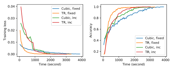
Figure 2: Training loss/accuracy vs running time for different schemes of second-order methods. Note that TR-full and ARC-full only finish 1 epoch after 3000 seconds, so we omit them in the plot.

In this section, we give a comprehensive comparison among trust region and ARC algorithms. Our goal is not to show TR/ARC methods are state-of-the-art compared with other solvers; we are trying to present different variances of TR and ARC, and show using a fixed batch size to estimate both gradient and Hessian is the best choice for large-scale optimization. We compare following variants:

• Stochastic TR with fixed batch size (TR, fixed): Both Hessian and gradient are estimated through a fixed batch size at each iteration. In our experiment, we choose batch size $|B_{g}|=|B_{H}|=256$.

• Stochastic TR with growing batch size (TR, inc): As above, both Hessian and gradient are estimated through a batch of samples, except that the sample size is increasing with epochs: At the early stage we feed a crude estimation of $\nabla f(x)$ and $\nabla^{2}f(x)$ on small batch, then gradually increase the batch size to give better gradient and Hessian information. In practice we multiply the batch size by a factor of $2$ for every $10$ epochs until memory is used up.

• Stochastic TR with exact gradient and subsampled Hessian (TR, full): We use implementation similar with [6, 7]. At each iteration the gradient is exact, while the Hessian is approximated on a batch of $256$ samples.

• Stochastic ARC with fixed batch size (Cubic, fixed): This is similar to stochastic TR, the batch size is fixed to $|B_{g}|=|B_{H}|=256$.

• Stochastic ARC with growing batch size (Cubic, inc): Similar to stochastic TR with increasing batch size, we double the batch size once every $10$ epochs to estimate both Hessian and gradient.

• ARC with exact gradient and subsampled Hessian (Cubic, full): The gradient is exactly computed while the Hessian is approximated on a batch of $256$ samples.

Note that the ARC-inc algorithm is proposed in [8]; TR-inc is a generalization of that to the trust region case; TR-full and ARC-full are proposed in [6]; TR-fixed and ARC-fixed are our method analyzed in this paper.

We train a VGG16 network on CIFAR10 dataset using the above algorithms and evaluate the performance according to training loss and test accuracy with respect to training time. All the experiments are run on a machine with 1 Titan Xp GPU. The result is reported in Figure 2.

Note that TR-full and ARC-full take 3500 seconds while TR-fixed and ARC-fixed only take 40 seconds for each epoch. Thus we omit the full gradient versions on the plot since there will be only one point there. This shows that calculating the full gradient for each update is too expensive for solving large-scale problems like deep learning. Apart from that we notice both Cubic and TR on fixed batch size are faster than their growing batch size version, this validates our guess that sampling a fixed number of data to estimate gradient and Hessian is sufficient to make trust region and ARC work, and this scheme turns out to be more efficient than sample a growing batch over time. Moreover, in our task, the trust region algorithm is faster than ARC algorithm. However, we are not sure whether this phenomenon also applies to other tasks.

7 Conclusion

In this paper, we present a family of stochastic trust region method and stochastic cubic regularization method under inexact gradient and Hessian matrix. Furthermore, in order to reduce the computation cost for the function value of $f(x)$ in evaluating the role of $\rho$, we also present a sub-sample technique to estimate the function. We provide the theoretical analysis of convergence and iteration complexity and obtain that we keep the same order of iteration complexity but reduce the computation cost per iteration. We apply our proposed method to deep learning application which outperforms the previous second-order methods.

Appendix A Proof of Sub-sampling

Proof of Lemma 1

Proof.

Based on the $\sum\nolimits_{i=1}^{m}{{v_{i}}}=\vec{0}$, and permutation and combination, For the case that $\cal A$ is a non-empty, uniformly random subset of $[m]$, we have

$${\mathbb{E}_{\cal A}}{{{\left\|{\sum\nolimits_{b\in\mathcal{A}}{{v_{b}}}}\right\|}^{2}}}= {\mathbb{E}_{\cal A}}\left[{\sum\nolimits_{b\in{\cal A}}{{{\left\|{{v_{b}}}\right\|}^{2}}}}\right]+\frac{1}{{C_{n}^{A}}}\sum\limits_{i\in[n]}{\left\langle{{v_{i}},\frac{{C_{n-1}^{A-1}\left({A-1}\right)}}{{n-1}}\sum\limits_{i\neq j}{{v_{j}}}}\right\rangle}$$

$$= A\frac{1}{n}\sum\nolimits_{i=1}^{n}{v_{i}^{2}}+\frac{{A\left({A-1}\right)}}{{n\left({n-1}\right)}}\sum\nolimits_{i\in[n]}{\left\langle{{v_{i}},\sum\nolimits_{i\neq j}{{v_{j}}}}\right\rangle}$$

$$= A\frac{1}{n}\sum\nolimits_{i=1}^{n}{v_{i}^{2}}+\frac{{A\left({A-1}\right)}}{{n\left({n-1}\right)}}\sum\nolimits_{i\in[n]}{\left\langle{{v_{i}},-{v_{i}}}\right\rangle}$$

$$= \frac{{A\left({n-A}\right)}}{{\left({n-1}\right)}}\frac{1}{n}\sum\nolimits_{i=1}^{n}{v_{i}^{2}}\leq A\mathbb{I}\left({A<n}\right)\frac{1}{n}\sum\nolimits_{i=1}^{n}{v_{i}^{2}}.$$

Thus, we have ${\mathbb{E}_{\cal A}}{{{\left\|\frac{1}{A}{\sum\nolimits_{b\in\mathcal{A}}{{v_{b}}}}\right\|}^{2}}}=\frac{1}{A^{2}}{\mathbb{E}_{\cal A}}{{{\left\|{\sum\nolimits_{b\in\mathcal{A}}{{v_{b}}}}\right\|}^{2}}}\leq\frac{{\mathbb{I}\left({A<n}\right)}}{A}\frac{1}{n}\sum\limits_{i=1}^{n}{v_{i}^{2}}.$ ∎

Proof of Lemma 4

Proof.

Let us define ${X_{i}}={f_{i}}(x)-f(x),i\in{\mathcal{S}_{h}}.$ Based on the Assumption 3, we have

$$|{{X_{i}}}|=|{{f_{i}}(x)-f(x)}|\leq|{{f_{i}}(x)}|+|{f(x)}|\leq 2{\kappa_{f}}\Rightarrow{|{{X_{i}}}|^{2}}\leq 4\kappa_{f}^{2},$$

which satisfying the conditions $\mathbb{E}[{|{{X_{i}}}|}]=0,\mathbb{E}[{X_{i}^{2}}]\leq 4\kappa_{f}^{2}.$ Define the new variable

$${Z_{1}}= {f_{s}}(x)-f\left(x\right)=\frac{1}{{\left|{{\mathcal{S}_{h}}}\right|}}\sum\nolimits_{j\in\left|{{\mathcal{S}_{h}}}\right|}{\left({{f_{i}}\left(x\right)-f\left(x\right)}\right)},$$

$${Z_{2}}= \sum\nolimits_{j\in\left|{{\mathcal{S}_{h}}}\right|}{\left({{f_{i}}\left(x\right)-f\left(x\right)}\right)}.$$

Based on the Operator-Bernstein inequality [31], We give probability about the condition in Assumption 2, we have $|{{Z_{2}}}|=\left|{{\mathcal{S}_{h}}}\right|\left|{{Z_{1}}}\right|\geq\left|{{\mathcal{S}_{h}}}\right|{\varepsilon_{h}}{\|s_{k}\|^{2}}$, then $\Pr\left[{\left|{{Z_{2}}}\right|>\left|{{\mathcal{S}_{h}}}\right|{\varepsilon_{h}}{\Delta^{2}_{{k}}}}\right]\leq 2d\exp\left({-\frac{{{{\left({\left|{{\mathcal{S}_{h}}}\right|{\varepsilon_{h}}{\|s_{k}\|^{2}}}\right)}^{2}}}}{{4\left|{{\mathcal{S}_{h}}}\right|4\kappa_{f}^{2}}}}\right)\leq\delta.$ Thus, the cardinality of $\mathcal{S}_{h}$ should satisfy $\left|{{\mathcal{S}_{h}}}\right|\geq\frac{{16\kappa_{f}^{2}}}{{\varepsilon_{h}^{2}\|s_{k}\|^{4}}}\log\left({\frac{2d}{\delta}}\right),$

Furthermore, based on Lemma 1 and Assumption 4, we can also have the upper bounds with respect to the gradient and the Hessian of $h(x)$,

$${\left\|{\nabla h\left(x\right)-\nabla f\left(x\right)}\right\|^{2}}\leq\frac{{\mathbb{I}\left({\left|{{\mathcal{S}_{h}}}\right|<n}\right)}}{{\left|{{\mathcal{S}_{h}}}\right|}}{H_{1}},{\left\|{{\nabla^{2}}h\left(x\right)-{\nabla^{2}}f\left(x\right)}\right\|^{2}}\leq\frac{{\mathbb{I}\left({\left|{{\mathcal{S}_{h}}}\right|<n}\right)}}{{\left|{{\mathcal{S}_{h}}}\right|}}{H_{2}}.$$

∎

Appendix B Proof for Stochastic Trust Region

Proof of Lemma 5

Proof.

For the case $x_{k}\in\mathcal{S}_{\nabla f}$, through adding and subtracting the term $\nabla f(x_{k})$, we have the lower bound of $\|g(x)\|$,

$$\|{g(x_{k})}\| =\|{g(x_{k})-\nabla f(x_{k})+\nabla f(x_{k})}\|$$

$$\geq\|{\nabla f(x_{k})}\|-\|{g(x_{k})-\nabla f(x_{k})}\|$$

$$\geq{\varepsilon_{\nabla f}}-{\varepsilon_{g}},$$

where the last inequality is based on the approximation of $\nabla f(x_{k})$ in Assumption 2. Following the lower bound on the decrease of the proximal quadratic function ${m_{k}}({{s}})$ from (4.20) in [32], we have

$$m_{k}(0)-{m_{k}}(s_{k}) \geq\frac{1}{2}\|{g({{x_{k}}})}\|\min\left\{{{\Delta_{k}},\frac{{\|{g({{x_{k}}})}\|}}{{\|{B({{x_{k}}})}\|}}}\right\}\geq\frac{1}{2}({{\varepsilon_{\nabla f}}-{\varepsilon_{g}})}\min\left\{{{\Delta_{k}},\frac{{{\varepsilon_{\nabla f}}-{\varepsilon_{g}}}}{{{\kappa_{H}}}}}\right\},$$

where the last inequality is from above inequality and the bound of ${\left\|{B({x_{k}})}\right\|}$ in Assumption 3.

For the case $x_{k}\in\mathcal{S}_{H}$, through adding and subtracting the term $\nabla^{2}f(x_{k})$, we have

$$\frac{{s_{k}^{T}B({x_{k}}){s_{k}}}}{{\left\|{{s_{k}}}\right\|}}= \frac{{s_{k}^{T}(B({x_{k}})-\nabla^{2}f(x_{k})+\nabla^{2}f(x_{k})){s_{k}}}}{{\left\|{{s_{k}}}\right\|}}$$

$$= \frac{{s_{k}^{T}(B({x_{k}})-\nabla^{2}f(x_{k})){s_{k}}}}{{\left\|{{s_{k}}}\right\|}}+\frac{{s_{k}^{T}\nabla^{2}f(x_{k}){s_{k}}}}{{\left\|{{s_{k}}}\right\|}}$$

$$\leq \left\|{B({x_{k}})-\nabla^{2}f(x_{k})}\right\|+\frac{{s_{k}^{T}\nabla^{2}f(x_{k}){s_{k}}}}{{\left\|{{s_{k}}}\right\|}}$$

$$\leq {\varepsilon_{B}}-{v_{0}}$$

$$\leq {\varepsilon_{B}}-{\varepsilon_{H}}=-\left({{\varepsilon_{H}}-{\varepsilon_{B}}}\right),$$ (23)

where the second inequality is based on the Assumption in 2 and Rayleigh quotient [3]. Using the definition of $m_{k}(s)$ in (2), we have

$$m_{k}(0)-{m_{k}}({{s_{k}}}) =-\left\langle{g({x_{k}}),{s_{k}}}\right\rangle-\frac{1}{2}s_{k}^{T}B\left({{x_{k}}}\right){s_{k}}$$

$$\mathop{\geq}\limits^{{\scriptsize\tiny{1}⃝}}-\frac{1}{2}s_{k}^{T}B\left({{x_{k}}}\right){s_{k}}$$

$$\mathop{\geq}\limits^{{\scriptsize\tiny{2}⃝}}\frac{1}{2}\left({{\varepsilon_{H}}-{\varepsilon_{B}}}\right){\left\|{{s_{k}}}\right\|^{2}}\mathop{=}\limits^{{\scriptsize\tiny{3}⃝}}\frac{1}{2}\left({{\varepsilon_{H}}-{\varepsilon_{B}}}\right)\Delta_{k}^{2},$$

where inequality $\scriptsize\tiny{1}⃝$ is based on $\langle{g({x_{k}}),{s_{k}}}\rangle\leq 0$, inequality $\scriptsize\tiny{2}⃝$ follows from (23), inequality $\scriptsize\tiny{3}⃝$ is based on $\left\|{{s_{k}}}\right\|={\Delta_{k}}$. ∎

Proof of Lemma 6

Proof.

Consider the Taylor expansion for $h(x_{k}+s_{k})$ at $x_{k}$,

$$h\left({{x_{k}}+{s_{k}}}\right)=h\left({{x_{k}}}\right)+\left\langle{{s_{k}},\nabla h\left({{x_{k}}}\right)}\right\rangle+\frac{1}{2}s_{k}^{T}\nabla^{2}h\left({{\xi_{k}}}\right){s_{k}},$$

where ${\xi_{k}}\in\left[{{x_{k}},{x_{k}}+{s_{k}}}\right]$. Based on the definition of $m_{k}(s)$ in (2) and the Taylor expansion of the function $h(x_{k}+s_{k})$ at $x_{k}$ above, we have

$${m_{k}}\left(0\right)-{m_{k}}\left({{s_{k}}}\right)-\left({h\left({{x_{k}}}\right)-h\left({{x_{k}}+{s_{k}}}\right)}\right)$$

$$= -\langle g({x_{k}}),{s_{k}}\rangle-\frac{1}{2}s_{k}^{T}B({x_{k}}){s_{k}}+\left({\left\langle{\nabla h\left({{x_{k}}}\right),{s_{k}}}\right\rangle+\frac{1}{2}s_{k}^{T}{\nabla^{2}}h\left({{\xi_{k}}}\right){s_{k}}}\right)$$

$$= \left\langle{\nabla h\left({{x_{k}}}\right)-g({x_{k}}),{s_{k}}}\right\rangle+\frac{1}{2}s_{k}^{T}\left({{\nabla^{2}}h\left({{\xi_{k}}}\right)-B({x_{k}})}\right){s_{k}}$$ (24)

$$= \left\langle{\nabla h\left({{x_{k}}}\right)-\nabla f\left({{x_{k}}}\right)+\nabla f\left({{x_{k}}}\right)-g({x_{k}}),{s_{k}}}\right\rangle$$

$$+\frac{1}{2}s_{k}^{T}\left({{\nabla^{2}}h\left({{\xi_{k}}}\right)-{\nabla^{2}}f\left({{\xi_{k}}}\right)+{\nabla^{2}}f\left({{\xi_{k}}}\right)-{\nabla^{2}}f\left({{x_{k}}}\right)+{\nabla^{2}}f\left({{x_{k}}}\right)-B({x_{k}})}\right){s_{k}}$$

$$\mathop{\leq}\limits^{{\scriptsize\tiny{1}⃝}} 2\left({\left\|{\nabla h\left({{x_{k}}}\right)-\nabla f\left({{x_{k}}}\right)}\right\|+\left\|{\nabla f\left({{x_{k}}}\right)-g({x_{k}})}\right\|}\right)\left\|{{s_{k}}}\right\|$$

$$+\frac{3}{2}\left({\left\|{{\nabla^{2}}h\left({{\xi_{k}}}\right)-{\nabla^{2}}f\left({{\xi_{k}}}\right)}\right\|+{\left\|{{\nabla^{2}}f\left({{\xi_{k}}}\right)-{\nabla^{2}}f\left({{x_{k}}}\right)}\right\|}+\left\|{{\nabla^{2}}f\left({{x_{k}}}\right)-B({x_{k}})}\right\|}\right){\left\|{{s_{k}}}\right\|^{2}}$$

$$\mathop{\leq}\limits^{{\scriptsize\tiny{2}⃝}} 2\left({\frac{{\mathbb{I}\left({\left|{{\mathcal{S}_{h}}}\right|<n}\right)}}{{\left|{{\mathcal{S}_{h}}}\right|}}H_{1}+{\varepsilon_{g}}}\right)\left\|{{s_{k}}}\right\|+\frac{3}{2}\left({\frac{{\mathbb{I}\left({\left|{{\mathcal{S}_{h}}}\right|<n}\right)}}{{\left|{{\mathcal{S}_{h}}}\right|}}{H_{2}}+L_{H}\left\|{{s_{k}}}\right\|+{\varepsilon_{B}}}\right){\left\|{{s_{k}}}\right\|^{2}}$$

$$\mathop{\leq}\limits^{{\scriptsize\tiny{3}⃝}} 2\left({\frac{{\mathbb{I}\left({\left|{{\mathcal{S}_{h}}}\right|<n}\right)}}{{\left|{{\mathcal{S}_{h}}}\right|}}H_{1}+{\varepsilon_{g}}}\right){\Delta_{k}}+\frac{3}{2}\left({\frac{{\mathbb{I}\left({\left|{{\mathcal{S}_{h}}}\right|<n}\right)}}{{\left|{{\mathcal{S}_{h}}}\right|}}{H_{2}}+L_{H}{\Delta_{k}}+{\varepsilon_{B}}}\right)\Delta_{k}^{2},$$

where inequality $\scriptsize\tiny{1}⃝$ follows from the Holder’s inequality, inequality $\scriptsize\tiny{2}⃝$ is based on the approximation of $\nabla f(x)$ and $\nabla^{2}f(x)$ in Assumption 2, and the Lipschitz continuous of Hessian matrix of $f(x)$ in Assumption 1, inequality $\scriptsize\tiny{3}⃝$ follows from the constraint condition as in the objective (9).

Furthermore, for the case of $\mathcal{S}_{h}=\mathcal{S}_{g}$, the first term of (24) is equal to zero, then we have

$${m_{k}}\left(0\right)-{m_{k}}\left({{s_{k}}}\right)-\left({h\left({{x_{k}}}\right)-h\left({{x_{k}}+{s_{k}}}\right)}\right)\leq\frac{3}{2}\left({\frac{{\mathbb{I}\left({\left|{{\mathcal{S}_{h}}}\right|<n}\right)}}{{\left|{{\mathcal{S}_{h}}}\right|}}{H_{2}}+{\Delta_{k}}+{\varepsilon_{B}}}\right)\Delta_{k}^{2}.$$

∎

Proof of Lemma 7

Proof.

By setting $\frac{{\mathbb{I}\left({\left|{{\mathcal{S}_{h}}}\right|<n}\right)}}{{\left|{{\mathcal{S}_{h}}}\right|}}{H_{1}}\leq{\varepsilon_{g}}$, and $\frac{{\mathbb{I}\left({\left|{{\mathcal{S}_{h}}}\right|<n}\right)}}{{\left|{{\mathcal{S}_{h}}}\right|}}{H_{2}}\leq{\varepsilon_{B}}$, we consider two cases:

For the case $\nabla f(x)>\varepsilon_{\nabla f(x)}$, we assume that ${\Delta_{k}}\leq\frac{{{\varepsilon_{\nabla f}}-{\varepsilon_{g}}}}{{{\kappa_{H}}}}$, which is used for Lemma 5. Combine with (10) and the results in Lemma 5, Lemma 6, and $\|s_{k}\|^{2}<\Delta_{k}^{2}$, we have

$$1-\rho\leq \frac{{2\left({\frac{{\mathbb{I}\left({\left|{{S_{h}}}\right|<n}\right)}}{{\left|{{S_{h}}}\right|}}{H_{1}}+{\varepsilon_{g}}}\right){\Delta_{k}}+\frac{3}{2}\left({\frac{{\mathbb{I}\left({\left|{{S_{h}}}\right|<n}\right)}}{{\left|{{S_{h}}}\right|}}{H_{2}}+L_{H}{\Delta_{k}}+{\varepsilon_{B}}}\right)\Delta_{k}^{2}+2{\varepsilon_{h}}{\Delta^{2}_{k}}}}{{\frac{1}{2}\left({{\varepsilon_{\nabla f}}-{\varepsilon_{g}}}\right){\Delta_{k}}}}$$

$$= \frac{{4{\varepsilon_{g}}+\frac{3}{2}\left({{L_{H}}{\Delta_{k}}+2{\varepsilon_{B}}+\frac{4}{3}{\varepsilon_{h}}}\right){\Delta_{k}}}}{{\frac{1}{2}\left({{\varepsilon_{\nabla f}}-{\varepsilon_{g}}}\right)}}.$$ (25)

In order to have the lower bound radius $\Delta_{k}$ such that $1-\rho\leq 1-\eta$, we consider the parameters’ setting:

• For the first term $4{\varepsilon_{g}}=\frac{1}{4}\left({1-\eta}\right)\left({{\varepsilon_{\nabla f}}-{\varepsilon_{g}}}\right)$, then we define, ${\varepsilon_{g}}=\frac{1}{{16}}\left({1-\eta}\right)\left({{\varepsilon_{\nabla f}}-{\varepsilon_{g}}}\right)$.

• For the second term $\frac{3}{2}\left({L_{H}{\Delta_{k}}+2{\varepsilon_{B}}+{\varepsilon_{h}}}\right){\Delta_{k}}\leq\frac{1}{4}\left({1-\eta}\right)\left({{\varepsilon_{\nabla f}}-{\varepsilon_{g}}}\right)$, as $\varepsilon_{B}<1,\varepsilon_{h}<1,\varepsilon_{\nabla f}-\varepsilon_{g}<1$, Thus, as long as

  $${\Delta_{k}}\leq\left({{\varepsilon_{\nabla f}}-{\varepsilon_{g}}}\right)\min\left\{{\frac{1}{{40}}\left({1-\eta}\right),\sqrt{\frac{1}{{12{L_{H}}}}\left({1-\eta}\right)}}\right\}$$ (26)

  we can obtain that $1-\rho\leq 1-\eta$.

At the $k$-iteration, when the radius $\Delta_{k}$ satisfy above condition, the update is successful iteration, as in Algorithm 1, the radius $\Delta_{k}$ will increase by a factor $r_{2}$.

For the case ${\lambda_{\text{min}}}({\nabla^{2}f(x_{k})})\leq-{\varepsilon_{H}}$, based on the results in Lemma 5 and Lemma 6, we have

$$1-\rho\leq\frac{{\frac{3}{2}\left({{L_{H}}{\Delta_{k}}+2{\varepsilon_{B}}+\frac{4}{3}{\varepsilon_{h}}}\right){\Delta_{k}}}}{{\frac{1}{2}\left({{\varepsilon_{H}}-{\varepsilon_{B}}}\right){\Delta_{k}}}}.$$

In order to have the lower bound radius $\Delta_{k}$ such that $1-\rho\leq 1-\eta$, we consider the parameters’ setting:

$${\varepsilon_{B}}={\varepsilon_{h}}=\frac{1}{{20}}\left({1-\eta}\right)\left({{\varepsilon_{H}}-{\varepsilon_{B}}}\right),{\Delta_{k}}\leq\frac{1}{{6{L_{H}}}}\left({1-\eta}\right)\left({{\varepsilon_{H}}-{\varepsilon_{B}}}\right).$$ (27)

Based on above analysis and combine the assumption bound of $\Delta$ at beginning, there exist a minimal radius

$${\Delta_{{\rm{min}}}}=\min\left\{{{\varepsilon_{\nabla f}}-{\varepsilon_{g}},{\varepsilon_{H}}-{\varepsilon_{B}}}\right\}{\kappa_{1}},{\kappa_{1}}={r_{1}}\min\left\{{\frac{1}{{{\kappa_{H}}}},\frac{1}{{40}}\left({1-\eta}\right),\sqrt{\frac{1}{{12{L_{H}}}}\left({1-\eta}\right)},\frac{1}{{10{L_{H}}}}\left({1-\eta}\right)}\right\},$$

where $0<r_{1}<1$. (multiply $r_{1}$ due to the fact that (26) and (27) plus a small constant may lead to a successful iteration such that $\Delta_{k}$ will be decreased the by a factor $r_{1}$.) ∎

Proof of Theorem 1

Proof.

Consider two index sets: $\mathcal{S}_{\nabla f}$ and $\mathcal{S}_{\lambda}$, we separately analyze the number of successful iteration based on results in Lemma 5 and 7. And then add both of them to form the most number of successful iterations. Let $f_{\text{low}}$ is the minimal value of objective, we have two kinds of successful iterations:

• Consider the case of $\|{\nabla f(x)}\|\geq{\varepsilon_{\nabla f}}$, if $k$th iteration is successful, then we have

  $$f\left({{x_{k}}}\right)-f\left({{x_{k}}+{s_{k}}}\right) \geq{\eta}\left({{m_{k}}\left(0\right)-{m_{k}}\left({{s_{k}}}\right)}\right)$$

  $$\geq\frac{1}{2}\eta({\varepsilon_{\nabla f}}-{\varepsilon_{g}}){}\min\left\{{{\Delta_{k}},\frac{{{\varepsilon_{\nabla f}}-{\varepsilon_{g}}}}{{{\kappa_{H}}}}}\right\}$$

  $$\geq\frac{1}{2}{\eta}({\varepsilon_{\nabla f}}-{\varepsilon_{g}}){\Delta_{\text{min1}}},$$

  where the last two inequalities are based on Lemma 5 and Lemma 7. Let $T_{1}$ denotes the number of successful iterations for $k\in\mathcal{S}_{\nabla f}$. Applying above inequality, we can obtain

  $$f\left({{x_{0}}}\right)-{f_{\text{low}}}\geq\frac{1}{2}{T_{1}}({\varepsilon_{\nabla f}}-{\varepsilon_{g}}){\eta}{\Delta_{\text{min1}}}.$$

  where $f_{\text{low}}$ is blower bound of the objective.

• Consider the case of ${\lambda_{\text{min}}}(\nabla^{2}f(x_{k}))\leq-{\varepsilon_{H}}$, if $k$th iteration is successful, based on Lemma 5 and Lemma 7, we have

  $$f\left({{x_{k}}}\right)-f\left({{x_{k}}+{s_{k}}}\right) \geq{\eta}\left({{m_{k}}\left(0\right)-{m_{k}}\left({{s_{k}}}\right)}\right)\geq\frac{1}{2}\eta({\varepsilon_{H}}-{\varepsilon_{B}})\Delta_{\text{min2}}^{2}.$$

  Let $T_{2}$ denote the number of successful iteration for $k\in\mathcal{S}_{H}$, we obtain

  $$f\left({{x_{0}}}\right)-{f_{low}}\geq\frac{1}{2}{T_{2}}{\eta}({\varepsilon_{H}}-{\varepsilon_{B}})\Delta_{\text{min2}}^{2}.$$

Let $T_{\text{suc}}$ denotes the number of successful iterations, combing above iteration and $\Delta_{\text{min}}$ in Lemma 7, we have

$$T_{\text{suc}}\leq{T_{1}}+{T_{2}}\leq \frac{{2\left({f\left({{x_{0}}}\right)-{f_{{\rm{low}}}}}\right)}}{{({\varepsilon_{\nabla f}}-{\varepsilon_{g}})\eta{\Delta_{\text{min1}}}}}+\frac{{2\left({f\left({{x_{0}}}\right)-{f_{{\rm{low}}}}}\right)}}{{\eta({\varepsilon_{H}}-{\varepsilon_{B}}){\Delta^{2}_{\text{min2}}}}}$$

$$\leq \frac{{2\left({f\left({{x_{0}}}\right)-{f_{{\rm{low}}}}}\right)}}{{({\varepsilon_{\nabla f}}-{\varepsilon_{g}})\eta{\kappa_{1}}\left({{\varepsilon_{\nabla f}}-{\varepsilon_{g}}}\right)}}+\frac{{2\left({f\left({{x_{0}}}\right)-{f_{{\rm{low}}}}}\right)}}{{({\varepsilon_{H}}-{\varepsilon_{B}})\eta{{\left({{\kappa_{2}}\left({{\varepsilon_{H}}-{\varepsilon_{B}}}\right)}\right)}^{2}}}}$$

$$\leq {\kappa_{3}}{\rm{max}}\left\{{{{\left({{\varepsilon_{\nabla f}}-{\varepsilon_{g}}}\right)}^{-2}},{{({\varepsilon_{H}}-{\varepsilon_{B}})}^{-3}}}\right\},$$

where ${\kappa_{3}}=2\left({f\left({{x_{0}}}\right)-{f_{low}}}\right){\rm{max}}\left\{{1/\left({\eta{\kappa_{1}}}\right),1/\left({\eta\kappa_{2}^{2}}\right)}\right\}$.

Let $T_{\text{unsuc}}$ denotes the number of unsuccessful iteration, we have ${{r}_{1}}{\Delta_{k}}\leq{\Delta_{k+1}}$; Let $T_{\text{suc}}$ denotes the number of successful iteration, we have ${r_{2}}{\Delta_{k}}\leq{\Delta_{k+1}}$. Thus, we inductively deduce,

$${\Delta_{\text{min}}}r_{2}^{T_{\text{suc}}}r_{1}^{T_{\text{unsuc}}}\leq{\Delta_{\text{max}}}.$$

where $\Delta_{\text{max}}$ is defined in (11) and ${\Delta_{\text{min}}}$ is defined in Algorithm 1. Thus, the number of unsuccessful index set is at most

$${T_{\text{unsuc}}}\geq\frac{1}{{-\log{r_{1}}}}\left({\log\left({\frac{{{\Delta_{{\text{max}}}}}}{{{\Delta_{{\text{min}}}}}}}\right)-{T_{\text{suc}}}\log{r_{2}}}\right).$$

Combine with the successful iteration, we can obtain the total iteration complexity,

$${T_{\text{suc}}}+{T_{\text{unsuc}}}= {T_{\text{suc}}}\left({1+\log\left({\frac{{{\Delta_{{\rm{max}}}}}}{{{\Delta_{{\rm{min}}}}}}}\right)}\right)-\log\left({\frac{{{\Delta_{{\rm{max}}}}}}{{{\Delta_{{\rm{min}}}}}}}\right)\frac{1}{{\log{r_{1}}}}$$

$$= O\left({\max\left\{{{{({\varepsilon_{\nabla f}}-{\varepsilon_{g}})}^{-2}},{{({\varepsilon_{H}}-{\varepsilon_{B}})}^{-3}}}\right\}}\right).$$

∎

Appendix C Proof for Stochastic ARC

Proof of Lemma 8

Proof.

Based on the Cauchy-Schwarz inequality and the definition of $m_{k}(x)$, we have

$${p_{k}}\left({s_{k}^{C}}\right)\leq p_{k}\left(0\right)+\left\langle{g\left({{x_{k}}}\right),-\alpha g\left({{x_{k}}}\right)}\right\rangle+\frac{1}{2}\left\langle{B\left({{x_{k}}}\right)\left({-\alpha g\left({{x_{k}}}\right)}\right),-\alpha g\left({{x_{k}}}\right)}\right\rangle+\frac{{{\sigma_{k}}}}{3}{\left\|{-\alpha g\left({{x_{k}}}\right)}\right\|^{3}}$$

$$\leq p_{k}\left(0\right)-{\left\|{g\left({{x_{k}}}\right)}\right\|^{2}}\alpha+\frac{1}{2}\left\|{B\left({{x_{k}}}\right)}\right\|{\left\|{g\left({{x_{k}}}\right)}\right\|^{2}}{\alpha^{2}}+\frac{{{\sigma_{k}}}}{3}{\left\|{g\left({{x_{k}}}\right)}\right\|^{3}}{\alpha^{3}}$$

$$= p_{k}(0)+q(\alpha),$$

where

$$q\left(\alpha\right)= -{\left\|{g\left({{x_{k}}}\right)}\right\|^{2}}\alpha+\frac{1}{2}\left\|{B\left({{x_{k}}}\right)}\right\|{\left\|{g\left({{x_{k}}}\right)}\right\|^{2}}{\alpha^{2}}+\frac{{{\sigma_{k}}}}{3}{\left\|{g\left({{x_{k}}}\right)}\right\|^{3}}{\alpha^{3}}$$

$$= -{\left\|{{g_{k}}}\right\|^{2}}\alpha+\frac{1}{2}\left\|{{B_{k}}}\right\|{\left\|{{g_{k}}}\right\|^{2}}{\alpha^{2}}+\frac{{{\sigma_{k}}}}{3}{\left\|{{g_{k}}}\right\|^{3}}{\alpha^{3}}$$

$$= {\left\|{{g_{k}}}\right\|^{2}}\left({-\alpha+\frac{1}{2}\left\|{{B_{k}}}\right\|{\alpha^{2}}+\frac{{{\sigma_{k}}}}{3}\left\|{{g_{k}}}\right\|{\alpha^{3}}}\right).$$

For simplicity, we use ${g_{k}}=g\left({{x_{k}}}\right)$ and ${B_{k}}=B\left({{x_{k}}}\right)$ instead.

In order to show ${p_{k}}\left({s_{k}^{C}}\right)\leq f\left({{x_{k}}}\right)$, we should to check that the minimal value of $q(\alpha)$ is negative or not. That is, if the minimal value of $q(\alpha)$ is negative, there is exist a $\alpha_{0}$ such that $q(\alpha_{0})\leq 0$, and ${p_{k}}\left({s_{k}^{C}}\right)\leq f(x_{k})+q(\alpha)$ for $\forall\alpha>0$, then, we can obtain ${p_{k}}\left({s_{k}^{C}}\right)\leq f\left({{x_{k}}}\right)$. Now, consider the gradient of $p(\alpha)$,

$$\nabla q\left(\alpha\right)={\left\|{{g_{k}}}\right\|^{2}}\left({-1+\left\|{{B_{k}}}\right\|\alpha+{\sigma_{k}}\left\|{{g_{k}}}\right\|{\alpha^{2}}}\right).$$

Let $\nabla q\left(\alpha\right)=0$, we have two solutions,

${\alpha_{1}}=\frac{{-\left\|{{B_{k}}}\right\|-\sqrt{{{\left\|{{B_{k}}}\right\|}^{2}}+4{\sigma_{k}}\left\|{{g_{k}}}\right\|}}}{{2{\sigma_{k}}\left\|{{g_{k}}}\right\|}}<0,{\alpha_{2}}=\frac{{-\left\|{{B_{k}}}\right\|+\sqrt{{{\left\|{{B_{k}}}\right\|}^{2}}+4{\sigma_{k}}\left\|{{g_{k}}}\right\|}}}{{2{\sigma_{k}}\left\|{{g_{k}}}\right\|}}.$

Because we require $\alpha>0$, we do not need to consider $\alpha_{1}<0$. Thus, we obtain the geometrical character,

$\nabla q\left(\alpha\right)=\left\{{\begin{array}[]{*{20}{c}}+&{\alpha>{\alpha_{2}}}\\ 0&{\alpha={\alpha_{2}}}\\ -&{{\alpha_{2}}>\alpha\geq 0}\end{array}}\right.\Rightarrow q\left(\alpha\right)=\left\{{\begin{array}[]{*{20}{c}}\nearrow&{\alpha\geq{\alpha_{2}}}\\ \searrow&{{\alpha_{2}}>\alpha\geq 0}\end{array}}\right.,$

where we use $``+"$ and $``-"$ to denote the positive and negative of $\nabla q\left(\alpha\right)$, respectively, use $``\nearrow"$ and $``\searrow"$ to denote the increasing and decreasing functions, respective. From above description, we can obtain that $\alpha_{2}$ is the minimal solution. Putting $\alpha_{2}$ into $q(\alpha)$, we have

$$q\left({{\alpha_{2}}}\right)= {\left\|{{g_{k}}}\right\|^{2}}\left({-{\alpha_{2}}+\frac{1}{2}\left\|{{B_{k}}}\right\|\alpha_{2}^{2}+\frac{1}{3}{\sigma_{k}}\left\|{{g_{k}}}\right\|\alpha_{2}^{3}}\right)$$

$$= \left\|{{g_{k}}}\right\|\left({{\alpha_{2}}\left\|{{g_{k}}}\right\|\left({-1+\left\|{{B_{k}}}\right\|{\alpha_{2}}+{\sigma_{k}}\left\|{{g_{k}}}\right\|\alpha_{2}^{2}}\right)-\frac{1}{2}\left\|{{B_{k}}}\right\|\left\|{{g_{k}}}\right\|\alpha_{2}^{2}-\frac{2}{3}{\sigma_{k}}{{\left\|{{g_{k}}}\right\|}^{2}}\alpha_{2}^{3}}\right)$$

$$= -{\left\|{{g_{k}}}\right\|^{2}}\alpha_{2}^{2}\left({\frac{1}{2}\left\|{{B_{k}}}\right\|+\frac{2}{3}{\sigma_{k}}\left\|{{g_{k}}}\right\|{\alpha_{2}}}\right)$$

$$= -{\left\|{{g_{k}}}\right\|^{2}}\alpha_{2}^{2}\left({\frac{1}{6}\left\|{{B_{k}}}\right\|+\frac{1}{3}\sqrt{{{\left\|{{B_{k}}}\right\|}^{2}}+4{\sigma_{k}}\left\|{{g_{k}}}\right\|}}\right)$$

$$\leq -\frac{1}{6}{\left\|{{g_{k}}}\right\|^{2}}\alpha_{2}^{2}\left({\left\|{{B_{k}}}\right\|+\sqrt{{{\left\|{{B_{k}}}\right\|}^{2}}+4{\sigma_{k}}\left\|{{g_{k}}}\right\|}}\right),$$

where the third equality is from

$${\left\|{{g_{k}}}\right\|\left({-1+\left\|{{B_{k}}}\right\|{\alpha_{2}}+{\sigma_{k}}\left\|{{g_{k}}}\right\|\alpha_{2}^{2}}\right)}=0.$$

Because $\alpha_{2}$ can also be expressed as

${\alpha_{2}}=\frac{{-\left\|{{B_{k}}}\right\|+\sqrt{{{\left\|{{B_{k}}}\right\|}^{2}}+4{\sigma_{k}}\left\|{{g_{k}}}\right\|}}}{{2{\sigma_{k}}\left\|{{g_{k}}}\right\|}}=\frac{2}{{\left\|{{B_{k}}}\right\|+\sqrt{{{\left\|{{B_{k}}}\right\|}^{2}}+4{\sigma_{k}}\left\|{{g_{k}}}\right\|}}},$

we can obtain

$$q\left({{\alpha_{2}}}\right)\leq-\frac{1}{3}{\left\|{{g_{k}}}\right\|^{2}}{\alpha_{2}}= -\frac{1}{6}{\left\|{{g_{k}}}\right\|^{2}}\frac{2}{{\left\|{{B_{k}}}\right\|+\sqrt{{{\left\|{{B_{k}}}\right\|}^{2}}+4{\sigma_{k}}\left\|{{g_{k}}}\right\|}}}$$

$$\leq -\frac{1}{10}\left\|{{g_{k}}}\right\|\min\left\{{\frac{\left\|{{g_{k}}}\right\|}{{\left\|{{B_{k}}}\right\|}},\sqrt{\frac{{\left\|{{g_{k}}}\right\|}}{{{\sigma_{k}}}}}}\right\},$$

where inequality is based on difference value between ${\left\|{{B_{k}}}\right\|^{2}}$ and ${\sigma_{k}}\left\|{{g_{k}}}\right\|$, and $\frac{1}{{3\left({1+\sqrt{5}}\right)}}\approx 0.103\geq\frac{1}{10}$.

Furthermore, we can also see that Based on Lemma 8 and the definition of $p_{k}(x)$ in (15), we have

$${p_{k}}\left(s_{k}\right)-p\left(0\right)=\left\langle{s_{k},g\left({{x_{k}}}\right)}\right\rangle+\frac{1}{2}{s_{k}^{T}}B\left({{x_{k}}}\right)s_{k}+\frac{1}{3}{\sigma_{k}}{\left\|s_{k}\right\|^{3}}\leq 0.$$

Using Cauchy-Schwarz inequality, we have

$$\frac{1}{3}{\sigma_{k}}{\left\|s_{k}\right\|^{3}}\leq-\left\langle{s_{k},g\left({{x_{k}}}\right)}\right\rangle-\frac{1}{2}{s_{k}^{T}}B\left({{x_{k}}}\right)s_{k}\leq\left\|s_{k}\right\|\left\|{g\left({{x_{k}}}\right)}\right\|+\frac{1}{2}\left\|{B\left({{x_{k}}}\right)}\right\|{\left\|s_{k}\right\|^{2}}.$$

Arranging the position of $\left\|s_{k}\right\|$, we have

$$\left\|s_{k}\right\|({\frac{1}{3}{\sigma_{k}}{{\left\|s_{k}\right\|}^{2}}-\frac{1}{2}\left\|{B\left({{x_{k}}}\right)}\right\|\left\|s_{k}\right\|-\left\|{g\left({{x_{k}}}\right)}\right\|})\leq 0.$$ (28)

Because $\left\|s_{k}\right\|$ is positive, in order to satisfy above equality, $\left\|s_{k}\right\|$ is upper bounded by,

$\|s_{k}\|\leq{\rm{}}\frac{{3\|{B({{x_{k}}})}\|+\sqrt{9{{\|{B({{x_{k}}})}\|}^{2}}+48{\sigma_{k}}\|{g({{x_{k}}})}\|}}}{{4{\sigma_{k}}}}\leq\frac{{11}}{4}\max\left\{{\frac{{\left\|{B({x_{k}})}\right\|}}{{{\sigma_{k}}}},\sqrt{\frac{{\left\|{g({x_{k}})}\right\|}}{{{\sigma_{k}}}}}}\right\},$

where the first inequality follows from the solution of a quadratic function in (28), and the second inequality is based on the values between ${\left\|{B\left({{x_{k}}}\right)}\right\|}$ and ${{\sigma_{k}}\left\|{g\left({{x_{k}}}\right)}\right\|}$. ∎

Proof of Lemma 9

Proof.

Based on the definition of $p_{k}(s)$ in (15), we have

$$p(0)-{p_{k}}(s_{k}) =-\left\langle{g\left({{x_{k}}}\right),{s_{k}}}\right\rangle-\frac{1}{2}s_{k}^{T}B\left({{x_{k}}}\right){s_{k}}-\frac{{{\sigma_{k}}}}{3}{\left\|{{s_{k}}}\right\|^{3}}$$

$$=\underbrace{-\left\langle{g\left({{x_{k}}}\right),{s_{k}}}\right\rangle-s_{k}^{T}B\left({{x_{k}}}\right){s_{k}}-{{\left\|{{s_{k}}}\right\|}^{3}}}_{=0}+\frac{1}{2}s_{k}^{T}B\left({{x_{k}}}\right){s_{k}}+\frac{{2{\sigma_{k}}}}{3}{\left\|{{s_{k}}}\right\|^{3}}$$

$$\mathop{=}\limits^{{\scriptsize\tiny{1}⃝}}\frac{1}{2}s_{k}^{T}B\left({{x_{k}}}\right){s_{k}}+\frac{{2{\sigma_{k}}}}{3}{\left\|{{s_{k}}}\right\|^{3}}$$

$$\mathop{\geq}\limits^{{\scriptsize\tiny{2}⃝}}\frac{{{\sigma_{k}}}}{6}{\left\|{{s_{k}}}\right\|^{3}},$$

where ${\scriptsize\tiny{1}⃝}$ and ${\scriptsize\tiny{2}⃝}$ follows from (17) and (18), respectively.

Consider the lower bound of $\|s_{k}\|$: Firstly, based on the definition of $m_{k}(s)$, for simplicity, we use ${g_{k}}=g\left({{x_{k}}}\right)$ and ${B_{k}}=B\left({{x_{k}}}\right)$ instead, we have

$$\left\|{g\left({{x_{k+1}}}\right)}\right\|= \left\|{g\left({{x_{k+1}}}\right)-\nabla{p_{k}}\left(s\right)+\nabla{p_{k}}\left(s\right)}\right\|$$

$$\mathop{\leq}\limits^{{\scriptsize\tiny{1}⃝}} \left\|{g\left({{x_{k}}}\right)+\int_{0}^{1}{B\left({{x_{k}}+\tau{s_{k}}}\right){s_{k}}d\tau}-\left({g\left({{x_{k}}}\right)+B\left({{x_{k}}}\right){s_{k}}+{\sigma_{k}}\left\|{{s_{k}}}\right\|{s_{k}}}\right)}\right\|+\left\|{\nabla{p_{k}}\left({{s_{k}}}\right)}\right\|$$

$$\mathop{\leq}\limits^{{\scriptsize\tiny{2}⃝}} \left\|{\int_{0}^{1}{\left({B\left({{x_{k}}+\tau{s_{k}}}\right)-H\left({{x_{k}}+\tau{s_{k}}}\right)}\right){s_{k}}d\tau}}\right\|+\left\|{H\left({{x_{k}}+\tau{s_{k}}}\right)s-H\left({{x_{k}}}\right){s_{k}}}\right\|$$

$$+\left\|{H\left({{x_{k}}}\right){s_{k}}-{B_{k}}{s_{k}}}\right\|+{\sigma_{k}}{\left\|{{s_{k}}}\right\|^{2}}+\left\|{\nabla{p_{k}}\left({{s_{k}}}\right)}\right\|$$

$$\mathop{\leq}\limits^{{\scriptsize\tiny{2}⃝}} {\varepsilon_{B}}\left\|{{s_{k}}}\right\|+{L_{H}}{\left\|{{s_{k}}}\right\|^{2}}+{\varepsilon_{B}}\left\|{{s_{k}}}\right\|+{\sigma_{k}}{\left\|{{s_{k}}}\right\|^{2}}+{\theta_{k}}\left\|{g\left({{x_{k}}}\right)}\right\|$$

$$= 2{\varepsilon_{B}}\left\|{{s_{k}}}\right\|+\left({{L_{H}}+{\sigma_{k}}}\right){\left\|{{s_{k}}}\right\|^{2}}+{\theta_{k}}\left\|{g\left({{x_{k}}}\right)}\right\|,$$

where inequality ${\scriptsize\tiny{1}⃝}$ is based on the triangle inequality and the Taylor expansion of $g(x)$, equality ${\scriptsize\tiny{2}⃝}$ is obtained by adding and subtracting the term of ${H\left({{x_{k}}}\right){s_{k}}}$ and ${H\left({{x_{k}+\tau s_{k}}}\right){s_{k}}}$, and triangle inequality; equality ${\scriptsize\tiny{3}⃝}$ follows from Assumption 1, 2 and the condition in (19). Secondly, consider $g(x_{k})$, we have

$$\left\|{g\left({{x_{k}}}\right)}\right\|$$

$$= \left\|{g\left({{x_{k}}}\right)-\nabla f\left({{x_{k}}}\right)+\nabla f\left({{x_{k}}}\right)-\nabla f\left({{x_{k}}+{s_{k}}}\right)+\nabla f\left({{x_{k}}+{s_{k}}}\right)-g\left({{x_{k+1}}}\right)+g\left({{x_{k+1}}}\right)}\right\|$$

$$\leq \left\|{g\left({{x_{k}}}\right)-\nabla f\left({{x_{k}}}\right)}\right\|+\left\|{\nabla f\left({{x_{k}}}\right)-\nabla f\left({{x_{k}}+{s_{k}}}\right)}\right\|+\left\|{\nabla f\left({{x_{k}}+{s_{k}}}\right)-g\left({{x_{k+1}}}\right)}\right\|+\left\|{g\left({{x_{k+1}}}\right)}\right\|$$

$$\leq 2{\varepsilon_{g}}+{L_{\nabla f}}\left\|{{s_{k}}}\right\|+\left\|{g\left({{x_{k+1}}}\right)}\right\|,$$

where the first and second inequality are based on the triangle inequality, Lipschitz continuity of gradient ${\nabla f\left({{x_{k}}}\right)}$ in Assumption 1 and 2.

Finally, replace the term $\left\|{\nabla g\left({{x_{k}}}\right)}\right\|$, we have

$$\left({1-{\theta_{k}}}\right)\left\|{g\left({{x_{k+1}}}\right)}\right\|\leq 2{\varepsilon_{B}}\left\|{{s_{k}}}\right\|+\left({{L_{H}}+{\sigma_{k}}}\right){\left\|{{s_{k}}}\right\|^{2}}+2{\theta_{k}}{\varepsilon_{g}}+{\theta_{k}}{L_{\nabla f}}\left\|{{s_{k}}}\right\|.$$

Consider the definition of ${\theta_{k}}\leq{\zeta_{\theta}}\min\left\{{1,\left\|{{s_{k}}}\right\|}\right\},{\zeta_{\theta}}<1$, we analysis the bound from different rang of $\|s_{k}\|$

• For the case of $\left\|{{s_{k}}}\right\|\geq 1$, we have

  $$\left({1-{\theta_{k}}}\right)\left\|{g\left({{x_{k+1}}}\right)}\right\|\leq 2{\varepsilon_{B}}{\left\|{{s_{k}}}\right\|^{2}}+\left({{L_{H}}+{\sigma_{k}}}\right){\left\|{{s_{k}}}\right\|^{2}}+2{\kappa_{\theta}}{\left\|{{s_{k}}}\right\|^{2}}{\varepsilon_{g}}+{\kappa_{\theta}}{L_{\nabla f}}{\left\|{{s_{k}}}\right\|^{2}}.$$

• For the case of $\left\|{{s_{k}}}\right\|\leq 1$, based on the assumption on ${\varepsilon_{g}}$ and ${\varepsilon_{g}}$, that is

  $${\varepsilon_{B}}\leq {\zeta_{1}}\left({{\varepsilon_{\nabla f}}-{\varepsilon_{g}}}\right)\leq{\zeta_{1}}\left\|{g\left({{x_{k+1}}}\right)}\right\|,$$

  $${\varepsilon_{g}}\leq {\zeta_{2}}\left({{\varepsilon_{\nabla f}}-{\varepsilon_{g}}}\right)\leq{\zeta_{2}}\left\|{g\left({{x_{k+1}}}\right)}\right\|,$$

  where ${\zeta_{1}},{\zeta_{2}}<1$. We have

  $$\left({1-{\theta_{k}}}\right)\left\|{g\left({{x_{k+1}}}\right)}\right\|\leq 2{\varepsilon_{B}}+\left({{L_{H}}+{\sigma_{k}}}\right){\left\|{{s_{k}}}\right\|^{2}}+2{\kappa_{\theta}}{\varepsilon_{g}}+{\kappa_{\theta}}{L_{\nabla f}}{\left\|{{s_{k}}}\right\|^{2}}$$

  $$\leq \left({2{\zeta_{1}}+2{\kappa_{\theta}}{\zeta_{2}}}\right)\left\|{g\left({{x_{k+1}}}\right)}\right\|+\left({{L_{H}}+{\sigma_{k}}+{\kappa_{\theta}}{L_{\nabla f}}}\right){\left\|{{s_{k}}}\right\|^{2}}.$$

Thus, in all, we can obtain

$$\left\|{g\left({{x_{k+1}}}\right)}\right\|\leq{\kappa_{s}}{\left\|{{s_{k}}}\right\|^{2}},{\kappa_{s}}=\min\left\{{\frac{{2{\varepsilon_{B}}+\left({{L_{H}}+{\sigma_{k}}}\right)+2{\kappa_{\theta}}{\varepsilon_{g}}+{\kappa_{\theta}}{L_{\nabla f}}}}{{\left({1-{\theta_{k}}}\right)}},\frac{{{L_{H}}+{\sigma_{k}}+{\kappa_{\theta}}{L_{\nabla f}}}}{{1-{\theta_{k}}-{\zeta_{1}}-{\zeta_{2}}}}}\right\}.$$

∎

Proof of Lemma 11

Proof.

We assume that ${\sigma_{k}}\geq\frac{9}{2}{L_{H}}$ and ${\sigma_{k}}\geq\frac{{\kappa_{H}^{2}}}{{({\varepsilon_{\nabla f}}-{\varepsilon_{g}})}}$, which are used for Lemma 8 and Lemma 10. By setting $\frac{{\mathbb{I}\left({\left|{{\mathcal{S}_{h}}}\right|<n}\right)}}{{\left|{{\mathcal{S}_{h}}}\right|}}{H_{1}}\leq{\varepsilon_{g}}$, and $\frac{{\mathbb{I}\left({\left|{{\mathcal{S}_{h}}}\right|<n}\right)}}{{\left|{{\mathcal{S}_{h}}}\right|}}{H_{2}}\leq{\varepsilon_{B}}$, we consider two cases:

For the case $\nabla f\left({{x_{k}}}\right)\geq{\varepsilon_{\nabla f}}$: Firstly, we consider $g(x_{k})$. Through adding and subtracting the term $\nabla f(x_{k})$, we have the lower bound of $\|g(x)\|$,

$$\|{g(x_{k})}\| =\|{g(x_{k})-\nabla f(x_{k})+\nabla f(x_{k})}\|$$

$$\geq\|{\nabla f(x_{k})}\|-\|{g(x_{k})-\nabla f(x_{k})}\|$$

$$\geq{\varepsilon_{\nabla f}}-{\varepsilon_{g}},$$

where the last inequality is based on the approximation of $\nabla f(x_{k})$ in Assumption 2. Secondly, because of

$${\sigma_{k}}\geq\frac{{\kappa_{H}^{2}}}{{({\varepsilon_{\nabla f}}-{\varepsilon_{g}})}}\geq\frac{{{{\left\|{B({x_{k}})}\right\|}^{2}}}}{{\left\|{g({x_{k}})}\right\|}}\Rightarrow\frac{{\left\|{B({x_{k}})}\right\|}}{{{\sigma_{k}}}}\leq\sqrt{\frac{{\left\|{g({x_{k}})}\right\|}}{{{\sigma_{k}}}}},$$

Combing with the upper bound of $s_{k}$ in Lemma 8, we have $\left\|{{s_{k}}}\right\|\leq\frac{{11}}{4}\sqrt{\left\|{g({x_{k}})}\right\|/{\sigma_{k}}}$. Finally, based on equality (16), Lemma 8 and Lemma 10, we have

$$1-\rho\leq 10\frac{{4{\varepsilon_{g}}\left\|{{s_{k}}}\right\|+3{\varepsilon_{B}}{{\left\|{{s_{k}}}\right\|}^{2}}+2{\varepsilon_{h}}\|s_{k}\|^{2}}}{{\left\|{{g_{k}}}\right\|\text{min}\left\{{{\left\|{{g_{k}}}\right\|}/\left\|{{B_{k}}}\right\|,\sqrt{\left\|{{g_{k}}}\right\|/{\sigma_{k}}}}\right\}}}$$

In order to ensure that there exist a lower bound of $\sigma$ such that satisfying $1-\rho\leq 1-\eta$. Combing with the upper bound of $s_{k}$ in Lemma 8, if ${\varepsilon_{g}}=\frac{1}{{220}}\left({1-\eta}\right)({\varepsilon_{\nabla f}}-{\varepsilon_{g}}),{\sigma_{k}}\geq\frac{1}{{{\varepsilon_{\nabla f}}-{\varepsilon_{g}}}}\frac{{{{\left({304\left({3{\varepsilon_{B}}+2{\varepsilon_{h}}}\right)}\right)}^{2}}}}{{\left({1-\eta}\right)}}$, we have

$$10\frac{{4{\varepsilon_{g}}\left\|{{s_{k}}}\right\|+\left({3{\varepsilon_{B}}+2{\varepsilon_{h}}}\right){{\left\|{{s_{k}}}\right\|}^{2}}}}{{\left\|{{g_{k}}}\right\|{\rm{min}}\left\{{\left\|{{g_{k}}}\right\|/\left\|{{B_{k}}}\right\|,\sqrt{\left\|{{g_{k}}}\right\|/{\sigma_{k}}}}\right\}}}\leq 10\frac{{11{\varepsilon_{g}}\sqrt{\left\|{g({x_{k}})}\right\|/{\sigma_{k}}}+\left({3{\varepsilon_{B}}+2{\varepsilon_{h}}}\right){{\left({\frac{{11}}{4}\sqrt{\left\|{g({x_{k}})}\right\|/{\sigma_{k}}}}\right)}^{2}}}}{{\left\|{{g_{k}}}\right\|\sqrt{\left\|{{g_{k}}}\right\|/{\sigma_{k}}}}}$$

$$\leq \frac{{110{\varepsilon_{g}}}}{{\left\|{{g_{k}}}\right\|}}+\frac{{76\left({3{\varepsilon_{B}}+2{\varepsilon_{h}}}\right)\sqrt{\left\|{g({x_{k}})}\right\|/{\sigma_{k}}}}}{{\left\|{{g_{k}}}\right\|}}=\frac{{110{\varepsilon_{g}}}}{{\left\|{{g_{k}}}\right\|}}+\frac{{76\left({3{\varepsilon_{B}}+2{\varepsilon_{h}}}\right)}}{{\sqrt{\left\|{{g_{k}}}\right\|{\sigma_{k}}}}}$$

$$\leq \frac{{110{\varepsilon_{g}}}}{{({\varepsilon_{\nabla f}}-{\varepsilon_{g}})}}+\frac{{76\left({3{\varepsilon_{B}}+2{\varepsilon_{h}}}\right)}}{{\sqrt{({\varepsilon_{\nabla f}}-{\varepsilon_{g}}){\sigma_{k}}}}}\leq\frac{1}{2}\left({1-\eta}\right).$$

Thus, we can see that if ${\sigma_{{\rm{max1}}}}=\frac{1}{{({\varepsilon_{\nabla f}}-{\varepsilon_{g}})}}{r_{2}}\left\{{\kappa_{H}^{2},\frac{{{{\left({304\left({3{\varepsilon_{B}}+2{\varepsilon_{h}}}\right)}\right)}^{2}}}}{{\left({1-\eta}\right)}},\frac{9}{2}({\varepsilon_{\nabla f}}-{\varepsilon_{g}}){L_{H}}}\right\}$, $r_{2}>1$, we can obtain that $1-\rho\leq 1-\eta$.

For the case $\lambda_{\text{min}}({\nabla^{2}f(x)})\leq-{\varepsilon_{H}}$: Firstly, based on the Rayleigh quotient [3] that if ${H\left(x\right)}$ is symmetric and the vector $s\neq 0$, then, we have

$$\frac{{s_{k}^{T}B\left({{x_{k}}}\right){s_{k}}}}{{{{\left\|{{s_{k}}}\right\|}^{2}}}} =\frac{{s_{k}^{T}\left({B\left({{x_{k}}}\right)-{\nabla^{2}}f\left({{x_{k}}}\right)+{\nabla^{2}}f\left({{x_{k}}}\right)}\right){s_{k}}}}{{{{\left\|{{s_{k}}}\right\|}^{2}}}}$$

$$\mathop{\leq}\limits^{\scriptsize\tiny{1}⃝}\frac{{s_{k}^{T}{\nabla^{2}}f\left({{x_{k}}}\right){s_{k}}}}{{{{\left\|{{s_{k}}}\right\|}^{2}}}}+\left\|{{\nabla^{2}}f\left({{x_{k}}}\right)-B\left({{x_{k}}}\right)}\right\|$$

$$\mathop{\leq}\limits^{\scriptsize\tiny{2}⃝}{\lambda_{\text{min}}}\left({{\nabla^{2}}f\left({{x_{k}}}\right)}\right)+{\varepsilon_{B}}\leq-{\varepsilon_{H}}+{\varepsilon_{B}},$$

where ${\scriptsize\tiny{1}⃝}$ is based on the triangle inequality, ${\scriptsize\tiny{2}⃝}$ follows from the Rayleigh quotient [3] and approximation Assumption (3). Secondly, based on $s_{k}^{T}{B_{k}}{s_{k}}+{\sigma_{k}}{\left\|{{s_{k}}}\right\|^{3}}\geq 0$, we have ${\sigma_{k}}\left\|{{s_{k}}}\right\|\geq-\frac{{s_{k}^{T}{B_{k}}{s_{k}}}}{{{{\left\|{{s_{k}}}\right\|}^{2}}}}\geq\left({{\varepsilon_{H}}-{\varepsilon_{B}}}\right)$. Thirdly, based on equality (16), and Lemma 8, Lemma 10, we have

$$1-\rho\leq \frac{{2{\varepsilon_{h}}\|s_{k}\|^{2}}}{{\frac{{{\sigma_{k}}}}{6}{{\left\|{{s_{k}}}\right\|}^{3}}}}+\frac{{3{\varepsilon_{B}}{{\left\|{{s_{k}}}\right\|}^{2}}}}{{\frac{{{\sigma_{k}}}}{6}{{\left\|{{s_{k}}}\right\|}^{3}}}}=\frac{{12{\varepsilon_{h}}}}{{\sigma_{k}{{\left\|{{s_{k}}}\right\|}}}}+18{\varepsilon_{B}}\frac{1}{{{\sigma_{k}}\left\|{{s_{k}}}\right\|}}$$

$$\leq \frac{{12{\varepsilon_{h}}}}{{{{\left({{\varepsilon_{H}}-{\varepsilon_{B}}}\right)}}}}+18{\varepsilon_{B}}\frac{1}{{{\varepsilon_{H}}-{\varepsilon_{B}}}},$$

In order to have the lower bound radius $\Delta_{k}$ such that $1-\rho\leq 1-\eta$, we consider the parameters’ setting:

• For the first term, then we define, ${\varepsilon_{B}}=\frac{1}{{36}}\left({1-\eta}\right)\left({{\varepsilon_{H}}-{\varepsilon_{B}}}\right)$.

• For the second term, we define ${\varepsilon_{h}}\leq\frac{1}{{24}}{\left({{\varepsilon_{H}}-{\varepsilon_{B}}}\right)}\left({1-\eta}\right)$,

Thus, we can see that if ${\sigma_{\text{max2}}}=\frac{9}{2}{r_{2}}{L_{H}}$, $r_{2}>1$, we can obtain that $1-\rho\leq 1-\eta$.

All in all, there is a large $\sigma$ such that lead to the successful iteration, that is

$${\sigma_{\text{max}}}=\max\left\{{{\sigma_{\text{max1}}},{\sigma_{\text{max2}}}}\right\}.$$

∎

Proof of Theorem 2

Proof.

We consider two kinds of iteration complexity:

• • For the case of $\nabla f\left({{x_{k}}}\right)\geq{\varepsilon_{\nabla f}}$, based on Lemma 8, if $k$-th iteration is successful, we obtain

    $$f\left({{x_{k}}}\right)-f\left({{x_{k+1}}}\right)\geq {\eta}\left({m\left(0\right)-{m_{k}}\left(s_{k}\right)}\right)$$

    $$\geq \frac{1}{10}{\eta}({\varepsilon_{\nabla f}}-{\varepsilon_{g}})\sqrt{\frac{{{\varepsilon_{\nabla f}}-{\varepsilon_{g}}}}{{{\sigma_{{\rm{max1}}}}}}}=\frac{1}{10}{\eta}{({\varepsilon_{\nabla f}}-{\varepsilon_{g}})^{2}}\kappa_{4}^{-1/2},$$

    where inequality follow from the inequality ${{\scriptsize\tiny{5}⃝}}$ is from $\left\|{f\left({{x_{k}}}\right)}\right\|\geq{\varepsilon_{\nabla f}}-{\varepsilon_{g}}$ and $\sigma_{\text{max1}}$ in (21). Let $T_{3}$ is the number of successful iteration, we obtain

    $$f\left({{x_{0}}}\right)-f_{\text{low}}\geq\frac{1}{5}T_{3}{\eta}{({\varepsilon_{\nabla f}}-{\varepsilon_{g}})^{2}}\kappa_{4}^{-1/2}.$$

  • For the case of ${\lambda_{\text{min}}}(\nabla^{2}f(x_{k}))\leq-{\varepsilon_{H}}$, based on Lemma 9, if $k$-th iteration is successful, we have

    $$f\left({{x_{k}}}\right)-f\left({{x_{k}}+{s_{k}}}\right) \geq\frac{{{\sigma_{k}}}}{6}\eta{\left\|{{s_{k}}}\right\|^{3}}=\frac{1}{{6\sigma_{k}^{2}}}\eta\sigma_{k}^{3}{\left\|{{s_{k}}}\right\|^{3}}$$

    $$\geq-\frac{1}{{6{\sigma_{\text{max2}}}}}\eta{\left({\frac{{s_{k}^{T}{B_{k}}{s_{k}}}}{{{{\left\|{{s_{k}}}\right\|}^{2}}}}}\right)^{3}}$$

    $$\geq\frac{1}{{6{\sigma_{\text{max2}}}}}\eta{\left({{\varepsilon_{H}}-{\varepsilon_{B}}}\right)^{3}},$$

    where inequalities are based on the condition of $s_{k}$ that satisfies (18), that is ${\sigma_{k}}\left\|{{s_{k}}}\right\|\geq-\frac{{s_{k}^{T}B\left({{x_{k}}}\right){s_{k}}}}{{{{\left\|{{s_{k}}}\right\|}^{2}}}},$ and $\sigma_{\text{max2}}$ in (21). Let $T_{4}$ be the number of successful iteration, then we obtain

    $$f({{x_{0}}})-f_{\text{low}}\geq\frac{1}{{6{\sigma_{\text{max2}}}}}T_{4}\eta{\left({{\varepsilon_{H}}-{\varepsilon_{B}}}\right)^{3}}.$$

  Thus the the total number of success iteration is

  $${T_{3}}+{T_{4}}={\kappa_{5}}\max\left\{{{{({\varepsilon_{\nabla f}}-{\varepsilon_{g}})}^{-2}},{{\left({{\varepsilon_{H}}-{\varepsilon_{B}}}\right)}^{-3}}}\right\}$$

  where ${\kappa_{5}}=\left({f\left({{x_{0}}}\right)-{f_{{\rm{low}}}}}\right)\max\left\{{5/\left({\eta\kappa_{4}^{-1/2}}\right),6{\sigma_{{\rm{max2}}}}/\eta}\right\}$

• For the case that condition (17)-(19) and $g(x_{k})>(\varepsilon_{\nabla f}-\varepsilon_{g})$ hold, we have

  $$f\left({{x_{k}}}\right)-{f}\left({{x_{k}}+{s_{k}}}\right)\geq\frac{{{\sigma_{k}}}}{6}{\left\|{{s_{k}}}\right\|^{3}}\geq\frac{{{\sigma_{\text{min}}}}\kappa_{s}^{-3/2}}{6}{\left\|{g\left({{x_{k}}}\right)}\right\|^{3/2}}\geq\frac{{{\sigma_{\text{min}}}}\kappa_{s}^{-3/2}}{6}{\left({{\varepsilon_{\nabla f}}-{\varepsilon_{g}}}\right)^{3/2}}$$

  where inequality are based on Lemma 9 and $\sigma_{{\text{min}}}$ in (21). Let $T_{5}$ is the number of the successful iterations, we obtain

  $$f({x_{0}})-{f_{\text{low}}}\geq\frac{{{\sigma_{\text{min}}}}\kappa_{s}^{-3/2}}{6}T_{5}\eta{\left({{\varepsilon_{\nabla f}}-{\varepsilon_{g}}}\right)^{3/2}}.$$

  The total number of success iteration for such case is

  $${T_{3}}+{T_{5}}={\kappa_{6}}\max\left\{{{{({\varepsilon_{\nabla f}}-{\varepsilon_{g}})}^{-3/2}},{{\left({{\varepsilon_{H}}-{\varepsilon_{B}}}\right)}^{-3}}}\right\},$$

  where ${\kappa_{6}}=\left({f\left({{x_{0}}}\right)-{f_{{\rm{low}}}}}\right)\max\left\{{6\kappa_{s}^{3/2}/\left({\eta{\sigma_{{\rm{min}}}}}\right),6{\sigma_{{\rm{max2}}}}/\eta}\right\}$.

∎

References

- [1] Rong Ge, Chi Jin, and Yi Zheng. No spurious local minima in nonconvex low rank problems: A unified geometric analysis. arXiv preprint arXiv:1704.00708, 2017.
- [2] Chi Jin, Rong Ge, Praneeth Netrapalli, Sham M Kakade, and Michael I Jordan. How to escape saddle points efficiently. arXiv preprint arXiv:1703.00887, 2017.
- [3] Andrew R Conn, Nicholas IM Gould, and Ph L Toint. Trust region methods, volume 1. SIAM, 2000.
- [4] Coralia Cartis, Nicholas IM Gould, and Philippe L Toint. Adaptive cubic regularisation methods for unconstrained optimization. part i: motivation, convergence and numerical results. Mathematical Programming, 127(2):245–295, 2011.
- [5] Coralia Cartis, Nicholas IM Gould, and Philippe L Toint. Adaptive cubic regularisation methods for unconstrained optimization. part ii: worst-case function-and derivative-evaluation complexity. Mathematical programming, 130(2):295–319, 2011.
- [6] Peng Xu, Farbod Roosta-Khorasani, and Michael W Mahoney. Newton-type methods for non-convex optimization under inexact hessian information. arXiv preprint arXiv:1708.07164, 2017.
- [7] Peng Xu, Farbod Roosta-Khorasan, and Michael W Mahoney. Second-order optimization for non-convex machine learning: An empirical study. arXiv preprint arXiv:1708.07827, 2017.
- [8] Jonas Moritz Kohler and Aurelien Lucchi. Sub-sampled cubic regularization for non-convex optimization. In International Conference on Machine Learning, 2017.
- [9] Nilesh Tripuraneni, Mitchell Stern, Chi Jin, Jeffrey Regier, and Michael I Jordan. Stochastic cubic regularization for fast nonconvex optimization. arXiv preprint arXiv:1711.02838, 2017.
- [10] Tong Zhang. Solving large scale linear prediction problems using stochastic gradient descent algorithms. In International Conference on Machine learning, page 116. ACM, 2004.
- [11] Shai Shalev-Shwartz, Yoram Singer, Nathan Srebro, and Andrew Cotter. Pegasos: Primal estimated sub-gradient solver for svm. Mathematical programming, 127(1):3–30, 2011.
- [12] Saeed Ghadimi and Guanghui Lan. Accelerated gradient methods for nonconvex nonlinear and stochastic programming. Mathematical Programming, 156(1-2):59–99, 2016.
- [13] Rie Johnson and Tong Zhang. Accelerating stochastic gradient descent using predictive variance reduction. In Neural Information Processing Systems, pages 315–323, 2013.
- [14] Aaron Defazio, Francis Bach, and Simon Lacoste-Julien. Saga: A fast incremental gradient method with support for non-strongly convex composite objectives. In Neural Information Processing Systems, pages 1646–1654, 2014.
- [15] Sashank J Reddi, Ahmed Hefny, Suvrit Sra, Barnabas Poczos, and Alex Smola. Stochastic variance reduction for nonconvex optimization. In International Conference on Machine Learning, pages 314–323, 2016.
- [16] Zeyuan Allen-Zhu and Elad Hazan. Variance reduction for faster non-convex optimization. In International Conference on Machine Learning, pages 699–707, 2016.
- [17] Animashree Anandkumar and Rong Ge. Efficient approaches for escaping higher order saddle points in non-convex optimization. In Conference on Learning Theory, pages 81–102, 2016.
- [18] Jorge Nocedal. Updating quasi-newton matrices with limited storage. Mathematics of computation, 35(151):773–782, 1980.
- [19] Richard H Byrd, Gillian M Chin, Will Neveitt, and Jorge Nocedal. On the use of stochastic hessian information in optimization methods for machine learning. SIAM Journal on Optimization, 21(3):977–995, 2011.
- [20] Murat A Erdogdu and Andrea Montanari. Convergence rates of sub-sampled newton methods. In Neural Information Processing Systems, pages 3052–3060. MIT Press, 2015.
- [21] Farbod Roosta-Khorasani and Michael W Mahoney. Sub-sampled newton methods i: globally convergent algorithms. arXiv preprint arXiv:1601.04737, 2016.
- [22] Farbod Roosta-Khorasani and Michael W Mahoney. Sub-sampled newton methods ii: Local convergence rates. arXiv preprint arXiv:1601.04738, 2016.
- [23] Petros Drineas, Ravi Kannan, and Michael W Mahoney. Fast monte carlo algorithms for matrices i: Approximating matrix multiplication. SIAM Journal on Computing, 36(1):132–157, 2006.
- [24] Michael W Mahoney. Randomized algorithms for matrices and data. Foundations and Trends® in Machine Learning, 3(2):123–224, 2011.
- [25] Emmanuel J Candes and Yaniv Plan. A probabilistic and ripless theory of compressed sensing. IEEE Transactions on Information Theory, 57(11):7235–7254, 2011.
- [26] David Gross. Recovering low-rank matrices from few coefficients in any basis. IEEE Transactions on Information Theory, 57(3):1548–1566, 2011.
- [27] Dan Garber, Elad Hazan, Chi Jin, Sham M Kakade, Cameron Musco, Praneeth Netrapalli, and Aaron Sidford. Faster eigenvector computation via shift-and-invert preconditioning. In International Conference on Machine learning, pages 2626–2634, 2016.
- [28] Jacek Kuczyński and Henryk Woźniakowski. Estimating the largest eigenvalue by the power and lanczos algorithms with a random start. SIAM journal on matrix analysis and applications, 13(4):1094–1122, 1992.
- [29] Yair Carmon, John C Duchi, Oliver Hinder, and Aaron Sidford. Accelerated methods for nonconvex optimization. SIAM Journal on Optimization, 28(2):1751–1772, 2018.
- [30] Yurii Nesterov and Boris T Polyak. Cubic regularization of newton method and its global performance. Mathematical Programming, 108(1):177–205, 2006.
- [31] David Gross and Vincent Nesme. Note on sampling without replacing from a finite collection of matrices. arXiv preprint arXiv:1001.2738, 2010.
- [32] Jorge Nocedal and Stephen Wright. Numerical optimization. Springer Science & Business Media, 2006.