An Interplay of Topology and Quantized Geometric Phase for two Different Symmetry-Class Hamiltonians

Abstract

Study of symmetry, topology and geometric phase can reveal many new and interesting results on the topological states of matter. Here we present a completely new and interesting result of symmetry, topology and quantization of geometric phase along with the physical explanation for two different symmetry classes. We present a detailed study of the auxiliary space for two different symmetry classes of Hamiltonians. We show explicitly that the origin of the auxiliary space inside the curve is only a necessary condition but it is not a sufficient condition for the topological state. One of the most interesting results is that same symmetry-class Hamiltonians show different behaviour in topology and quantized geometric phase.

Keywords : Geometric phase, Topological quantization, Quantum phase transition, Auxiliary space.

Introduction :
Symmetry plays a significant role in the study of different physical problems. It represents a transformation that leaves the physical system invariant. In quantum mechanics symmetry transformations can be classified as continuous (rotation, translation) and discrete (parity, lattice translations, time reversal). Continuous symmetry transformations give rise to conservation of probabilities and discrete symmetry transformations give rise to the quantum numbers. The second revolution of quantum mechanics is topological states of matter [1]. Symmetry also plays an important role in the study of topological states of matter[2].
Topological insulators and superconductors are the important topological states of matter which can be distinguished based on the symmetry constraints [3, 4]. On the basis of presence or absence of non-spatial symmetries like time-reversal, particle-hole and chiral, one can classify a single-particle Hamiltonian into different symmetry classes [5]. In each symmetry class one can distinguish between topological distinct phases using the topological invariant. There are ten distinct symmetry classes of random matrices, which can be interpreted as first-quantized Hamiltonians of certain non-interacting fermionic systems [6]. Among the ten symmetry classes for 1D Hamiltonians, only the AIII, BDI, D, DIII and CI classes show topological states [6]. We present basic symmetry classes in table 1. Thus there will be topological quantum phase transition between two distinct phases within a symmetry class by closing the gap. This can also be characterized by the quantization of geometric phase [7, 8].

Geometric phase more commonly known as Berry phase [9], is a phase difference acquired by the state when subjected to cyclic adiabatic process [10, 11, 12]. The geometric phase in a 1D Bloch band system is called Zak phase [13]. For a given Bloch wave $\psi_{k}$ with a quasi-momentum $k$, reciprocal lattice vector $G$, lattice spacing $d$, the Zak phase can be expressed as

$$\varphi_{Zak}=i\int_{-\frac{G}{2}}^{\frac{G}{2}}\left\langle u_{k}|\partial_{k}|u_{k}\right\rangle,$$

where $u_{k}(x)=e^{-ikx}\psi_{k}(x)$ and $G=\frac{2\pi}{d}$. The physics of geometric phase reveals many important aspects of topological state of matter [14].

There have been many breakthroughs in the field of topological quantum condensed matter starting with integer quantum Hall effect [15] and fractional quantum Hall effect [16], and later the idea of topological insulators [17, 18, 19, 20, 21, 22, 23]. One of the classic examples of this kind is 1D topological superconductor [4]. In this case topologically trivial and non-trivial phases are distinquished by gap closing. This can be characterized by the Pfaffian of Majorana representation matrix. In general, the Pfaffian $Pf[A]$ of a $2n\times 2n$ skew-symmetric matrix A is defined as

$$Pf[A]=\frac{1}{2^{n}n!}\sum_{\sigma\in\Pi_{2n}}sign\Pi^{n}_{i=1}A_{\sigma(2i-1),\sigma(2i)}.$$ (1)

If $A$ is a $2\times 2$ matrix, $A=\left(\begin{matrix}0&&a\\ -a&&0\end{matrix}\right),$ then $Pf[A]=a$. In the case of topological states of matter Pfaffian of Majorana representation matrix is a topological invariant. On the other hand, one can also write the Hamiltonian in the form of Bogoliubov de Gennes (BdG) mean-field Hamiltonian using Nambu spinor. Then the anti-unitary particle-hole constraint of the BdG Hamiltonian gives rise to the quantization of geometric phase [24], which indicates the topological quantum phase transition. The topological configuration space of a system gives rise to the particular value of a topological invariant quantity like winding number. The closed curves in the configuration space are the auxiliary space curves which also specify the topological states of the system. Auxiliary space curves have a unique way of representing the topological quantum phase transition. When the system is in the topological state, the auxiliary space curve encircles the origin; for the non-topological state, the origin lies outside the space curve; and at the point of phase transition, the origin lies on the space curve in which case the topological invariant number is ill defined [8]. In the present study we consider two different symmetry classes of model Hamiltonians. One is BDI and the other is AIII symmetry class. These two different classes belong to the ten symmetry classes of the topological state of matter (see table 1).

Table 1: Periodic table of topological insulators and topological superconductors [6]. Here $\Theta$ are time-reversal, $\Xi$ are particle-hole and $\Pi$ are chiral symmetry operators.

Topological state of quantum matter is a very rapidly growing field. One may quantum-simulate different topological properties in different physical systems [25, 26, 27]. Therefore the different topological symmetry-classes Hamiltonians we present here may be important in the study of quantum simulation physics. Simulating quantum systems like topological state of matter is practically not possible using classical systems. One can also use quantum devices that mimic the evolution of other quantum systems as quantum simulators [28]. Therefore the experimental realization of these quantum devices helps us in understanding many interesting quantum systems.

Motivation and Goals:
1) We consider four model Hamiltonians ($\mathcal{H}^{(1)}(k)$,$\mathcal{H}^{(2)}(k)$, $\mathcal{H}^{(3)}(k)$,$\mathcal{H}^{(4)}(k)$) in the momentum space and study explicitly the symmetry classes of these model Hamiltonians [30, 29, 31].
2) We study the quantization of geometric phase and also calculate the Pfaffian for different model Hamiltonians to characterize the topological phase transition.
3) We also study the auxiliary space curve and its closseness condition for different model Hamiltonians to show explicitly the possibility for topological non-trivial phase to exist. This is also verified by the study of dispersion plots for different model Hamiltonians.
4) These new and important results based on two different topological symmetry classes motivate quantum simulation physicists to quantum-simulate these types of model Hamiltonian systems.

Model Hamiltonians:
First case :We consider the Kitaev’s chain in the matrix form as our model Hamiltonian,

$$\mathcal{H}^{(1)}(k)=\left(\begin{matrix}0&(\epsilon_{k}-\mu)+2i\Delta\sin{k}\\ (\epsilon_{k}-\mu)-2i\Delta\sin{k}&0\end{matrix}\right),$$ (2)

where $\epsilon_{k}=-2t\cos k$.

Second case: Here we add variant term, $\alpha k$ to $\sigma_{y}$ component. This is also a plausible system to quantum-simulate, since the Hamiltonian is linear in momentum $k$. With this motivation we consider the Kitaev’s Hamiltonian with this variant term,

$$\mathcal{H}^{(2)}(k)=\left(\begin{matrix}0&(\epsilon_{k}-\mu)+2i\Delta\sin{k}+i\alpha k\\ (\epsilon_{k}-\mu)-2i\Delta\sin{k}-i\alpha k&0\end{matrix}\right).$$ (3)

We will show that this Hamiltonian has the same symmetry properties of Kitaev model and both the Hamiltonians fall under BDI symmetry class.

Third case: Here we consider the variant term in the $\sigma_{x}$ component. Kitaev’s Hamiltonian in presence of variant term becomes

$$\mathcal{H}^{(3)}(k)=\left(\begin{matrix}0&(\epsilon_{k}-\mu+\alpha k)+2i\Delta\sin{k}\\ (\epsilon_{k}-\mu+\alpha k)-2i\Delta\sin{k}&0\end{matrix}\right).$$ (4)

We will show that this Hamiltonian falls under the AIII symmetry class.

Fourth case: Here we consider the variant term in both $\sigma_{x}$ and $\sigma_{y}$ components, which gives

$$\mathcal{H}^{(4)}(k)=\left(\begin{matrix}0&(\xi_{k}+\alpha_{1}k)+2i\Delta\sin{k}+i\alpha_{2}k\\ (\xi_{k}+\alpha_{1}k)-2i\Delta\sin{k}-i\alpha_{2}k&0\end{matrix}\right),$$ (5)

where $\xi_{k}=\epsilon_{k}-\mu$. We will show that this Hamiltonian has the same symmetry properties as $\mathcal{H}^{(3)}(k)$ and falls under the AIII symmetry class. All these Hamiltonians are hermitian in character.
Results and discussion for the Hamiltonians of BDI symmetry class: In this section we present the detailed study and results of the two model Hamiltonians $\mathcal{H}^{(1)}(k)$ and $\mathcal{H}^{(2)}(k)$. $\mathcal{H}^{(1)}(k)$ in the matrix form can be written as

$$\mathcal{H}^{(1)}(k)=\left(\begin{matrix}-2t\cos(k)-\mu&&2i\Delta\sin(k)\\ -2i\Delta\sin(k)&&2t\cos(k)+\mu\end{matrix}\right).$$ (6)

Now we study the basic symmetries, i.e., time-reversal ($\mathcal{T}$), particle-hole ($\mathcal{C}$) and chiral ($\mathcal{S}$) symmetry operations for the model Hamiltonian. Among these three basic symmetries time-reversal operator commutes with the Hamiltonian while particle-hole and chiral operators anti-commute with the Hamiltonian [5, 12]. The operator forms of these symmetry operations are $\mathcal{T}=K$ (where $K$ is complex conjugate operator), $\mathcal{C}=\sigma_{x}K$ (where $\sigma_{x}$ is one of the Pauli’s matrices) and $\mathcal{S}=\sigma_{x}$. The commutation relations can be checked as

$$\mathcal{T}\mathcal{H}^{(1)}(k)\mathcal{T}^{-1} ={K}\mathcal{H}^{(1)}(k){K}^{-1}$$ (7)

$$=\hat{K}\left(\begin{matrix}-2t\cos(k)-\mu&&2i\Delta\sin(k)\\ -2i\Delta\sin(k)&&2t\cos(k)+\mu\\ \end{matrix}\right)\hat{K}$$

$$=\mathcal{H}^{(1)}(k),$$

$$\mathcal{C}\mathcal{H}^{(1)}(k)\mathcal{C}^{-1} =(\sigma_{x}{K})\mathcal{H}^{(1)}(k)(\sigma_{x}{K})^{-1}$$ (8)

$$=\left(\begin{matrix}0&&1\\ 1&&0\\ \end{matrix}\right)\left(\begin{matrix}-2t\cos(k)-\mu&&i2\Delta\sin(k)\\ -i2\Delta\sin(k)&&2t\cos(k)+\mu\\ \end{matrix}\right)\left(\begin{matrix}0&&1\\ 1&&0\\ \end{matrix}\right)$$

$$=-\mathcal{H}^{(1)}(k),$$

$$\mathcal{S}\mathcal{H}^{(1)}(k)\mathcal{S}^{-1} =(\sigma_{x})\mathcal{H}^{(1)}(k)(\sigma_{x})^{-1}$$ (9)

$$=\left(\begin{matrix}0&&1\\ 1&&0\\ \end{matrix}\right)\left(\begin{matrix}-2t\cos(k)-\mu&&i2\Delta\sin(k)\\ -i2\Delta\sin(k)&&2t\cos(k)+\mu\\ \end{matrix}\right)\left(\begin{matrix}0&&1\\ 1&&0\\ \end{matrix}\right)$$

$$=-\mathcal{H}^{(1)}(k).$$

Thus we have

$$\mathcal{T}\mathcal{H}^{(1)}(k)\mathcal{T}^{-1}=\mathcal{H}^{(1)}(k),\;\;\;\;\mathcal{C}\mathcal{H}^{(1)}(k)\mathcal{C}^{-1}=-\mathcal{H}^{(1)}(k),$$

$$\mathcal{S}\mathcal{H}^{(1)}(k)\mathcal{S}^{-1}=-\mathcal{H}(k).$$ (10)

The Hamiltonian falls under the symmetry class BDI of the ten symmetry classes of topological insulators and superconductors [6] with topological invariant number $\mathbb{Z}$, which takes integer values (see table 1). Each value of $\mathbb{Z}$ indicates a set of $\mathcal{H}^{(1)}(k)$ which can be interpolated continuously without breaking the symmetries and without closing the energy gap. Topological quantum phase transition can be observed by tuning the parameters of $\mathcal{H}^{(1)}(k)$ to get gapless state. This closing the gap involves changes in $\mathbb{Z}$ by one unit. To get the condition for the parameters which distinguish between topological trivial and non-trivial phases one can calculate the Majorana number ($\mathcal{M}$).
The Kitaev’s chain in lattice is [32]

$$H_{0}=[\sum_{n}-{t}({c_{n}}^{\dagger}c_{n+1}+h.c)-{\mu}{c_{n}}^{\dagger}{c_{n}}+{|\Delta|}({c_{n}}{c_{n+1}}+h.c)],$$ (11)

where $t$ is the hopping matrix element, $\mu$ is the chemical potential, and $|\Delta|$ is the magnitude of the superconducting gap. We write the Hamiltonian in the momentum space as

$$H_{1}=\sum_{k>0}(\mu+2t\cos k)({\psi_{k}}^{\dagger}{\psi_{k}}+{\psi_{-k}}^{\dagger}{\psi_{-k}})+2i\Delta\sum_{k>0}\sin k({\psi_{k}}^{\dagger}{\psi_{-k}}^{\dagger}+{\psi_{k}}{\psi_{-k}}),$$ (12)

where ${\psi^{\dagger}}_{k}(\psi_{k})$ is the creation (annihilation) operator of the spinless fermion of momentum $k$.
One can rewrite eq. 11 in the Majorana fermion operators by using the relation $\gamma_{2i-1}=c_{i}^{\dagger}+c_{i}$ and $\gamma_{2i}=i(c_{i}^{\dagger}-c_{i})$, where $\gamma_{j}$ represent real fermions with properties $\gamma_{j}^{\dagger}=\gamma_{j}$ and $\left\{\gamma_{i},\gamma_{j}\right\}=2\delta_{ij}$. Thus eq. 11 can be written in the Majorana representation as [32]

$$\mathcal{H}^{(1)}(k)=\frac{i}{2}\sum_{\alpha,\beta}\gamma_{\alpha}A_{\gamma\beta}\gamma_{\beta},$$ (13)

where $A$ is a real and anti-symmetric matrix.

One can verify the existence of topological trivial and non-trivial phases by calculating the Pfaffian of Majorana representation matrix, with a real orthogonal transformation, $W$, and using the property of Pfaffian, i.e. $Pf[WAW^{T}]=Pf[A]\det[W]$. One can write the Majorana number $\mathcal{M}=\det(W(0))\det(W(\pi))$. The property of $W(k)$, i.e. $W(k)^{*}=W(-k)$, implies quantized geometric phase indicating topological quantum phase transition [33]. One can write the Hamiltonian in block-diagonal form by using the real orthogonal transformation,

$${\small A(k)=\left(\begin{matrix}0&&-2t\cos k-\mu+i2\Delta\sin k\\ 2t\cos k+\mu+i2\Delta\sin k&&0\\ \end{matrix}\right).}$$ (14)

Majorana number can be expressed in terms of Pfaffian of the matrix $A(k)$ as

$$\mathcal{M}=sign\left\{Pf[A(0)]Pf[A(\pi)]\right\}.$$ (15)

Pfaffian of the matrix $A(k)$ at $k=0$ and $k=\pi$ is calculated as

$$Pf[A(0)]=-(2t+\mu),\;\;\;\;Pf[A(\pi)]=2t-\mu.$$ (16)

For the parametric condition $\mu>2t$, the Majorana number $\mathcal{M}=+1$ indicates that the system is in the non-topological phase; also, for $\mu<2t$, the Majorana number $\mathcal{M}=-1$ indicates that the system is in the topological phase. It is clear from this that the topological phase transition occurs at $\mu=\pm 2t$.

Existence of topological states can also be confirmed from fig. 1.

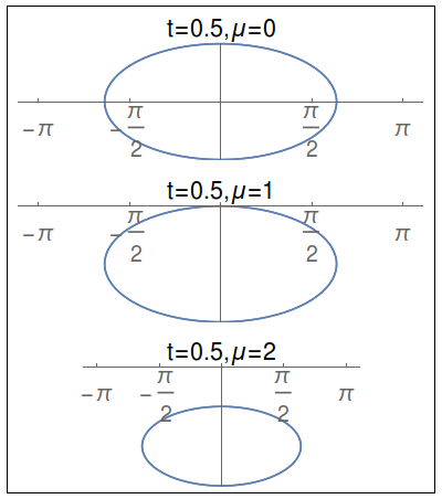
Figure 1: Parametric plots for $\mathcal{H}^{(1)}(k)$ Hamiltonian for different values of $\mu$.

This shows the auxiliary space of the Kitaev chain, which is a closed trajectory with origin inside the curve. The integral along this trajectory takes quantized values indicating the topological quantum phase transition. The value of Zak phase is $\pi$ when the origin is inside the curve of the auxiliary space and 0 when it is outside. Since $\mathcal{H}^{(1)}(k)$ has anti-unitary particle-hole symmetry it gives the reality condition for Majorana representaion matrix ($A(k)^{*}=A(-k)$), i.e.

$$\mathcal{C}A(k)\mathcal{C}^{-1}=A(-k).$$ (17)

This results in the quantized Zak phase which is $0$ for trivial and $\pi$ for non-trivial phases. We verify this by calculating the geometric phase for the system. First we write Kitaev’s chain in momentum space as

$$H_{k}=(\epsilon_{k}-\mu)\sigma_{z}-2\Delta\sin k\sigma_{y}.$$

One can also write the same Hamiltonian in a rotated basis as

$$H_{k}=(\epsilon_{k}-\mu)\sigma_{x}-2\Delta\sin k\sigma_{y},$$ (18)

where $\epsilon_{k}=-2t\cos k$.

$$H_{k}=\begin{bmatrix}0&&(\epsilon_{k}-\mu)\\ (\epsilon_{k}-\mu)&&0\\ \end{bmatrix}-2\Delta\sin k\begin{bmatrix}0&&-i\\ i&&0\\ \end{bmatrix},$$ (19)

$$H_{k}=\begin{bmatrix}0&&(\epsilon_{k}-\mu)+2i\Delta\sin k\\ (\epsilon_{k}-\mu)-2i\Delta\sin k&&0\\ \end{bmatrix},$$ (20)

where $\epsilon_{k}-\mu=r\cos\theta$ and $2\Delta\sin k=r\sin\theta.$ Now the Hamiltonian is reduced to

$$H=\begin{bmatrix}0&&re^{i\theta}\\ re^{-i\theta}&&0\end{bmatrix},$$

where $r=\sqrt{(2t\cos k+\mu)^{2}+4\Delta^{2}\sin^{2}k}$ and   $\theta=-\tan^{-1}(\frac{2\Delta\sin k}{2t\cos k+\mu}).$

Here we are calculating the geometric phase for the lowest-energy eigenfunction. The basic aspects of the geometric phase are given in the appendix. The Berry phase is given by $\gamma_{n}=i\oint\left\langle\Psi_{n}|\nabla_{R}|\Psi_{n}\right\rangle dR,$

where   $\Psi_{n}=\left(\frac{-1}{\sqrt{2}}\right)\left(-e^{i\tan^{-1}(\frac{2\Delta\sin k}{\mu+2t\cos k})}\right),$ and finally the Berry connection is given by

$$A(k)=\left\langle\Psi_{n}|\dfrac{d\Psi_{n}}{dk}\right\rangle=\dfrac{\Delta(2t+\mu\cos k)}{(\mu+2t\cos k)^{2}+4\Delta^{2}\sin^{2}k}.$$

Finally,

$$\gamma_{n}=i\oint Adk=i\oint_{C}\;\;\dfrac{\Delta(2t+\mu\cos(k))}{(\mu+2t\cos(k))^{2}+4\Delta^{2}\sin^{2}(k)}dk.$$ (21)

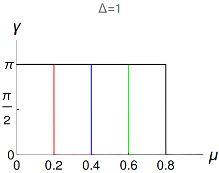
Figure 2: (color online) Variation of $\gamma$ with $\mu$. The red, blue, green, and black curves are for $t$ = 0.1, 0.2, 0.3 and 0.4 respectively.

In fig. 2, we present the variation of geometric phase ($\gamma$) with $\mu$. It is clear from this study that there is a topological quantum phase transition from $\gamma=\pi$ to $\gamma=0$ [34]. We have also observed that the transition occurs at $\mu=2t$ [35].
The physical explanation of this transition can be understood in the following way: Fig. 3 describes the energy dispersion spectrum of this model Hamiltonian, where we observe the gapless state at $k=\pm\pi$. A gapless state is present if the value of the parameters obey the transition relation $\mu=\pm 2t$. This is when transition takes place from topological to non-topological state. If the values of the parameters do not obey the transition relation, then we observe a gapped state (non-topological state), as shown in the lower panel of fig. 3.

Here we clearly observe that the gapless states, in other words degenerate states, appear for discrete values of $\mu$, i.e. $\mu=\pm 2t$ for $k=0$ and $k=\pm\pi$, not for the different values of $\mu$. Thus we justify the topological characterization of the Kitaev chain from the perspective of symmetry Pfaffian number calculation, winding number calculation and also the gapless state at the topological quantum phase transition point.

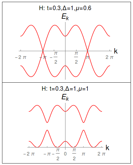
Figure 3: Dispersion curve $E_{k}$ vs k for the Hamiltonian $\mathcal{H}^{(1)}(k)$.

Results and discussion for the Hamiltonian $\mathcal{H}^{(2)}(k)$ : The Hamiltonian $\mathcal{H}^{(2)}(k)$ in the matrix form can be written as

$$\mathcal{H}^{(2)}(k)=\left(\begin{matrix}-2t\cos(k)-\mu&&2i\Delta\sin(k)+i\alpha k\\ -2i\Delta\sin(k)-i\alpha k&&2t\cos(k)+\mu\end{matrix}\right).$$ (22)

Here we consider three variants of Kitaev chain in momentum space. One can express the Kitaev chain in the basis of $\sigma_{x}$ and $\sigma_{y}$. The present study is only for the theoretical exercise over the Kitaev chain. But it has some interesting physics that all these variants of Kitaev chain ($\mathcal{H}^{(2)}(k),\mathcal{H}^{(3)}(k),\mathcal{H}^{(4)}(k)$) are hermitian in character. Upon adding of the $\alpha k$ term, either in $\sigma_{x}$ or $\sigma_{y}$, the two components of the Kitaev chain, we observe very interesting results from the perspective of different topological symmetry classes of the auxiliary space and the condition for topological characterization. The pairing mechanism of the Kitaev chain in real space is the well-defined p-wave pairing mechanism. But for the other three model Hamiltonians ($\mathcal{H}^{(2)}(k),\mathcal{H}^{(3)}(k),\mathcal{H}^{(4)}(k)$), we do not know the nature of the interaction. We consider these model Hamiltonians for the complete theoretical interest and at the same time they satisfy the hermiticity property of the Hamiltonian and also one can express these model Hamiltonians into two different symmetry classes (BDI and AIII). Kitaev’s model belongs to the BDI symmetry class. Therefore the present study has relevence from the perspective of symmetry class. We would like to study how the symmetry and topological properties are modified in the presence of additional terms. Therefore we present an extensive study from the perspective of topological symmetry class in momentum space.
Many studies in theoretical physics do not find proper physical justification at the very beginning. But in due course of time, they are justified. The new and important results of this study may motivate quantum simulation physicists to quantum-simulate this system.
This model Hamiltonian satisfies the conditions for time-reversal, particle-hole and chiral symmetry operations,

$$\mathcal{T}\mathcal{H}^{(2)}(k)\mathcal{T}^{-1} ={K}\mathcal{H}^{(2)}(k){K}^{-1}$$ (23)

$$=\hat{K}\left(\begin{matrix}-2t\cos(k)-\mu&&2i\Delta\sin(k)+i\alpha k\\ -2i\Delta\sin(k)-i\alpha k&&2t\cos(k)+\mu\\ \end{matrix}\right)\hat{K}$$

$$=\mathcal{H}^{(2)}(k),$$

$$\mathcal{C}\mathcal{H}^{(2)}(k)\mathcal{C}^{-1} =(\sigma_{x}{K})\mathcal{H}^{(2)}(k)(\sigma_{x}{K})^{-1}$$ (24)

$$=\left(\begin{matrix}0&&1\\ 1&&0\\ \end{matrix}\right)\left(\begin{matrix}-2t\cos(k)-\mu&&2i\Delta\sin(k)+i\alpha k\\ -2i\Delta\sin(k)-i\alpha k&&2t\cos(k)+\mu\\ \end{matrix}\right)\left(\begin{matrix}0&&1\\ 1&&0\\ \end{matrix}\right)$$

$$=-\mathcal{H}^{(2)}(k),$$

$$\mathcal{S}\mathcal{H}^{(2)}(k)\mathcal{S}^{-1} =\sigma_{x}\mathcal{H}^{(2)}(k)\sigma_{x}^{-1}$$ (25)

$$=\left(\begin{matrix}0&&1\\ 1&&0\\ \end{matrix}\right)\left(\begin{matrix}-2t\cos(k)-\mu&&2i\Delta\sin(k)+i\alpha k\\ -2i\Delta\sin(k)-i\alpha k&&2t\cos(k)+\mu\\ \end{matrix}\right)\left(\begin{matrix}0&&1\\ 1&&0\\ \end{matrix}\right)$$

$$=-\mathcal{H}^{(2)}(k).$$

Thus we have

$$\mathcal{T}\mathcal{H}^{(2)}(k)\mathcal{T}^{-1}=\mathcal{H}^{(2)}(k),\;\;\;\mathcal{C}\mathcal{H}^{(2)}(k)\mathcal{C}^{-1}=-\mathcal{H}^{(2)}(k),$$

$$\mathcal{S}\mathcal{H}^{(2)}(k)\mathcal{S}^{-1}=-\mathcal{H}^{(2)}(k).$$ (26)

As in the case of Kitaev chain ($\mathcal{H}^{(1)}(k)$), $\mathcal{H}^{(2)}(k)$ also belongs to the symmetry class BDI [6] with the topological invariant $\mathbb{Z}$ (see table 1). One can also expect the topological quantum phase transition in $\mathcal{H}^{(2)}(k)$. This system has anti-unitary particle-hole symmetry, thus one may consider that the system is in the topological state and Zak phase must be quantized [7, 13]. But we observe that even though the symmetry class of the Hamiltonian $\mathcal{H}^{(1)}(k)$ and $\mathcal{H}^{(2)}(k)$ are the same, there is no topological non-trivial phase for these model Hamiltonians. Addition of the term $\alpha k$ breaks the anti-symmetric property of the Majorana representation matrix for $k=\pi$,

$${\small A(\pi)=\left(\begin{matrix}0&&2t-\mu+i\alpha\pi\\ -2t+\mu+i\alpha\pi&&0\\ \end{matrix}\right).}$$ (27)

For this case one cannot calculate the Majorana number since the Pfaffian does not exist due to lack of the anti-symmetric property. This also indicates that there is no topological non-trivial phase for this system. This result is also evident from the nature of auxiliary space of $\mathcal{H}^{(2)}(k)$.

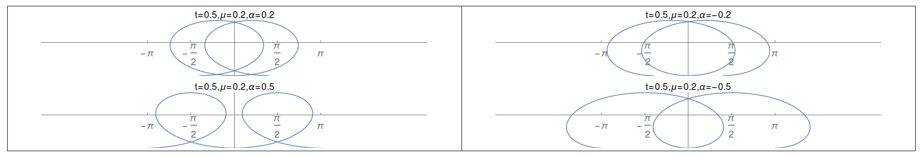
Figure 4: Parametric plots for $\mathcal{H}^{(2)}(k)$ for different values of $\mu$, $\alpha$ and $t$.

Fig. 4 shows that the trajectory in the auxiliary space is not closed and the integral along the trajectory will not take quantized values. We observe an interesting feature from this behaviour in the auxiliary space that, although the origin of auxiliary space is encircled by the curve, the system is in the non-topological state. At the same time there is no mirror symmetry with $\alpha$. This can also be verified from the energy dispersion curve (fig. 5). It shows there is no gapless state for topological quantum phase transition to occur. The Hamiltonian $\mathcal{H}^{(2)}(k)$ does not have the mirror-symmetric auxiliary space curves for positive and negative values of $\alpha$.

It is clear from this section that even though both the Hamiltonians $\mathcal{H}^{(1)}(k)$ and $\mathcal{H}^{(2)}(k)$ belong to the BDI symmetry class they have different topological properties. In the case of $\mathcal{H}^{(2)}(k)$ there is no topological non-trivail phase as expected for the BDI symmetry class. Majorana representation matrix is anti-symmetric for $\mathcal{H}^{(1)}(k)$ while it does not satisfy this condition for $\mathcal{H}^{(2)}(k)$. Thus it is not possible to calculate topological invariant to characterize the topological state for $\mathcal{H}^{(2)}(k)$. Energy dispersion for $\mathcal{H}^{(1)}(k)$ is gapless, while for $\mathcal{H}^{(2)}(k)$ there is no gapless dispersion, indicating there is no topological phase transition for $\mathcal{H}^{(2)}(k)$. Auxiliary space curve also gives the same conclusion. It is closed curve for $\mathcal{H}^{(1)}(k)$, indicating integer topological invariant. In the case of $\mathcal{H}^{(2)}(k)$ it is open curve, which shows the absence of topological non-tivial phase. Thus it is clear from this study that the same symmetry class does not reveal the same topological properties.

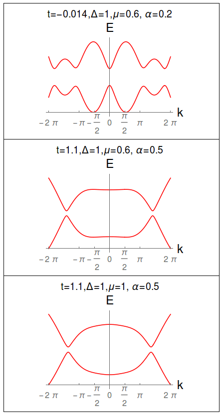
Figure 5: Dispersion curve of $E_{k}$ vs k for the $\mathcal{H}^{(2)}(k)$ Hamiltonian.

Results and discussion for the Hamiltonians of AIII symmetry class
Here we present the results for Hamiltonians $\mathcal{H}^{(3)}(k)$ and $\mathcal{H}^{(4)}(k)$. The matrix form of the Hamiltonian $\mathcal{H}^{(3)}(k)$ can be written as

$$\mathcal{H}^{(3)}(k)=\left(\begin{matrix}-2t\cos(k)-\mu-\alpha k&&2i\Delta\sin(k)\\ -2i\Delta\sin(k)&&2t\cos(k)+\mu+\alpha k\\ \end{matrix}\right).$$ (28)

We observe that $\mathcal{H}^{(3)}(k)$ does not satisfy the condition for time-reversal and particle-hole symmetry operations but satisfies only the chiral symmetry condition.

$$\mathcal{T}\mathcal{H}^{(3)}(k)\mathcal{T}^{-1} ={K}\mathcal{H}^{(3)}(k){K}^{-1}$$ (29)

$$=\hat{K}\left(\begin{matrix}-2t\cos(k)-\mu-\alpha k&&2i\Delta\sin(k)\\ -2i\Delta\sin(k)&&2t\cos(k)+\mu+\alpha k\\ \end{matrix}\right)\hat{K}$$

$$\neq\mathcal{H}^{(3)}(k),$$

$$\mathcal{C}\mathcal{H}^{(3)}(k)\mathcal{C}^{-1} =(\sigma_{x}{K})\mathcal{H}^{(3)}(k)(\sigma_{x}{K})^{-1}$$ (30)

$$=\left(\begin{matrix}0&&1\\ 1&&0\\ \end{matrix}\right)\left(\begin{matrix}-2t\cos(k)-\mu+\alpha k&&2i\Delta\sin(k)\\ -2i\Delta\sin(k)&&2t\cos(k)+\mu-\alpha k\\ \end{matrix}\right)\left(\begin{matrix}0&&1\\ 1&&0\\ \end{matrix}\right)$$

$$\neq-\mathcal{H}^{(3)}(k),$$

$$\mathcal{S}\mathcal{H}^{(3)}(k)\mathcal{S}^{-1} =(\sigma_{x})\mathcal{H}^{(3)}(k)(\sigma_{x})^{-1}$$ (31)

$$=\left(\begin{matrix}0&&1\\ 1&&0\\ \end{matrix}\right)\left(\begin{matrix}-2t\cos(k)-\mu-\alpha k&&i2\Delta\sin(k)\\ -i2\Delta\sin(k)&&2t\cos(k)+\mu+\alpha k\\ \end{matrix}\right)\left(\begin{matrix}0&&1\\ 1&&0\\ \end{matrix}\right)$$

$$=-\mathcal{H}^{(3)}(k).$$

Thus we have

$$\mathcal{T}\mathcal{H}^{(3)}(k)\mathcal{T}^{-1}\neq\mathcal{H}^{(3)}(k)\;\;\;\mathcal{C}\mathcal{H}^{(3)}(k)\mathcal{C}^{-1}\neq-\mathcal{H}^{(3)}(k),$$

$$\mathcal{S}\mathcal{\mathcal{missing}}{H}^{(3)}(k)\mathcal{S}^{-1}=-\mathcal{\mathcal{missing}}{H}^{(3)}(k).$$ (32)

Thus, from the symmetry analysis, $\mathcal{H}^{(3)}(k)$ falls under AIII class in the ten symmetry classes with topological invariant number $\mathbb{Z}$. This indicates that there is a possibility for the topological quantum phase transition by tuning the parameters to obtain the gapless state with the change in the topological invariant number $\mathbb{Z}$. But we observe a strange behaviour of the system, that it does not allow one to calculate Majorana number $\mathcal{M}$ (eq. 15) to get the condition for the parameters. The Majorana representation matrix $A_{\alpha\beta}$ for $\mathcal{H}^{(3)}(k)$ is given by

$${\small A(k)=\left(\begin{matrix}0&&\xi_{k}+\alpha k+i2\Delta\sin k\\ -\xi_{k}+\alpha k+i2\Delta\sin k&&0\\ \end{matrix}\right),}$$ (33)

where $\xi_{k}=-2t\cos k-\mu$. Here $A(k)$ loses the anti-symmetric property for $k=\pi$, which does not allow one to calculate the Pfaffian of the matrix. This indicates that there is no Majorana number, which implies that the system is in non-trivial topological phase. This can also be verifed by the trajectory of the system in the auxiliary space, given in fig. 6.

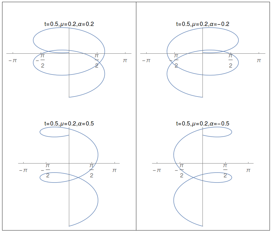
Figure 6: Parametric plots for $\mathcal{H}^{(3)}(k)$ for different values of $\mu$, $\alpha$ and $t$.

A very interesting observation can be made from fig. 6: although the auxiliary space curve in the upper panel encircles the origin, the curve is not closed. For the system to be in the topological state, the auxiliary space curve encirling the origin is a necessary condition, but the closedness of the curve is the sufficient condition, as we observe in the Kitaev chain (fig. 1). The left and the right panels represent the auxiliary space curves for positive and negative values of $\alpha$. They show mirror-symmetric behaviour for positive and negative values of $\alpha$. Although the auxiliary space curve is symmetric with respect to positive and negative values of $\alpha$, it is not symmetric with respect to $k$. Thus we conclude that the topological properties of the system do not depend on the symmetry of the auxiliary space.

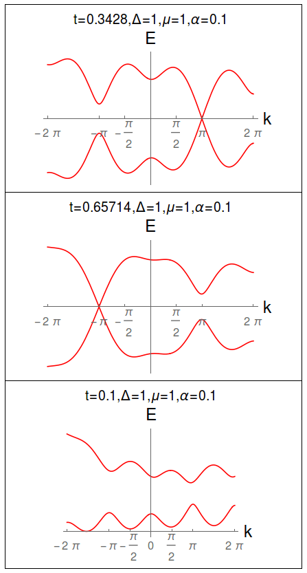
Figure 7: Dispersion curve of $E_{k}$ vs k for the Hamiltonian $\mathcal{H}^{(3)}(k)$.

We observe that there is no closed trajectory in the auxiliary space. We also observe that the addition of $\alpha k$ to Hamiltonian $\mathcal{H}^{(3)}(k)$ results in breaking of the periodicity of the Brillouin zone. One can observe this from energy dispersion curve (fig. 7) that $E(\pi)\neq E(-\pi)$. This lack of periodicity does not allow one to calculate the geometric/Zak phase [7, 13]. In other words the integral over the non-periodic Brillouin zone will not be a Cauchy integral and does not take the quantized value [39], which again indicates that there is no topological quantum phase transition. We discuss this in the next section.

Results and discussion for the Hamiltonian $\mathcal{H}^{(4)}(k)$ : The matrix form of the Hamiltonian $\mathcal{H}^{(4)}(k)$ is given by

$$\mathcal{H}^{(4)}(k)=\left(\begin{matrix}-2t\cos(k)-\mu-\alpha_{1}k&&2i\Delta\sin(k)+i\alpha_{2}k\\ -2i\Delta\sin(k)-i\alpha_{2}k&&2t\cos(k)+\mu+\alpha_{1}k\\ \end{matrix}\right).$$ (34)

We observe that $\mathcal{H}^{(4)}(k)$ belongs to the symmetry class AIII, i.e. it only obeys the chiral symmetry condition.

$$\mathcal{T}\mathcal{H}^{(4)}(k)\mathcal{T}^{-1} ={K}\mathcal{H}^{(4)}(k){K}^{-1}$$ (35)

$$=\hat{K}\left(\begin{matrix}-2t\cos(k)-\mu-\beta_{1}k&&2i\Delta\sin(k)+i\beta_{2}k\\ -2i\Delta\sin(k)-i\beta_{2}k&&2t\cos(k)+\mu+\beta_{1}k\\ \end{matrix}\right)\hat{K}$$

$$\neq\mathcal{H}^{(4)}(k),$$

$$\mathcal{C}\mathcal{H}^{(4)}(k)\mathcal{C}^{-1} =(\sigma_{x}\hat{K})\mathcal{H}^{(4)}(k)(\sigma_{x}{K})^{-1}$$ (36)

$$=\left(\begin{matrix}0&&1\\ 1&&0\\ \end{matrix}\right)\left(\begin{matrix}-2t\cos(k)-\mu+\beta_{1}k&&2i\Delta\sin(k)+i\beta_{2}k\\ -2i\Delta\sin(k)-i\beta_{2}k&&2t\cos(k)+\mu-\beta_{1}k\\ \end{matrix}\right)\left(\begin{matrix}0&&1\\ 1&&0\\ \end{matrix}\right)$$

$$\neq-\mathcal{H}^{(4)}(k),$$

$$\mathcal{S}\mathcal{H}^{(4)}(k)\mathcal{S}^{-1} =(\sigma_{x})\mathcal{H}^{(4)}(k)(\sigma_{x})^{-1}.$$ (37)

$$=\left(\begin{matrix}0&&1\\ 1&&0\\ \end{matrix}\right)\left(\begin{matrix}-2t\cos(k)-\mu-\beta_{1}k&&2i\Delta\sin(k)+i\beta_{2}k\\ -2i\Delta\sin(k)-i\beta_{2}k&&2t\cos(k)+\mu+\beta_{1}k\\ \end{matrix}\right)\left(\begin{matrix}0&&1\\ 1&&0\\ \end{matrix}\right)$$

$$=-\mathcal{H}^{(4)}(k).$$

Thus we have

$$\mathcal{T}\mathcal{H}^{(4)}(k)\mathcal{T}^{-1}\neq\mathcal{H}^{(4)}(k),\;\;\;\mathcal{C}\mathcal{H}^{(4)}(k)\mathcal{C}^{-1}\neq-\mathcal{H}^{(4)}(k),$$

$$\mathcal{S}\mathcal{H}^{(4)}(k)\mathcal{S}^{-1}=-\mathcal{H}^{(4)}(k).$$ (38)

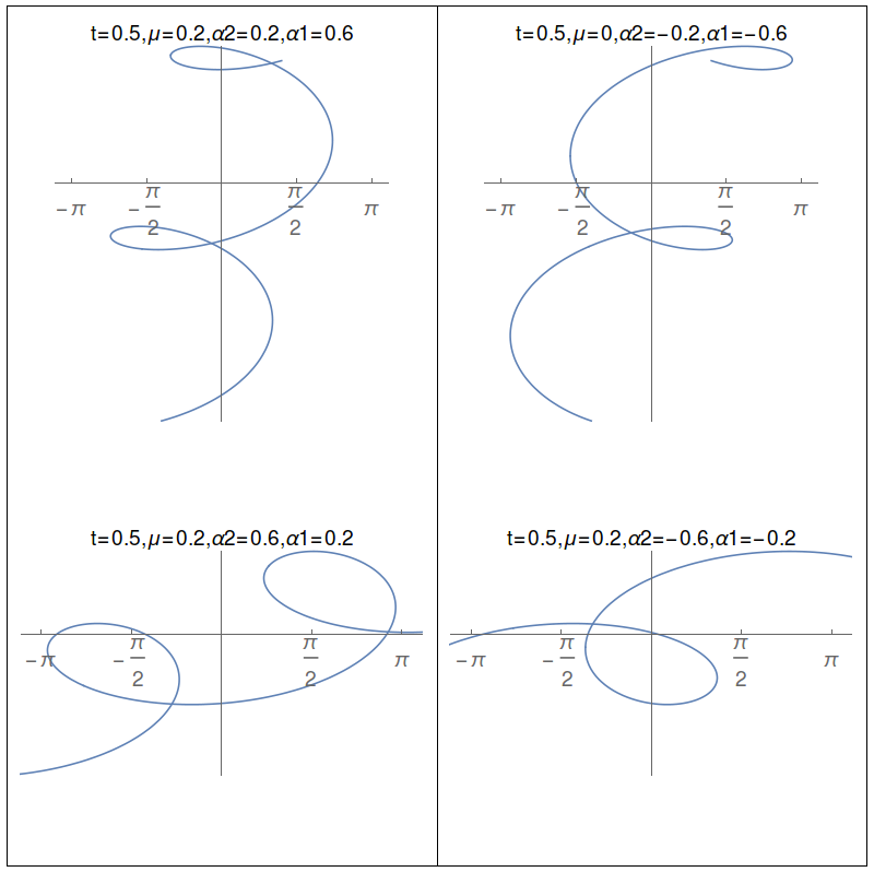
Figure 8: Parametric plots for $\mathcal{H}^{(4)}(k)$ for different values of $\mu$, $\alpha$ and $t$.

Thus Hamiltonian $\mathcal{H}^{(4)}(k)$ also falls under the same symmetry class as $\mathcal{H}^{(3)}(k)$ i.e. AIII symmetry class. Here also one can expect the topological quantum phase transition with change in the value of topological invariant number $\mathbb{Z}$. But similar to $\mathcal{H}^{(2)}(k)$ and $\mathcal{H}^{(3)}(k)$, we observe the Majorana representation matrix breaks its anti-symmetric property as we add the $\alpha k$ term,

$${\small A(\pi)=\left(\begin{matrix}0&&2t-\mu+\alpha_{1}\pi+i\alpha_{2}\pi\\ -2t+\mu+\alpha_{1}\pi+i\alpha_{2}\pi&&0\\ \end{matrix}\right).}$$ (39)

Thus Pfaffian does not exist for this system, which shows there is no topological non-trivial phase.

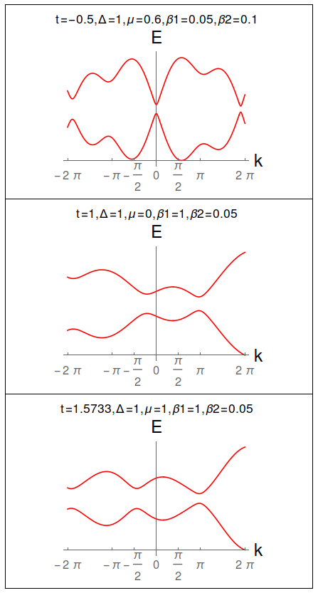
Figure 9: Dispersion curve of $E_{k}$ vs k for the $H^{(4)}(k)$ Hamiltonian.

Here the trajectory in the auxiliary space is not closed and integral along the trajectory is not quantized. Absence of the origin inside the perimeter of the trajectory in fig. 8 shows there is no topological state for the system. The curves in the auxiliary space are neither symmetric with $\alpha$ nor with $k$. A curve in the auxiliary space encircling the origin is a necessary condition but the closedness of the curve is the sufficient condition for the system to be in the topological state. This can also be verified from fig. 9, which shows the energy dispersion for $\mathcal{H}^{(4)}(k)$. We observe that there are no gapless states responsible for topological quantum phase transition.

It is clear from this section that both the Hamiltonians $\mathcal{H}^{(3)}(k)$ and $\mathcal{H}^{(4)}(k)$ belong to the symmetry class AIII. They are expected to get the topological non-trivial phase for this symmetry class but both the Hamiltonians do not show any property indicating the presence of topological non-trivial phase. Majorana representaion matrix does not show anti-symmetric property, and auxiliary space curve is not closed and thus shows there is no possibility of having topological non-trivial phase.

A Comparision of Results for two different symmetry classes :
We have noticed in the BDI symmetry class that the topological behaviour of the Hamiltonians $\mathcal{H}^{(1)}(k)$ and $\mathcal{H}^{(2)}(k)$ are different. The Kitaev Hamiltonian $\mathcal{H}^{(1)}(k)$ shows the topological phase transition while there is no topological phase transition for $\mathcal{H}^{(2)}(k)$. It results from the dispersion curve, which for $\mathcal{H}^{(1)}(k)$ shows a gapless state indicating the transition point. But for BDI symmetry-class Hamiltonians obey $\mathcal{H}(k=-\pi)=\mathcal{H}(k=\pi)$, while for the case of AIII symmetry $\mathcal{H}(k=-\pi)\neq\mathcal{H}(k=\pi)$. We also observe that there is no closing of the gap at both $k=\pm\pi$, as we find for $\mathcal{H}^{(1)}(k)$ dispersion. The energy dispersion for $\mathcal{H}^{(3)}(k)$ and $\mathcal{H}^{(4)}(k)$ are different although these two belong to the same symmetry class. Thus it is clear from this study of two different symmetry classes that gap closedness is the prime condition to get topological quantum phase transition of the system.

A Few Relevant Calculations and Discussion for the Topological Characterization of these two symmetry classes - BDI and AIII.

(A). A derivation for sufficient condition for topological characterization from the behaviour of curves in auxiliary space.

Here we mathematically prove the sufficient condition for the topological characterization of the system from the behaviour of auxiliary space. We have

$$\mathcal{H}^{(3)}(k)=(-2t\cos k-\mu+\alpha_{1}k)\sigma_{x}+(\alpha_{2}k-2\Delta\sin k)\sigma_{y}.$$ (40)

We plot the parametric plot $(x(k),y(k))$,

$$x(k)=-2t\cos k-\mu+\alpha_{1}k=r(k)\cos\theta(k),$$ (41)

$$y(k)=\alpha_{2}k-2\Delta\sin k=r(k)\sin\theta(k),$$ (42)

so that, in the auxiliary plane,

$$r^{2}(k)=(-2t\cos k-\mu+\alpha_{1}k)^{2}+(\alpha_{2}k-2\Delta\sin k)^{2},$$ (43)

$$\theta(k)=\tan^{-1}\left[\frac{\alpha_{2}k-2\Delta\sin k}{-2t\cos k-\mu+\alpha_{1}k}\right].$$ (44)

To have a closed curve for $k$ running between $\left[-\pi,\pi\right]$ the curve must come back to its starting point, i.e.

$$r^{2}(k=\pi)=r^{2}(k=-\pi),\;\;\;\;\theta(k=\pi)=\theta(k=-\pi)\;\;mod(2\pi).$$ (45)

Putting these two conditions in the expression of $r^{2}(k)$ and $\theta(k)$,

$$(-2t\cos(-\pi)-\mu+\alpha_{1}(-\pi))^{2}+(\alpha_{2}(-\pi)-2\Delta\sin(-\pi))^{2}=(-2t\cos(\pi)-\mu+\alpha_{1}(\pi))^{2}+(\alpha_{2}(\pi)-2\Delta\sin(\pi))^{2},$$ (46)

and

$$\tan^{-1}\left[\frac{\alpha_{2}(-\pi)-2\Delta\sin(-\pi)}{-2t\cos(-\pi)-\mu+\alpha_{1}(-\pi)}\right]=\tan^{-1}\left[\frac{\alpha_{2}(\pi)-2\Delta\sin(\pi)}{-2t\cos(\pi)-\mu+\alpha_{1}(\pi)}\right].$$ (47)

The conditions for the curve to be closed, i.e. eq. 46 and eq. 47, can be simultaneously satisfied if $\alpha_{1}=\alpha_{2}=0$. Thus it is clear from this study that this equation ($\alpha_{1}=0=\alpha_{2})$ is only satisfied by the Hamiltonian $\mathcal{H}^{(1)}(k)$, i.e. Kitaev chain.
Therefore it is clear from this study that the addition of $\alpha k$ term either in $\sigma_{x}$ or $\sigma_{y}$ components or both does not favour the existence of the topological state of matter. The field of quantum simulation physics is rich and it has application in different branches of physics [7, 26]. Our strong belief is that this result motivates quantum simulation physicists to find this behaviour in different physical systems. To the best of our knowledge this study is the first in the literature to study the necessary and sufficient conditions for topological characterization from the behaviour of auxiliary space.

(B). A general physical explanation for the existence of topological state: from the perspective of Berry connection and geometric phase.

BdG Hamiltonian obeys an anti-unitary particle-hole symmetry, $\mathcal{C}=\sigma_{x}K$ ($\sigma_{x}$ and $K$ are Pauli spin matrix and complex conjugate operator respectively.),

$$\left\{\mathcal{H}_{BdG},\mathcal{C}\right\},$$ (48)

with $\mathcal{C}^{2}=1$. This symmetry implies that the bands below and above the energy gap are conjugates of each other, i.e.

$$\mathcal{C}\ket{\Psi^{o}(-k)}=e^{-i\phi(k)}\ket{\Psi^{e}(-k)}.$$ (49)

Here $\ket{\Psi^{o}}$ and $\ket{\Psi^{e}}$ are the Bloch states of the occupied and empty bands respectively. Using this abelian Berry connection [40, 41] of the occupied bands can be written as

$$\mathcal{A}^{o}(k)=-i\sum_{\alpha}\bra{\psi^{o}_{\alpha}(k)}\partial_{k}\ket{\psi^{o}_{\alpha}(k)},$$ (50)

where $\alpha=1,...,n$ represent the independent Bloch bands. One can observe the equivalence of the Berry connection of the occupied bands at $k$ and the empty bands at $-k$ up to a gauge transformation,

$$\mathcal{A}^{o}(-k)=\mathcal{A}^{e}(k)-\sum_{\alpha}\partial_{k}\phi_{\alpha}(k).$$ (51)

This constraint implies that the Zak phase over half of the Brillouin zone can be written as

$$\gamma=\int\limits_{-\pi}^{\pi}\mathcal{A}^{o}(k)dk=\int\limits_{0}^{\pi}\left[\mathcal{A}(k)-\partial_{k}\phi(k)\right]dk,$$ (52)

with $\mathcal{A}(k)=\mathcal{A}^{o}(k)+\mathcal{A}^{e}(k)$. In the Majorana representation one can write the $\mathcal{H}_{BdG}$ in diagonal form as

$$W(k)\mathcal{H}_{BdG}W^{\dagger}(k)=\sigma_{z}diag(\epsilon_{\lambda}),$$ (53)

where from the particle-hole symmetry $W$ safisfies the condition

$$\mathcal{C}W(k)\mathcal{C}^{-1}=W(-k).$$ (54)

This implies that the phase factor $\phi(k)$ in eq. 52 vanishes. Thus in the presence of anti-unitary particle-hole symmetry the Zak phase is quantized to integer multiples of $\pi$, indicating the gapless state with topological quantum phase transition.

But for the present case, in presence of $\alpha k$ term, one cannot express the Berry connection $\mathcal{A}^{0}(-k)$ to $\mathcal{A}^{e}(k)$ by eq. 51 and also geometric phase, $\gamma$, as in eq. 52.

C. Topological characterization from the perspective of winding number

In general BdG Hamiltonian in the symmetry class BDI can be written in the special form as

$$\mathcal{H}^{(1)}(k)=\left(\begin{matrix}h_{0}(k)&&i\Delta(k)\\ -i\Delta(k)&&-h_{0}(k)\end{matrix}\right).$$ (55)

This can be written in the diagonal form as

$$\mathcal{H}^{(1)}(k)=\left(\begin{matrix}0&&A(k)\\ A^{T}(-k)&&0\end{matrix}\right),$$ (56)

where $A(k)=h_{0}(k)+i\Delta(k)$, satisfying the condition $A^{*}(k)=A(-k)$. Winding number in this case can be defined from the phase of $A(k)$,

$$A(k)=|A(k)|e^{i\theta(k)}.$$ (57)

Considering $z(k)=e^{i\theta(k)}$ one can define the winding number as

$$w=\frac{-i}{\pi}\int\limits_{0}^{\pi}\frac{dz(k)}{z(k)}=\frac{1}{\pi}(\theta(\pi)-\theta(0)).$$ (58)

In the case of Kitaev chain, i.e. $\mathcal{H}^{(1)}(k)$, we have

$$|A(k)|=\sqrt{(2t\cos k+\mu)^{2}+(2\Delta\sin k)^{2}},$$ (59)

$$\theta(k)=\tan^{-1}\left[\frac{2\Delta\sin k}{-2t\cos k-\mu}\right].$$ (60)

Thus the winding number for Kitaev chain is given by

$$w=\frac{1}{\pi}(\pi-0)=1.$$ (61)

Since $\tan^{-1}(0)$ can be either $0$ or $\pi$, winding number can take quantized values, $w=\pm 1,0$.

In the case of $\mathcal{H}^{(2)}(k)$, $\mathcal{H}^{(3)}(k)$ and $\mathcal{H}^{(4)}(k)$ one cannot define the integral in eq. 58. Even if we try to calculate the winding by brute force for $\mathcal{H}^{(4)}(k)$, then we have

$$\theta(k)=\tan^{-1}\left[\frac{2\Delta\sin k+\alpha_{2}k}{-2t\cos k-\mu+\alpha_{1}k}\right].$$ (62)

The winding number is given by

$$w =\frac{1}{\pi}\left(\tan^{-1}\left(\frac{\alpha_{2}\pi}{2t-\mu+\alpha_{1}k}\right)-0\right)$$ (63)

$$=\frac{1}{\pi}\tan^{-1}\left(\frac{\alpha_{2}\pi}{2t-\mu+\alpha_{1}k}\right).$$

We observe that the winding number is not quantized to integer values but takes continuous values, thus the system will be in non-topological state for all non-zero values of $\alpha_{1}$ and $\alpha_{2}$.

Conclusions:

We have presented the results of symmetry, topology and quantization of geometric phase along with the physical explanation for two different topological symmetry classes. The nature of these model Hamiltonians and the results should motivate quantum simulation physics to simulate these types of model Hamiltonian in different physical systems. We have shown explicitly that the symmetry criteria are not sufficient to characterize the topological state of the systems. We have also presented the results based on auxiliary space to derive the necessary and sufficient conditions for topological characterization.

Acknowledgments
The authors would like to acknowledge DST (EMR/2017/000898) for the funding and Raman Research Institute library for the books and journals. The authors would like to acknowledge Mr.N.A.Prakash for critical reading of this manuscript. Finally authors would like to acknowledge International Centre for Theoretical Sciences Lectures/seminars/workshops /conferences/discussion meetings on different aspects of physics.

Appendix

Berry phase in Bloch band

The basic Hamiltonian for the Bloch band can be written as $H=\frac{k^{2}}{2m}+V(r)$, with the value $V(r+a)=V(r)$, where $a$ is the distance between two lattice points. The Bloch state satisfies the following conditions for the edge state: $\psi_{nK}(r+a)=e^{iq.a}\psi_{nk}(r)$, i.e. the wavefunction at the points $r$ and $r+a$ are related to the phase. One can also write the model Hamiltonian as $H(q)=\frac{(k+\hbar q)^{2}}{2m}+V(r),$ and the wavefunction

$$\psi_{nq}(r)=u_{nq}(r)e^{iq.r},$$

where $u_{nq}(r)$ is the free particle wavefunction in the presence of periodic potential, which also satisfies the following condition:

$$u_{nq}(r+a)=u_{nq}(r).$$

The most interesting point to be noted is the Brillouin zone in the parameter space for the transformed Hamiltonian with the eigen basis $|u_{nq}\rangle$. The states $|\psi_{n}(q)\rangle$ and $|\psi_{n}(q+h)\rangle$ satisfy the same boundary condition as that of the torus. The crystal momentum q is found to vary and the Bloch state picks up a Berry phase. This is nothing but the Zak phase

$$\gamma_{n}=\oint dq.\langle u_{n}(q)|i\Delta_{q}|u_{n}(q)\rangle.$$

For the Kitaev chain (Hamiltonian $\mathcal{H}^{(1)}(k)$) the physics is all right, but in the presence of $\alpha k$ term the wavefunction

$$|\psi_{n}(q)\rangle\neq|\psi_{n}(q+h)\rangle,$$

and the parameter of the Zak phase is not valid.

References

[1]
Duncan Haldane (Nobel Prize in Physics 2016), Distinguished lecture on 11 January 2019 at ICTS, India.
[2]
Chiu, Ching-Kai and Teo, Jeffrey C. Y. and Schnyder, Andreas P. and Ryu, Shinsei. Rev. Mod. Phys. 88 (2016) 035005.
[3]
M. Z. Hasan and C. L. Kane. Rev. Mod. Phys. 82 (2010) 3045.
[4]
Masatoshi Sato and Yoichi Ando. Reports on Progress in Physics. 80 (2017) 076501.
[5]
Ching-Kai Chiu, Jeffrey C. Y. Teo, Andreas P. Schnyder, and Shinsei Ryu. Reviews of Modern Physics. 88 (2016) 035005.
[6]
Alexander Altland and Martin R. Zirnbauer. Phys. Rev. B, 55 (1997) 1142–1161.
[28]
Georgescu, IM and Ashhab, Sahel and Nori, Franco. Reviews of Modern Physics, 86(1) (2014) 153.
[29]
Florian Loder, Arno P Kampf, and Thilo Kopp. Journal of Physics: Condensed Matter, 25(36) (2013) 362201.
[30]
Dario Bercioux and Procolo Lucignano. Reports on Progress in Physics, 78(10) (2015) 106001.
[31]
A. Manchon, H. C. Koo, J. Nitta, S. M. Frolov, and R. A.. Duine. Nature Materials, 14 (2015) 871–882.
[32]
A Yu Kitaev. Physics-Uspekhi, 44(10S) (2001) 131.
[33]
Jan Carl Budich and Eddy Ardonne. Physical Review B, 88 (2013) 075419.
[34]
A. Alexandradinata and B. Andrei Bernevig. Phys. Rev. B, 93 (2016) 205104.
[35]
Kai Sun. Lecture Notes (2012).
[36]
Suhas Gangadharaiah, Jianmin Sun, and Oleg A Starykh. Physical Review B, 78(5) (2008) 054436.
[37]
Jairo Sinova, Dimitrie Culcer, Q Niu, NA Sinitsyn, T Jungwirth, and
AH MacDonald. Physical Review Letters, 92(12) (2004) 126603.
[38]
FE Meijer, AF Morpurgo, and TM Klapwijk. Physical Review B, 66(3) (2002) 033107.
[39]
Ablowitz, M.J. and Fokas, A.S. Cambridge Texts in Applied Mathematics (2003).
[40]
Hong, SP and Doh, H and Salk, SH. arXiv preprint quant-ph/9605040 (1996).
[41]
Pachos, Jiannis K and Carollo, Angelo CM. Philosophical Transactions of the Royal Society of London A: Mathematical, Physical and Engineering Sciences, 364(1849) (2006) 3463–3476.