Analysis and entropy stability of the line-based discontinuous Galerkin method

Abstract.

We develop a discretely entropy-stable line-based discontinuous Galerkin method for hyperbolic conservation laws based on a flux differencing technique. By using standard entropy-stable and entropy-conservative numerical flux functions, this method guarantees that the discrete integral of the entropy is non-increasing. This nonlinear entropy stability property is important for the robustness of the method, in particular when applied to problems with discontinuous solutions or when the mesh is under-resolved. This line-based method is significantly less computationally expensive than a standard DG method. Numerical results are shown demonstrating the effectiveness of the method on a variety of test cases, including Burgers’ equation and the Euler equations, in one, two, and three spatial dimensions.

1. Introduction

High-order numerical methods for the solution of partial differential equations have seen success in a wide range of application areas [42]. In particular, the discontinuous Galerkin (DG) method [8, 34], an arbitrary-order finite element method suitable for use on unstructured geometries, possesses many desirable properties, making it well-suited for a large number of applications. Variants of the DG method, such as the discontinuous Galerkin spectral element method (DG-SEM) [1, 32, 20] and the line-based discontinuous Galerkin method (Line-DG) [28, 29] have been introduced in order to retain the attractive properties of the DG method while reducing its computational cost.

Of particular interest are the stability properties of these methods. It has been shown that the standard discontinuous Galerkin method satisfies a cell entropy inequality in the scalar and symmetric system case, leading to $L^{2}$ stability [18, 15]. However, these results do not immediately translate to general systems of conservation laws. Additionally, these results rely on the use of exactly integrated DG methods, which may be impractical or prohibitively expensive due to nonlinearities in the fluxes. To maintain stability in the general nonlinear case, a variety of methods have been proposed, including limiters [45, 9] and artificial viscosity [30, 46], however these methods can result in reduced order of accuracy, and often require parameter tuning. Recently, discretely entropy-stable DG and DG-SEM methods have been developed based on a technique known as flux differencing [4, 7, 3, 11, 13, 12, 24]. These methods are based on the entropy-conservative and entropy-stable fluxes developed by Tadmor [38, 37, 23], which have been used in the context of finite volume methods.

In this work, we extend the flux differencing methodology to the line-based DG (Line-DG) methods developed in [28, 29]. These methods are closely related both to standard DG methods and to DG-SEM methods, and are based on solving a sequence of one-dimensional Galerkin problems along lines of nodes within a tensor-product element. We modify the Line-DG method by introducing entropy-stable and entropy-conservative flux functions, combined with appropriate projection operators required to ensure discrete entropy stability. Then we show that this modified method satisfies an entropy inequality consistent with the quadrature chosen for the scheme. This discrete entropy stability property is shown to be important for the robustness of the scheme. For instance, for Burgers’ equation, entropy stability implies $L^{2}$ stability. For the Euler equations, we additionally must require that the density and pressure remain positive. We remark that although the method remains stable, the numerical solution may still develop strong oscillations in the vicinity of a discontinuity, suggesting the utility of other shock-capturing techniques for problems with strong shocks. However, this increased robustness could prove to be particularly important for under-resolved turbulent flows, for which standard methods have been observed to be unstable [43, 21]. The structure of the paper is as follows. In Section 2 we describe the governing equations and define the Line-DG method. We then modify the standard Line-DG scheme to achieve discrete entropy stability, and analyze the accuracy of the resulting method. In Section 3 we discuss implementation details and computational efficiency. In Section 4 we provide a range of numerical experiments, including Burgers’ equation and the Euler equations of gas dynamics, in one, two, and three spatial dimensions. We end with concluding remarks in Section 5.

2. Discretization and equations

2.1. Governing equations and entropy analysis

We consider a system of hyperbolic conservation laws in $d$ dimensions in a spatial domain $\Omega\subseteq\mathbb{R}^{d}$,

(1) $$\frac{\partial\bm{u}}{\partial t}+\nabla\cdot\bm{f}=0.$$

The number of solution components is denoted $n_{c}$, and so the solution $\bm{u}$ is a function $\bm{u}(\bm{x},t):\mathbb{R}^{d}\times\mathbb{R}\to\mathbb{R}^{n_{c}}$, and the flux function is written $\bm{f}(\bm{u}):\mathbb{R}^{n_{c}}\to\mathbb{R}^{n_{c}\times d}$.

A convex function $U(\bm{u}):\mathbb{R}^{n_{c}}\to\mathbb{R}$ is called an entropy function if there exist entropy fluxes $F_{j}:\mathbb{R}^{n_{c}}\to\mathbb{R}$, $1\leq j\leq d$, such that

(2) $$U^{\prime}(\bm{u})\bm{f}^{\prime}_{j}(\bm{u})=F^{\prime}_{j}(\bm{u}),$$

where the derivatives are taken with respect to the state variables $\bm{u}$. In regions where $\bm{u}$ is smooth, the entropy satisfies the related equation

(3) $$\frac{\partial U}{\partial t}+\nabla\cdot\bm{F}=0.$$

However, hyperbolic conservation laws admit solutions with discontinuities, for which the physically-relevant solutions must dissipate entropy. Thus, the entropy solution $\bm{u}$ to equation (1) satisfies

(4) $$\frac{\partial U}{\partial t}+\nabla\cdot\bm{F}\leq 0$$

for all entropy functions $U$. Assuming periodic or compactly supported boundary conditions, and integrating (4) over $\Omega$, we obtain

(5) $$\frac{d}{dt}\int_{\Omega}U\,d\bm{x}\leq 0,$$

and thus conclude that the total entropy is monotonically non-increasing in time. The inequality (5) can be seen as a non-linear analogue to standard $L^{2}$ stability. Furthermore, if the entropy function $U$ is uniformly convex, then entropy stability can be used to guarantee $L^{2}$ stability, thus motivating the development of numerical schemes that satisfy a discrete entropy stability property.

2.1.1. Entropy variables

We define the entropy variables by

(6) $$\bm{v}=U^{\prime}(\bm{u}).$$

If $U$ is uniformly convex, then the mapping $\bm{u}\mapsto\bm{v}$ is invertible, and is considered as a change of variables. Defining $\bm{g}(\bm{v})=\bm{f}(\bm{u}(\bm{v}))$, we obtain a system of hyperbolic conservation laws equivalent to (1),

(7) $$\bm{u}^{\prime}(\bm{v})\frac{\partial\bm{v}}{\partial t}+\nabla\cdot\bm{g}=0.$$

Convexity of the entropy function $U$ implies symmetry of $\bm{g}^{\prime}(\bm{v})$, and so there exist functions $\psi_{j}(\bm{v})$, called flux potentials, satisfying

(8) $$\psi_{j}^{\prime}(\bm{v})=\bm{g}_{j}(\bm{v}).$$

One can verify that $\psi_{j}$ is given by

(9) $$\psi_{j}=\bm{g}_{j}(\bm{v})^{T}\bm{v}-F_{j}(\bm{u}(\bm{v})).$$

2.1.2. Discrete entropy stability and two-point numerical fluxes

Given that the governing conservation law (1) satisfies the entropy inequality (5), it is desirable for the numerical method to satisfy a corresponding discrete analogue, which can then be used to attain nonlinear stability for the numerical scheme. In the context of finite volume methods, Tadmor demonstrated how this can be achieved through the judicious choice of numerical flux functions [38]. Writing a finite volume method for (1) as

(10) $$\frac{d\bm{u}_{i}}{dt}=-\frac{1}{\Delta x}\left(\bm{f}_{i+1/2}-\bm{f}_{i-1/2}\right),$$

and multiplying on the left by the entropy variables $\bm{v}_{i}^{T}$, we obtain

(11) $$\frac{dU_{i}}{dt}=-\frac{1}{\Delta x}\bm{v}_{i}^{T}\left(\bm{f}_{i+1/2}-\bm{f}_{i-1/2}\right).$$

Thus, the scheme (10) can be seen to be entropy conservative if the above equation can be rewritten as

(12) $$\frac{dU_{i}}{dt}=-\frac{1}{\Delta x}\left(F_{i+1/2}-F_{i-1/2}\right),$$

which is a finite volume discretization of the entropy equation (3). Tadmor demonstrated that if $\bm{f}_{i+1/2}$ satisfies the so-called shuffle condition,

(13) $$\left(\bm{v}_{i+1}-\bm{v}_{i}\right)^{T}\bm{f}_{i+1/2}=\psi_{i+1}-\psi_{i},$$

then (12) is satisfied and (10) is entropy conservative with

(14) $$F_{i+1/2}=\frac{1}{2}\left(\bm{v}_{i+1}+\bm{v}_{i}\right)^{T}\bm{f}_{i+1/2}-\frac{1}{2}\left(\psi_{i+1}+\psi_{i}\right).$$

The addition of dissipative terms will then lead to an entropy stable scheme. In the work of Fisher, it was shown how to extend this construction to the context of spectral element methods through a flux differencing technique [3, 11].

Working within a similar framework, we introduce the notation required to obtain discrete entropy stability for the line-based DG method. We define entropy-conservative and entropy-stable numerical flux functions. An entropy-conservative two-point numerical flux is a function $\bm{f}_{i,S}$, $1\leq i\leq d$ that satisfies the following properties:

1. Consistency: $\bm{f}_{i,S}(\bm{u},\bm{u})=\bm{f}_{i}(\bm{u})$.

2. Symmetry: $\bm{f}_{i,S}(\bm{u}_{L},\bm{u}_{R})=\bm{f}_{i,S}(\bm{u}_{R},\bm{u}_{L})$.

3. Entropy conservation: $(\bm{v}_{R}-\bm{v}_{L})^{T}\bm{f}_{i,S}(\bm{u}_{L},\bm{u}_{R})=\psi_{i,R}-\psi_{i,L}$.

Additionally, we introduce an entropy-stable two-point numerical flux function $\widehat{\bm{f}}_{S}$ that satisfies:

1. Consistency: $\widehat{\bm{f}}_{S}(\bm{u},\bm{u})=\bm{f}(\bm{u})$.

2. Symmetry: $\widehat{\bm{f}}_{S}(\bm{u}_{L},\bm{u}_{R})=\widehat{\bm{f}}_{S}(\bm{u}_{R},\bm{u}_{L})$.

3. Entropy stability: $(\bm{v}_{R}-\bm{v}_{L})^{T}\widehat{\bm{f}}_{S}(\bm{u}_{L},\bm{u}_{R})\cdot\bm{n}\leq\left(\bm{\psi}_{R}-\bm{\psi}_{L}\right)\cdot\bm{n}$.

We point out that in the entropy-stable case, the equality in the third property has been replaced by an inequality. The states $\bm{u}_{L}$ and $\bm{u}_{R}$ can either be traces of the states at an element interface evaluated from within neighboring elements, or simply the state variables evaluated at different points within a single element, as will be described in Section 2.4.2.

2.2. Euler equations and entropy variables

As a particularly important example of governing equations, we consider the Euler equations of gas dynamics in $d$ spatial dimensions, written in conservative form

(15) $$\frac{\partial\bm{u}}{\partial t}+\nabla\cdot\bm{f}(\bm{u})=0,$$

where $\bm{u}=(\rho,\rho\bm{w},\rho E)$ is the vector of conserved variables: $\rho$ is the density, $\rho\bm{w}$ is the momentum ($\bm{w}$ denotes the fluid velocity), and $\rho E$ is the total energy. The flux function is given by

(16) $$\bm{f}(\bm{u})=\left(\begin{array}[]{c}\rho\bm{w}\\ \rho\bm{w}\otimes\bm{w}^{T}+pI\\ \rho H\bm{w}\end{array}\right).$$

Here $I$ is the $d\times d$ identity matrix, $p$ is the pressure, and $H=E+p/\rho$ is the stagnation enthalpy. The pressure is defined through the equation of state

(17) $$p=(\gamma-1)\rho(E-\|\bm{w}\|^{2}/2),$$

where the constant $\gamma$ is the ratio of specific heats, taken in this work as $\gamma=7/5$.

We wish to introduce an entropy pair that simultaneously symmetrizes the Euler equations as well as the viscous term in the compressible Navier-Stokes equations. In this case, the entropy pair is unique [16], and is given by

(18) $$U=-\rho s,\qquad F=-\rho\bm{w}s,$$

where $s=\log\left(p\rho^{-\gamma}\right)$. Given this entropy pair, the entropy variables can be written as

(19) $$\bm{v}=\left(\begin{array}[]{c}-\rho E(\gamma-1)/p+(\gamma+1-s)\\ \rho\bm{w}(\gamma-1)/p\\ -\rho(\gamma-1)/p\end{array}\right).$$

Likewise, we can transform from the entropy variables to conservative variables by

(20) $$\bm{u}=\left(\begin{array}[]{c}-pv_{d+2}/(\gamma-1)\\ pv_{j}/(\gamma-1)\\ p\left(1-\frac{1}{2}\sum_{i=2}^{d+1}v_{i}^{2}/v_{d+2}\right)/(\gamma-1)\end{array}\right),\qquad j=2,\ldots,d+1,$$

where, in terms of the entropy variables, we have

(21) $$s=\gamma-v_{1}+\frac{1}{2}\sum_{i=2}^{d+1}v_{i}^{2}/v_{d+2},\qquad p/(\gamma-1)=\left(\frac{\gamma-1}{-v_{d+2}^{\gamma}}\right)^{1/(\gamma-1)}\exp\left(\frac{-s}{\gamma-1}\right).$$

The entropy potential flux is given by

(22) $$\psi=(\gamma-1)\rho\bm{w}.$$

2.2.1. Entropy-conservative and entropy-stable numerical fluxes

There has been much recent interest in the development of entropy-conservative and entropy-stable numerical flux functions for the Euler equations [17, 31, 5, 33]. In this work, for the volume fluxes, we will use the two-point entropy-conservative flux of Chandrashekar [5]. For $d=2$, the flux is defined as follows. We introduce the convenient notation for the arithmetic and logarithmic means

(23) $$\{\phi\}=\frac{1}{2}\left(\phi_{L}+\phi_{R}\right),\qquad\{\phi\}_{\log}=\frac{\phi_{R}-\phi_{L}}{\log(\phi_{R})-\log(\phi_{L})}.$$

A numerically stable procedure for evaluating $\{\phi\}_{\log}$ was given by Ismail and Roe [17]. Chandrashekar’s entropy-conservative numerical flux is given by

(24) $$\bm{f}_{1,S}^{(1)} =\{\rho\}_{\log}\{w_{1}\}$$

$$\bm{f}_{1,S}^{(2)} =\{w_{1}\}\bm{f}_{1,S}^{(1)}+\frac{\{\rho\}}{2\{\beta\}}$$

$$\bm{f}_{1,S}^{(3)} =\{w_{2}\}\bm{f}_{1,S}^{(1)}$$

$$\bm{f}_{1,S}^{(4)} =\left(\frac{1}{2(\gamma-1)\{\beta\}_{\log}}-\frac{\{w_{1}^{2}\}+\{w_{2}^{2}\}}{2}\right)\bm{f}_{1,S}^{(1)}+\{w_{1}\}\bm{f}_{1,S}^{(2)}+\{w_{2}\}\bm{f}_{1,S}^{(3)}$$

$$\bm{f}_{2,S}^{(1)} =\{\rho\}_{\log}\{w_{2}\}$$

$$\bm{f}_{2,S}^{(2)} =\{w_{1}\}\bm{f}_{2,S}^{(1)}$$

$$\bm{f}_{2,S}^{(3)} =\{w_{2}\}\bm{f}_{2,S}^{(1)}+\frac{\{\rho\}}{2\{\beta\}}$$

$$\bm{f}_{2,S}^{(4)} =\left(\frac{1}{2(\gamma-1)\{\beta\}_{\log}}-\frac{\{w_{1}^{2}\}+\{w_{2}^{2}\}}{2}\right)\bm{f}_{2,S}^{(1)}+\{w_{1}\}\bm{f}_{2,S}^{(2)}+\{w_{2}\}\bm{f}_{2,S}^{(3)}$$

where $\beta$ is the inverse temperature, defined by

(25) $$\beta=\frac{1}{2RT}=\frac{\rho}{2p}.$$

At element interfaces, we must introduce an entropy-stable numerical flux function. It is shown in [7] that exactly solving the Riemann problem at element interfaces results in an entropy-stable numerical flux. However, this process can be computationally expensive, requiring the solution of a system of nonlinear equations for every evaluation. For this reason, we opt to use a simple local Lax-Friedrichs (LLF) flux function, defined by

(26) $$\widehat{\bm{f}}(\bm{u}_{L},\bm{u}_{R})=\frac{1}{2}\left(\bm{f}(\bm{u}_{L})+\bm{f}(\bm{u}_{R})\right)+\frac{\lambda}{2}\left(\bm{u}_{L}-\bm{u}_{R}\right),$$

where $\lambda$ is chosen to bound the leftmost and rightmost wave speeds in the corresponding Riemann problem. This numerical flux function is a special case of the Harten-Lax-Van Leer (HLL) approximate Riemann solver [14], which can be shown to be entropy-stable [7].

2.3. Line-based DG discretization

The line-based discontinuous Galerkin discretization (Line-DG) is constructed by modifying the standard nodal DG discretization on tensor-product elements (mapped quadrilaterals or hexahedra), so that a sequence of one-dimensional Galerkin problems are solved along each coordinate dimension. To be more specific, the spatial domain $\Omega$ is partitioned into a conforming mesh $\mathcal{T}_{h}=\{K_{j}:1\leq j\leq n_{e}\}$, such that $\bigcup_{j=1}^{n_{e}}K_{j}=\Omega$. Each element $K_{j}\in\mathcal{T}_{h}$ is taken to be the image of the reference element $\mathcal{R}=[0,1]^{d}$ under a transformation map $T_{j}:\mathbb{R}^{d}\to\mathbb{R}^{d}$.

We now focus on a single element, $K\in\mathcal{T}_{h}$, with corresponding transformation map $T$. We use the convention that $\bm{x}=T(\bm{\xi})$, and refer to $\bm{x}$ as physical coordinates, and $\bm{\xi}$ as reference coordinates. We wish to perform a change of variables to rewrite the conservation law (1) in the reference domain $\mathcal{R}$. Let $J$ denote the Jacobian of $T$ (referred to as the deformation gradient),

(27) $$J=\left(\frac{\partial x_{i}}{\partial\xi_{j}}\right),$$

and let $g=\det(J)$. Following a standard procedure to change spatial variables, we define

(28) $$\widetilde{\bm{u}}(\bm{\xi},t)=g\bm{u}(T(\bm{\xi}),t),$$

and

(29) $$\widetilde{\bm{f}}(\widetilde{\bm{u}})=gJ^{-1}\bm{f}(\widetilde{\bm{u}}/g).$$

Then, $\widetilde{\bm{u}}$ evolves according to the transformed hyperbolic conservation law

(30) $$\frac{\partial\widetilde{\bm{u}}(\bm{\xi},t)}{\partial t}+\nabla\cdot\widetilde{\bm{f}}(\widetilde{\bm{u}}(\bm{\xi},t))=0,$$

where, in this case, the divergence is understood to be taken with respect to the reference coordinates $\bm{\xi}$. In order to introduce the Line-DG method, we discretize equation (30) directly.

For simplicity of presentation, we describe the method for $d=2$. The extension to three or more spatial dimensions is straightforward. The reference coordinates are written $\bm{\xi}=(\xi,\eta)$. We fix a polynomial degree $p\geq 1$, and introduce nodal interpolation points $\bm{\xi}_{ij}=(\xi_{i},\xi_{j})\in\mathcal{R}$ according to a tensor-product Gauss-Lobatto rule, for $0\leq i,j\leq p$. We approximate the solution using time-dependent nodal values $\widetilde{\bm{u}}_{ij}(t)\approx\widetilde{\bm{u}}(\bm{\xi}_{ij},t)$. The standard Line-DG semi-discretization in space reads:

(31) $$\frac{\partial\widetilde{\bm{u}}_{ij}}{\partial t}+\bm{q}_{ij}+\bm{r}_{ij}=0,$$

where $\bm{q}_{ij}$ and $\bm{r}_{ij}$ are discretizations of the derivatives

(32) $$\bm{q}_{ij}\approx\frac{\partial\widetilde{\bm{f}}_{1}}{\partial\xi}(\xi_{i},\xi_{j}),\qquad\bm{r}_{ij}\approx\frac{\partial\widetilde{\bm{f}}_{2}}{\partial\eta}(\xi_{i},\xi_{j}),$$

which are both obtained through a sequence of one-dimensional Galerkin problems, described as follows.

We begin by defining $\bm{q}_{ij}$, which approximates the $\xi$-derivative of $\widetilde{\bm{f}}_{1}$. $\bm{r}_{ij}$ is defined through an analogous procedure. We fix an index $j$, $0\leq j\leq p$. Then, we consider all the points $\bm{q}_{ij}$ that lie along this line. We view these nodal values as defining an interpolating polynomial, which we write as $\bm{q}_{:j}(\xi)=\sum_{i=0}^{p}\bm{q}_{ij}\phi_{i}(\xi)$, where $\phi_{i}(\xi_{k})=\delta_{ij}$ is the Lagrange interpolating polynomial defined at the one-dimensional Gauss-Lobatto points $\xi_{k}$. Similarly, we define the polynomial $\widetilde{\bm{u}}_{:j}(\xi)=\sum_{i=0}^{p}\widetilde{\bm{u}}_{ij}\phi_{i}(\xi)$. We choose the coefficients $\bm{q}_{ij}$ such that they satisfy the Galerkin problem

(33) $$\int_{0}^{1}\bm{q}_{:j}(\xi)\cdot\bm{\theta}(\xi)\,d\xi=-\int_{0}^{1}\widetilde{\bm{f}}_{1}(\widetilde{\bm{u}}_{:j}(\xi))\cdot\bm{\theta}^{\prime}(\xi)\,d\xi+\widehat{\widetilde{\bm{f}}_{1}}\cdot w|_{0}^{1},$$

for all test functions $\bm{\theta}\in\left[\mathcal{P}^{p}([0,1])\right]^{n_{c}}$ (the space of vector-valued polynomials of degree $p$), where $\widehat{\widetilde{\bm{f}}_{1}}$ is an appropriately-defined numerical flux function. Analogously, for fixed $i$, $\bm{r}_{ij}$ is defined to satisfy

(34) $$\int_{0}^{1}\bm{r}_{i:}(\eta)\cdot\bm{\theta}(\eta)\,d\eta=-\int_{0}^{1}\widetilde{\bm{f}}_{2}(\widetilde{\bm{u}}_{i:}(\eta))\cdot\bm{\theta}^{\prime}(\eta)\,d\eta+\widehat{\widetilde{\bm{f}}_{2}}\cdot w|_{0}^{1}.$$

Our discretization is complete once we specify the numerical flux functions $\widehat{\widetilde{\bm{f}}_{1}}$ and $\widehat{\widetilde{\bm{f}}_{2}}$. We note that given a vector $\bm{N}$ normal to the reference element $\mathcal{R}$, we obtain a transformed vector $\bm{n}=gJ^{-T}\bm{N}$, normal to the physical element $K$. We then note that

(35) $$\bm{n}^{T}\bm{f}=\left(gJ^{-T}\bm{N}\right)^{T}\bm{f}=\bm{N}^{T}gJ^{-1}\bm{f}=\bm{N}^{T}\widetilde{\bm{f}}.$$

Thus, given a numerical flux function $\widehat{\bm{f}}(\bm{u}^{-},\bm{u}^{+})$ from any standard discontinuous Galerkin discretization, we can define

(36) $$\bm{N}^{T}\widehat{\widetilde{\bm{f}}_{\ }}(\widetilde{\bm{u}}^{-},\widetilde{\bm{u}}^{+})=\bm{n}^{T}\widehat{\bm{f}}(\bm{u}^{-},\bm{u}^{+}),$$

allowing us to reuse standard DG numerical flux functions for the purposes of our Line-DG discretization.

2.4. Discrete entropy stability

In order to solve the one-dimensional problems (33) and (34), we discretize the integrals using a quadrature rule. For this purpose, we use a Gauss-Lobatto rule with $\mu\geq p+1$ points, which is exact for polynomials of degree $2\mu-3$. Here we emphasize that if $\mu=p+1$, then the Line-DG method is exactly equivalent to the Gauss-Lobatto DG spectral element method (DG-SEM) method. However, if $\mu>p+1$, then the method is distinct from DG-SEM, and possesses different properties.

Using techniques similar to those developed in [11, 3, 7, 4], we modify the Line-DG discretization as follows in order to obtain discrete entropy stability. Let $\xi_{\alpha}$, $1\leq\alpha\leq\mu$ denote the Gauss-Lobatto quadrature points, and let $w_{\alpha}$ denote the quadrature weights. We define the rectangular $\mu\times(p+1)$ quadrature evaluation matrix $G$ by

(37) $$G_{\alpha i}=\phi_{i}(\xi_{\alpha}).$$

Similarly, we consider the $\mu\times(p+1)$ differentiation matrix

(38) $$D_{\alpha,i}=\phi_{i}^{\prime}(\xi_{\alpha}).$$

We also define the $\mu\times\mu$ diagonal quadrature weight matrix by

(39) $$W=\mathrm{diag}(w_{1},w_{2},\ldots,w_{\mu}).$$

Additionally, we define the differentiation matrix at quadrature points,

(40) $$\widetilde{D}_{\alpha,\beta}=\widetilde{\phi}_{\beta}^{\prime}(\xi_{\alpha}),$$

where $\widetilde{\phi}_{\beta}$ are the Lagrange interpolating polynomials of degree $\mu-1$ defined using the quadrature points $\xi_{\alpha}$. Finally, we define the $\mu\times\mu$ boundary evaluation matrix $B$ by

(41) $$B=\mathrm{diag}(-1,0,\ldots,0,1).$$

Proposition 1.

We briefly summarize some of the properties of the above matrices.

1. $D=\widetilde{D}G$

2. $W\widetilde{D}+\widetilde{D}^{T}W=B$ (summation-by-parts property)

3. $\sum_{\beta=1}^{\mu}\widetilde{D}_{\alpha,\beta}=0$ (derivative of a constant is zero)

4. $\sum_{\alpha=1}^{\mu}\left(W\widetilde{D}\right)_{\alpha,\beta}=\begin{cases}-1,&\qquad\beta=1,\\ 1,&\qquad\beta=\mu,\\ 0,&\qquad\text{otherwise.}\end{cases}$

Proof.

(i). Let $\bm{a}\in\mathbb{R}^{p+1}$. Define the polynomial $a(\xi)=\sum_{i=0}^{p}a_{i}\phi_{i}(\xi)$. Then, $(D\bm{a})_{\alpha}=a^{\prime}(\xi_{\alpha})$ for $1\leq\alpha\leq\mu$ because $D$ exactly differentiates polynomials of degree $p$. Similarly, $\widetilde{D}$ exactly differentiates polynomials of degree $\mu-1\geq p$ (given in terms of their values at quadrature points), and thus $(\widetilde{D}G\bm{a})_{\alpha}=a^{\prime}(\xi_{\alpha})$.

(ii). Consider two polynomials, $a(\xi)=\sum_{\alpha=1}^{\mu}a_{\alpha}\widetilde{\phi}_{\alpha}(\xi)$ and $b(\xi)=\sum_{\alpha=1}^{\mu}b_{\alpha}\widetilde{\phi}_{\alpha}(\xi)$. Then, $\int_{0}^{1}a^{\prime}(\xi)b(\xi)\,d\xi=\bm{b}^{T}W\widetilde{D}\bm{a}$, since the quadrature rule is exact for polynomials of degree $2\mu-3$. Integrating by parts, we have

$$\int_{0}^{1}a^{\prime}(\xi)b(\xi)\,d\xi=-\int_{0}^{1}b^{\prime}(\xi)a(\xi)\,d\xi+ab|_{0}^{1}=\bm{b}^{T}(-\widetilde{D}^{T}W+B)\bm{a},$$

and since $a$ and $b$ were arbitrary, we conclude $WD^{T}+\widetilde{D}^{T}W=B$.

(iii). This is immediate since $\widetilde{D}$ is exact for polynomials of degree $\mu-1$.

(iv). This follows from properties (ii) and (iii), since

(42) $$\sum_{\alpha=1}^{\mu}\left(W\widetilde{D}\right)_{\alpha,\beta}=\bm{1}^{T}W\widetilde{D}=\bm{1}^{T}W\widetilde{D}+\bm{1}^{T}\widetilde{D}^{T}W=\bm{1}^{T}B.$$

∎

We define the one-dimensional mass matrix by $M=G^{T}WG$. Then, we can write the variational form (33) as

(43) $$M\bm{q}=-D^{T}W\widetilde{\bm{f}}_{1}(G\bm{u})+\widehat{\widetilde{\bm{f}}}_{1},$$

where $\bm{q},\widetilde{\bm{f}}_{1},$ and $\bm{u}$ are interpreted appropriately as vectors of coefficients. The index $j$ has been omitted for the sake of brevity. This is known as the weak form. We can also define the strong form as follows. We rewrite (43) using property (i) above,

(44) $$M\bm{q}=-G^{T}\widetilde{D}^{T}W\widetilde{\bm{f}}_{1}(G\bm{u})+\widehat{\widetilde{\bm{f}}_{1}},$$

and then perform a discrete analog of integration by parts (property (ii) above) to obtain

(45) $$M\bm{q}=G^{T}W\widetilde{D}\widetilde{\bm{f}}_{1}(G\bm{u})-G^{T}B\widetilde{\bm{f}}_{1}(G\bm{u})+\widehat{\widetilde{\bm{f}}_{1}}.$$

Similarly, the strong form for $\bm{r}_{ij}$ is given by

(46) $$M\bm{r}=G^{T}W\widetilde{D}\widetilde{\bm{f}}_{2}(G\bm{u})-G^{T}B\widetilde{\bm{f}}_{2}(G\bm{u})+\widehat{\widetilde{\bm{f}}_{2}}.$$

2.4.1. Entropy and quadrature projections

As in the work of Chan [4], a key procedure in constructing the entropy-stable Line-DG scheme is the entropy projection of the conservative variables, defined as follows. Given $\widetilde{\bm{u}}(\xi,\eta)$, we can compute the entropy variables $\widetilde{\bm{v}}(\widetilde{\bm{u}})$. We define $\widehat{\bm{v}}$ to be the discrete $L^{2}$ projection of $\bm{v}$. That is, $\widehat{\bm{v}}$ is the unique bivariate polynomial of degree $p$ in each variable satisfying

(47) $$\sum_{\alpha,\beta=1}^{\mu}w_{\alpha}w_{\beta}\widehat{\bm{v}}(\xi_{\alpha},\xi_{\beta})\cdot\bm{\phi}(\xi_{\alpha},\xi_{\beta})=\sum_{\alpha,\beta=1}^{\mu}w_{\alpha}w_{\beta}\widetilde{\bm{v}}(\xi_{\alpha},\xi_{\beta})\cdot\bm{\phi}(\xi_{\alpha},\xi_{\beta}).$$

for all test functions $\bm{\phi}$. We then define the entropy-projected conservative variables by $\widehat{\bm{u}}=\bm{u}(\widehat{\bm{v}})$. We note that for e.g. Burgers’ equation with square entropy function, we have $\bm{v}=\bm{u}$, and thus entropy projection is the identity operator. Additionally, when $\mu=p+1$, the discrete $L^{2}$ projection reduces to the identity, and so in this case, the entropy projection is also the identity, resulting in a simplified scheme. Evaluating the entropy-conservative and entropy-stable fluxes at the entropy-projected values will allow us to prove entropy stability of the discrete scheme.

An additional ingredient required for discrete entropy stability is an operation that we introduce called a quadrature projection. Because the Line-DG method is based on consistent integration of the $\xi$-derivative in the $\xi$-direction, and collocation in the $\eta$-direction, and similarly, consistent integration of the $\eta$-derivative in the $\eta$-direction, and collocation in the $\xi$-direction, we introduce a projection operation to allow for consistent integration of both terms in both directions. We are interested in computing discrete integrals of the form

(48) $$\sum_{\alpha,\beta=1}^{\mu}w_{\alpha}w_{\beta}\bm{q}(\xi_{\alpha},\xi_{\beta})\cdot\bm{\phi}(\xi_{\alpha},\xi_{\beta})\qquad\text{and}\qquad\sum_{\alpha,\beta=1}^{\mu}w_{\alpha}w_{\beta}\bm{r}(\xi_{\alpha},\xi_{\beta})\cdot\bm{\phi}(\xi_{\alpha},\xi_{\beta}),$$

for a given bivariate polynomial $\bm{\phi}$. Equivalently, these integrals can be written in the form

(49) $$\bm{\phi}^{T}(M\otimes M)\bm{q},\qquad\text{and}\qquad\bm{\phi}^{T}(M\otimes M)\bm{r},$$

where $M$ is the one-dimensional mass matrix, $\otimes$ represents the Kronecker product, and $\bm{\phi},\bm{q},$ and $\bm{r}$ are interpreted as vectors of the corresponding degrees of freedom. However, the more natural line-based quadrature takes the form

(50) $$\bm{\phi}^{T}(\widetilde{M}\otimes M)\bm{q},\qquad\text{and}\qquad\bm{\phi}^{T}(M\otimes\widetilde{M})\bm{r},$$

where $\widetilde{M}$ is the diagonal mass matrix corresponding to the nodal interpolation points. Thus, given approximations $\bm{q}$ and $\bm{r}$ to the $\xi$- and $\eta$-derivatives, respectively, we define their quadrature-projected variants by

(51) $$\widehat{\bm{q}}=(\widetilde{M}M^{-1}\otimes I)\bm{q},\qquad\text{and}\qquad\widehat{\bm{r}}=(I\otimes\widetilde{M}M^{-1})\bm{r},$$

such that

(52) $$\bm{\phi}^{T}(M\otimes M)\widehat{\bm{q}}=\bm{\phi}^{T}(\widetilde{M}\otimes M)\bm{q},\qquad\text{and}\qquad\bm{\phi}^{T}(M\otimes M)\widehat{\bm{r}}=\bm{\phi}^{T}(M\otimes\widetilde{M})\bm{r},$$

allowing for computation of the discrete integrals in (48) using the line-based quadrature that is more natural for the Line-DG scheme.

2.4.2. Modified scheme

We modify the scheme to achieve entropy stability using entropy-conservative and entropy-stable numerical fluxes with a flux differencing approach. This approach is closely related to the family of schemes developed by Fisher [11], Chan [4], Parsani [24] and Chen [7]. Equation (45) is replaced by

(53) $$M\bm{q}=2G^{T}W\widetilde{D}\circ\widetilde{\bm{f}}_{1,S}(\widehat{\bm{u}})\bm{1}-G^{T}B\widetilde{\bm{f}}_{1,S}(\widehat{\bm{u}})+\widehat{\widetilde{\bm{f}}_{1}},$$

and equation (46) is replaced by

(54) $$M\bm{r}=2G^{T}W\widetilde{D}\circ\widetilde{\bm{f}}_{2,S}(\widehat{\bm{u}})\bm{1}-G^{T}B\widetilde{\bm{f}}_{2,S}(\widehat{\bm{u}})+\widehat{\widetilde{\bm{f}}_{2}},$$

where $\circ$ denotes the Hadamard product, defined by

(55) $$(\widetilde{D}\circ\widetilde{\bm{f}}_{i,S})_{\alpha,\beta}=\widetilde{D}_{\alpha,\beta}\widetilde{\bm{f}}_{i,S}(\widehat{\bm{u}}(\xi_{\alpha},\xi_{j}),\widehat{\bm{u}}(\xi_{\beta},\xi_{j})),$$

where, as before, the index $j$ is omitted on the left-hand side for the sake of conciseness. The transformed flux functions are obtained by taking the arithmetic average of the metric terms,

(56) $$\widetilde{\bm{f}}_{i,S}(\bm{u}_{L},\bm{u}_{R})=\sum_{j=1}^{d}\frac{1}{2}\left(g_{L}J_{ij,L}^{-1}+g_{R}J_{ij,R}^{-1}\right)\bm{f}_{j,S}(\bm{u}_{L},\bm{u}_{R}),$$

where $g_{L}$ and $J_{ij,L}$ are defined at the points at which $\bm{u}_{L}$ is evaluated, and similarly for $g_{R}$ and $J_{ij,R}$. The modified entropy-stable Line-DG method reads

(57) $$\frac{\partial\widetilde{\bm{u}}_{ij}}{\partial t}+\widehat{\bm{q}}_{ij}+\widehat{\bm{r}}_{ij}=0,$$

where $\bm{q}_{ij}$ is defined by (53) and $\bm{r}_{ij}$ is defined by (54), and $\widehat{\bm{q}}$ and $\widehat{\bm{r}}$ are their quadrature-projected variants, respectively. Given these definitions, we set out to prove the accuracy, conservation, and entropy stability of the discrete scheme.

Proposition 2 (Accuracy).

Suppose $\bm{u}$ is a smooth solution to (1), and let $\bm{u}_{ij}=\bm{u}(\xi_{i},\xi_{j})$. Define $\bm{q}_{ij}$ and $\bm{r}_{ij}$ using (53) and (54), respectively. Then we obtain

(58) $$\frac{\partial\bm{u}_{ij}}{\partial t}+\bm{q}_{ij}+\bm{r}_{ij}=\mathcal{O}(h^{\min(p+1,\mu-1)}).$$

Proof.

Since $\bm{u}$ is smooth, $\widehat{\widetilde{\bm{f}}_{i}}$ is single-valued, and by consistency of the numerical fluxes, the two boundary terms appearing in both (53) and (54) cancel. We begin by assuming that $\bm{v}=\bm{u}$ and so $\widehat{\bm{u}}=\bm{u}$. Then consider $\widetilde{\bm{f}}_{i,S}(\bm{u}_{L},\bm{u}_{R})$, and define $\widetilde{\bm{f}}_{i}(\xi)=\widetilde{\bm{f}}_{i,S}(\bm{u}(\xi,\xi_{j}),\bm{u}(\xi,\xi_{j}))$. Then, by symmetry of $\widetilde{\bm{f}}_{i,S}$,

(59) $$\frac{\partial\widetilde{\bm{f}}_{i}}{\partial\xi}(\xi)=\left.\frac{\partial\widetilde{\bm{f}}_{i,S}}{\partial\bm{u}_{L}}\right|_{\bm{u}_{L},\bm{u}_{R}=\bm{u}(\xi,\xi_{j})}+\left.\frac{\partial\widetilde{\bm{f}}_{i,S}}{\partial\bm{u}_{R}}\right|_{\bm{u}_{L},\bm{u}_{R}=\bm{u}(\xi,\xi_{j})}=2\frac{\partial\widetilde{\bm{f}}_{i,S}}{\partial\bm{u}_{R}}(\bm{u}(\xi,\xi_{j}),\bm{u}(\xi,\xi_{j})).$$

Since $\widetilde{D}$ is exact for polynomials of degree $\mu-1$, we have

$$2\widetilde{D}\circ\widetilde{\bm{f}}_{i,S}(G\bm{u})\bm{1}=2\frac{\partial\widetilde{\bm{f}}_{i,S}}{\partial\bm{u}_{R}}+\mathcal{O}(h^{\mu-1})=\frac{\partial\widetilde{\bm{f}}_{i}}{\partial\xi}+\mathcal{O}(h^{\mu-1}).$$

This quantity is then projected onto the space of polynomials of degree $p$, and we obtain

(60) $$\bm{q}_{:j}(\xi)=\frac{\partial\widetilde{\bm{f}}_{1}}{\partial\xi}(\xi,\xi_{j})+\mathcal{O}\left(h^{\min(p+1,\mu-1)}\right),$$

and similarly,

(61) $$\bm{r}_{i:}(\eta)=\frac{\partial\widetilde{\bm{f}}_{2}}{\partial\eta}(\xi_{i},\eta)+\mathcal{O}\left(h^{\min(p+1,\mu-1)}\right).$$

To complete the proof, we now note that by accuracy of the $L^{2}$ projection, $\widehat{\bm{v}}=\bm{v}(\bm{u})+\mathcal{O}\left(h^{p+1}\right)$ [4]. Thus $\widehat{\bm{u}}=\bm{u}+\mathcal{O}\left(h^{p+1}\right)$, and the general case follows. ∎

Remark 1.

If $\mu=p+1$, our method is identical to the DG-SEM method, and the truncation error is suboptimal, scaling as $\mathcal{O}(h^{p})$, as shown in [7]. If $\mu>p+1$, the order of accuracy is optimal, and the truncation error scales as $\mathcal{O}(h^{p+1})$.

Proposition 3 (Accuracy of quadrature projection).

Define $\widehat{\bm{q}}$ and $\widehat{\bm{r}}$ by (51). Then,

$$\frac{\partial\widetilde{\bm{u}}_{ij}}{\partial t}+\widehat{\bm{q}}_{ij}+\widehat{\bm{r}}_{ij}=\mathcal{O}(h^{p}).$$

Proof.

If $\mu=p+1$, then $\widetilde{M}=M$, and the result follows from Proposition 2. If $\mu>p+1$, we note that $\widetilde{M}$ is defined by quadrature at the nodal interpolation points, which is exact for polynomials of degree $2(p+1)-3=2p-1$. Thus, $\widetilde{M}$ agrees with the exact mass matrix when applied to polynomials of degree $p-1$. So, $\widetilde{\bm{q}}=M^{-1}\widetilde{M}\bm{q}=\bm{q}+\mathcal{O}(h^{p})$, and the result follows. ∎

Remark 2.

Proposition 3 implies that the quadrature projection operation introduced in order to obtain discrete entropy stability results in a loss of accuracy. This is verified in the numerical experiments shown in Section 4. Empirically, we observe that, for many cases, the quadrature projection is not required for robustness of the method, and the more accurate method defined by (58) may be used instead. However, for provable discrete entropy stability, we require the method given by (57).

Proposition 4 (Conservation).

Given periodic or compactly supported boundary conditions and an affine mesh, then $\frac{d}{dt}\int_{\Omega}\bm{u}(\bm{x},t)\,d\bm{x}=0$, where $\bm{u}$ is obtained through the Line-DG method.

Proof.

We consider one element $K$, mapped to the reference element $\mathcal{R}$. Then,

(62) $$\frac{d}{dt}\int_{K}\bm{u}(\bm{x},t)\,d\bm{x}=\frac{d}{dt}\int_{\mathcal{R}}\widetilde{\bm{u}}(\bm{x},t)\,d\bm{\xi}=-\int_{\mathcal{R}}\bm{q}_{ij}\,d\bm{\xi}-\int_{\mathcal{R}}\bm{r}_{ij}\,d\bm{\xi}.$$

We discretize the two integrals on the right-hand side using appropriate line-based quadratures. Since $\bm{u},\bm{q},$ and $\bm{r}$ are all bivariate polynomials of degree $p$, the Gauss-Lobatto quadratures associated with both the solution nodes and the line-based quadrature points result in exact integration. In particular, for fixed $j$, we have

(63) $$\int_{0}^{1}\bm{q}_{:j}(\xi)\,d\xi\approx\sum_{\alpha=1}^{\mu}w_{\alpha}\bm{q}_{:j}(\xi_{\alpha},\xi_{j})=\bm{1}^{T}M\bm{q}_{:j}.$$

By definition of $\bm{q}$ we have

(64) $$\bm{1}^{T}M\bm{q}=\bm{1}^{T}\left(2G^{T}W\widetilde{D}\circ\widetilde{\bm{f}}_{1,S}\bm{1}-G^{T}B\widetilde{\bm{f}}_{1}-{red}\widehat{\widetilde{\bm{f}}}_{1,S}\right)$$

The first term on the right-hand side is

$$\bm{1}^{T}\left(2G^{T}W\widetilde{D}\circ\widetilde{\bm{f}}_{1,S}\bm{1}\right) =2\sum_{\alpha,\beta=1}^{\mu}w_{\alpha}\widetilde{D}_{\alpha,\beta}\widetilde{\bm{f}}_{1,S}(\widehat{\bm{u}}(\xi_{\alpha},\xi_{j}),\widehat{\bm{u}}(\xi_{\beta},x_{j}))$$

$$=\sum_{\alpha,\beta=1}^{\mu}w_{\alpha}\left(\widetilde{D}_{\alpha,\beta}+\widetilde{D}_{\beta,\alpha}\right)\widetilde{\bm{f}}_{1,S}(\widehat{\bm{u}}(\xi_{\alpha},\xi_{j}),\widehat{\bm{u}}(\xi_{\beta},x_{j}))$$

$$=\widetilde{\bm{f}}_{1}(\widehat{\bm{u}}(\xi_{\mu},\xi_{j}))-\widetilde{\bm{f}}_{1}(\widehat{\bm{u}}(\xi_{1},\xi_{j}))$$

by symmetry of $\widetilde{\bm{f}}_{1,S}$ and the summation-by-parts property of $\widetilde{D}$. Thus, the boundary terms cancel, and we are left only with the numerical flux term $\widehat{\widetilde{\bm{f}}_{1}}$. Summing over all elements $K$, using that the numerical flux is single-valued, and repeating an analogous argument for $\bm{r}$, we obtain the desired result. ∎

Lemma 1.

Given periodic or compactly supported boundary conditions and an affine mesh $\mathcal{T}_{h}$, the discrete line-based approximation to $\frac{d}{dt}\int_{\Omega}U(\bm{x},t)\,d\bm{x}$ is bounded above by zero.

Proof.

Since $\bm{v}=U^{\prime}(\bm{u})$ we have $\frac{\partial U}{\partial t}=\bm{v}^{T}\frac{\partial\bm{u}}{\partial t}$, and thus, assuming continuity in time,

(65) $$\frac{d}{dt}\int_{\Omega}U(\bm{x},t)\,d\bm{x}=\int_{\Omega}\bm{v}(\bm{x},t)^{T}\frac{\partial\bm{u}}{\partial t}(\bm{x},t)\,d\bm{x}.$$

As before, we consider a single element $K$ with corresponding transformation mapping $T$, and rewrite the integral over the reference element, as

(66) $$\int_{K}\bm{v}(\bm{x},t)^{T}\frac{\partial\bm{u}}{\partial t}(\bm{x},t)\,d\bm{x}=\int_{\mathcal{R}}\widetilde{\bm{v}}(\bm{\xi},t)^{T}\frac{\partial\widetilde{\bm{u}}}{\partial t}(\bm{\xi},t)\,d\bm{\xi},$$

where $\widetilde{\bm{u}}(\bm{\xi},t)=g\bm{u}(T(\bm{\xi}),t)$ and $\widetilde{\bm{v}}(\bm{\xi},t)=\bm{v}(T(\bm{\xi}),t)$. We replace $\frac{\partial\widetilde{\bm{u}}}{\partial t}$ by $-(\bm{q}+\bm{r})$, and discretize the above integrals using the appropriate line-based quadratures.

To begin, we consider, for fixed index $j$,

(67) $$\int_{0}^{1}\widetilde{\bm{v}}(\xi,\xi_{j})^{T}\bm{q}_{:j}(\xi)\,d\xi\approx\sum_{\alpha=1}^{\mu}w_{\alpha}\widetilde{\bm{v}}(\xi_{\alpha},\xi_{j})^{T}\bm{q}_{:j}(\xi_{\alpha},\xi_{j}).$$

Let $\widehat{\bm{v}}$ denote the $L^{2}$ projection of $\bm{v}(\xi,\xi_{j})$ onto $[\mathcal{P}^{p}([0,1])]^{n_{c}}$. Then, since $q_{:,j}$ is itself a polynomial of degree $p$, we have

(68) $$\sum_{\alpha=1}^{\mu}w_{\alpha}\widetilde{\bm{v}}(\xi_{\alpha},\xi_{j})^{T}\bm{q}_{:j}(\xi_{\alpha},\xi_{j})=\sum_{\alpha=1}^{\mu}w_{\alpha}\widehat{\bm{v}}(\xi_{\alpha},\xi_{j})^{T}\bm{q}_{:j}(\xi_{\alpha},\xi_{j})=\widehat{\bm{v}}^{T}M\bm{q}.$$

Using the definition of $\bm{q}$ in (53), we have

(69) $$\widehat{\bm{v}}^{T}M\bm{q}=\widehat{\bm{v}}^{T}\left(2G^{T}W\widetilde{D}\circ\widetilde{\bm{f}}_{1,S}(\widehat{\bm{u}})\bm{1}-G^{T}B\widetilde{\bm{f}}_{1,S}(\widehat{\bm{u}})+\widehat{\widetilde{\bm{f}}_{1}}\right).$$

We use $2W\widetilde{D}=W\widetilde{D}-\widetilde{D}^{T}W+B$ to rewrite the first term on the right-hand side as

(70) $$\sum_{\alpha,\beta=1}^{\mu}\widehat{\bm{v}}(\xi_{\alpha},\xi_{j})^{T}(w_{\alpha}\widetilde{D}_{\alpha,\beta}-w_{\beta}\widetilde{D}_{\beta,\alpha}+B_{\alpha\beta})\widetilde{\bm{f}}_{1,S}(\widehat{\bm{u}}(\xi_{\alpha},\xi_{j}),\widehat{\bm{u}}(\xi_{\beta},x_{j})).$$

The boundary term exactly cancels the second term on the right-hand side of (69). We reindex and use symmetry of $\widetilde{\bm{f}}_{1,S}$ to write the remaining terms as

(71) $$\sum_{\alpha,\beta=1}^{\mu}\left(\widehat{\bm{v}}(\xi_{\alpha},\xi_{j})-\widehat{\bm{v}}(\xi_{\beta},\xi_{j})\right)^{T}w_{\alpha}\widetilde{D}_{\alpha,\beta}\widetilde{\bm{f}}_{1,S}(\widehat{\bm{u}}(\xi_{\alpha},\xi_{j}),\widehat{\bm{u}}(\xi_{\beta},x_{j})).$$

We assume that the mesh is affine, and so $gJ^{-1}$ is constant. Thus, $\widetilde{\bm{f}}_{1,S}=gJ^{-1}_{11}\bm{f}_{1,S}+gJ^{-1}_{12}\bm{f}_{2,S}$. Since $\widehat{\bm{u}}=\bm{u}(\widehat{\bm{v}})$, we use the entropy conservation of the two-point flux to write this sum as

$$\sum_{\alpha,\beta=1}^{\mu}w_{\alpha}\widetilde{D}_{\alpha,\beta}\left(gJ^{-1}_{11}\left(\psi_{1,\alpha}-\psi_{1,\beta}\right)+gJ^{-1}_{21}\left(\psi_{2,\alpha}-\psi_{2,\beta}\right)\right)$$

$$\qquad=-\sum_{\alpha,\beta=1}^{\mu}w_{\alpha}\widetilde{D}_{\alpha,\beta}\left(gJ^{-1}_{11}\psi_{1,\beta}+gJ^{-1}_{21}\psi_{2,\beta}\right)$$

$$\qquad=gJ^{-1}_{11}\left(\psi_{1,1}-\psi_{1,\mu}\right)+gJ^{-1}_{21}\left(\psi_{2,1}-\psi_{2,\mu}\right),$$

where we used properties (iii) and (iv) of Proposition 1. Therefore, the total entropy production corresponding to $\bm{q}_{:j}$ for the element $K$ is given by

(72) $$gJ^{-1}_{11}\left(\widehat{\bm{v}}^{T}_{\mu}\widehat{\bm{f}}_{1,\mu}-\widehat{\bm{v}}^{T}_{1}\widehat{\bm{f}}_{1,1}+\psi_{1,1}-\psi_{1,\mu}\right)+gJ^{-1}_{21}\left(\widehat{\bm{v}}^{T}_{\mu}\widehat{\bm{f}}_{2,\mu}-\widehat{\bm{v}}^{T}_{1}\widehat{\bm{f}}_{2,1}+\psi_{2,1}-\psi_{2,\mu}\right).$$

We now sum the contributions along a shared edge of two elements, $K_{L}$ and $K_{R}$. We obtain

(73) $$gJ^{-1}_{11}\left(\widehat{\bm{v}}^{T}_{L}\widehat{\bm{f}}_{1}-\widehat{\bm{v}}^{T}_{R}\widehat{\bm{f}}_{1}+\psi_{1,R}-\psi_{1,L}\right)+gJ^{-1}_{21}\left(\widehat{\bm{v}}^{T}_{L}\widehat{\bm{f}}_{2}-\widehat{\bm{v}}^{T}_{R}\widehat{\bm{f}}_{2}+\psi_{2,R}-\psi_{2,L}\right)\leq 0$$

using the entropy stability of the numerical flux function. We repeat a similar argument for the term $\bm{r}_{ij}$. ∎

Remark 3.

We note that the assumption that the mesh is affine in the above proposition can be relaxed to allow for curved geometries, under the condition that the metric terms satisfy a discrete version of the geometric conservation law [19].

Proposition 5 (Discrete entropy stability).

Given periodic or compactly supported boundary conditions and an affine mesh $\mathcal{T}_{h}$, we have

(74) $$\frac{d}{dt}\sum_{K\in\mathcal{T}_{h}}\sum_{\alpha,\beta=1}^{\mu}w_{\alpha}w_{\beta}U(\widetilde{\bm{u}}_{K}(\xi_{\alpha},\xi_{\beta}))\leq 0,$$

where $\widetilde{\bm{u}}$ is given by (57).

Proof.

Noting that $\frac{\partial U}{\partial t}=\bm{v}^{T}\frac{\partial\bm{u}}{\partial t}$, we have

$$\frac{d}{dt}\sum_{K\in\mathcal{T}_{h}}\sum_{\alpha,\beta=1}^{\mu}w_{\alpha}w_{\beta}U(\widetilde{\bm{u}}_{K}(\xi_{\alpha},\xi_{\beta})) =\sum_{K\in\mathcal{T}_{h}}\sum_{\alpha,\beta=1}^{\mu}w_{\alpha}w_{\beta}\bm{v}(\widetilde{\bm{u}}_{K}(\xi_{\alpha},\xi_{\beta}))^{T}\left(\widehat{\bm{q}}_{K}(\xi_{\alpha},\xi_{\beta})+\widehat{\bm{r}}_{K}(\xi_{\alpha},\xi_{\beta})\right)$$

$$=\sum_{K\in\mathcal{T}_{h}}\widehat{\bm{v}}_{K}^{T}\left(M\otimes M\right)\left(\widehat{\bm{q}}_{K}+\widehat{\bm{r}}_{K}\right)$$

$$=\sum_{K\in\mathcal{T}_{h}}\widehat{\bm{v}}_{K}^{T}\left(\widetilde{M}\otimes M\right)\widehat{\bm{q}}_{K}+\widehat{\bm{v}}_{K}^{T}\left(M\otimes\widetilde{M}\right)\widehat{\bm{r}}_{K}$$

$$\leq 0,$$

using the definition of the quadrature projection and Lemma 1. ∎

3. Implementation and computational cost

The implementation of the Line-DG method is relatively simple, and benefits greatly from the reuse of much of the infrastructure required for a standard DG method: the fluxes, numerical flux functions, boundary conditions, and metric terms remain, for the most part, unchanged. In fact, some features of the method allow for significant simplifications: all volume integrals are replaced with one-dimensional integrals, and no surface or face integrals are required. A key feature of the Line-DG method compared with traditional DG methods is its reduced computational cost. This reduced cost is attributed both to the smaller number of flux evaluations and less expensive interpolation and integration operations, when compared with standard DG.

We first compare the total number of flux evaluations required by each method. The entropy-stable DG method requires the two-point flux function $\bm{f}_{S}$ to be evaluated at all pairs of quadrature points. In a $d$-dimensional tensor-product element with a quadrature rule based on one-dimensional Gaussian quadrature with $\mu\geq p+1$ points, there are $\mu^{d}$ such points, requiring $\mu^{2d}$ evaluations of $\bm{f}_{S}$. Symmetry of the flux $\bm{f}_{S}$ can be used to reduce this number by about a factor of two. On the other hand, the Line-DG method requires the evaluation of $\bm{f}_{S}$ at all pairs of quadrature points along each line of nodes with an element. There are $d(p+1)^{d-1}$ such lines, necessitating $d(p+1)^{d-1}\mu^{2}$ flux evaluations. As in the DG case, this can be reduced by about a factor of two by exploiting the symmetry of $\bm{f}_{S}$. The DG-SEM method can likewise take advantage of the same directional splitting, requiring $d(p+1)^{d+1}$ total flux evaluations. Similar scaling is also required for the related method of Parsani et al. [24]. In Table 1 we compare the number of flux evaluations for quadrature rules with $\mu=p+2$ points and $\mu=\left\lceil\frac{3}{2}(p+1)\right\rceil$ points (e.g. to correctly integrate a quadratic nonlinearity in the flux function) for the specific case of $d=3$.

Table 1. Number of evaluations of $\bm{f}_{S}$ required by the full DG method with general quadrature rules and the Line-DG method in 3 spatial dimensions, for one-dimensional quadrature rules with $\mu$ points.

		$p=3$	$p=4$	$p=5$	$p=6$
$\mu=p+2$	Full DG	15,625	46,656	117,649	262,144
	Line-DG	1,200	2,700	5,292	9,408
$\mu=\left\lceil\frac{3}{2}(p+1)\right\rceil$	Full DG	46,656	262,144	531,441	1,771,561
	Line-DG	1,728	4,800	8,748	17,787
	DG-SEM	768	1,875	3,888	7,203

Additionally, the Line-DG and DG-SEM methods require the evaluation of the numerical flux function $\widehat{\bm{f}}$ only at nodal points lying on each face of a given element, resulting in $(p+1)^{d-1}$ evaluations of $\widehat{\bm{f}}$. On the other hand, a standard DG method requires the integration of $\widehat{\bm{f}}$ according to a $(d-1)$-dimensional quadrature rule, resulting in $\mu^{d-1}$ evaluations, where $\mu\geq p+1$.

We now consider the interpolation and integration operations. Since the Line-DG method is based on the evaluation of one-dimensional integrals, the interpolation and integration operations are equivalent to those of a standard one-dimensional DG method. The interpolation operator $G$ is defined by (37), and is a one-dimensional Vandermonde matrix. The integration operator is given by $G^{T}W$, where $W$ is a diagonal matrix consisting of the quadrature weights. The entropy-stable differentiation operator is defined by $\widetilde{D}$, as given by (40). The operators are identical among all elements, and along each of the spatial dimensions. The complexity of applying these operators to an entire element is linear in $p$ per degree of freedom, which is the same as a sum-factorized DG method, although the implementation is significantly simpler [27, 41, 22]. Additionally, because these operators are identical along each spatial dimension, the implementation can benefit from batched BLAS-3 operations, by considering the degrees of freedom along all lines of nodes within an element as a matrix of size $(p+1)\times d(p+1)^{d-1}$. This is particularly important on modern computer architectures, for which matrix-vector products are often memory-bound [36]. In contrast, a collocated DG-SEM gives $G=I$, allowing one to avoid the computation of interpolation operators.

Finally, we consider the storage cost of the method. The number of degrees of freedom is the same as a standard DG method. However, the cost of storing precomputed metric terms and interpolation matrices is reduced. All stored matrices in the Line-DG method are either $(p+1)\times(p+1)$ or $\mu\times\mu$ in size, as compared with $(p+1)^{d}\times(p+1)^{d}$ or $\mu^{d}\times\mu^{d}$ for a full DG method. Additionally, the metric terms need to be stored at quadrature points. For the DG method, the inverse of the transformation Jacobian matrix is a $d\times d$ matrix, thus requiring the storage of $d^{2}\mu^{d}$ terms. In the case of Line-DG, along each line of nodes, only one row of the inverse Jacobian corresponding to the given coordinate dimension is required. For example, in two dimensions, the method requires the computation of $\partial\widetilde{\bm{f}}_{1}/\partial\xi$ along horizontal lines and $\partial\widetilde{\bm{f}}_{2}/\partial\eta$ along vertical lines. According to the transformation (29), $\widetilde{\bm{f}}_{1}$ and $\widetilde{\bm{f}}_{2}$ are given by

(75) $$\widetilde{\bm{f}}_{1}=g\sum_{j=1}^{2}J^{-1}_{1j}\bm{f}_{j},\qquad\text{and}\qquad\widetilde{\bm{f}}_{2}=g\sum_{j=1}^{2}J^{-1}_{2j}\bm{f}_{j},$$

and so only the metric terms $gJ^{-1}_{1j}$ must be stored along horizontal lines, and likewise only the terms $gJ^{-1}_{2j}$ must be stored along vertical lines. Each line consists of $\mu$ quadrature points, and there are $d(p+1)^{d-1}$ such lines, thus necessitating the storage of $d^{2}(p+1)^{d-1}\mu$ terms. Since $\mu\geq p+1$, we see that the Line-DG method enjoys reduced storage costs when compared with the standard DG method.

4. Numerical Results

In the following sections we study the line-based DG scheme analysis above, applied to several test problems in one, two and three spatial dimensions. In all of the below examples, we integrate in time using an explicit Runge-Kutta scheme. We note that we have only semi-discrete entropy-stability in the above analysis, and not fully-discrete entropy-stability. However, we choose a time step sufficiently small such that the temporal errors are all negligible compared with the spatial errors.

4.1. 1D sinusoidal Burgers’

We begin with a simple test case for Burgers’ equation

(76) $$u_{t}+\left(\tfrac{1}{2}u^{2}\right)_{x}=0,$$

with periodic boundary conditions and sinusoidal initial conditions, $u_{0}(x)=\frac{1}{2}+\sin(x)$. We choose the entropy function $U=\frac{1}{2}u^{2}$. The corresponding entropy-conservative numerical flux is defined by (Cf. [37])

(77) $$F_{S}(u_{L},u_{R})=\frac{1}{6}\left(u_{L}^{2}+u_{L}u_{R}+u_{R}^{2}\right),$$

which corresponds to the standard skew-symmetric split splitting of Burgers’ equation [7, 12]. At element interfaces, the entropy-stable numerical flux function is defined by solving the Riemann problem exactly. At $t=0.5$ the solution is still smooth, however by $t=1.5$ the solution has developed a discontinuity. We begin by computing the $L^{\infty}$ error of the Line-DG method at $t=0.5$, where we compare to the exact solution, which is computed by following the characteristic curves backwards in time.

We compare the accuracy of the Line-DG method using $\mu=p+1$ (i.e. DG-SEM) with the Line-DG method using $\mu>p+1$. Only negligible differences were observed for different values of $\mu$ greater than $p+1$. We additionally remark that in the 1D case, the Line-DG method with is identical to a standard DG method with the specified quadrature rule. For DG-SEM, our results agree with those of Chen and Shu [7]. In this case, we observe suboptimal $\mathcal{O}(h^{p})$ convergence in the $L^{\infty}$ error. For $\mu>p+1$, we recover optimal $\mathcal{O}(h^{p+1})$ convergence in the $L^{\infty}$ norm.

Additionally, we compare the solution quality at $t=1.5$, after the shock has developed. We compare the $\mu=p+1$ DG-SEM method to the Line-DG $\mu>p+1$ method, for $p=5$ and number of elements $N=120$. Both solutions display non-physical oscillations in the vicinity of the shock, although the oscillations are slightly smaller in magnitude when using $\mu>p+1$. In both cases, the cell averages of the approximate solution well-approximate the true solution.

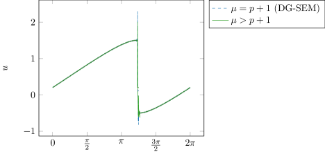
Figure 1. Comparison of $\mu=p+1$ (DG-SEM) with $\mu>p+1$ for Burgers’ equation, at $t=1.5$. Cell averages are indicated with plot markers.

Table 2. $L^{\infty}$ error and convergence rates for the smooth solution to 1D Burgers’ equation at $t=0.5$.

		$\mu=p+1$		$\mu>p+1$
	$N$	Error	Rate	Error	Rate
$p=2$	40	$3.27\times 10^{-3}$	—	$7.59\times 10^{-4}$	—
	80	$7.92\times 10^{-4}$	2.04	$1.06\times 10^{-4}$	2.84
	160	$2.08\times 10^{-4}$	1.93	$1.47\times 10^{-5}$	2.86
	320	$5.10\times 10^{-5}$	2.03	$1.93\times 10^{-6}$	2.93
$p=3$	40	$1.65\times 10^{-4}$	—	$3.84\times 10^{-5}$	—
	80	$1.62\times 10^{-5}$	3.35	$2.54\times 10^{-6}$	3.92
	160	$1.31\times 10^{-6}$	3.63	$1.80\times 10^{-7}$	3.82
	320	$9.34\times 10^{-8}$	3.81	$1.17\times 10^{-8}$	3.94
$p=4$	40	$1.13\times 10^{-5}$	—	$3.09\times 10^{-6}$	—
	80	$7.16\times 10^{-7}$	3.98	$1.08\times 10^{-7}$	4.85
	160	$4.34\times 10^{-8}$	4.04	$3.90\times 10^{-9}$	4.78
	320	$2.62\times 10^{-9}$	4.05	$1.29\times 10^{-10}$	4.92
$p=5$	40	$7.12\times 10^{-7}$	—	$1.64\times 10^{-7}$	—
	80	$1.87\times 10^{-8}$	5.25	$3.49\times 10^{-9}$	5.55
	160	$3.93\times 10^{-10}$	5.57	$6.07\times 10^{-11}$	5.85
	320	$1.32\times 10^{-11}$	4.89	$1.03\times 10^{-12}$	5.87

4.2. 1D shock tube

In this section, we consider both the classic shock tube problem of Sod, as well as a slightly modified Mach 2 shock tube problem. Both problems are solved on the domain $\Omega=[-0.5,0.5]$, and the initial conditions for both problems posses a discontinuity at the origin,

(78) $$\bm{u}_{0}(x)=\begin{cases}\bm{u}_{L},\qquad x<0,\\ \bm{u}_{R},\qquad x\geq 0.\end{cases}$$

The initial conditions for Sod’s shock tube are given by

(79) $$\bm{u}_{L}=\left(\begin{array}[]{c}\rho_{L}\\ w_{L}\\ p_{L}\end{array}\right)=\left(\begin{array}[]{c}1\\ 0\\ 1\end{array}\right),\qquad\bm{u}_{R}=\left(\begin{array}[]{c}\rho_{R}\\ w_{R}\\ p_{R}\end{array}\right)=\left(\begin{array}[]{c}1/8\\ 0\\ 1/10\end{array}\right).$$

The initial conditions for the Mach 2 shock are given by

(80) $$\bm{u}_{L}=\left(\begin{array}[]{c}\rho_{L}\\ w_{L}\\ p_{L}\end{array}\right)=\left(\begin{array}[]{c}1.162\\ 0\\ 4.5\end{array}\right),\qquad\bm{u}_{R}=\left(\begin{array}[]{c}\rho_{R}\\ w_{R}\\ p_{R}\end{array}\right)=\left(\begin{array}[]{c}1/8\\ 0\\ 1/10\end{array}\right).$$

Both problems give rise to a rarefaction wave, a contact discontinuity, and a shock. We solve both problems using $p=6$ polynomials with 48 elements, and integrate in time until $t=0.1$. A comparison of the numerical solutions with the exact solutions is shown in Figure 2. For the Sod shock tube problem, the DG-SEM method and Line-DG method with $\mu>p+1$ give comparable results. However, for the Mach 2 shock problem, the DG-SEM method gives rise to significantly more prominent oscillations, demonstrating a potential advantage of integrating with higher-accuracy quadrature rules. This phenomenon is particularly noticeable in the velocity component of the solution.

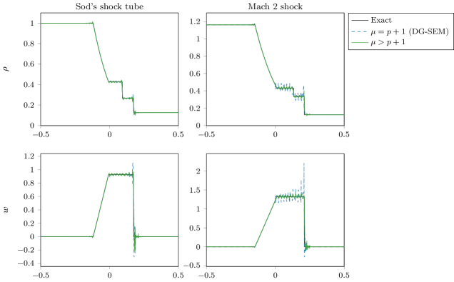
Figure 2. Numerical and exact solutions to the shock tube problems at $t=0.1$. Density is shown in the top row and velocity is shown in the bottom row.

4.3. 2D Burgers’ equation

For the first two-dimensional test problem, we consider the Line-DG method applied to the 2D Burgers’ equation,

(81) $$u_{t}+\nabla\cdot\left(\tfrac{1}{2}\bm{\beta}u^{2}\right)=0,$$

with constant velocity vector $\bm{\beta}=(1,1)$. We choose the smooth initial conditions $u_{0}(x,y)=\frac{1}{2}+\sin(x)\cos(y)$, and integrate in time until $t=0.5$. At this point, the solution remains smooth, and as in the 1D case, we can obtain the exact solution by tracing backwards along characteristic lines.

We compare the $L^{2}$ error obtained using the Line-DG method and the DG-SEM ($\mu=p+1$) method. We also consider the Line-DG method without the final quadrature projection. Results are shown in Table 3. For both the DG-SEM and Line-DG methods, we observe slightly sub-optimal convergence: approximately $\mathcal{O}(h^{p+1/2})$. Without the quadrature projection operation, the convergence is approximately $\mathcal{O}(h^{p+1})$, in accordance with Propositions 2 and 3. For each test case, the error obtained using the Line-DG method is smaller by approximately a factor of two, and the rate of convergence appears to be slightly faster than that of DG-SEM for a majority of cases. We also investigate the entropy dissipation of each of these methods. Since both methods are entropy-stable, the total entropy must be monotonically non-increasing. For this test case the solution is smooth, and so the entropy for the exact solution remains constant. In Figure 3, we compare the relative deviation from the initial entropy, measured by $\int_{\Omega}\left(U(\bm{x},t)-U(\bm{x},0)\right)\,d\bm{x}/\int_{\Omega}U(\bm{x},0)\,d\bm{x}$, where $U(x,t)$ is the square entropy, $U(x,t)=\frac{1}{2}u(x,t)^{2}$. We numerically observe the entropy stability of both methods, but note that the Line-DG method dissipates less entropy than the DG-SEM method.

Table 3. $L^{2}$ error and convergence rates for the smooth solution to 2D Burgers’ equation at $t=0.5$.

		$\mu=p+1$		$\mu>p+1$		No projection
	$N$	Error	Rate	Error	Rate	Error	Rate
$p=2$	12	$4.03\times 10^{-2}$	—	$2.65\times 10^{-2}$	—	$2.20\times 10^{-3}$	—
	24	$9.20\times 10^{-3}$	2.13	$4.11\times 10^{-3}$	2.69	$2.20\times 10^{-3}$	2.90
	48	$1.83\times 10^{-3}$	2.33	$6.72\times 10^{-4}$	2.61	$3.06\times 10^{-4}$	2.84
	96	$3.43\times 10^{-4}$	2.41	$1.11\times 10^{-4}$	2.60	$4.21\times 10^{-5}$	2.86
$p=3$	12	$8.03\times 10^{-3}$	—	$3.54\times 10^{-3}$	—	$2.46\times 10^{-3}$	—
	24	$8.01\times 10^{-4}$	3.32	$3.73\times 10^{-4}$	3.25	$2.08\times 10^{-4}$	3.57
	48	$7.66\times 10^{-5}$	3.39	$3.47\times 10^{-5}$	3.43	$1.54\times 10^{-5}$	3.76
	96	$6.67\times 10^{-6}$	3.52	$3.14\times 10^{-6}$	3.47	$1.08\times 10^{-6}$	3.83
$p=4$	12	$1.37\times 10^{-3}$	—	$8.02\times 10^{-4}$	—	$6.40\times 10^{-4}$	—
	24	$9.46\times 10^{-5}$	3.85	$3.67\times 10^{-5}$	4.45	$2.51\times 10^{-5}$	4.67
	48	$4.84\times 10^{-6}$	4.29	$1.60\times 10^{-6}$	4.52	$9.60\times 10^{-7}$	4.71
	96	$2.27\times 10^{-7}$	4.42	$7.05\times 10^{-8}$	4.50	$3.43\times 10^{-8}$	4.81
$p=5$	12	$3.78\times 10^{-4}$	—	$1.86\times 10^{-4}$	—	$1.54\times 10^{-4}$	—
	24	$1.19\times 10^{-5}$	4.99	$4.90\times 10^{-6}$	5.25	$3.52\times 10^{-6}$	5.45
	48	$3.15\times 10^{-7}$	5.24	$1.08\times 10^{-7}$	5.50	$6.77\times 10^{-8}$	5.70
	96	$7.06\times 10^{-9}$	5.48	$2.35\times 10^{-9}$	5.53	$1.23\times 10^{-9}$	5.79

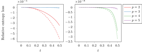
Figure 3. Relative entropy loss for the 2D Burgers’ equation, with $U=\frac{1}{2}u^{2}$, for $N=12$ and $p=2,3,4,5$. Line-DG shown with solid lines, DG-SEM shown with dashed lines.

As a final investigation into the entropy conservation and stability properties of the method, we consider using the entropy conservative numerical flux function at element interfaces by defining, as in [12],

(82) $$\widehat{\bm{f}_{S}}(u_{L},u_{R})\cdot\bm{n}=\frac{1}{6}\left(u_{L}^{2}+u_{L}u_{R}+u_{R}^{2}\right)\bm{\beta}\cdot\bm{n}.$$

This is not a physically relevant choice of numerical flux function for Burgers’ equation because it fails to dissipate entropy across discontinuities. However, it is useful to test the numerical properties of the scheme. We now solve the same problem as above, but integrate in time until $t=1.25$, at which point the solution has developed discontinuities, and thus the entropy of the true solution is less than the entropy of the initial condition. In Figure 4 we compare the relative entropy loss of the Line-DG method using both (entropy stable) exact Riemann solver and the entropy conservative numerical flux function (82) at element interfaces. These results confirm that using the entropy conservative numerical flux function gives unchanged entropy (to machine precision) throughout the duration of the simulation, numerically confirming the results shown in Proposition 5.

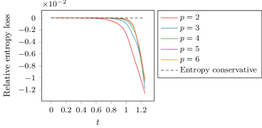
Figure 4. Relative entropy loss for the 2D Burgers’ equation at $t=1.25$, for $N=12$ and $p=2,3,4,5,6$ using the Line-DG method. Results obtained using the exact Riemann solver are shown in solid lines, results using the entropy conservative flux are shown in dashed lines.

4.4. 2D isentropic vortex

For this test problem, we study the accuracy of the Line-DG method applied to the isentropic Euler vortex test case [42]. This problem consists of an isentropic vortex that is advected with the freestream velocity, and is often used as a smooth benchmark problem [26, 44]. The spatial domain is taken to be $[0,20]\times[0,15]$. The vortex is initially centered at $(x_{0},y_{0})=(5,5)$, and is advected at an angle of $\theta$. The exact solution at position and time $(x,y,t)$ is given by

(83) $$\rho(x,y,t) =\rho_{\infty}\left(1-\frac{\epsilon^{2}(\gamma-1)M^{2}_{\infty}}{8\pi^{2}}\exp(f(x,y,t))\right)^{\frac{1}{\gamma-1}},$$

$$w_{1}(x,y,t) =w_{\infty}\left(\cos(\theta)-\frac{\epsilon((y-y_{0})-\overline{w_{2}}t)}{2\pi r_{c}}\exp\left(\frac{f(x,y,t)}{2}\right)\right),$$

$$w_{2}(x,y,t) =w_{\infty}\left(\sin(\theta)-\frac{\epsilon((x-x_{0})-\overline{w_{1}}t)}{2\pi r_{c}}\exp\left(\frac{f(x,y,t)}{2}\right)\right),$$

$$p(x,y,t) =p_{\infty}\left(1-\frac{\epsilon^{2}(\gamma-1)M^{2}_{\infty}}{8\pi^{2}}\exp(f(x,y,t))\right)^{\frac{\gamma}{\gamma-1}},$$

where $f(x,y,t)=(1-((x-x_{0})-\overline{w_{1}}t)^{2}-((y-y_{0})-\overline{w_{2}}t)^{2})/r_{c}^{2}$, $M_{\infty}$ is the freestream Mach number, and $w_{\infty},\rho_{\infty},$ and $p_{\infty}$ are the freestream velocity magnitude, density, and pressure, respectively. The freestream velocity is given by $(\overline{w_{1}},\overline{w_{2}})=w_{\infty}(\cos(\theta),\sin(\theta))$. The strength of the vortex is given by $\epsilon$, and its size by $r_{c}$. We choose the parameters to be $M_{\infty}=0.5$, $w_{\infty}=1$, $\theta=\arctan(1/2)$, $\epsilon=5/(2\pi)$, and $r_{c}=1.5$. We integrate the equations until $t=5$.

We perform a convergence study to investigate the effects of the projection operation described in Section 2.4.1 on the accuracy of the method. Additionally, for comparison we consider a fully-integrated standard DG method. The local Lax-Friedrichs numerical flux function was used for all methods. The $L^{\infty}$ error at the final time is shown in Figure 5. We observe that the Line-DG method without the projection operation has accuracy that is almost identical to that of the standard, fully-integrated DG method for this test problem. This finding is consistent with the results shown in [29]. However, when the projection operation is performed in order to ensure discrete entropy stability, we observe a larger error by approximately a constant factor. It is interesting to note that for this test problem, we do not observe the sub-optimal order of accuracy seen in previous test cases. This is possibly due to the translational nature of the true solution.

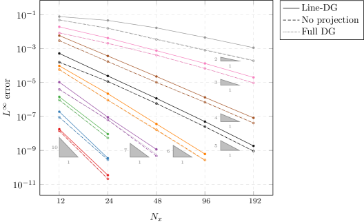
Figure 5. $L^{\infty}$ error for isentropic Euler vortex problem with polynomial degrees $p=1,2,\ldots,9$. Optimal order of accuracy is observed for all cases. Solid lines indicate the entropy-stable Line-DG method. Dashed lines indicate Line-DG without the projection operation. Dotted lines indicate fully-integrated standard DG.

4.5. 2D supersonic flow in a duct

We consider the inviscid supersonic flow in a duct with a smooth bump. The duct has dimensions $3\times 1$ and the $y$-coordinate of the bottom boundary is given by

(84) $$y(x)=\begin{cases}\frac{H}{2}\left(\cos(\pi(1+2(x-3/4))+1\right),&\qquad 3/4<x<5/4\\ H,&\qquad 5/4\leq x\leq 7/4\\ \frac{H}{2}\left(\cos(2\pi(x-7/4))+1\right),&\qquad 7/4<x<9/4\\ 0,&\qquad\text{otherwise.}\end{cases}$$

where the height of the bump is given by $H=0.04$. The inflow density is $\rho=1$, and the inflow velocity is $\bm{w}=(1,0)$. We set the Mach number to $M=1.4$ as in [10]. Slip wall conditions are enforced on the top and bottom boundaries. The curved boundary is represented using isoparametric elements. We use 675 elements with degree $p=4$ polynomials. We do not use any shock capturing techniques or apply any limiters to the solution. This test case is intended to assess the robustness of the method for under-resolved high Mach number flow.

We compute the steady solution to this problem using pseudo-time integration. We compare the solutions obtained using the $\mu=p+1$ DG-SEM method to the Line-DG method with $\mu>p+1$. The steady-state pressure is shown in Figure 6. Both solutions display fairly severe oscillations in the vicinity of the shocks. Some of these features appear to be more prominent in the solution obtained using the DG-SEM method. Despite these oscillations, the method remains robust due to the entropy stability. Traditional DG-SEM, Line-DG, or consistently-integrated standard DG methods are unstable for this problem without the use of additional shock capturing techniques or limiters.

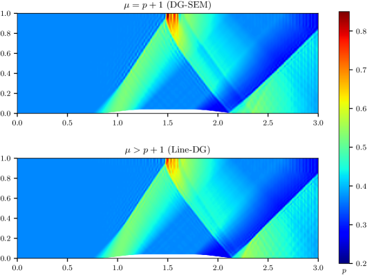
Figure 6. Density of steady-state solution to supersonic flow over a bump.

We also use this test to verify the freestream preservation of the method, which is widely known to be an important property [40]. We initialize the solution to uniform flow and enforce freestream boundary conditions at all boundaries. We then integrate in time and monitor the deviation of the solution from the initial freestream conditions. We use $p=2$ polynomials and consider both the Line-DG and DG-SEM methods, and integrate until a final time of $t=1$. Both methods resulted in only machine precision deviation from freestream conditions. The $L^{\infty}$ deviation from the freestream density was found to be about $4.4\times 10^{-14}$ using the DG-SEM method and about $4.9\times 10^{-14}$ using the Line-DG method.

4.6. 3D inviscid Taylor-Green vortex

For a final set of test cases, we consider the compressible, inviscid Taylor-Green vortex (TGV) [39] at different Mach numbers. This problem has been extensively studied for the incompressible case [2], as well as the nearly-incompressible case [35, 6, 25, 27]. The stability of DG discretizations for the under-resolved simulation of the inviscid TGV has also been studied in [43, 21]. The domain is taken to be the cube $[-\pi,\pi]^{3}$, and periodic conditions are enforced on all boundaries. The initial conditions are given by

(85) $$\rho(x,y,z) =\rho_{0}$$

$$w_{1}(x,y,z) =w_{0}\sin(x)\cos(y)\cos(z)$$

$$w_{2}(x,y,z) =-w_{0}\cos(x)\sin(y)\cos(z)$$

$$w_{3}(x,y,z) =0$$

$$p(x,y,z) =p_{0}+\rho_{0}u_{0}^{2}\left(\cos(2x)+\cos(2y)\right)\left(\cos(2z)+2\right)/16,$$

where we take the parameters to be $w_{0}=1$, $\rho_{0}=1$, with Mach number $M_{0}=u_{0}/c_{0}$, where $c_{0}$ is the speed of sound computed in accordance with the pressure $p_{0}$. The characteristic convective time is given by $t_{\rm c}=1$, and we integrate until $t=10t_{\rm c}$. For the nearly incompressible case, we choose $p_{0}=100$ which corresponds to a Mach number of $M_{0}\approx 0.08$. We also consider a higher Mach number case defined by $M_{0}=0.7$.

We measure three quantities of interest. The first is the mean entropy, which is guaranteed to be monotonically non-increasing by the method. The second is the mean kinetic energy

(86) $$E_{k}(t)=\frac{1}{\rho_{0}|\Omega|}\int_{\Omega}\tfrac{1}{2}\rho\bm{w}\cdot\bm{w}\,d\bm{x}.$$

We can easily see that $E_{k}(0)=1/8$. Since the kinetic energy is conserved for the inviscid Taylor-Green vortex in the incompressible limit, for the low Mach (nearly incompressible) case, we can use $E_{k}(t)$ as a measure of the numerical dissipation introduced by the discretization. The third quantity of interest considered is the mean enstrophy, defined by

(87) $$\mathcal{E}(t)=\frac{1}{\rho_{0}|\Omega|}\int_{\Omega}\tfrac{1}{2}\rho\bm{\omega}\cdot\bm{\omega}\,d\bm{x},$$

where $\bm{\omega}=\nabla\times\bm{w}$ is the vorticity. The enstrophy can be used as a measure of the resolving power of the numerical discretization [35]. These integrals are discretized using a consistent quadrature with $\mu$ points in each dimension.

We discretize the geometry using a $20\times 20\times 20$ Cartesian grid, and we use degree $p=3$ and $p=5$ polynomials. For the higher Mach number case, defined by $M=0.7$, the standard DG-SEM method without entropy stability is unstable after about $t=3.9t_{\rm c}$. The Line-DG method without entropy stability is unstable after about $t=4.7t_{\rm c}$. The entropy-stable versions of both DG-SEM and Line-DG remain stable for the full duration of the simulation. These stability issues were not observed for the nearly incompressible case.

In Figure 7, we show the normalized time evolution of the quantities of interest for both test cases. We define the normalized mean entropy by $\int_{\Omega}\left(U(\bm{x},t)-U(\bm{x},0)\right)\,d\bm{x}/\int_{\Omega}U(\bm{x},0)\,d\bm{x}$, and similarly for the normalized mean kinetic energy and enstrophy. For the low Mach case with $p=3$ polynomials, we notice that the Line-DG method dissipates less entropy and kinetic energy than the equal-order DG-SEM method. In fact, the dissipation of these two quantities is roughly equivalent to the DG-SEM method with polynomial degree $p=5$. For both the Line-DG method and DG-SEM method with $p=3$, the peak enstrophy is under-predicted. For the $M_{0}=0.7$ case, the Line-DG and DG-SEM methods result in comparable results for all three quantities considered, however for the $p=5$ case, the DG-SEM method gives rise to less enstrophy growth. As discussed in [35], some caution is required when using these mean quantities to assess the quality of the numerical solutions, in particular once the solution has become under-resolved.

This test case demonstrates both the increased robustness of the entropy-stable Line-DG when compared with standard DG methods, and its low dissipation when compared with the equal-order entropy-stable DG-SEM method.

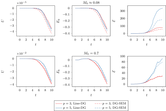
Figure 7. Normalized time evolution of $U$ (entropy), $E_{k}$ (kinetic energy), and $\mathcal{E}$ (enstrophy) over time, for the 3D inviscid Taylor-Green test case, at $M_{0}\approx 0.08$ and $M_{0}=0.7$.

5. Conclusions

In this paper, we have constructed a discretely entropy-stable line-based discontinuous Galerkin method. We modify the Line-DG method of [28, 29] using a flux differencing technique in order to obtain discrete entropy stability, compatible with the quadrature rule used in the discretization. This line-based method is composed of one-dimensional operations performed along lines or curves of nodes within tensor-product elements, resulting in fewer flux evaluations, and requiring only one-dimensional interpolation and integration operations. This method is closely related to the entropy-stable DG-SEM method, described in [7, 3, 11], and to the entropy-stable full DG method developed in [4]. When compared with the equal-order entropy-stable DG-SEM method on a range of test cases, the Line-DG method results in smaller errors and less numerical dissipation.

The main feature of this entropy-stable method is its increased robustness in the presence of shocks or under-resolved features. This robustness has been demonstrated on a range of problems for which standard DG-type methods are unstable without the use of additional limiting or shock-capturing techniques. For problems with strong shocks, the entropy-stable Line-DG method can demonstrate spurious oscillations despite remaining stable. For problems of this type, artificial viscosity or limiters may be used to reduce the oscillations and increase solution quality.

6. Acknowledgements

This work was supported by the National Aeronautics and Space Administration (NASA) under grant number NNX16AP15A, by the Director, Office of Science, Office of Advanced Scientific Computing Research, U.S. Department of Energy under Contract No. DE-AC02-05CH11231 and by the AFOSR Computational Mathematics program under grant number FA9550-15-1-0010. Lawrence Livermore National Laboratory is operated by Lawrence Livermore National Security, LLC, for the U.S. Department of Energy, National Nuclear Security Administration under Contract DE-AC52-07NA27344 (LLNL-JRNL-767379).

References

- [1] Black, K.: Spectral element approximation of convection-diffusion type problems. Applied Numerical Mathematics 33(1-4), 373–379 (2000). DOI 10.1016/s0168-9274(99)00104-x
- [2] Brachet, M.E., Meiron, D.I., Orszag, S.A., Nickel, B.G., Morf, R.H., Frisch, U.: Small-scale structure of the Taylor-Green vortex. Journal of Fluid Mechanics 130(-1), 411 (1983). DOI 10.1017/s0022112083001159
- [3] Carpenter, M.H., Fisher, T.C., Nielsen, E.J., Frankel, S.H.: Entropy stable spectral collocation schemes for the Navier-Stokes equations: discontinuous interfaces. SIAM Journal on Scientific Computing 36(5), B835–B867 (2014). DOI 10.1137/130932193
- [4] Chan, J.: On discretely entropy conservative and entropy stable discontinuous Galerkin methods. Journal of Computational Physics 362, 346–374 (2018). DOI 10.1016/j.jcp.2018.02.033
- [5] Chandrashekar, P.: Kinetic energy preserving and entropy stable finite volume schemes for compressible Euler and Navier-Stokes equations. Communications in Computational Physics 14(05), 1252–1286 (2013). DOI 10.4208/cicp.170712.010313a
- [6] Chapelier, J.B., Plata, M.D.L.L., Renac, F.: Inviscid and viscous simulations of the Taylor-green vortex flow using a modal discontinuous Galerkin approach. In: 42nd AIAA Fluid Dynamics Conference and Exhibit. American Institute of Aeronautics and Astronautics (2012). DOI 10.2514/6.2012-3073
- [7] Chen, T., Shu, C.W.: Entropy stable high order discontinuous Galerkin methods with suitable quadrature rules for hyperbolic conservation laws. Journal of Computational Physics 345, 427–461 (2017). DOI 10.1016/j.jcp.2017.05.025
- [8] Cockburn, B., Shu, C.W.: The Runge-Kutta local projection -discontinuous-Galerkin finite element method for scalar conservation laws. ESAIM: Mathematical Modelling and Numerical Analysis 25(3), 337–361 (1991). DOI 10.1051/m2an/1991250303371
- [9] Cockburn, B., Shu, C.W.: Runge-Kutta discontinuous Galerkin methods for convection-dominated problems. Journal of Scientific Computing 16(3), 173–261 (2001). DOI 10.1023/A:1012873910884
- [10] Fernandez, P., Nguyen, N.C., Peraire, J.: Entropy-stable hybridized discontinuous Galerkin methods for the compressible Euler and Navier-Stokes equations (2018). ArXiv:1808.05066
- [11] Fisher, T.C., Carpenter, M.H.: High-order entropy stable finite difference schemes for nonlinear conservation laws: Finite domains. Journal of Computational Physics 252, 518–557 (2013). DOI 10.1016/j.jcp.2013.06.014
- [12] Gassner, G.J.: A skew-symmetric discontinuous Galerkin spectral element discretization and its relation to SBP-SAT finite difference methods. SIAM Journal on Scientific Computing 35(3), A1233–A1253 (2013). DOI 10.1137/120890144
- [13] Gassner, G.J., Winters, A.R., Kopriva, D.A.: Split form nodal discontinuous Galerkin schemes with summation-by-parts property for the compressible Euler equations. Journal of Computational Physics 327, 39–66 (2016). DOI 10.1016/j.jcp.2016.09.013
- [14] Harten, A.: On the symmetric form of systems of conservation laws with entropy. Journal of Computational Physics 49(1), 151–164 (1983). DOI 10.1016/0021-9991(83)90118-3
- [15] Hou, S., Liu, X.D.: Solutions of multi-dimensional hyperbolic systems of conservation laws by square entropy condition satisfying discontinuous Galerkin method. Journal of Scientific Computing 31(1-2), 127–151 (2006). DOI 10.1007/s10915-006-9105-9
- [16] Hughes, T., Franca, L., Mallet, M.: A new finite element formulation for computational fluid dynamics: I. Symmetric forms of the compressible Euler and Navier-Stokes equations and the second law of thermodynamics. Computer Methods in Applied Mechanics and Engineering 54(2), 223–234 (1986). DOI 10.1016/0045-7825(86)90127-1
- [17] Ismail, F., Roe, P.L.: Affordable, entropy-consistent Euler flux functions II: Entropy production at shocks. Journal of Computational Physics 228(15), 5410–5436 (2009). DOI 10.1016/j.jcp.2009.04.021
- [18] Jiang, G., Shu, C.W.: On a cell entropy inequality for discontinuous Galerkin methods. Mathematics of Computation 62(206), 531 (1994). DOI 10.2307/2153521
- [19] Kopriva, D.A.: Metric identities and the discontinuous spectral element method on curvilinear meshes. Journal of Scientific Computing 26(3), 301–327 (2006). DOI 10.1007/s10915-005-9070-8
- [20] Kopriva, D.A., Kolias, J.H.: A conservative staggered-grid Chebyshev multidomain method for compressible flows. Journal of Computational Physics 125(1), 244–261 (1996). DOI 10.1006/jcph.1996.0091
- [21] Moura, R., Mengaldo, G., Peiró, J., Sherwin, S.: On the eddy-resolving capability of high-order discontinuous Galerkin approaches to implicit LES / under-resolved DNS of Euler turbulence. Journal of Computational Physics 330, 615–623 (2017). DOI 10.1016/j.jcp.2016.10.056
- [22] Orszag, S.A.: Spectral methods for problems in complex geometries. Journal of Computational Physics 37(1), 70 – 92 (1980). DOI 10.1016/0021-9991(80)90005-4
- [23] Osher, S., Tadmor, E.: On the convergence of difference approximations to scalar conservation laws. Mathematics of Computation 50(181), 19–19 (1988). DOI 10.1090/s0025-5718-1988-0917817-x
- [24] Parsani, M., Carpenter, M.H., Fisher, T.C., Nielsen, E.J.: Entropy stable staggered grid discontinuous spectral collocation methods of any order for the compressible Navier–Stokes equations. SIAM Journal on Scientific Computing 38(5), A3129–A3162 (2016). DOI 10.1137/15m1043510
- [25] Pazner, W., Persson, P.O.: High-order DNS and LES simulations using an implicit tensor-product discontinuous Galerkin method. In: 23rd AIAA Computational Fluid Dynamics Conference. American Institute of Aeronautics and Astronautics (2017). DOI 10.2514/6.2017-3948
- [26] Pazner, W., Persson, P.O.: Stage-parallel fully implicit Runge-Kutta solvers for discontinuous Galerkin fluid simulations. Journal of Computational Physics 335, 700–717 (2017). DOI 10.1016/j.jcp.2017.01.050
- [27] Pazner, W., Persson, P.O.: Approximate tensor-product preconditioners for very high order discontinuous Galerkin methods. Journal of Computational Physics 354, 344–369 (2018). DOI 10.1016/j.jcp.2017.10.030
- [28] Persson, P.O.: High-order Navier-Stokes simulations using a sparse line-based discontinuous Galerkin method. In: 50th AIAA Aerospace Sciences Meeting including the New Horizons Forum and Aerospace Exposition. American Institute of Aeronautics and Astronautics (2012). DOI 10.2514/6.2012-456
- [29] Persson, P.O.: A sparse and high-order accurate line-based discontinuous Galerkin method for unstructured meshes. Journal of Computational Physics 233, 414–429 (2013). DOI 10.1016/j.jcp.2012.09.008
- [30] Persson, P.O., Peraire, J.: Sub-cell shock capturing for discontinuous Galerkin methods. In: 44th AIAA Aerospace Sciences Meeting and Exhibit. American Institute of Aeronautics and Astronautics (2006). DOI 10.2514/6.2006-112
- [31] Ranocha, H.: Comparison of some entropy conservative numerical fluxes for the Euler equations. Journal of Scientific Computing 76(1), 216–242 (2017). DOI 10.1007/s10915-017-0618-1
- [32] Rasetarinera, P., Hussaini, M.: An efficient implicit discontinuous spectral Galerkin method. Journal of Computational Physics 172(2), 718–738 (2001). DOI 10.1006/jcph.2001.6853
- [33] Ray, D., Chandrashekar, P.: Entropy stable schemes for compressible Euler equations. International Journal of Numerical Analysis and Modeling, Series B 4(4), 335–352 (2013)
- [34] Reed, W.H., Hill, T.R.: Triangular mesh methods for the neutron transport equation. Los Alamos Report LA-UR-73-479 (1973)
- [35] Shu, C.W., Don, W.S., Gottlieb, D., Schilling, O., Jameson, L.: Numerical convergence study of nearly incompressible, inviscid Taylor-Green vortex flow. Journal of Scientific Computing 24(1), 1–27 (2005). DOI 10.1007/s10915-004-5407-y
- [36] Sørensen, H.H.B.: Auto-tuning of level 1 and level 2 BLAS for GPUs. Concurrency and Computation: Practice and Experience 25(8), 1183–1198 (2012). DOI 10.1002/cpe.2916
- [37] Tadmor, E.: Entropy stability theory for difference approximations of nonlinear conservation laws and related time-dependent problems. In: A. Iserles (ed.) Acta Numerica 2003, pp. 451–512. Cambridge University Press. DOI 10.1017/cbo9780511550157.007
- [38] Tadmor, E.: The numerical viscosity of entropy stable schemes for systems of conservation laws. I. Mathematics of Computation 49(179), 91–91 (1987). DOI 10.1090/s0025-5718-1987-0890255-3
- [39] Taylor, G.I., Green, A.E.: Mechanism of the production of small eddies from large ones. Proceedings of the Royal Society A: Mathematical, Physical and Engineering Sciences 158(895), 499–521 (1937). DOI 10.1098/rspa.1937.0036
- [40] Thomas, P.D., Lombard, C.K.: Geometric conservation law and its application to flow computations on moving grids. AIAA Journal 17(10), 1030–1037 (1979). DOI 10.2514/3.61273
- [41] Vos, P.E., Sherwin, S.J., Kirby, R.M.: From to efficiently: implementing finite and spectral/ element methods to achieve optimal performance for low- and high-order discretisations. Journal of Computational Physics 229(13), 5161–5181 (2010). DOI 10.1016/j.jcp.2010.03.031
- [42] Wang, Z., Fidkowski, K., Abgrall, R., Bassi, F., Caraeni, D., Cary, A., Deconinck, H., Hartmann, R., Hillewaert, K., Huynh, H., Kroll, N., May, G., Persson, P.O., van Leer, B., Visbal, M.: High-order CFD methods: current status and perspective. International Journal for Numerical Methods in Fluids 72(8), 811–845 (2013). DOI 10.1002/fld.3767
- [43] Winters, A.R., Moura, R.C., Mengaldo, G., Gassner, G.J., Walch, S., Peiro, J., Sherwin, S.J.: A comparative study on polynomial dealiasing and split form discontinuous Galerkin schemes for under-resolved turbulence computations. Journal of Computational Physics 372, 1–21 (2018). DOI 10.1016/j.jcp.2018.06.016
- [44] Zahr, M.J., Persson, P.O.: Performance tuning of Newton-GMRES methods for discontinuous Galerkin discretizations of the Navier-Stokes equations. In: 21st AIAA Computational Fluid Dynamics Conference. American Institute of Aeronautics and Astronautics (2013). DOI 10.2514/6.2013-2685
- [45] Zhang, X., Shu, C.W.: On positivity-preserving high order discontinuous Galerkin schemes for compressible Euler equations on rectangular meshes. Journal of Computational Physics 229(23), 8918–8934 (2010). DOI 10.1016/j.jcp.2010.08.016
- [46] Zingan, V., Guermond, J.L., Morel, J., Popov, B.: Implementation of the entropy viscosity method with the discontinuous Galerkin method. Computer Methods in Applied Mechanics and Engineering 253, 479–490 (2013). DOI 10.1016/j.cma.2012.08.018