Periodic solutions and torsional instability
in a nonlinear nonlocal plate equation

Abstract.

A thin and narrow rectangular plate having the two short edges hinged and the two long edges free is considered. A nonlinear nonlocal evolution equation describing the deformation of the plate is introduced: well-posedness and existence of periodic solutions are proved. The natural phase space is a particular second order Sobolev space that can be orthogonally split into two subspaces containing, respectively, the longitudinal and the torsional movements of the plate. Sufficient conditions for the stability of periodic solutions and of solutions having only a longitudinal component are given. A stability analysis of the so-called prevailing mode is also performed. Some numerical experiments show that instabilities may occur. This plate can be seen as a simplified and qualitative model for the deck of a suspension bridge, which does not take into account the complex interactions between all the components of a real bridge.

To Cecília

1. Introduction

We consider a thin and narrow rectangular plate with the two short edges hinged while the two long edges are free. In absence of forces, the plate lies horizontally flat and is represented by the planar domain $\Omega=(0,\pi)\times(-\ell,\ell)$ with $0<\ell\ll\pi$. The plate is subject both to dead and live loads acting orthogonally on $\Omega$ and to compressive forces along the edges, the so-called buckling loads. We follow the plate model suggested by Berger [8]; see also the former beam model by Woinowsky-Krieger [40] and, independently, by Burgreen [11]. Then the nonlocal evolution equation modeling the deformation of the plate reads

(5) $$\left\{\begin{array}[]{rl}u_{tt}+\delta u_{t}+\Delta^{2}u+\left[P-S\int_{\Omega}u_{x}^{2}\right]u_{xx}=g&\textrm{in }\Omega\times(0,T)\\ u=u_{xx}=0&\textrm{on }\{0,\pi\}\times[-\ell,\ell]\\ u_{yy}+\sigma u_{xx}=u_{yyy}+(2-\sigma)u_{xxy}=0&\textrm{on }[0,\pi]\times\{-\ell,\ell\}\\ u(x,y,0)=u_{0}(x,y),\quad\quad u_{t}(x,y,0)=v_{0}(x,y)&\textrm{in }\Omega\,.\end{array}\right.$$

All the parameters in (5) and their physical meaning will be discussed in detail in Section 2. The plate $\Omega$ can be seen as a simplified model for the deck of a suspension bridge. Even if the model does not take into account the complex interactions between all the components of a real bridge, we expect to observe the phenomena seen on built bridges. Therefore we will often refer to the scenario described in the engineering literature and tackle the stability issue only qualitatively.

A crucial role in the collapse of several bridges is played by the mode of oscillation. In particular, as shown in the video [36], the “two waves” were torsional oscillations and were considered the main cause of the Tacoma Narrows Bridge (TNB) collapse [3, 32]. The very same oscillations also caused several other bridges collapses: among others, we mention the Brighton Chain Pier in 1836, the Menai Straits Bridge in 1839, the Wheeling Suspension Bridge in 1854, the Matukituki Suspension Footbridge in 1977; see [19, Chapter 1] for a detailed description of these collapses. The distinguished civil and aeronautical engineer Robert Scanlan [31, p.209] attributed the appearance of torsional oscillations at the TNB to some fortuitous condition: the word “fortuitous” denotes a lack of rigorous explanations and, according to [32], no fully satisfactory explanation has been reached in subsequent years. In fact, no purely aerodynamic explanation was able to justify the origin of the torsional oscillation, which is the main culprit for the collapse of the TNB. More recently [4, 7], for slightly different bridge models, the attention was put on the nonlinear structural behavior of suspension bridges: the bridge was considered isolated from aerodynamic effects and dissipation. The results therein show that the origin of torsional instability is structural and explain why the TNB withstood larger longitudinal oscillations on low modes, but failed for smaller longitudinal oscillations on higher modes, see [3, pp.28-31]. It is shown in [4, 7] that if the longitudinal oscillation is sufficiently large, then a structural instability appears and this is the onset of torsional oscillations. In these papers, the main focus was on the structural behavior and the action of the wind was missing.

From the Report [3, pp.118-120] we learn that for the recorded oscillations at the TNB one definite mode of oscillation prevailed over a certain interval of time. However, the modes frequently changed. The suggested target was to find a possible correlation between the wind velocity and the prevailing mode and the conclusion was that a definite correlation exists between frequencies and wind velocities: higher velocities favor modes with higher frequencies. On the other hand, just a few days prior to the TNB collapse, the project engineer L.R. Durkee wrote a letter (see [3, p.28]) describing the oscillations which were so far observed at the TNB. He wrote: Altogether, seven different motions have been definitely identified on the main span of the bridge, and likewise duplicated on the model. These different wave actions consist of motions from the simplest, that of no nodes, to the most complex, that of seven nodes. According to Eldridge [3, V-3], a witness on the day of the TNB collapse, the bridge appeared to be behaving in the customary manner and the motions were considerably less than had occurred many times before. Moreover, also Farquharson [3, V-10] witnessed the collapse and wrote that the motions, which a moment before had involved a number of waves (nine or ten) had shifted almost instantly to two.

Aiming to explain and possibly reproduce these phenomena, we proceed as follows. Firstly, we introduce in (5) the aerodynamic and dissipative effects, thereby completing the isolated models in [4, 7]. Then we try to give answers to the questions left open by the above discussion:

1. What is the correlation between the wind velocity and the prevailing mode of oscillation?

2. How stable is the prevailing longitudinal mode with respect to torsional perturbations?

To this end, the first step is to go through fine properties of the vibrating modes, both by estimating their frequencies (eigenvalues of a suitable problem) and by classifying them into longitudinal and torsional. This is done in Section 3 where we also decompose the phase space of (5) as direct sum of the orthogonal subspaces of longitudinal functions and of torsional functions. Theorems 5 and 6 show that (5) is well-posed and that the equation admits periodic solutions whenever the source $g$ is itself periodic. These solutions play an important role in our stability analysis which is characterized in Definition 7: roughly speaking, we say that (5) is torsionally stable if the torsional part of any solution tends to vanish at infinity and torsionally unstable otherwise, see also Proposition 8. In Theorem 9 we establish that if the forcing term $g$ is sufficiently small, then (5) has a “squeezing property” as in [20, (2.7)], namely all its solutions have the same behavior as $t\to\infty$. This enables us to prove both the uniqueness of a periodic solution (if $g$ is periodic) and to obtain a sufficient condition for the torsional stability (if $g$ is even with respect to $y$). By exploiting an argument by Souplet [34], in Theorem 10 we show that this smallness condition is “almost necessary” since multiple periodic solutions may exist in general. Theorem 11 states a similar property, but more related to applications: we obtain torsional stability for any given force $g$, provided that the damping coefficient $\delta$ is sufficiently large. Finally, in Theorem 12 we show that the responsible for possible instabilities is the nonlinear nonlocal term $\|u_{x}\|_{L^{2}}^{2}u_{xx}$ which acts a coupling term and allows transfer of energy between longitudinal and torsional oscillations.

Our results are complemented with some numerics aiming to describe the behavior of the solutions of (5) and to discuss the just mentioned sufficient conditions for the torsional stability. Overall, the numerical results, combined with our theorems, allow to answer to question (b): the stability of the prevailing longitudinal mode depends on its amplitude of oscillation, on its frequency of oscillation, and on the torsional mode that perturbs the motion. In order to answer to question (a), in Section 5 we perform a linear analysis. Our conclusion is that the prevailing mode is determined by the frequency of the forcing term $g$: there exist ranges of frequencies for $g$, each one of them exciting a particular longitudinal mode which then plays the role of the prevailing mode.

This paper is organized as follows. In order to have physically meaningful results, in Section 2 we describe in detail the model and the physical meaning of all the parameters in (5). In Section 3 we recall and improve some results about the spectrum of the linear elliptic operator in (5). In Section 4 we state our main results. These results are complemented with the linear analysis of Section 5, that enables us to answer to question (a), and with the numerical experiments reported in Section 6, that enable us to answer to question (b). Section 7 contains some energy bounds, useful for the proofs of our results that are contained in the remaining sections, from 8 to 13.

2. The physical model

In this section we perform space and time scalings that will reduce the dimensional equation

(6) $$M\,u_{tt}(\xi,t)+\varepsilon u_{t}(\xi,t)+D\,\Delta^{2}u(\xi,t)+\left[P-\frac{AE}{2L}\int_{\Omega}u_{x}^{2}(z,t)dz\right]u_{xx}(\xi,t)=g(\xi,t)\quad\mbox{in }\Omega\times(0,T)$$

to the slightly simpler form (5). Here and in the sequel, for simplicity we put

$$\xi:=(x,y)\in\Omega\,.$$

Let us explain the meaning of the structural constants appearing in (6):

$\Omega=(0,L)\times(-\ell,\ell)$ = the horizontal face of the rectangular plate

$L$ = length of the plate

$2\ell$ = width of the plate

$d$ = thickness of the plate

$H$ = frontal dimension (the height of the windward face of the plate)

$A=2\ell d$ = cross-sectional area of the plate

$\sigma$ = Poisson ratio of the material composing the plate

$D$ = flexural rigidity of the plate (the force couple required to bend it in one unit of curvature)

$M$ = surface density of mass of the plate

$P$ = prestressing constant (see [11])

$\varepsilon$ = damping coefficient

If the plate is a perfect rectangular parallelepiped, that is, $(0,L)\times(-\ell,\ell)\times(0,d)$ with constant height $d$, then $H=d$. But in some cases, such as for the collapsed TNB, the cross section of the plate is H-shaped: in these cases one has $H>d$. In many instances of fluid-structure interaction the deck of a bridge is modeled as a Kirchhoff-Love plate and a 3D object is reduced to a 2D plate. Indeed, since the thickness $d$ is constant, it may be considered as a rigidity parameter and one can focus the attention on the middle horizontal cross section $\Omega$ (the intersection of the parallelepiped with the plane $z=d/2$):

$$\Omega=(0,L)\times(-\ell,\ell)\subset\mathbb{R}^{2}\,.$$

This is physically justifiable as long as the vertical displacements remain in a certain range that usually covers the displacements of the deck. The deflections of this plate are described by the function $u=u(x,y,t)$ with $(x,y)\in\Omega$. The parameter $P$ is the buckling constant: one has $P>0$ if the plate is compressed and $P<0$ if the plate is stretched in the $x$-direction. Indeed, for a partially hinged plate such as $\Omega$, the buckling load only acts in the $x$-direction and therefore one obtains the term $\int_{\Omega}u_{x}^{2}$ as for a one-dimensional beam; see [26]. The Poisson ratio of metals lies around $0.3$ while for concrete it is between $0.1$ and $0.2$; since the deck of a bridge is a mixture of metal and concrete we take

(7) $$\sigma=0.2\,.$$

The flexural rigidity $D$ is the resistance offered by the structure while bending, see e.g. [38, Section 2.3]. A reasonable value for the damping coefficient $\varepsilon>0$ has to be fixed. It is clear that large $\varepsilon$ make the solution of an equation converge more quickly to its limit behavior and that smaller $\varepsilon$ may lead to solutions which have many oscillations around their limit behavior before stabilizing close to it. Our choice of $\varepsilon$ is motivated by the following argument. Imagine that we focus on a time instant, that we shift to $t=0$, where a certain mode is excited with a given amplitude and that, in this precise instant, the wind ceases to blow. The mode will tend asymptotically (as $t\to\infty$) to rest; although it will never reach the rest position, we aim at quantifying how much time is needed to reach an “approximated rest position”. This means that we estimate the time needed for the oscillations to become considerably smaller than the initial ones. A reasonable measure seems to be 100 times less, that is, 1cm if the bridge was initially oscillating with an amplitude of 1m. De Miranda [13] told us that a heavy oscillating structure like a bridge is able to reduce the oscillation to 1% of its initial amplitude in about 40 seconds. Since the oscillations tend to become small, we can linearize and reduce to the prototype equation

$$M\ddot{z}(t)+\varepsilon\dot{z}(t)+\alpha z(t)=0\qquad(\mbox{with $\varepsilon<2\sqrt{\alpha M}$})$$

whose solutions are linear combinations of $z_{1}(t)=e^{-\varepsilon t/2M}\cos(\chi t)$ and $z_{2}(t)=e^{-\varepsilon t/2M}\sin(\chi t)$, where $\chi=\sqrt{4\alpha M-\varepsilon^{2}}/2M$. The upper bound for $\varepsilon$ is justified by the fact that a bridge reaches its equilibrium with oscillations and not monotonically as would occur if $\varepsilon$ overcomes the bound. The question now reduces to: which $\varepsilon>0$ yields solutions of this problem having amplitudes of oscillations equal to $1/100$ of the initial amplitude after a time $t=40\,s$? Therefore, we need to solve the equation $e^{-20\varepsilon/M}=1/100$ which gives

(8) $$\varepsilon=\frac{M\log 100}{20}=0.23M.$$

We emphasize that this value is independent of $\alpha>0$, that only plays a role in the upper bound for $\varepsilon$.

Next, we turn our attention to the aerodynamic parameters:

$\rho$ = air density

$W$ = scalar velocity of the wind blowing on the plate

$C_{L}$ = aerodynamic coefficient of lift

St = Strouhal number

$AE/2L$ = coefficient of nonlinear stretching (see formula (1) in [11]).

The function $g:\Omega\times[0,T]\rightarrow\mathbb{R}$ represents the vertical load over the plate and may depend on space and time. In bridges, the vertical loads can be either pedestrians, vehicles, or the vortex shedding due to the wind: we focus our attention on the latter. In absence of wind and external loads, the deck of a bridge remains still; when the wind hits the deck (a bluff body) the flow is modified and goes around the deck, this creates alternating low-pressure vortices on the downstream side of the deck which then tends to move towards the low-pressure zone. Therefore, behind the deck, the flow creates vortices which are, in general, asymmetric. This asymmetry generates a forcing lift which starts the vertical oscillations of the deck. This forcing lift is described by $g$. We asked to Mario De Miranda, a worldwide renowned civil engineer from the Consulting Engineering Firm De Miranda Associati [12], to describe the force due to the vortex shedding. He told us that they are usually modeled following the European Eurocode 1 [14] and he suggested [13] that a simplified but quite accurate forcing term due to the vortex shedding may be found as follows. One can assume that it does not depend on the position $\xi$ nor on the motion of the structure and that it acts only on the vertical component of the motion. Moreover, it varies periodically with the same law governing the vortex shedding, that is,

(9) $$g(t)=\frac{\rho}{2}W^{2}\frac{H}{2\ell}C_{L}\sin(\omega t)$$

with $\omega={\rm St}W/H$, see respectively [14, (8.2)], [21] and [9, (2)]. The Strouhal number St is a dimensionless number describing oscillating flow mechanisms, see for instance [9, p.120] and [14, Figure E.1]: it depends on the shape and measures of the cross-section of the deck.

By a convenient change of scales, (6) reduces to (5) with

(10) $$\delta=\frac{L^{2}}{\pi^{2}}\frac{\varepsilon}{\sqrt{D\cdot M}}\ \text{ and }\ S=\frac{A\,E\,L}{2D\pi^{2}}.$$

Therefore, $S>0$ depends on the elasticity of the material composing the plate and $S\int_{\Omega}u_{x}^{2}$ measures the geometric nonlinearity of the plate due to its stretching.

The scaled edges of the plate now measure

(11) $$L^{\prime}=\pi,\quad H^{\prime}=\frac{\pi}{L}H,\quad\ell^{\prime}=\frac{\pi}{L}\ell,$$

whereas, from (9) and the new time and space scales, the forcing term (still denoted by $g$ for simplicity) can be taken as

(12) $$g(t)=W^{2}\sin(\omega^{\prime}t),$$

where $\omega^{\prime}=\sqrt{\frac{M}{D}}\frac{L^{2}}{\pi^{2}}\omega$.

The parameter $P>0$ has not been modified while going from (6) to (5) because it represents prestressing and the exact value is not really important. One just needs to know that it usually belongs to the interval $[0,\lambda_{2})$ (we will in fact always assume that $0\leq P<\lambda_{1}$), where $\lambda_{1}$ and $\lambda_{2}$ are the first and the second eigenvalues of the linear stationary operator, see (15) below.

The functions $u_{0}$ and $v_{0}$ are, respectively, the initial position and velocity of the plate. The boundary conditions on the short edges are named after Navier [28] and model the fact that the plate is hinged; note that $u_{xx}=\Delta u$ on $\{0,\pi\}\times(-\ell,\ell)$. The boundary conditions on the long edges model the fact that the plate is free; they may be derived with an integration by parts as in [27, 38]. We refer to [2, 16] for the derivation of (5), to the recent monograph [19] for the complete updated story, and to [39] for a classical reference on models from elasticity. The behavior of rectangular plates subject to a variety of boundary conditions is studied in [10, 22, 23, 24, 29]. Finally, we mention that equations of the kind of (5) (but with with a slightly different structure) have been considered in [20], with the purpose of analyzing the stability of stationary solutions.

3. Longitudinal and torsional eigenfunctions

Throughout this paper we deal with the functional space

(13) $$H^{2}_{*}(\Omega)=\{U\in H^{2}(\Omega);\ U=0\ \textrm{on }\{0,\pi\}\times[-\ell,\ell]\}\,,$$

and with its dual space $(H^{2}_{*}(\Omega))^{\prime}$. We use the angle brackets $\langle{\cdot,\cdot}\rangle$ to denote the duality of $(H^{2}_{*}(\Omega))^{\prime}\times H^{2}_{*}(\Omega)$, $({\cdot,\cdot})_{L^{2}}$ for the inner product in $L^{2}(\Omega)$ with the corresponding norm $\|{\cdot}\|_{L^{2}}$, $({\cdot\,,\cdot})_{H^{2}_{*}}$ for the inner product in $H^{2}_{*}(\Omega)$ defined by

(14) $$(U,V)_{H^{2}_{*}}\!=\!\int_{\Omega}\left(\Delta U\Delta V\!-\!(1\!-\!\sigma)\big{(}U_{xx}V_{yy}\!+\!U_{yy}V_{xx}\!-\!2U_{xy}V_{xy}\big{)}\right),\quad U,V\in H^{2}_{*}(\Omega)\,.$$

Since $\sigma\in(0,1)$, see (7), this inner product defines a norm which makes $H^{2}_{*}(\Omega)$ a Hilbert space; see [16, Lemma 4.1].

Our first purpose is to introduce a suitable basis of $H^{2}_{*}(\Omega)$ and to define what we mean by vibrating modes of (5). To this end, we consider the eigenvalue problem

(15) $$\left\{\begin{array}[]{rl}\Delta^{2}w=\lambda w&\textrm{in }\Omega\\ w=w_{xx}=0&\textrm{on }\{0,\pi\}\times[-\ell,\ell]\\ w_{yy}+\sigma w_{xx}=0&\textrm{on }[0,\pi]\times\{-\ell,\ell\}\\ w_{yyy}+(2-\sigma)w_{xxy}=0&\textrm{on }[0,\pi]\times\{-\ell,\ell\}\end{array}\right.$$

which can be rewritten as $(w,z)_{H^{2}_{*}}=\lambda(w,z)_{L^{2}}$ for all $z\in H^{2}_{*}(\Omega)$. By combining results in [6, 7, 16], we obtain the following statement.

Proposition 1.

The set of eigenvalues of (15) may be ordered in an increasing sequence of strictly positive numbers diverging to $+\infty$ and any eigenfunction belongs to $C^{\infty}(\overline{\Omega})$. The set of eigenfunctions of (15) is a complete system in $H^{2}_{*}(\Omega)$. Moreover:

$(i)$ for any $m\geq 1$, there exists a unique eigenvalue $\lambda=\mu_{m,1}\in((1-\sigma^{2})m^{4},m^{4})$ with corresponding eigenfunction

$$\left[\big{[}\mu_{m,1}^{1/2}-(1-\sigma)m^{2}\big{]}\,\tfrac{\cosh\Big{(}y\sqrt{m^{2}+\mu_{m,1}^{1/2}}\Big{)}}{\cosh\Big{(}\ell\sqrt{m^{2}+\mu_{m,1}^{1/2}}\Big{)}}+\big{[}\mu_{m,1}^{1/2}+(1-\sigma)m^{2}\big{]}\,\tfrac{\cosh\Big{(}y\sqrt{m^{2}-\mu_{m,1}^{1/2}}\Big{)}}{\cosh\Big{(}\ell\sqrt{m^{2}-\mu_{m,1}^{1/2}}\Big{)}}\right]\sin(mx)\,;$$

$(ii)$ for any $m\geq 1$ and any $k\geq 2$ there exists a unique eigenvalue $\lambda=\mu_{m,k}>m^{4}$ satisfying

$\left(m^{2}+\frac{\pi^{2}}{\ell^{2}}\left(k-\frac{3}{2}\right)^{2}\right)^{2}<\mu_{m,k}<\left(m^{2}+\frac{\pi^{2}}{\ell^{2}}\left(k-1\right)^{2}\right)^{2}$ and with corresponding eigenfunction

$$\left[\big{[}\mu_{m,k}^{1/2}-(1-\sigma)m^{2}\big{]}\,\tfrac{\cosh\Big{(}y\sqrt{\mu_{m,k}^{1/2}+m^{2}}\Big{)}}{\cosh\Big{(}\ell\sqrt{\mu_{m,k}^{1/2}+m^{2}}\Big{)}}+\big{[}\mu_{m,k}^{1/2}+(1-\sigma)m^{2}\big{]}\,\tfrac{\cos\Big{(}y\sqrt{\mu_{m,k}^{1/2}-m^{2}}\Big{)}}{\cos\Big{(}\ell\sqrt{\mu_{m,k}^{1/2}-m^{2}}\Big{)}}\right]\sin(mx)\,;$$

$(iii)$ for any $m\geq 1$ and any $k\geq 2$ there exists a unique eigenvalue $\lambda=\nu_{m,k}>m^{4}$ with corresponding eigenfunctions

$$\left[\big{[}\nu_{m,k}^{1/2}-(1-\sigma)m^{2}\big{]}\,\tfrac{\sinh\Big{(}y\sqrt{\nu_{m,k}^{1/2}+m^{2}}\Big{)}}{\sinh\Big{(}\ell\sqrt{\nu_{m,k}^{1/2}+m^{2}}\Big{)}}+\big{[}\nu_{m,k}^{1/2}+(1-\sigma)m^{2}\big{]}\,\tfrac{\sin\Big{(}y\sqrt{\nu_{m,k}^{1/2}-m^{2}}\Big{)}}{\sin\Big{(}\ell\sqrt{\nu_{m,k}^{1/2}-m^{2}}\Big{)}}\right]\sin(mx)\,;$$

$(iv)$ for any $m\geq 1$ satisfying $\tanh(\sqrt{2}m\ell)<\left(\tfrac{\sigma}{2-\sigma}\right)^{2}\sqrt{2}m\ell$ there exists a unique eigenvalue $\lambda=\nu_{m,1}\in(\mu_{m,1},m^{4})$ with corresponding eigenfunction

$$\left[\big{[}\nu_{m,1}^{1/2}-(1-\sigma)m^{2}\big{]}\,\tfrac{\sinh\Big{(}y\sqrt{m^{2}+\nu_{m,1}^{1/2}}\Big{)}}{\sinh\Big{(}\ell\sqrt{m^{2}+\nu_{m,1}^{1/2}}\Big{)}}+\big{[}\nu_{m,1}^{1/2}+(1-\sigma)m^{2}\big{]}\,\tfrac{\sinh\Big{(}y\sqrt{m^{2}-\nu_{m,1}^{1/2}}\Big{)}}{\sinh\Big{(}\ell\sqrt{m^{2}-\nu_{m,1}^{1/2}}\Big{)}}\right]\sin(mx)\,.$$

In fact, if the unique positive solution $s>0$ of the equation

(16) $$\tanh(\sqrt{2}s\ell)=\left(\frac{\sigma}{2-\sigma}\right)^{2}\,\sqrt{2}s\ell$$

is not an integer, then the only eigenvalues and eigenfunctions are the ones given in Proposition 1. Condition (16) has probability 0 to occur in general plates; if it occurs, there is an additional eigenvalue and eigenfunction, see [16]. In particular, if we assume (21), then (16) is not satisfied and no eigenvalues of (15) other than $(i)-(ii)-(iii)-(iv)$ exist.

Remark 2.

The nodal regions of the eigenfunctions found in Proposition 1 all have a rectangular shape. The indexes $m$ and $k$ quantify the number of nodal regions of the eigenfunction in the $x$ and $y$ directions. More precisely, $\mu_{m,k}$ is associated to a longitudinal eigenfunction having $m$ nodal regions in the $x$-direction and $2k-1$ nodal regions in the $y$-direction whereas $\nu_{m,k}$ is associated to a torsional eigenfunction having $m$ nodal regions in the $x$-direction and $2k$ nodal regions in the $y$-direction. Hence, the only positive eigenfunction (having only one nodal region in both directions) is associated to $\mu_{1,1}$.

From [15] we know that the least eigenvalue $\lambda_{1}$ of (15) satisfies

$$\lambda_{1}:=\mu_{1,1}\,=\,\min_{v\in H^{2}_{*}}\ \frac{\|v\|_{H^{2}_{*}}^{2}}{\|v_{x}\|_{L^{2}}^{2}}\,=\,\min_{v\in H^{2}_{*}}\ \frac{\|v\|_{H^{2}_{*}}^{2}}{\|v\|_{L^{2}}^{2}}\qquad\mbox{and}\qquad\min_{v\in H^{2}_{*}}\ \frac{\|v_{x}\|_{L^{2}}^{2}}{\|v\|_{L^{2}}^{2}}=1\,.$$

These three identities yield the following embedding inequalities:

(17) $$\|v\|_{L^{2}}^{2}\leq\|v_{x}\|_{L^{2}}^{2}\,,\quad\lambda_{1}\|v\|_{L^{2}}^{2}\leq\|v\|_{H^{2}_{*}}^{2}\,,\quad\lambda_{1}\|v_{x}\|_{L^{2}}^{2}\leq\|v\|_{H^{2}_{*}}^{2}\qquad\forall v\in H^{2}_{*}(\Omega)\,.$$

Proposition 1 states that for any $m\geq 1$ there exists a divergent sequence of eigenvalues (as $i\to\infty$, including both $\mu_{m,i}$ and $\nu_{m,i}$) with corresponding eigenfunctions

(18) $$w_{m,i}(x,y)=\varphi_{m,i}(y)\sin(mx)\,,\ \ m,i\in{\mathbb{N}}\,.$$

The functions $\varphi_{m,i}$ are linear combinations of hyperbolic and trigonometric sines and cosines, being either even or odd with respect to $y$.

Observe that if $w_{1,1}$ is $L^{2}$-normalized, then we also have $\|(w_{1,1})_{xx}\|_{L^{2}}^{2}=1$ and $\|w_{1,1}\|_{H^{2}_{*}}^{2}=\lambda_{1}$, whereas for every $v\in H^{2}_{*}(\Omega)$, we have

(19) $$\|v\|_{H^{2}_{*}}^{2}=\int_{\Omega}\left(v_{xx}^{2}+v_{yy}^{2}+2(1-\sigma)v_{xy}^{2}+2\sigma v_{xx}v_{yy}\right)\geq(1-\sigma^{2})\int_{\Omega}v_{xx}^{2}.$$

This shows that the inequality

(20) $$\gamma\|v_{xx}\|_{L^{2}}^{2}\leq\|v\|_{H^{2}_{*}}^{2}\qquad\forall v\in H^{2}_{*}(\Omega)$$

holds for some optimal constant $\gamma\in[1-\sigma^{2},\lambda_{1}]$.

Definition 3 (Longitudinal/torsional eigenfunctions).

If $\varphi_{m,i}$ is even we say that the eigenfunction (18) is longitudinal while if $\varphi_{m,i}$ is odd we say that the eigenfunction (18) is torsional.

Let us now explain how the eigenfunctions of (15) enter in the stability analysis of (5). We approximate the solution of (5) through its decomposition in Fourier components. The numerical results obtained in [15] suggest to restrict the attention to the lower eigenvalues. In order to select a reasonable number of low eigenvalues, let us exploit what was seen at the TNB. The already mentioned description by Farquharson [3, V-10] (the motions, which a moment before had involved a number of waves (nine or ten) had shifted almost instantly to two) shows that an instability occurred and changed the motion of the deck from the ninth or tenth longitudinal mode to the second torsional mode. In fact, Smith-Vincent [33, p.21] state that this shape of torsional oscillations is the only possible one, see also [19, Section 1.6] for further evidence and more historical facts. Therefore, the relevant eigenvalues corresponding to oscillations visible in actual bridges should include (at least!) ten longitudinal modes and two torsional modes.

Following Section 2 and the measures of the TNB, we take $\Omega=(0,\pi)\times(-\ell,\ell)$ with

(21) $$\ell=\frac{\pi}{150}\ ,\quad\sigma=0.2\,.$$

Let us determine the least 20 eigenvalues of (15) when (21) holds. In this case, from $(ii)$ and $(i)$ we learn that

(22) $$\mu_{m,k}\geq\mu_{1,2}>\left(1+\frac{\pi^{2}}{4\ell^{2}}\right)^{2}=(1+75^{2})^{2}>75^{4}>\mu_{75,1}\qquad\forall m\geq 1\,,\ k\geq 2\,,$$

so that the least $75$ longitudinal eigenvalues are all of the kind $(i)$. Therefore,

no eigenvalues of the kind $\mu_{m,2}$ in $(ii)$ are among the least 20.

Concerning the torsional eigenvalues, we need to distinguish two cases. If

$$\tanh(\sqrt{2}m\ell)<\left(\tfrac{\sigma}{2-\sigma}\right)^{2}\,\sqrt{2}m\ell\,,$$

then from (21) we infer that $m\geq 2\,734$ so that, by $(iv)$,

(23) $$\nu_{m,1}\geq\nu_{2734,1}>\mu_{2734,1}\qquad\mbox{for all $m\geq 2\,734$}\,.$$

Therefore,

no eigenvalues of the kind $\nu_{m,1}$ in $(iv)$ are among the least 20.

If

(24) $$\tanh(\sqrt{2}m\ell)>\left(\tfrac{\sigma}{2-\sigma}\right)^{2}\,\sqrt{2}m\ell\,,$$

then the torsional eigenfunction $w_{m,k}$ with $k\geq 2$ is given by $(iii)$ and from [16] we know that the associated eigenvalue $\nu_{m,k}$ are the solutions $\lambda>m^{4}$ of the equation

$$\sqrt{\lambda^{1/2}\!-\!m^{2}}\big{(}\lambda^{1/2}\!+\!(1\!-\!\sigma)m^{2}\big{)}^{2}\tanh(\ell\sqrt{\lambda^{1/2}\!+\!m^{2}})\!=\!\sqrt{\lambda^{1/2}\!+\!m^{2}}\big{(}\lambda^{1/2}\!-\!(1\!-\!\sigma)m^{2}\big{)}^{2}\tan(\ell\sqrt{\lambda^{1/2}\!-\!m^{2}})\,.$$

Put $s=\lambda^{1/2}$ and, related to this equation, consider the function

$$Z(s) := \sqrt{s^{2}\!-\!m^{4}}\big{[}s\!-\!(1\!-\!\sigma)m^{2}\big{]}^{2}\left\{\left(\frac{s\!+\!(1\!-\!\sigma)m^{2}}{s\!-\!(1\!-\!\sigma)m^{2}}\right)^{2}\,\frac{\tanh(\ell\sqrt{s\!+\!m^{2}})}{\sqrt{s\!+\!m^{2}}}\!-\frac{\tan(\ell\sqrt{s\!-\!m^{2}})}{\sqrt{s\!-\!m^{2}}}\right\}$$

$$=: \sqrt{s^{2}\!-\!m^{4}}\big{[}s\!-\!(1\!-\!\sigma)m^{2}\big{]}^{2}\,Z(s)\,.$$

In each of the subintervals of definition for $Z$ (and $s>m^{2}$), the maps $s\mapsto\frac{s\!+\!(1\!-\!\sigma)m^{2}}{s\!-\!(1\!-\!\sigma)m^{2}}$, $s\mapsto\frac{\tanh(\ell\sqrt{s\!+\!m^{2}})}{\sqrt{s\!+\!m^{2}}}$, and $s\mapsto-\frac{\tan(\ell\sqrt{s\!-\!m^{2}})}{\sqrt{s\!-\!m^{2}}}$ are strictly decreasing, the first two being also positive. Since, by (24), $\lim_{s\to m^{2}}Z(s)=\left(\frac{2-\sigma}{\sigma}\right)^{2}\,\frac{\tanh(\sqrt{2}\,\ell m)}{\sqrt{2}\,m}-\ell>0$, the function $Z$ starts positive, ends up negative and it is strictly decreasing in any subinterval, it admits exactly one zero there, when $\tan(\ell\sqrt{s\!-\!m^{2}})$ is positive. Hence, $Z$ has exactly one zero on any interval and we have proved that

(25) $$\big{(}m^{2}+\tfrac{\pi^{2}}{\ell^{2}}(k-2)^{2}\big{)}^{2}<\nu_{m,k}<\big{(}m^{2}+\tfrac{\pi^{2}}{\ell^{2}}(k-\tfrac{3}{2})^{2}\big{)}^{2}\qquad\forall k\geq 2\,;$$

in particular,

(26) $$\nu_{m,k}\geq\nu_{1,3}>(1+150^{2})^{2}>150^{4}>\mu_{150,1}\qquad\forall m\geq 1\,,\ k\geq 3\,,$$

so that

no eigenvalues of the kind $\nu_{m,k}$ in $(iii)$ with $k\geq 3$ are among the least 20.

Summarizing, from (22)-(23)-(26), we infer that the candidates to be among the least 20 eigenvalues are the $\mu_{m,1}$ in $(i)$ and the $\nu_{m,2}$ in $(iii)$. By taking (21), we numerically find the least 20 eigenvalues of (15) as reported in Table 1.

eigenvalue	$\lambda_{1}$	$\lambda_{2}$	$\lambda_{3}$	$\lambda_{4}$	$\lambda_{5}$	$\lambda_{6}$	$\lambda_{7}$	$\lambda_{8}$	$\lambda_{9}$	$\lambda_{10}$
kind	$\mu_{1,1}$	$\mu_{2,1}$	$\mu_{3,1}$	$\mu_{4,1}$	$\mu_{5,1}$	$\mu_{6,1}$	$\mu_{7,1}$	$\mu_{8,1}$	$\mu_{9,1}$	$\mu_{10,1}$
$\sqrt{\lambda_{j}}\approx$	$0.98$	$3.92$	$8.82$	$15.68$	$24.5$	$35.28$	$48.02$	$62.73$	$79.39$	$98.03$

eigenvalue	$\lambda_{11}$	$\lambda_{12}$	$\lambda_{13}$	$\lambda_{14}$	$\lambda_{15}$	$\lambda_{16}$	$\lambda_{17}$	$\lambda_{18}$	$\lambda_{19}$	$\lambda_{20}$
kind	$\nu_{1,2}$	$\mu_{11,1}$	$\mu_{12,1}$	$\mu_{13,1}$	$\mu_{14,1}$	$\nu_{2,2}$	$\mu_{15,1}$	$\mu_{16,1}$	$\mu_{17,1}$	$\nu_{3,2}$
$\sqrt{\lambda_{j}}\approx$	$104.61$	$118.62$	$141.19$	$165.72$	$192.21$	$209.25$	$220.68$	$251.12$	$283.53$	$313.94$

Table 1. Approximate value of the least 20 eigenvalues of (15), assuming (21).

We reported the squared roots since these are the values to be used while explicitly writing the eigenfunctions, see Proposition 1. We also refer to [7] for numerical values of the eigenvalues for other choices of $\sigma$ and $\ell$: although their values are slightly different, the eigenvalues maintain the same order.

By combining Proposition 1 with Table 1 we find that the eigenfunctions corresponding to the least 20 eigenvalues of (15), labeled by a unique index $k$, are given by:

$\bullet$ 17 longitudinal eigenfunctions: for $k\in\{1,2,3,4,5,6,7,8,9,10,12,13,14,15,17,18,19\}$ with corresponding $m_{k}\in\{1,2,3,4,5,6,7,8,9,10,11,12,13,14,15,16,17\}$

$$w_{k}(x,y)=\left[\big{[}\lambda_{k}^{1/2}-\tfrac{4}{5}m_{k}^{2}\big{]}\,\tfrac{\cosh\Big{(}y\sqrt{m_{k}^{2}+\lambda_{k}^{1/2}}\Big{)}}{\cosh\Big{(}\tfrac{\pi}{150}\sqrt{m_{k}^{2}+\lambda_{k}^{1/2}}\Big{)}}+\big{[}\lambda_{k}^{1/2}+\tfrac{4}{5}m_{k}^{2}\big{]}\,\tfrac{\cosh\Big{(}y\sqrt{m_{k}^{2}-\lambda_{k}^{1/2}}\Big{)}}{\cosh\Big{(}\tfrac{\pi}{150}\sqrt{m_{k}^{2}-\lambda_{k}^{1/2}}\Big{)}}\right]\sin(m_{k}x)\,;$$

$\bullet$ 3 torsional eigenfunctions: for $k\in\{11,16,20\}$ with corresponding $m_{k}\in\{1,2,3\}$

$$w_{k}(x,y)=\left[\big{[}\lambda_{k}^{1/2}-\tfrac{4}{5}m_{k}^{2}\big{]}\,\tfrac{\sinh\Big{(}y\sqrt{\lambda_{k}^{1/2}+m_{k}^{2}}\Big{)}}{\sinh\Big{(}\tfrac{\pi}{150}\sqrt{\lambda_{k}^{1/2}+m_{k}^{2}}\Big{)}}+\big{[}\lambda_{k}^{1/2}+\tfrac{4}{5}m_{k}^{2}\big{]}\,\tfrac{\sin\Big{(}y\sqrt{\lambda_{k}^{1/2}-m_{k}^{2}}\Big{)}}{\sin\Big{(}\tfrac{\pi}{150}\sqrt{\lambda_{k}^{1/2}-m_{k}^{2}}\Big{)}}\right]\sin(m_{k}x)\,.$$

We consider these $20$ eigenfunctions of (15), we label them with a unique index $k$, and we shorten their explicit form with

(27) $$w_{k}(x,y)=\varphi_{k}(y)\sin(m_{k}x)\qquad(k=1,...,20)\,:$$

we denote by $\lambda_{k}$ the corresponding eigenvalue. We assume that the $w_{k}$ are normalized in $L^{2}(\Omega)$:

(28) $$1=\int_{\Omega}w_{k}^{2}=\int_{|y|<\ell}\varphi_{k}(y)^{2}\cdot\int_{0}^{\pi}\sin^{2}(m_{k}x)\ \Longrightarrow\ \int_{|y|<\ell}\varphi_{k}(y)^{2}=\frac{2}{\pi}\,.$$

Then we define the numbers

(29) $$\gamma_{k}=\int_{\Omega}w_{k}$$

and we remark that

(30) $$\gamma_{k}=0\mbox{ if $w_{k}$ is a torsional eigenfunction or if $m_{k}$ is even}$$

since for odd $\varphi_{k}$ one has $\int_{|y|<\ell}\varphi_{k}(y)=0$, whereas for even $m_{k}$ one has $\int_{0}^{\pi}\sin(m_{k}x)=0$. For the remaining $\gamma_{k}$ (corresponding to longitudinal eigenfunctions with odd $m_{k}$), from (28) and the Hölder inequality we deduce

(31) $$\gamma_{k}=\int_{|y|<\ell}\varphi_{k}(y)\cdot\int_{0}^{\pi}\sin(m_{k}x)\leq\sqrt{2\ell}\left(\int_{|y|<\ell}\varphi_{k}(y)^{2}\right)^{1/2}\cdot\frac{2}{m_{k}}=\frac{4}{m_{k}}\sqrt{\frac{\ell}{\pi}}\,.$$

By assuming (21), this estimate becomes

$$\gamma_{k}\leq\frac{4}{m_{k}\sqrt{150}}=:\overline{\gamma}_{k}\,.$$

In Table 2 we quote the values of $\gamma_{k}$ for the symmetric (with respect to $x=\frac{\pi}{2}$) longitudinal eigenfunctions within the above family and of their bound $\overline{\gamma}_{k}$. It turns out that $\gamma_{k}\approx\overline{\gamma}_{k}$ for all $k$.

​eigenvalue​	$\lambda_{1}$	$\lambda_{3}$	$\lambda_{5}$	$\lambda_{7}$	$\lambda_{9}$	$\lambda_{12}$	$\lambda_{14}$	$\lambda_{17}$	$\lambda_{19}$
$10\gamma_{k}\approx$​	​$3.26599$​	​$1.08866$​	​$0.653197$​	​$0.466569$​	​$0.362887$​	​$0.296908$​	​$0.251229$​	​$0.217732$​	​$0.192116$​
$10\overline{\gamma}_{k}\approx$​	​$3.26599$​	​$1.08866$​	​$0.653197$​	​$0.466569$​	​$0.362887$​	​$0.296908$​	​$0.25123$​	​$0.217732$​	​$0.192117$​

Table 2. Approximate value of $\gamma_{k}$ and $\overline{\gamma}_{k}$, as defined in Proposition 1 and (31), assuming (21).

We conclude this section by introducing the subspaces of even and odd functions with respect to $y$:

$$\begin{array}[]{cc}H^{2}_{\mathcal{E}}(\Omega):=\{u\in H^{2}_{*}(\Omega):\,u(x,-y)=u(x,y)\ \forall(x,y)\in\Omega\}\,,\\ H^{2}_{\mathcal{O}}(\Omega):=\{u\in H^{2}_{*}(\Omega):\,u(x,-y)=-u(x,y)\ \forall(x,y)\in\Omega\}\,.\end{array}$$

Then we have

(32) $$H^{2}_{\mathcal{E}}(\Omega)\perp H^{2}_{\mathcal{O}}(\Omega)\,,\qquad H^{2}_{*}(\Omega)=H^{2}_{\mathcal{E}}(\Omega)\oplus H^{2}_{\mathcal{O}}(\Omega)$$

and, for all $u\in H^{2}_{*}(\Omega)$, we denote by $u^{L}\in H^{2}_{\mathcal{E}}(\Omega)$ and $u^{T}\in H^{2}_{\mathcal{O}}(\Omega)$ its components according to this decomposition:

(33) $$u^{L}(x,y)=\frac{u(x,y)+u(x,-y)}{2}\,,\qquad u^{T}(x,y)=\frac{u(x,y)-u(x,-y)}{2}\,.$$

The space $H^{2}_{\mathcal{E}}(\Omega)$ is spanned by the longitudinal eigenfunctions (classes $(i)$ and $(ii)$ in Proposition 1) whereas the space $H^{2}_{\mathcal{O}}(\Omega)$ is spanned by the torsional eigenfunctions (classes $(iii)$ and $(iv)$). We will use these spaces to decompose the solutions of (5) in their longitudinal and torsional components.

For all $\alpha>0$, it will be useful to study the time evolution of the “energies” defined by

(34) $$E_{\alpha}(t):=\frac{1}{2}\|u_{t}(t)\|_{L^{2}}^{2}+\frac{1}{2}\|u(t)\|_{H^{2}_{*}}^{2}-\frac{P}{2}\|u_{x}(t)\|_{L^{2}}^{2}+\frac{S}{4}\|u_{x}(t)\|_{L^{2}}^{4}+\alpha\int_{\Omega}u(\xi,t)u_{t}(\xi,t)\,d\xi\,.$$

This energy can be decomposed according to (32) as

(35) $$E_{\alpha}(t)=E_{\alpha}^{L}(t)+E_{\alpha}^{T}(t)+E_{\alpha}^{C}(t)$$

$$=\frac{1}{2}\|u_{t}^{L}(t)\|_{L^{2}}^{2}+\frac{1}{2}\|u^{L}(t)\|_{H^{2}_{*}}^{2}-\frac{P}{2}\|u_{x}^{L}(t)\|_{L^{2}}^{2}+\frac{S}{4}\|u_{x}^{L}(t)\|_{L^{2}}^{4}+\alpha\int_{\Omega}u^{L}(\xi,t)u^{L}_{t}(\xi,t)\,d\xi$$

$$+\frac{1}{2}\|u_{t}^{T}(t)\|_{L^{2}}^{2}+\frac{1}{2}\|u^{T}(t)\|_{H^{2}_{*}}^{2}-\frac{P}{2}\|u_{x}^{T}(t)\|_{L^{2}}^{2}+\frac{S}{4}\|u_{x}^{T}(t)\|_{L^{2}}^{4}+\alpha\int_{\Omega}u^{T}(\xi,t)u^{T}_{t}(\xi,t)\,d\xi$$

$$+\frac{S}{2}\|u_{x}^{L}(t)\|_{L^{2}}^{2}\|u_{x}^{T}(t)\|_{L^{2}}^{2}\,,$$

where $E_{\alpha}^{L}$ represents the longitudinal energy, $E_{\alpha}^{T}$ the torsional energy, $E_{\alpha}^{C}$ the coupling energy.

4. Main results

In this section we present our results concerning the problem

(39) $$\left\{\begin{array}[]{rl}u_{tt}+\delta u_{t}+\Delta^{2}u+\left[P-S\int_{\Omega}u_{x}^{2}\right]u_{xx}=g(\xi,t)&\textrm{in }\Omega\times(0,T)\\ u=u_{xx}=0&\textrm{on }\{0,\pi\}\times[-\ell,\ell]\\ u_{yy}+\sigma u_{xx}=u_{yyy}+(2-\sigma)u_{xxy}=0&\textrm{on }[0,\pi]\times\{-\ell,\ell\}\end{array}\right.$$

complemented with some initial conditions

(40) $$u(\xi,0)=u_{0}(\xi),\quad\quad u_{t}(\xi,0)=v_{0}(\xi)\qquad\textrm{in }\Omega\,.$$

Let us first make clear what we mean by solution of (39).

Definition 4 (Weak solution).

Let $g\in C^{0}([0,T],L^{2}(\Omega))$ for some $T>0$. A weak solution of (39) is a function

(41) $$u\in C^{0}([0,T],H^{2}_{*}(\Omega))\cap C^{1}([0,T],L^{2}(\Omega))\cap C^{2}([0,T],(H^{2}_{*}(\Omega))^{\prime})$$

such that

(42) $$\langle u_{tt},v\rangle+\delta(u_{t},v)_{L^{2}}+(u,v)_{H^{2}_{*}}+\big{[}S\|u_{x}\|_{L^{2}}^{2}-P\big{]}(u_{x},v_{x})_{L^{2}}=(g,v)_{L^{2}}\,,$$

for all $t\in[0,T]$ and all $v\in H^{2}_{*}(\Omega)$.

The following result holds.

Theorem 5.

Given $\delta>0$, $S>0$, $P\in[0,\lambda_{1})$, $T>0$, $g\in C^{0}([0,T],L^{2}(\Omega))$, $u_{0}\in H^{2}_{*}(\Omega)$ and $v_{0}\in L^{2}(\Omega)$, there exists a unique weak solution $u$ of (39)-(40). Moreover, if $g\in C^{1}([0,T],L^{2}(\Omega))$, $u_{0}\in H^{4}\cap H^{2}_{*}(\Omega)$ and $v_{0}\in H^{2}_{*}(\Omega)$, then

$$u\in C^{0}([0,T],H^{4}\cap H^{2}_{*}(\Omega))\cap C^{1}([0,T],H^{2}_{*}(\Omega))\cap C^{2}([0,T],L^{2}(\Omega))$$

and $u$ is a strong solution of (39)-(40).

We point out that alternative regularity results may be obtained under different assumptions on the source, see e.g. [25, Theorem 2.2.1].

From now on we are interested in global in time solutions and their torsional stability (in a suitable sense): for this analysis, a crucial role is played by periodic solutions.

Theorem 6.

Let $\delta>0$, $S>0$, $P\in[0,\lambda_{1})$, $g\in C^{0}(\mathbb{R},L^{2}(\Omega))$. If $g$ is $\tau$-periodic in time for some $\tau>0$ (that is, $g(\xi,t+\tau)=g(\xi,t)$ for all $\xi$ and $t$), then there exists a $\tau$-periodic solution of (39).

Let $\{w_{k}\}$ denote the sequence of all the eigenfunctions of (15) labeled with a unique index $k$ and, for a given $g\in C^{0}(\mathbb{R}_{+},L^{2}(\Omega))$, let

(43) $$g_{k}(t)=\int_{\Omega}g(\xi,t)w_{k}(\xi)\,d\xi\,.$$

Also write a solution $u$ of (39) in the form

(44) $$u(\xi,t)=\sum_{k=1}^{\infty}h_{k}(t)w_{k}(\xi)\,,$$

so that $u$ is identified by its Fourier coefficients which satisfy the infinite dimensional system

(45) $$\ddot{h}_{k}(t)+\delta\dot{h}_{k}(t)+\lambda_{k}h_{k}(t)+m_{k}^{2}\left[-P+S\sum_{j=1}^{\infty}m_{j}^{2}h_{j}(t)^{2}\right]h_{k}(t)=g_{k}(t)$$

for all integer $k$, where $m_{k}$ is the frequency in the $x$-direction, see (27). In fact, more can be said. According to Proposition 1, the eigenfunctions $w_{k}$ of (15) belong to two categories: longitudinal and torsional. Then we use the decomposition (32) in order to write (44) in the alternative form

(46) $$u(\xi,t)=u^{L}(\xi,t)+u^{T}(\xi,t)\,,$$

that is, by emphasizing its longitudinal and torsional parts.

Definition 7 (Torsional stability/instability).

We say that $g=g(\xi,t)$ makes the system (39) torsionally stable if every solution of (39), written in the form (46), satisfies $\|u_{t}^{T}(t)\|_{L^{2}}+\|u^{T}(t)\|_{H^{2}_{*}}\to 0$ as $t\to\infty$. We say that $g=g(\xi,t)$ makes the system (39) torsionally unstable if there exists a solution of (39) such that $\displaystyle\limsup_{t\to\infty}(\|u_{t}^{T}(t)\|_{L^{2}}+\|u^{T}(t)\|_{H^{2}_{*}})>0$.

In particular, the embedding $H^{2}_{*}(\Omega)\hookrightarrow L^{\infty}(\Omega)$ enables us to infer that, if $g$ makes (39) torsionally stable, then the torsional component of any solution $u$ of (39) tends uniformly to zero, namely,

$$\lim_{t\to\infty}\|u^{T}(t)\|_{L^{\infty}}=0\,.$$

As we shall see, the torsional stability strongly depends on the amplitude of the force $g$ at infinity. More precisely, it is necessary to assume that

(47) $$g\in C^{0}(\mathbb{R}_{+},L^{2}(\Omega))\ ,\qquad g_{\infty}:=\limsup_{t\to\infty}\|g(t)\|_{L^{2}}<+\infty.$$

The torsional stability, as characterized by Definition 7, has a physical interpretation in terms of energy.

Proposition 8.

Let $\nu_{1,2}$ be the least torsional eigenvalue, see Proposition 1. Let $E_{\alpha}$ be the energy defined in (34) and assume (47) and that $0<\alpha^{2}<\nu_{1,2}-P$. Then $g=g(\xi,t)$ makes the system (39) torsionally stable if and only if every solution of (39), written in the form (46) has vanishing torsional energy (see (35)) at infinity:

$$\lim_{t\to\infty}E_{\alpha}^{T}(t)=0\,.$$

Note that the upper bound $\nu_{1,2}-P$ is very large, see Table 1, much larger than the values of $\alpha^{2}$ used to obtain the energy bounds in Section 7. To prove this statement, we observe that (17) may be improved for torsional functions:

(48) $$\nu_{1,2}\|v\|_{L^{2}}^{2}\leq\|v\|_{H^{2}_{*}}^{2}\,,\quad\nu_{1,2}\|v_{x}\|_{L^{2}}^{2}\leq\|v\|_{H^{2}_{*}}^{2}\qquad\forall v\in H^{2}_{\mathcal{O}}(\Omega)\,.$$

This shows that

$$E_{\alpha}^{T}(t)\geq\frac{1}{2}\|u_{t}^{T}(t)\|_{L^{2}}^{2}+\frac{\nu_{1,2}-P}{2}\|u^{T}(t)\|_{L^{2}}^{2}+\alpha\int_{\Omega}u^{T}(\xi,t)u^{T}_{t}(\xi,t)\,d\xi$$

and, with the assumption on $\alpha$, the right hand side of this inequality is a positive definite quadratic form with respect to $\|u_{t}^{T}(t)\|_{L^{2}}$ and $\|u^{T}(t)\|_{L^{2}}$.

We now give a sufficient condition for the torsional stability.

Theorem 9.

Assume that $\delta>0$, $S>0$, $0\leq P<\lambda_{1}$, and (47). There exists $g_{0}=g_{0}(\delta,S,P,\lambda_{1})>0$ such that if $g_{\infty}<g_{0}$, then:

$\bullet$ there exists $\eta>0$ such that, for any couple $(u,v)$ of solutions of (39), one has

(49) $$\lim_{t\to\infty}{\rm e}^{\eta t}\Big{(}\|u_{t}(t)-v_{t}(t)\|_{L^{2}}^{2}+\|u(t)-v(t)\|_{H^{2}_{*}}^{2}\Big{)}=0\,;$$

$\bullet$ if $g$ is $\tau$-periodic for some $\tau>0$, then (39) admits a unique periodic solution $U^{p}$ and

$$\lim_{t\to\infty}{\rm e}^{\eta t}\Big{(}\|u_{t}(t)-U^{p}_{t}(t)\|_{L^{2}}^{2}+\|u(t)-U^{p}(t)\|_{H^{2}_{*}}^{2}\Big{)}=0$$

for any other solution $u$ of (39);

$\bullet$ if $g$ is even with respect to $y$, then $g$ makes the system (39) torsionally stable.

Several comments are in order. Theorem 9 is not a perturbation statement, the constant $g_{0}$ can be explicitly computed, see Lemma 25 below. In particular, it can be seen that $g_{0}\asymp 1/\sqrt{S}$ as $S\to\infty$. This shows that the nonlinearity plays against uniqueness and stability results: for large $S$ only very small forces $g$ ensure the validity of Theorem 9.

In Section 6 we will give numerical evidence that Theorem 9 is somehow sharp, for large $g$ the stability statement seems to be false. Here we show that if $g$ is large then multiple periodic solutions may exist. We recall that a function $w$ is called $\tau-$antiperiodic if $w(t+\tau)=-w(t)$ for all $t$. In particular, a $\tau-$antiperiodic function is also $2\tau$-periodic.

Theorem 10.

There exist $\tau>0$ and a $\tau$-antiperiodic function $g=g(\xi,t)$, such that the equation (39) admits at least two distinct $\tau$-antiperiodic solutions for a suitable choice of the parameters $\delta$, $P$ and $S$.

To prove Theorem 10 we follow very closely the arguments in [34]. For alternative statements and proofs we refer to [18, 35].

In real life, it is more interesting to consider the converse problem: given a maximal intensity of the wind in the region where the bridge will be built, can one design a structure that remains torsionally stable under that wind? The next statement shows that it is enough to have a sufficiently large damping.

Theorem 11.

Assume that $S>0$, $0\leq P<\lambda_{1}$. Assume (47) and that $g$ is even with respect to $y$. There exists $\delta_{0}=\delta_{0}(g_{\infty},S,P,\lambda_{1})>0$ such that if $\delta>\delta_{0}$, then there exists $\eta>0$ such that

$$\lim_{t\to\infty}{\rm e}^{\eta t}\Big{(}\|u_{t}^{T}(t)\|_{L^{2}}^{2}+\|u^{T}(t)\|_{H^{2}_{*}}^{2}\Big{)}=0$$

for any solution $u$ of (39).

Theorem 11 implies that $g$ makes the system (39) torsionally stable if the damping is large enough. A natural question is then to find out whether a full counterpart of Theorem 9 holds. More precisely, is it true that under the assumptions of Theorem 11 we have the “squeezing property” (49), provided that $\delta$ is sufficiently large? In particular, if $g$ is periodic, is it true that there exists a unique periodic solution of (39) whenever $\delta$ is large enough? We conjecture both these questions to have a positive answer but we leave them as open problems.

Finally, we show that the nonlinear term is responsible for the possible torsional instability.

Theorem 12.

Assume that $\delta>0$, $S>0$, $0\leq P<\lambda_{1}$, $g\in C^{0}(\mathbb{R}_{+},L^{2}(\Omega))$ even with respect to $y$. There exists $\chi=\chi(\delta,S,P,\lambda_{1})>0$ such that if a solution $u$ of (39) (written in the form (46)) satisfies

(50) $$\limsup_{t\to\infty}\|u_{x}(t)\|_{L^{2}}^{2}<\chi\,,$$

then its torsional component vanishes exponentially as $t\to\infty$; more precisely, there exists $\eta>0$ such that

$$\lim_{t\to\infty}{\rm e}^{\eta t}\left(\|u^{T}(t)\|_{H^{2}_{*}}^{2}+\|u^{T}_{t}(t)\|_{L^{2}}^{2}\right)=0.$$

Theorem 12 shows that, with no smallness nor periodicity assumptions on $g$ and no request of large $\delta$, the possible culprit for the torsional instability of a given solution is a large nonlinear term: from a physical point of view, this means that if the stretching energy of the solution is eventually small, then the torsional component of the solution vanishes exponentially fast as $t\to\infty$. This result does not come unexpected: the nonlinearity of the system is concentrated in the stretching term which means that “small stretching implies small nonlinearity” which, in turn, implies “little instability”. The nonlinear term, which is a coupling term between the longitudinal and torsional movements, see (35), acts as a force able to transfer energy from one component to the other. Even if $g$ has no torsional part (when $g$ is even with respect to $y$), it may happen that the solution $u$ displays a nonvanishing torsional part $u^{T}$ as $t\to\infty$.

Since it only refers to some particular solution $u$ of (39), Theorem 12 does not give a sufficient condition for $g$ to make (39) torsionally stable according to Definition 7. Nevertheless, from Theorem 12 we deduce

Corollary 13.

Assume that $\delta>0$, $S>0$, $0\leq P<\lambda_{1}$, $g\in C^{0}(\mathbb{R}_{+},L^{2}(\Omega))$ even with respect to $y$. Let $\chi=\chi(\delta,S,P,\lambda_{1})>0$ be as in Theorem 12. If every solution $u$ of (39) (written in the form (46)) satisfies (50), then $g$ makes (39) torsionally stable.

Clearly, a sufficient condition for (50) to hold for any solution, is that $g$ is small; in this case we are back to Theorem 9.

Remark 14.

If the force $g$ does not depend on the space variable $\xi$, that is $g=g(t)$ as in most cases of a wind acting on the deck of a bridge, the same proofs of Theorems 11 and 12 show that the skew-symmetric (with $m$ even) longitudinal components also decay exponentially to zero.

Overall, the results stated in the present section give some answers to question (b). We have seen that the stability of a longitudinal prevailing mode is ensured provided that $g$ is sufficiently small and/or $\delta$ is sufficiently large. Moreover, the responsibility for the torsional instability is only the stretching energy and not the bending energy.

5. How to determine the prevailing mode: linear analysis

In order to give an answer to question (a) we seek a criterion to predict which will be the prevailing mode of oscillation. As already mentioned, the wind flow generates vortices that appear periodic in time and have the shape of (9), where the frequency and amplitude depend increasingly on the scalar velocity $W>0$. Initially, the deck is still and the wind starts its transversal action on the deck. For some time, the oscillation of the deck will be small. This suggests to neglect the nonlinear term in (39) and to consider the linear problem

(51) $$\left\{\begin{array}[]{rl}u_{tt}+\delta u_{t}+\Delta^{2}u+Pu_{xx}=W^{2}\sin(\omega t)&\textrm{in }\Omega\times(0,T)\\ u=u_{xx}=0&\textrm{on }\{0,\pi\}\times[-\ell,\ell]\\ u_{yy}+\sigma u_{xx}=u_{yyy}+(2-\sigma)u_{xxy}=0&\textrm{on }[0,\pi]\times\{-\ell,\ell\}\\ u(\xi,0)=u_{t}(\xi,0)=0&\textrm{in }\Omega\,.\end{array}\right.$$

Arguing as in the proof of [15, Theorem 7], we deduce that both the torsional and the longitudinal skew-symmetric components of the solution are zero. Therefore, we may write the solution of (51) as

$$u(\xi,t)=\sum_{k=1}^{\infty}S_{k}(t)w_{k}(\xi),$$

where $w_{k}$ are the symmetric longitudinal eigenfunctions, see cases ($i$) and ($ii$) in Proposition 1 with $m$ odd. Denote by $\lambda_{k}$ the eigenvalue of (15) associated to $w_{k}$. Let $\gamma_{k}$ be as in (29), then the coefficients $S_{k}(t)$ satisfy the ODE

(52) $$\left\{\begin{array}[]{rcl}\ddot{S}_{k}+\delta\dot{S}_{k}+(\lambda_{k}-Pm^{2})S_{k}&\!\!\!\!=\!\!\!\!&\gamma_{k}W^{2}\sin(\omega t)\quad\textrm{in }(0,\infty)\\ S_{k}(0)=\dot{S}_{k}(0)&\!\!\!\!=\!\!\!\!&0\end{array}\right.$$

A standard computation shows that the explicit solutions of (52) are given by

$$\begin{array}[]{l}S_{k}(t)=W^{2}\,\frac{\gamma_{k}}{(\lambda_{k}-Pm^{2}-\omega^{2})^{2}+\delta^{2}\omega^{2}}\left\{\omega e^{\frac{-\delta t}{2}}\left[\delta\cos\left(\frac{\sqrt{4(\lambda_{k}-Pm^{2})-\delta^{2}}}{2}\,t\right)+\right.\right.\vspace{5pt}\\ \left.\left.\frac{\delta^{2}-2(\lambda_{k}-Pm^{2}-\omega^{2})}{\sqrt{4(\lambda_{k}-Pm^{2})-\delta^{2}}}\sin\left(\frac{\sqrt{4(\lambda_{k}-Pm^{2})-\delta^{2}}}{2}\,t\right)\right]+(\lambda_{k}-Pm^{2}-\omega^{2})\sin(\omega t)-\delta\omega\cos(\omega t)\right\}\end{array}$$

These functions $S_{k}$ are composed by a damped part (multiplying the negative exponential) and a linear combination of trigonometric functions. In fact,

$$\max_{t}\big{|}(\lambda_{k}-Pm^{2}-\omega^{2})\sin(\omega t)-\delta\omega\cos(\omega t)\big{|}=\sqrt{(\lambda_{k}-Pm^{2}-\omega^{2})^{2}+\delta^{2}\omega^{2}}\,.$$

Hence, the parameter measuring the amplitude of each of the $S_{k}$’s is

$$\frac{\gamma_{k}}{\sqrt{(\lambda_{k}-Pm^{2}-\omega^{2})^{2}+\delta^{2}\omega^{2}}}\,.$$

But we also need to take into account the size of the $w_{k}$’s (recall that they are normalized in $L^{2}$, see (28)): therefore, the amplitude of oscillation of each mode is

(53) $$A_{k}(\omega):=\frac{\gamma_{k}\,\|w_{k}\|_{L^{\infty}}}{\sqrt{(\lambda_{k}-Pm^{2}-\omega^{2})^{2}+\delta^{2}\omega^{2}}}\,.$$

It is readily seen that

$$\omega\mapsto A_{k}(\omega)\quad\mbox{attains its maximum at}\qquad\left\{\begin{array}[]{ll}\omega=0&\mbox{if }\delta^{2}\geq 2(\lambda_{k}-Pm^{2})\\ \omega^{2}=\lambda_{k}-Pm^{2}-\delta^{2}/2&\mbox{if }\delta^{2}<2(\lambda_{k}-Pm^{2}).\end{array}\right.$$

We notice that the eigenfunctions in the family $(i)$ of Proposition 1 with $m$ odd attain their maximum at $(\pi/2,\ell)$. Then we numerically obtain the results of Table 3.

eigenvalue	$\mu_{1,1}$	$\mu_{3,1}$	$\mu_{5,1}$	$\mu_{7,1}$	$\mu_{9,1}$	$\mu_{11,1}$	$\mu_{13,1}$	$\mu_{15,1}$	$\mu_{17,1}$
$\|w_{k}\|_{L^{\infty}}\approx$	2.764	14.37	30.92	51.23	74.73	101	129.9	161.1	194.6

Table 3. Approximate value of the $L^{\infty}$-norm of some $L^{2}$-normalized eigenfunctions of (15).

From now on, we take the values of $\lambda_{k}$ from Table 1, the values of $\gamma_{k}$ from Table 2, the values of $\|w_{k}\|_{L^{\infty}}$ from Table 3. Moreover, we fix $\delta=0.58$.

In Figure 1 we represent the functions $A_{1}$, $A_{3}$, $A_{5}$, $A_{7}$, as defined in (53), for $\omega\in(0,60)$ and for $P=0$.

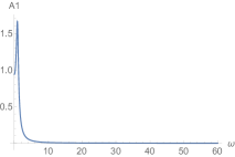
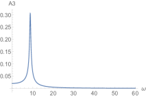
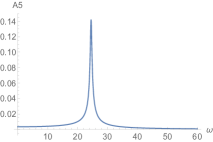
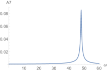
Figure 1. Plots of the functions $\omega\mapsto A_{k}(\omega)$ in (53) for $k=1,3,5,7$.

It turns out that these functions all have a steep spike close to their maximum but elsewhere they are fairly small, of several orders of magnitude less. The height of the spikes is decreasing with respect to $k$ and the maximum is moving to the right (larger $\omega$).

We are now in position to give an answer to question (a). For a given $\omega>0$, the prevailing mode $w_{k}$ is the one maximizing $A_{k}(\omega)$. For each $\omega>0$ we numerically determine which $k$ maximizes $A_{k}(\omega)$. We consider the values $P=0$ and $P=1/2$ and we obtain the results summarized in Tables 4 and 5, where $k_{p}$ is the prevailing mode so that

$$k_{p}=k_{p}(\omega)\mbox{ is such that }A_{k_{p}}(\omega)=\max_{k}A_{k}(\omega)\,.$$

$\omega\!\in$​​	​​$(0,5.39)$​​	​$(5.39,17.48)$​​	​​$(17.48,37.17)$​​	​​$(37.17,64.64)$​​	​​$(64.64,100)$​​	​​$(100,143.1)$​​	​​$(143.1,194.2)$​​	​​$(194.2,253.1)$​​
$k_{p}$	1	3	5	7	9	11	13	15

Table 4. Prevailing mode $k_{p}$ in terms of the frequency $\omega$ (for $P=0$).

$\omega\!\in$​​	​​$(0,5.2)$​​	​$(5.2,17.26)$​​	​​$(17.26,36.92)$​​	​​$(36.92,64.4)$​​	​​$(64.4,99.7)$​​	​​$(99.7,142.9)$​​	​​$(142.9,193.9)$​​	​​$(193.9,252.8)$​​
$k_{p}$	1	3	5	7	9	11	13	15

Table 5. Prevailing mode $k_{p}$ in terms of the frequency $\omega$ (for $P=1/2$).

It appears evident that the prestressing constant $P$ does not influence too much the prevailing mode, only a slight shift of the intervals. In order to find the related wind velocity $W$, from Section 2 we recall that $\omega$ is proportional to $W$:

$$\omega=\frac{{\rm St}}{H}\,W\,.$$

6. Numerical results

For our numerical experiments, we first consider external forces $g=g(\xi,t)$ able to identify the “prevailing mode” (which should be longitudinal), then we investigate whether this longitudinal mode is stable with respect to the torsional modes. According to Definition 7, in order to emphasize torsional instability we need to find a particular solution of (39) having a torsional component which does not vanish at infinity. So, we select the longitudinal mode candidate to become the prevailing mode, that is, one of the ($L^{2}$-normalized) eigenfunctions in Proposition 1 $(i)$. Indeed, according to Table 1, the least 17 longitudinal eigenvalues are all of the kind $\mu_{m,1}$ ($m=1,...,17$) that are associated to this kind of eigenfunction. Let us denote by $L_{m}$ the associated ($L^{2}$-normalized) longitudinal eigenfunction:

$$L_{m}(x,y)=C_{m}\,\left[\big{[}\mu_{m,1}^{1/2}-(1-\sigma)m^{2}\big{]}\,\tfrac{\cosh\Big{(}y\sqrt{m^{2}+\mu_{m,1}^{1/2}}\Big{)}}{\cosh\Big{(}\ell\sqrt{m^{2}+\mu_{m,1}^{1/2}}\Big{)}}+\big{[}\mu_{m,1}^{1/2}+(1-\sigma)m^{2}\big{]}\,\tfrac{\cosh\Big{(}y\sqrt{m^{2}-\mu_{m,1}^{1/2}}\Big{)}}{\cosh\Big{(}\ell\sqrt{m^{2}-\mu_{m,1}^{1/2}}\Big{)}}\right]\sin(mx)\,,$$

where $C_{m}$ is a normalization constant, see (28). Then we consider the external force in the particular form

(54) $$g_{m}(\xi,t)=A\,b\,L_{m}(\xi)\operatorname{sn}(bt,k)\operatorname{dn}(bt,k)\,,\quad b=\sqrt{\mu_{m,1}+\frac{Sm^{4}A^{2}}{\delta^{2}}}\,,\quad k=\sqrt{\frac{Sm^{4}A^{2}}{2(\mu_{m,1}\delta^{2}+Sm^{4}A^{2})}}\,,$$

where $A>0$ has to be fixed while $\operatorname{sn}$ and $\operatorname{dn}$ are the Jacobi elliptic functions: the function $\operatorname{sn}(bt,k)\operatorname{dn}(bt,k)$ is a modification of the trigonometric sine which becomes particularly useful when dealing with Duffing equations, see [1]. This choice of $g_{m}$ only slightly modifies the form given in (12). Then we prove

Proposition 15.

Assume that $P=0$ and that $g(\xi,t)=g_{m}(\xi,t)$ for some integer $m$, as defined in (54). Then the function

$$U^{p}(\xi,t)=-\frac{A}{\delta}\,\operatorname{cn}(bt,k)\,L_{m}(\xi)$$

is a periodic solution of (39). Moreover, if $A>0$ is sufficiently small, then $U^{p}$ is the unique periodic solution of (39): in such case, the prevailing mode $U^{p}$ is torsionally stable.

Proof.

Take $b$ and $k$ as in (54) and let $a=-A/\delta$. From [11] we know that the function $z(t)=a\,\operatorname{cn}(bt,k)$ solves the problem

$$\ddot{z}(t)+\mu_{m,1}\,z(t)+Sm^{4}\,z(t)^{3}=0\,,\qquad z(0)=a\,,\qquad\dot{z}(0)=0\,.$$

Since $\frac{d}{dt}\operatorname{cn}(bt,k)=-b\operatorname{sn}(bt,k)\operatorname{dn}(bt,k)$, the function $z$ also solves

(55) $$\ddot{z}(t)+\delta\,\dot{z}(t)+\mu_{m,1}\,z(t)+Sm^{4}\,z(t)^{3}=\delta\,\dot{z}(t)=A\,b\,\operatorname{sn}(bt,k)\operatorname{dn}(bt,k)\,,\qquad z(0)=a\,,\qquad\dot{z}(0)=0\,.$$

Therefore, $z$ is a periodic solution of (55) and, in turn, the function $U^{p}(\xi,t)=z(t)\,L_{m}(\xi)$ is a periodic solution of (39).

Since $k^{2}<1/2$ in view of (54) and since $\operatorname{dn}(bt,k)^{2}+k^{2}\,\operatorname{sn}(bt,k)^{2}\equiv 1$, by the properties of the Jacobi functions (see [1]) we know that

$$\max_{t>0}\big{|}\operatorname{sn}(bt,k)\operatorname{dn}(bt,k)\big{|}=\sqrt{1-k^{2}}\,.$$

Hence, recalling that $L_{m}$ is $L^{2}$-normalized, we have

$$\sup_{t>0}\int_{\Omega}g_{m}(\xi,t)^{2}\,d\xi=A^{2}\,b^{2}\,\max_{t>0}\,\big{|}\operatorname{sn}(bt,k)\operatorname{dn}(bt,k)\big{|}^{2}=\frac{2\mu_{m,1}\delta^{2}+Sm^{4}A^{2}}{2\delta^{2}}\,A^{2}\,.$$

Therefore, if $A$ is sufficiently small, then the assumptions of Theorem 5 are fulfilled and the periodic solution of (39) is unique and torsionally stable.∎

From [11] we also know that the period $\tau$ of the forcing term (and of the solution) is given by the elliptic integral

(56) $$\tau=\frac{4}{b}\int_{0}^{\pi/2}\frac{d\varphi}{\sqrt{1-k^{2}\sin^{2}\varphi}}\,.$$

Note that for $0<k^{2}<1/2$ we have $\frac{\pi}{2}\approx 1.57<\int_{0}^{\pi/2}\frac{d\varphi}{\sqrt{1-k^{2}\sin^{2}\varphi}}<1.86$ so that $\tau$ has small variations.

For all our numerical experiments we take $P=0$ and we wish two emphasize two kinds of behaviors of the solution: existence of multiple periodic solutions and torsional instability.

Existence of multiple periodic solutions. We select one longitudinal eigenfunction $L_{m}$ associated to some eigenvalue $\mu_{m,1}$ (for $m=1,...,17$), see Table 1, and one torsional eigenfunction $T_{n}$ associated to some eigenvalue $\nu_{n,2}$ (for $n=1,2,3$), see again Table 1. We take the external force $g=g_{m}$ to be as in (54) and initial conditions (40) such as

(57) $$u(\xi,0)=\alpha L_{m}(\xi)+\beta T_{n}(\xi),\qquad u_{t}(\xi,0)=0\qquad\textrm{in }\Omega$$

for some $\alpha,\beta\in\mathbb{R}$. The uniqueness statement of Theorem 5 then shows that the solution $u=u(\xi,t)$ of (39) satisfying the initial conditions (57) necessarily has the form

$$u(\xi,t)=\phi(t)L_{m}(\xi)+\psi(t)T_{n}(\xi)$$

for some $C^{2}$-functions $\phi$ and $\psi$ satisfying the following nonlinear system of ODE’s:

(58) $$\left\{\begin{array}[]{l}\ddot{\phi}(t)+\delta\dot{\phi}(t)+\mu_{m,1}\phi(t)+Sm^{2}[m^{2}\phi(t)^{2}+n^{2}\psi(t)^{2}]\phi(t)=A\,b\,\operatorname{sn}(bt,k)\operatorname{dn}(bt,k)\\ \ddot{\psi}(t)+\delta\dot{\psi}(t)+\nu_{n,2}\psi(t)+Sn^{2}[m^{2}\phi(t)^{2}+n^{2}\psi(t)^{2}]\psi(t)=0\end{array}\right.$$

while the initial conditions (57) become

(59) $$\phi(0)=\alpha\,,\quad\psi(0)=\beta\,,\quad\dot{\phi}(0)=\dot{\psi}(0)=0\,.$$

We notice that if $\beta=0$ then the solution of (58)-(59) satisfies $\psi\equiv 0$, which means that there is no torsional component at all. When $A$ is small, Proposition 15 states that $U^{p}$ is the unique periodic solution of (39) and that $g_{m}$ in (54) makes (39) torsionally stable. Our strategy then consists in taking $\beta>0$ and studying the behavior of the solution of (58)-(59) when $A$ becomes large, aiming to emphasize multiplicity of periodic solutions.

If we take $\alpha=-A/\delta$ and $\beta=0$, then the solution of (58)-(59) is given by

$$\phi(t)=-\frac{A}{\delta}\,\operatorname{cn}(bt,k)\,,\qquad\psi(t)\equiv 0$$

while

(60) $$U^{p}(\xi,t)=-\frac{A}{\delta}\,\operatorname{cn}(bt,k)\,L_{m}(\xi)$$

is a periodic solution of (39), see Proposition 15. If it was the only periodic solution, then Theorem 9 would ensure that $(\phi-U^{p},\psi)(t)\to 0$ uniformly as $t\to\infty$ for any solution of (58). Hence, in order to display multiple periodic solutions of (39) it suffices to exhibit a solution of (58) that does not satisfy this condition.

In Figure 2 we display the graphs of $U^{p}$ and of the solution $(\phi,\psi)$ of (58)-(59) with

(61) $$m=2\,,\ n=1\,,\ \delta=0.58\,,\ S=279\,,\ A=0.2645\,,\ b\mbox{ as in \eqref{fpart}}\,,\ \alpha=0\,,\ \beta=0.01\,.$$

Note that the “frequency” of $\psi$ is considerably larger than the frequency of $\phi$. This is due to the fact that $\nu_{1,2}\gg\mu_{2,1}$, see Table 1.

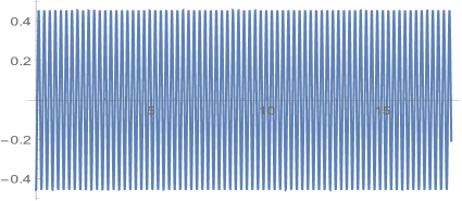
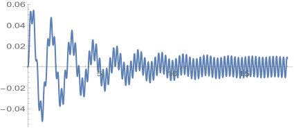
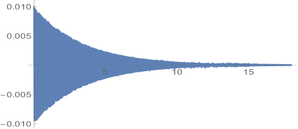
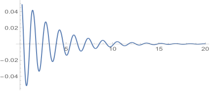
Figure 2. Plot of the functions $U^{p}$ in (60) (top left), $\phi$ (top right) and $\psi$ (bottom left) solving (58)-(59), and $t\mapsto\phi(t)-\phi(t-\tau)$ (bottom right), when (61) holds.

It appears also quite visible that $\phi-U^{p}$ does not converge uniformly to $0$, see in particular the amplitudes on the vertical axis. In the bottom right picture of Figure 2 we plot the graph of $\phi(t)-\phi(t-\tau)$, where $\tau$ is as in (56), that is, the period of the force $g_{m}$ in (54) and in (58). This plot seems to say that $\phi$ is converging to a periodic regime and this would prove that the attractor of (39) consists of at least two periodic solutions. Moreover, since $\psi\to 0$ uniformly (bottom left plot in Figure 2), this would prove that “multiplicity of periodic solutions and torsional instability are not equivalent facts”.

Finally, it is worth emphasizing that, by perturbing slightly the initial data $\alpha=-A/\delta$ and $\beta=0$ in (59), it was quite evident that the periodic solution $U^{p}$ was unstable, the $\phi$-component always behaved as in the top right picture of Figure 2 for large $t$.

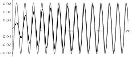
Figure 3. The functions $U^{p}$ in (60) (gray) and $\phi$ (black) solving (58)-(59) when (62) holds.

We then diminished the amplitude $A$, modified $b$ according to (54), and maintained all the other parameters as in (61); we took

(62) $$m=2\,,\ n=1\,,\ \delta=0.58\,,\ S=279\,,\ A=0.018\,,\ b\mbox{ as in \eqref{fpart}}\,,\ \alpha=0\,,\ \beta=0.01\,.$$

In Figure 3 we plot both the graphs of $U^{p}$ in (60) (gray) and $\phi$ solving (58)-(59) (black). It appears that now $\phi$ approaches very quickly $U^{p}$. This probably means that the amplitude $A$ is sufficiently small so that Theorem 9 applies and $U^{p}$ is the unique (and hence, stable) periodic solution. Note that the frequency is considerably smaller than in the plots of Figure 2.

We performed several other experiments for different couples of integers $(m,n)$, thereby changing the modes involved in the stability analysis, and we always found qualitatively similar results: two periodic solutions for large $A$ and a (probably) unique periodic solution for small $A$.

Torsional instability. We were not able to detect any torsional instability for (58), even by taking very large $A$. The reason seems to be that taking $b$ as in (54) leaves too little freedom: the frequency is directly related to the amplitude. And large frequencies are difficult to handle numerically due to large values of the derivatives of the solutions. Therefore, we considered the more standard problem

(63) $$\left\{\begin{array}[]{l}\ddot{\phi}(t)+\delta\dot{\phi}(t)+\mu_{m,1}\phi(t)+Sm^{2}[m^{2}\phi(t)^{2}+n^{2}\psi(t)^{2}]\phi(t)=A\,\sin(\omega t)\\ \ddot{\psi}(t)+\delta\dot{\psi}(t)+\nu_{n,2}\psi(t)+Sn^{2}[m^{2}\phi(t)^{2}+n^{2}\psi(t)^{2}]\psi(t)=0\end{array}\right.$$

for some mutually independent values of the amplitude $A$ and of the frequency $\omega$. In the left plot of Figure 4 we depict the graph of the $\psi$-component of the solution $(\phi,\psi)$ of (63) and (59) with the following choice of the parameters

(64) $$m=2\,,\ n=2\,,\ \delta=0.4\,,\ S=250\,,\ A=62500\,,\ \omega=275\,,\ \alpha=0\,,\ \beta=0.01\,.$$

One clearly sees that $\psi(t)\not\to 0$ as $t\to\infty$, which means torsionally instability. We performed several other experiments by considering different couples $(m,n)$ and obtained qualitatively the same graph with $\psi$ growing up in some disordered way. We plotted the graphs of $s\mapsto\psi(t)-\psi(t-2k\pi/\omega)$ (for some $k$) that also displayed a fairly disordered behavior, showing that no periodicity seems to appear. If confirmed, this would show that the $\omega$-limit set of (39) does not only contain periodic solutions for large $g$.

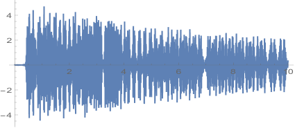
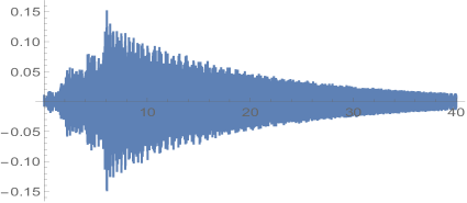
Figure 4. Left: plot of the $\psi$-component of the solution of (58)-(59) when (64) holds. Right: local torsional instability and eventual stability obtained when (65) holds.

Local torsional instability and eventual stability. The classification of Definition 7 is mathematically exhaustive since a force $g$ makes the system either torsionally stable or torsionally unstable. However, some forces making the system stable may still be dangerous from a physical (engineering) point of view and we need to focus our attention to a particular class of solutions.

Definition 16 (Local torsional instability and eventual stability).

We say a solution $u$ of (39) is locally torsionally unstable and eventually stable if

$$\lim_{t\to\infty}(\|u_{t}^{T}(t)\|_{L^{2}}+\|u^{T}(t)\|_{H^{2}_{*}})=0$$

and if one of its torsional Fourier coefficients, say $h_{n}=h_{n}(t)$, satisfies

$$\dot{h}_{n}(0)=0\,,\quad|h_{n}(t)|>10\,|h_{n}(0)|\geq 0.1\mbox{ for some }t>0\,.$$

This means that, although all the torsional components of the solution tend asymptotically to $0$, the amplitude of one torsional component has grown of at least one order of magnitude at some time $t$ compared to the initial datum which was bounded away from zero: moreover, this is not due to the initial kinetic datum $\dot{h}_{n}(0)$ since it is set to zero.

In the right picture of Figure 4 one sees an example of this situation: we depict there the graph of the $\psi$-component of the solution of (63) and (59) with the following values of the parameters

(65) $$m=4\,,\ n=2\,,\ \delta=0.12\,,\ S=258\,,\ A=6400\,,\ \omega=160.8\,,\ \alpha=0\,,\ \beta=0.01\,.$$

It appears that $\psi(t)$ grows up until about $0.15$, that is, 15 times as much as its initial value. Then it tends to vanish as $t\to\infty$.

7. Energy estimates

In this section we use the family of energies

$$E_{\alpha}(t):=\frac{1}{2}\|u_{t}(t)\|_{L^{2}}^{2}+\frac{1}{2}\|u(t)\|_{H^{2}_{*}}^{2}-\frac{P}{2}\|u_{x}(t)\|_{L^{2}}^{2}+\frac{S}{4}\|u_{x}(t)\|_{L^{2}}^{4}+\alpha\int_{\Omega}u(\xi,t)u_{t}(\xi,t)\,d\xi,$$

where $\alpha>0$, and we derive bounds for $E_{\alpha}$. The aim is to obtain bounds for the solutions of (39) from the energy bounds. Before starting, let us rigorously justify once forever the computations that follow. The regularity of weak solutions does not allow to take $v=u_{t}$ in (42). Therefore, we need to justify the differentiation of the energies $E_{\alpha}$, a computation that we use throughout the paper. In this respect, let us recall a general result, see [37, Lemma 4.1].

Lemma 17.

Let $(V,H,V^{\prime})$ be a Hilbert triple. Let $a$ be a coercive bilinear continuous form on $V$, associated with the continuous isomorphism $A$ from $V$ to $V^{\prime}$ such that $a(u,v)=\langle Au,v\rangle$ for all $u,v\in V$. If $w$ is such that

$$w\in L^{2}(0,T;V)\,,\quad w_{t}\in L^{2}(0,T;H)\,,\quad w_{tt}+Aw\in L^{2}(0,T;H)\,,$$

then, after modification on a set of measure zero, $w\in C^{0}([0,T],V)$, $w_{t}\in C^{0}([0,T],H)$ and, in the sense of distributions on $(0,T)$,

$$\langle w_{tt}+Aw,w_{t}\rangle=\frac{1}{2}\frac{d}{dt}\big{(}\|w_{t}\|_{L^{2}}^{2}+a(w,w)\big{)}\,.$$

We may now derive some energy bounds in terms of $g_{\infty}$, see (47).

Lemma 18.

Assuming that $0\leq P<\lambda_{1}$ and that $u$ is a solution of (39), we have

1. for $\delta^{2}\leq 4(\lambda_{1}-P)$,

   (66) $$E_{\delta/2}(\infty):=\limsup_{t\to\infty}E_{\delta/2}(t)\leq\frac{2\,g_{\infty}^{2}}{\delta^{2}}\,,$$

2. for $\delta^{2}\geq 4(\lambda_{1}-P)$,

   $$E_{\mu}(\infty):=\limsup_{t\to\infty}E_{\mu}(t)\leq\frac{g_{\infty}^{2}}{2(\lambda_{1}-P)}\,,$$

   where $\mu:=\frac{\delta}{2}-\frac{1}{2}\sqrt{\delta^{2}-4(\lambda_{1}-P)}$.

Proof.

Take any $\alpha\in(0,\frac{2}{3}\delta)$. From the definition of $E_{\alpha}$ and, by using Lemma 17 and (39), we infer that

$$\begin{array}[]{rl}\dot{E}_{\alpha}(t)+\alpha E_{\alpha}(t)=&\!\!\!\!\!\displaystyle\left(\frac{3\alpha}{2}-\delta\right)\|u_{t}(t)\|_{L^{2}}^{2}-\frac{\alpha}{2}\|u(t)\|_{H^{2}_{*}}^{2}+\frac{\alpha P}{2}\|u_{x}(t)\|_{L^{2}}^{2}-\frac{3S\alpha}{4}\|u_{x}(t)\|_{L^{2}}^{4}\\ &\!\!\!\!\!\displaystyle+\alpha(\alpha-\delta)\int_{\Omega}u(\xi,t)u_{t}(\xi,t)\,d\xi+\int_{\Omega}g(\xi,t)\big{(}u_{t}(\xi,t)+\alpha u(\xi,t)\big{)}\,d\xi\,.\end{array}$$

Hence, by using (17) and the Young inequality, we obtain

(69) $$\begin{array}[]{rl}\dot{E}_{\alpha}(t)+\alpha E_{\alpha}(t)\leq&\displaystyle\left(\frac{3\alpha}{2}-\delta+\gamma\right)\|u_{t}(t)\|_{L^{2}}^{2}-\frac{\alpha}{2\lambda_{1}}(\lambda_{1}-P-2\alpha\gamma)\|u(t)\|_{H^{2}_{*}}^{2}\\ &\displaystyle+\alpha(\alpha-\delta+2\gamma)\int_{\Omega}u(\xi,t)u_{t}(\xi,t)\,d\xi\,+\frac{1}{4\gamma}\|g(t)\|_{L^{2}}^{2},\end{array}$$

for every $\gamma>0$. To get a global estimate, we seek $\gamma>0$ such that

(i) $\frac{3}{2}\alpha-\delta+\gamma\leq 0$,  (ii) $\lambda_{1}-P\geq 2\alpha\gamma$,  (iii) $\alpha-\delta+2\gamma=0$.

These three conditions are satisfied if we choose

$$\begin{array}[]{lll}\displaystyle\alpha=\frac{\delta}{2}\,,&\displaystyle\gamma=\frac{\delta}{4}\,,&\mbox{if }\delta^{2}\leq 4(\lambda_{1}-P)\\ \displaystyle\alpha=\mu\,,&\displaystyle\gamma=\frac{\delta+\sqrt{\delta^{2}-4(\lambda_{1}-P)}}{4}\,,&\mbox{if }\delta^{2}\geq 4(\lambda_{1}-P)\,.\end{array}$$

Then, by using (i)-(ii)-(iii) we see that (69) entails

$$\dot{E}_{\alpha}(t)+\alpha E_{\alpha}(t)\leq\frac{1}{4\gamma}\|g(t)\|_{L^{2}}^{2},$$

and this implies, for all $t_{0}>0$, that

$$E_{\alpha}(t)\leq\,{\rm e}^{-\alpha(t-t_{0})}E_{\alpha}(t_{0})+\frac{\left(1-{\rm e}^{-\alpha(t-t_{0})}\right)}{4\alpha\gamma}\sup_{t\geq t_{0}}\|g(t)\|_{L^{2}}^{2}.$$

By letting $t\to\infty$, we deduce that

(70) $$E_{\alpha}(\infty):=\limsup_{t\to\infty}E_{\alpha}(t)\leq\frac{g_{\infty}^{2}}{4\alpha\gamma}\,.$$

The conclusions follow from (70) and the respective choices of $\alpha$ and $\gamma$ according to the size of $\delta$. ∎

Next we show that a bound on $E_{\alpha}(t)$ gives asymptotic bounds on all the norms of the solution. We start with $L^{2}$-bounds on $u$ and $u_{x}$ which are uniform in time. As it will become clear from the proofs, we can assume that $E_{\alpha}(\infty)\geq 0$.

Lemma 19 ($L^{2}$-bound on $u$).

Assume that $0\leq P<\lambda_{1}$, that $\limsup_{t\to\infty}\|g(t)\|_{L^{2}}<\infty$ and that $u$ is a solution of (39). Let $\alpha$ and $E_{\alpha}(\infty)$ be as in Lemma 18, then

(71) $$\limsup_{t\to\infty}\|u(t)\|^{2}_{L^{2}}\leq\frac{4E_{\alpha}(\infty)}{\sqrt{(\lambda_{1}-P)^{2}+4SE_{\alpha}(\infty)}+(\lambda_{1}-P)}=:\Psi\,.$$

Proof.

Let $\alpha$ be as in Lemma 18 and observe that

$$E_{\alpha}(t)=\frac{\alpha}{2}\frac{d}{dt}\|u(t)\|^{2}_{L^{2}}+\frac{1}{2}\|u_{t}(t)\|^{2}_{L^{2}}+\frac{1}{2}\|u(t)\|_{H^{2}_{*}}^{2}-\frac{P}{2}\|u_{x}(t)\|_{L^{2}}^{2}+\frac{S}{4}\|u_{x}(t)\|_{L^{2}}^{4}\,.$$

From Lemma 18 we know that there exist $C,t_{0}>0$ such that $E_{\alpha}(t)\leq C$ for all $t\geq t_{0}$. Then, setting $\Upsilon(t):=\frac{1}{2}\|u(t)\|^{2}_{L^{2}}$, the previous inequality and (17) imply that

(72) $$\alpha\dot{\Upsilon}(t)+(\lambda_{1}-P)\Upsilon(t)+S\Upsilon(t)^{2}\leq C\qquad\forall t\geq t_{0}\,.$$

Two cases may occur. If there exists $\bar{t}\geq t_{0}$ such that

(73) $$\Upsilon(\bar{t})\leq\frac{\sqrt{(\lambda_{1}-P)^{2}+4SC}-(\lambda_{1}-P)}{2S}=:\overline{\Upsilon}\,,$$

then from (72) we see that, necessarily, $\Upsilon(t)\leq\overline{\Upsilon}$ for all $t\geq\bar{t}$ since $\dot{\Upsilon}(t)<0$ whenever $\Upsilon(t)>\overline{\Upsilon}$. If there exist no $\bar{t}\geq t_{0}$ such that (73) holds, then $\dot{\Upsilon}(t)<0$ for all $t\geq t_{0}$ and $\Upsilon(t)$ has a limit at infinity, necessarily $\overline{\Upsilon}$. Therefore, in any case we have that

$$\limsup_{t\to\infty}\Upsilon(t)\leq\overline{\Upsilon}\,.$$

By applying this argument for all $t_{0}$ (so that the bound $C$ approaches $E_{\alpha}(\infty)$ when $t_{0}\to\infty$) and by recalling the definition of $\Upsilon(t)$, we obtain (71).∎

Lemma 20 ($L^{2}$-bound on $u_{x}$).

Assume that $0\leq P<\lambda_{1}$, that $\limsup_{t\to\infty}\|g(t)\|_{L^{2}}<\infty$ and that $u$ is a solution of (39). Let $\alpha$ and $E_{\alpha}(\infty)$ be as in Lemma 18 and $\Psi$ be as in (71). Then

(74) $$\limsup_{t\to\infty}\|u_{x}(t)\|_{L^{2}}^{2}\leq\frac{4E_{\alpha}(\infty)+2\alpha^{2}\Psi}{\sqrt{(\lambda_{1}-P)^{2}+2S(2E_{\alpha}(\infty)+\alpha^{2}\Psi)}+(\lambda_{1}-P)}\,.$$

Proof.

Let us rewrite $E_{\alpha}$ as

$$E_{\alpha}(t)=\frac{1}{2}\int_{\Omega}\left(\alpha u(\xi,t)+u_{t}(\xi,t)\right)^{2}d\xi-\frac{\alpha^{2}}{2}\|u(t)\|^{2}_{L^{2}}+\frac{1}{2}\|u(t)\|_{H^{2}_{*}}^{2}-\frac{P}{2}\|u_{x}(t)\|_{L^{2}}^{2}+\frac{S}{4}\|u_{x}(t)\|_{L^{2}}^{4}\,.$$

Therefore, by dropping the squared integral, we obtain

(75) $$\frac{1}{2}\|u(t)\|_{H^{2}_{*}}^{2}-\frac{P}{2}\|u_{x}(t)\|_{L^{2}}^{2}+\frac{S}{4}\|u_{x}(t)\|_{L^{2}}^{4}\leq E_{\alpha}(t)+\frac{\alpha^{2}}{2}\|u(t)\|^{2}_{L^{2}}\,.$$

Using (17) into (75), we obtain

$$\frac{S}{4}\|u_{x}(t)\|_{L^{2}}^{4}+\frac{\lambda_{1}-P}{2}\|u_{x}(t)\|_{L^{2}}^{2}\leq E_{\alpha}(t)+\frac{\alpha^{2}}{2}\|u(t)\|^{2}_{L^{2}}\,.$$

By solving this biquadratic inequality and by taking the limsup, we obtain (74). ∎

Lemma 21 ($L^{2}$-bound on $u_{t}$).

Assume that $0\leq P<\lambda_{1}$, that $\limsup_{t\to\infty}\|g(t)\|_{L^{2}}<\infty$ and that $u$ is a solution of (39). Let $\alpha$ and $E_{\alpha}(\infty)$ be as in Lemma 18 and $\Psi$ be as in (71). Then, for every $\lambda>0$,

(76) $$\limsup_{t\to\infty}\|u_{t}(t)\|_{L^{2}}^{2}\leq\frac{1+\lambda}{\lambda}\left(2E_{\alpha}(\infty)+\max_{s\in[0,\Psi]}\left(((\lambda+1)\alpha^{2}-(\lambda_{1}-P))s-\frac{S}{2}s^{2}\right)\right).$$

Proof.

The Minkowski inequality yields

$$\left(\int_{\Omega}u_{t}^{2}(\xi,t)\,d\xi\right)^{1/2}\leq\left(\int_{\Omega}\left(\alpha u(\xi,t)+u_{t}(\xi,t)\right)^{2}d\xi\right)^{1/2}+\alpha\left(\int_{\Omega}u^{2}(\xi,t)\,d\xi\right)^{1/2}\,.$$

Moreover, by using the expression of the energy and (17), we see that

$$\|u_{t}(t)\|_{L^{2}}\leq\left(2E_{\alpha}(t)-(\lambda_{1}-P-{\alpha^{2}})\|u(t)\|^{2}_{L^{2}}-\frac{S}{2}\|u(t)\|_{L^{2}}^{4}\right)^{1/2}+\alpha\|u(t)\|_{L^{2}}$$

for all $t\geq t_{0}$. Applying Young’s inequality, this yields for every $\lambda>0$

$$\|u_{t}(t)\|_{L^{2}}^{2}\leq\frac{1+\lambda}{\lambda}\left(2E_{\alpha}(t)+(\lambda\alpha^{2}-(\lambda_{1}-P-{\alpha^{2}}))\|u(t)\|^{2}_{L^{2}}-\frac{S}{2}\|u(t)\|_{L^{2}}^{4}\right).$$

∎

Lemma 22 ($H^{2}$-bound on $u$).

Assume that $0\leq P<\lambda_{1}$, that $\limsup_{t\to\infty}\|g(t)\|_{L^{2}}<\infty$ and that $u$ is a solution of (39). Let $\alpha$ and $E_{\alpha}(\infty)$ be as in Lemma 18, let $\Psi$ be as in (71). Then we have

(77) $$\limsup_{t\to\infty}\|u(t)\|_{H^{2}_{*}}^{2}\leq\frac{2\lambda_{1}}{\lambda_{1}-P}\left(E_{\alpha}(\infty)+\frac{\alpha^{2}\,\Psi}{2}\right)\,.$$

Proof.

By using (17), we see that (75) yields

$$\frac{\lambda_{1}-P}{2\lambda_{1}}\|u(t)\|_{H^{2}_{*}}^{2}\leq E_{\alpha}(t)+\frac{\alpha^{2}}{2}\|u(t)\|^{2}_{L^{2}}-\frac{S}{4}\|u(t)\|_{L^{2}}^{4}\leq E_{\alpha}(t)+\frac{\alpha^{2}}{2}\|u(t)\|^{2}_{L^{2}}$$

so that, by taking the limsup and using Lemma 19, we obtain (77).∎

We conclude this section by noticing that all the bounds obtained so far can be used for the weak solutions of the linear problem

(81) $$\left\{\begin{array}[]{rl}w_{tt}+\delta w_{t}+\Delta^{2}w+Pw_{xx}-bw=h(\xi,t)&\textrm{in }\Omega\times(0,T)\\ w=w_{xx}=0&\textrm{on }\{0,\pi\}\times[-\ell,\ell]\\ w_{yy}+\sigma w_{xx}=w_{yyy}+(2-\sigma)w_{xxy}=0&\textrm{on }[0,\pi]\times\{-\ell,\ell\},\end{array}\right.$$

obtained by taking $S=0$ in (39) and inserting the additional zero order term $bw$ (that will appear naturally while deriving the exponential decay of the solutions of the nonlinear equation). More precisely, we have

Lemma 23.

Let $h\in C^{0}(\mathbb{R}_{+},L^{2}(\Omega))$. For any weak solution $w$ of (81), we have the estimates

• ($L^{2}$ bound on $w_{t}$)

  (82) $$\limsup_{t\to\infty}\|w_{t}(t)\|_{L^{2}}^{2}\leq\frac{2}{\lambda_{1}-P-b}\limsup_{t\to\infty}\|h(t)\|_{L^{2}}^{2},$$

• ($H^{2}$ bound on $w$)

  (83) $$\limsup_{t\to\infty}\|w(t)\|_{H^{2}_{*}}^{2}\leq\frac{\lambda_{1}}{\lambda_{1}-P-b}\left(\max\Big{(}\frac{4}{\delta^{2}},\frac{1}{\lambda_{1}-P-b}\Big{)}+\frac{1}{\lambda_{1}-P-b}\right)\limsup_{t\to\infty}\|h(t)\|_{L^{2}}^{2}.\\$$

8. Proof of Theorem 5

Local and global existence of weak solution of (39)-(40) are proved in [15, Theorem 3]. Here, inspired by the work of Ball [5, Theorem 4], we prove that this solution is a strong solution in case the initial data and the forcing term are slightly more regular, that is, the second part of Theorem 5.

Proposition 24.

Let $u_{0}\in H^{4}\cap H^{2}_{*}(\Omega)$, $v_{0}\in H^{2}_{*}(\Omega)$, $T>0$ and $g\in C^{1}([0,T],L^{2}(\Omega))$. Then the unique weak solution $u$ of (39)-(40) satisfies

$$u\in C([0,T],H^{4}\cap H^{2}_{*}(\Omega))\cap C^{1}([0,T],H^{2}_{*}(\Omega))\cap C^{2}([0,T],L^{2}(\Omega)).$$

Proof.

We label the eigenfunctions $w_{j}$ of (15) with a unique index $j$ and, for all integer $k\geq 1$, we set $E_{k}=\textrm{span}(w_{1},\dots,w_{k})$ and we consider the orthogonal projection $Q_{k}:H^{2}_{*}(\Omega)\to E_{k}$. We set up the weak formulation restricted to test functions $v\in E_{k}$, namely we seek $u_{k}\in C^{2}([0,T],E_{k})$ that satisfies

(86) $$\left\{\begin{array}[]{r}((u_{k})_{tt},v)_{L^{2}}+\delta((u_{k})_{t},v)_{L^{2}}+({u_{k},v})_{H^{2}_{*}}+[-P+S\int_{\Omega}(u_{k})_{x}^{2}]({(u_{k})_{x},v_{x}})_{L^{2}}=({g,v})_{L^{2}}\\ u_{k}(0)=Q_{k}u_{0},\quad(u_{k})_{t}(0)=Q_{k}v_{0}\end{array}\right.$$

for all $v\in E_{k}$ and all $t>0$. The coordinates of $u_{k}$ in the basis $(w_{i})$, given by $u^{k}_{i}=(u_{k},w_{i})_{L^{2}}$, are time-dependent functions and from (86) we see that they solve the following systems of ODE’s, for $i=1,\ldots,k$:

(89) $$\left\{\begin{array}[]{r}(u^{k}_{i})_{tt}(t)+\delta(u^{k}_{i})_{t}(t)+\lambda_{i}u^{k}_{i}(t)+m_{i}^{2}\left[-P+S\sum_{j=1}^{k}m_{j}^{2}u^{k}_{j}(t)^{2}\right]u^{k}_{i}(t)=({g(t),w_{i}})_{L^{2}}\,,\\ u^{k}_{i}(0)=(u_{0},w_{i})_{L^{2}},\quad(u^{k}_{i})_{t}(0)=(v_{0},w_{i})_{L^{2}}\,.\end{array}\right.$$

Since the nonlinearity is analytic, from the classical theory of ODEs, we know that (89) has a unique solution for each $i=1,\ldots,k$ and that it can be extended to all $[0,T]$. Therefore (86) has a unique solution $u_{k}\in C^{2}([0,T],E_{k})$, given by

(90) $$u_{k}(\xi,t)=\sum_{i=0}^{k}u^{k}_{i}(t)w_{i}(\xi)\,.$$

Since $v_{0}\in H^{2}_{*}(\Omega)$, and from the ODE in (86) we obtain that

(91) $$\|(u_{k})_{t}(0)\|_{H^{2}_{*}}\ \ \text{and}\ \ \|(u_{k})_{tt}(0)\|_{L^{2}}\ \ \text{are uniformly bounded}.$$

Then we differentiate (86) with respect to $t$, we take $v=(u_{k})_{tt}$ and we infer that

(92) $$\frac{1}{2}\frac{d}{dt}\left(\|(u_{k})_{tt}\|_{L^{2}}^{2}+\|(u_{k})_{t}\|_{H^{2}_{*}}^{2}\right)+\delta\|(u_{k})_{tt}\|_{L^{2}}^{2}=\left(g_{t},(u_{k})_{tt}\right)_{L^{2}}+\vspace{5pt}\\ +\left(-P(u_{k})_{xxt}+\left(S\int_{\Omega}((u_{k})_{x})^{2}\right)(u_{k})_{xxt}+2S\left((u_{k})_{x},(u_{k})_{xt}\right)_{L^{2}}(u_{k})_{xx},(u_{k})_{tt}\right)_{L^{2}}\vspace{5pt}\\ \leq\|g_{t}\|_{L^{2}}\|(u_{k})_{tt}\|_{L^{2}}+\left(P+S\|(u_{k})_{x}\|_{L^{2}}^{2}\right)\|(u_{k})_{xxt}\|_{L^{2}}\|(u_{k})_{tt}\|_{L^{2}}\vspace{5pt}\\ +2S\|(u_{k})_{x}\|_{L^{2}}\|(u_{k})_{xt}\|_{L^{2}}\|(u_{k})_{xx}\|_{L^{2}}\|(u_{k})_{tt}\|_{L^{2}}\leq\|g_{t}\|_{L^{2}}\|(u_{k})_{tt}\|_{L^{2}}+C\|(u_{k})_{t}\|_{H^{2}_{*}}\|(u_{k})_{tt}\|_{L^{2}},$$

where, for the last inequality we have used the Poincaré inequality $\|(u_{k})_{xt}\|_{L^{2}}\leq C\|(u_{k})_{t}\|_{H^{2}_{*}}$ and that $\|(u_{k})_{x}\|_{L^{2}}$ and $\|(u_{k})_{xx}\|_{L^{2}}$ are uniformly bounded with respect to $t\in[0,T]$. For the latter, it is proved in [15, p. 6318] that $u_{k}$ is uniformly bounded in $C([0,T],H^{2}_{*}(\Omega))$. Then, using Young’s inequality, we infer that

(93) $$\frac{1}{2}\frac{d}{dt}\left(\|(u_{k})_{tt}\|_{L^{2}}^{2}+\|(u_{k})_{t}\|_{H^{2}_{*}}^{2}\right)+\frac{\delta}{2}\|(u_{k})_{tt}\|_{L^{2}}^{2}\leq\frac{1}{2\delta}\|g_{t}\|_{L^{2}}^{2}+C\|(u_{k})_{t}\|_{H^{2}_{*}}\|(u_{k})_{tt}\|_{L^{2}}.$$

Hence, from (91) and Gronwall Lemma, we infer that

$$\|(u_{k})_{tt}\|_{L^{2}}^{2}\ \ \text{and}\ \ \|(u_{k})_{t}\|_{H^{2}_{*}}^{2}\ \ \text{are uniformly bounded for all $t\in[0,T]$}$$

and, by the equation

$$\Delta^{2}u_{k}=-(u_{k})_{tt}-\delta(u_{k})_{t}+[p-S\int_{\Omega}(u_{k})_{x}^{2}](u_{k})_{xx}+Q_{k}g$$

we obtain that $\Delta^{2}u_{k}$ is uniformly bounded in $L^{2}(\Omega)$ for all $t\in[0,T]$ and then that $u_{k}$ is uniformly bounded in $H^{4}(\Omega)$ for all $t\in[0,T]$. At this point we can proceed as in the proof of [15, Theorem 3], starting from p.6318, to finish the proof. ∎

9. Proof of Theorem 6

We look at the PDE as the infinite dimensional dynamical system (45) where the coefficients $g_{k}$ are defined by (43). Let

$$g^{n}(\xi,t)=\sum_{k=1}^{n}g_{k}(t)w_{k}(\xi)\,.$$

We aim first to prove the existence of a periodic solution for this finite approximation of the forcing term and therefore deal with the infinite system

(94) $$\ddot{h}_{k}(t)+\delta\dot{h}_{k}(t)+\lambda_{k}h_{k}(t)+m_{k}^{2}\left[-P+S\sum_{j=1}^{\infty}m_{j}^{2}h_{j}(t)^{2}\right]h_{k}(t)=g_{k}(t)\quad\text{ for }k=1,\ldots,n$$

(95) $$\ddot{h}_{k}(t)+\delta\dot{h}_{k}(t)+\lambda_{k}h_{k}(t)+m_{k}^{2}\left[-P+S\sum_{j=1}^{\infty}m_{j}^{2}h_{j}(t)^{2}\right]h_{k}(t)=0\quad\text{ for }k\geq n+1.$$

This is equivalent to look for a weak periodic solution $u^{n}$ of the PDE

(99) $$\left\{\begin{array}[]{rl}u_{tt}+\delta u_{t}+\Delta^{2}u+\left[P-S\int_{\Omega}u_{x}^{2}\right]u_{xx}=g^{n}(\xi,t)&\textrm{in }\Omega\times(0,\tau)\\ u=u_{xx}=0&\textrm{on }\{0,\pi\}\times[-\ell,\ell]\\ u_{yy}+\sigma u_{xx}=u_{yyy}+(2-\sigma)u_{xxy}=0&\textrm{on }[0,\pi]\times\{-\ell,\ell\}.\end{array}\right.$$

Since we are only interested in existence, we can look for a time periodic solution having all components $h_{k}$ identically zero for $k\geq n+1$ and this yields, for the $n$ first components of the solution, the finite system

(100) $$\ddot{h}_{k}(t)+\delta\dot{h}_{k}(t)+\lambda_{k}h_{k}(t)+m_{k}^{2}\left[-P+S\sum_{j=1}^{n}m_{j}^{2}h_{j}(t)^{2}\right]h_{k}(t)=g_{k}(t)\quad\text{ for }k=1,\ldots,n.$$

This means that we seek a $\tau$-periodic solution $u^{n}$ of (99) in the form

(101) $$u^{n}(\xi,t):=\sum_{k=1}^{n}h_{k}(t)w_{k}(\xi).$$

The Fourier coefficients $h_{k}$ also depend on $n$ but we voluntarily write $h_{k}$ to simplify the notations.

We introduce the spaces $C_{\tau}^{2}(\mathbb{R})$ and $C_{\tau}^{0}(\mathbb{R})$ of $C^{2}$ and $C^{0}$ $\tau$-periodic scalar functions. Then we define the linear diagonal operator $L_{n}:(C_{\tau}^{2}(\mathbb{R}))^{n}\to(C_{\tau}^{0}(\mathbb{R}))^{n}$ whose $k$-th component is given by

$$L_{n}^{k}(h_{1},\ldots,h_{n})=\ddot{h}_{k}(t)+\delta\dot{h}_{k}(t)+(\lambda_{k}-m_{k}^{2}P)h_{k}(t)\qquad(k=1,\ldots,n)$$

and the potential $G_{n}$ defined by

$$G_{n}(h_{1},\ldots,h_{n})=\frac{S}{4}\sum_{j,k=1}^{n}m_{j}^{2}m_{k}^{2}h_{j}^{2}h_{k}^{2}.$$

It is also convenient to use the boldface notation $\mathbb{s}=(s_{1},\ldots,s_{n})$ for any $n$-tuple. With these notations, (100) becomes

$$L_{n}(\mathbb{h}(t))+\nabla G_{n}(\mathbb{h}(t))=\mathbb{g}(t).$$

Since $\delta>0$, for all $\mathbb{q}\in(C_{\tau}^{0}(\mathbb{R}))^{n}$ there exists a unique $\mathbb{h}\in(C_{\tau}^{2}(\mathbb{R}))^{n}$ such that $L_{n}(\mathbb{h})=\mathbb{q}$ and $\mathbb{h}$ may be found explicitly by solving the diagonal system of linear ODEs. Thanks to the compact embedding $(C_{\tau}^{2}(\mathbb{R}))^{n}\subset(C_{\tau}^{0}(\mathbb{R}))^{n}$, the inverse $L_{n}^{-1}:(C_{\tau}^{0}(\mathbb{R}))^{n}\to(C_{\tau}^{0}(\mathbb{R}))^{n}$ is a compact operator. Consider the nonlinear map $\Gamma_{n}:(C_{\tau}^{0}(\mathbb{R}))^{n}\times[0,1]\to(C_{\tau}^{0}(\mathbb{R}))^{n}$ defined by

$$\Gamma_{n}(\mathbb{h},\nu)=L_{n}^{-1}\left(\mathbb{g}-\nu\nabla G_{n}(\mathbb{h})\right)\qquad\forall(\mathbb{h},\nu)\in(C_{\tau}^{0}(\mathbb{R}))^{n}\times[0,1]\,.$$

The map $\Gamma_{n}$ is also compact and, moreover, it satisfies the following property: there exists $H_{n}>0$ (independent of $\nu$) such that if $\mathbb{h}\in(C_{\tau}^{0}(\mathbb{R}))^{n}$ solves the equation $\mathbb{h}=\Gamma_{n}(\mathbb{h},\nu)$, then

(102) $$\|\mathbb{h}\|_{(C_{\tau}^{0}(\mathbb{R}))^{n}}\leq H_{n}.$$

Indeed, by Lemma 18, any periodic solution $u$ of

(103) $$u_{tt}+\delta u_{t}+\Delta^{2}u+\left[P-\nu S\int_{\Omega}u_{x}^{2}\right]u_{xx}=g^{n}(\xi,t)\ \textrm{ in }\Omega\times(0,\tau)$$

satisfies energy bounds that do not depend on $\nu$, namely

$\diamondsuit$ for $\delta^{2}\leq 4(\lambda_{1}-P)$

$$\max_{t\in[0,\tau]}E_{\delta/2}(t)\leq\frac{2}{\delta^{2}}\max_{t\in[0,\tau]}\|g^{n}(t)\|_{L^{2}}^{2}\leq\frac{2}{\delta^{2}}\max_{t\in[0,\tau]}\|g(t)\|_{L^{2}}^{2}\,,$$

$\diamondsuit$ for $\delta^{2}\geq 4(\lambda_{1}-P)$,

$$\max_{t\in[0,\tau]}E_{\mu}(t)\leq\frac{1}{2(\lambda_{1}-P)}\max_{t\in[0,\tau]}\|g(t)\|_{L^{2}}^{2}\,,\qquad\mbox{where }\mu=\frac{\delta}{2}-\frac{1}{2}\sqrt{\delta^{2}-4(\lambda_{1}-P)}.$$

These energy bounds give $H^{2}_{*}(\Omega)$-bounds on $u$ and $L^{2}$-bound on $u_{t}$ as shown by Lemmas 21 and 22 (we use here the periodicity of $g$ and $u$). Back to the finite dimensional Hamiltonian system (100), this yields the desired $(C_{\tau}^{0}(\mathbb{R}))^{n}$-bound in (102). Hence, since the equation $\mathbb{h}=\Gamma_{n}(\mathbb{h},0)$ admits a unique solution, the Leray-Schauder principle ensures the existence of a solution $\mathbb{h}\in(C_{\tau}^{0}(\mathbb{R}))^{n}$ of $\mathbb{h}=\Gamma_{n}(\mathbb{h},1)$. This proves the existence of a $\tau$-periodic solution of the finite system (100) and, equivalently, of the PDE (99). Let us denote this solution by $u^{n}$, see (101).

To complete the proof of Theorem 6, we now show that the sequence $(u^{n})_{n}$ converges to a periodic solution $u$ of (39). Since the energy bounds on $u^{n}$ are independent of $n$, the $H^{2}_{*}$-bounds on $u^{n}$ and the $L^{2}$-bounds on $u^{n}_{t}$ are also independent of $n$. The equation in weak form

(104) $$\langle u^{n}_{tt},v\rangle+\delta(u^{n}_{t},v)_{L^{2}}+(u^{n},v)_{H^{2}_{*}}+\big{[}S\|u^{n}_{x}\|_{L^{2}}^{2}-P\big{]}(u^{n}_{x},v_{x})_{L^{2}}=(g^{n},v)_{L^{2}}\,,$$

for all $t\in[0,\tau]$ and all $v\in H^{2}_{*}(\Omega)$, then yields a $(H^{2}_{*})^{\prime}$ bound on $u^{n}_{tt}$. Up to a subsequence, we can therefore pass to the limit in the weak formulation of (99):

$$\begin{array}[]{l}u^{n}\to u\mbox{ weakly* in }L^{\infty}([0,\tau],H^{2}_{*}(\Omega)),\\ u^{n}_{t}\to u_{t}\mbox{ weakly* in }L^{\infty}([0,\tau],L^{2}(\Omega)),\\ u^{n}_{tt}\to u_{tt}\mbox{ weakly* in }L^{\infty}([0,\tau],(H^{2}_{*}(\Omega))^{\prime}).\end{array}$$

Hence, there exists a $\tau$-periodic solution $u$ of equation (5), satisfied in the sense of $L^{\infty}([0,\tau],(H^{2}_{*}(\Omega))^{\prime})$. To conclude, observe that the continuity properties of $u$ follow from Lemma 17 and therefore $u$ is also a weak solution in the sense of Definition 4.

10. Proof of Theorem 9

The proof of Theorem 9 is based on the following statement.

Lemma 25.

Assume (47). There exists $g_{0}=g_{0}(\delta,S,P,\lambda_{1})>0$ such that if

(105) $$g_{\infty}=\limsup_{t\to\infty}\|g(t)\|_{L^{2}}<g_{0},$$

then there exists $\eta>0$ such that

$$\lim_{t\to\infty}{\rm e}^{\eta t}\left(\|u_{t}(t)-v_{t}(t)\|_{L^{2}}+\|u(t)-v(t)\|_{H^{2}_{*}}\right)=0$$

for any two solutions $u$ and $v$ of (39).

Proof.

Let $\eta>0$, to be fixed later. If $u$ and $v$ are two solutions of (39), then $w=(u-v){\rm e}^{\eta t}$ is such that

$$\langle w_{tt},\varphi\rangle+(\delta-2\eta)(w_{t},\varphi)_{L^{2}}+(w,\varphi)_{H^{2}_{*}}-P(w_{x},\varphi_{x})_{L^{2}}-\eta(\delta-\eta)(w,\varphi)_{L^{2}}=(h(\xi,t){\rm e}^{\eta t},\varphi)_{L^{2}}$$

for all $t\in[0,T]$ and all $\varphi\in H^{2}_{*}(\Omega)$, where

$$h(\xi,t)=S\left(u_{xx}(\xi,t)\int_{\Omega}u_{x}^{2}(\xi,t)d\xi-v_{xx}(\xi,t)\int_{\Omega}v_{x}^{2}(\xi,t)d\xi\right).$$

To get estimates on $w$, we estimate first the $L^{2}$ norm of $h(\xi,t){\rm e}^{\eta t}$. We write

$$h(\xi,t){\rm e}^{\eta t}=S\left(u_{xx}(\xi,t){\rm e}^{\eta t}\int_{\Omega}(u_{x}^{2}-v_{x}^{2})(\xi,t)d\xi+w_{xx}(\xi,t)\int_{\Omega}v_{x}^{2}(\xi,t)d\xi\right).$$

Therefore, we have

$$\|h(t){\rm e}^{\eta t}\|_{L^{2}}\leq S\big{(}\|u_{xx}(t)\|_{L^{2}}\|w_{x}(t)\|_{L^{2}}\|u_{x}(t)+v_{x}(t)\|_{L^{2}}+\|w_{xx}(t)\|_{L^{2}}\|v_{x}(t)\|_{L^{2}}\big{)}$$

so that, by combining (17) with Lemmas 20 and 22, we deduce that there exists $K_{g}>0$ such that

(106) $$\limsup_{t\to\infty}\|h(t){\rm e}^{\eta t}\|_{L^{2}}^{2}\leq K_{g}\|w(t)\|_{H^{2}_{*}}^{2}$$

and, for a family of varying $g\in C^{0}(\mathbb{R}_{+},L^{2}(\Omega))$,

(107) $$K_{g}\to 0\qquad\mbox{if}\qquad g_{\infty}\to 0.$$

Taking into account the $H^{2}$-estimate (83) for the linear equation (81), we get

$$\limsup_{t\to\infty}\|w(t)\|_{H^{2}_{*}}^{2} \leq \frac{\lambda_{1}}{\lambda_{1}-P-\eta}\left(\max\Big{(}\frac{4}{\delta^{2}},\frac{1}{\lambda_{1}-P-\eta}\Big{)}+\frac{1}{\lambda_{1}-P-\eta}\right)\limsup_{t\to\infty}\|h(t){\rm e}^{\eta t}\|_{L^{2}}^{2}$$

by (106) $$\leq \frac{\lambda_{1}\,K_{g}}{\lambda_{1}-P-\eta}\left(\max\Big{(}\frac{4}{\delta^{2}},\frac{1}{\lambda_{1}-P-\eta}\Big{)}+\frac{1}{\lambda_{1}-P-\eta}\right)\limsup_{t\to\infty}\|w(t)\|_{H^{2}_{*}}^{2}.$$

Therefore we infer that there exists $\eta>0$ such that

(108) $$\lim_{t\to\infty}\|w(t)\|_{H^{2}_{*}}=0$$

as soon as

$$\frac{\lambda_{1}\,K_{g}}{\lambda_{1}-P-\eta}\left(\max\Big{(}\frac{4}{\delta^{2}},\frac{1}{\lambda_{1}-P-\eta}\Big{)}+\frac{1}{\lambda_{1}-P-\eta}\right)<1.$$

In view of (107) this happens provided that (105) holds for a sufficiently small $g_{0}=g_{0}(\delta,S,P,\lambda_{1})>0$. Hence, if (105) is fulfilled, then (108) holds and from (106) we deduce that also

$$\limsup_{t\to\infty}\|h(t){\rm e}^{\eta t}\|_{L^{2}}=0\,.$$

Therefore, the estimate (82) for the linear equation (81) gives

$$\limsup_{t\to\infty}\|w_{t}(t)\|_{L^{2}}=0$$

as well. Since $w_{t}=\left(\eta(u-v)+(u_{t}-v_{t})\right){\rm e}^{\eta t}$ and $\|{\rm e}^{\eta t}(u-v)\|_{L^{2}}\to 0$ by (108), the proof is complete.∎

Back to the proof of Theorem 9, assume first that $g$ is $\tau$-periodic for some $\tau>0$. Then Theorem 5 gives the existence of a $\tau$-periodic solution $U^{p}$. If $V$ is another periodic solution (of any period!), then from Lemma 25 we know that

$$\lim_{t\to\infty}{\rm e}^{\eta t}\left(\|U^{p}_{t}(t)-V_{t}(t)\|_{L^{2}}+\|U^{p}(t)-V(t)\|_{H^{2}_{*}}\right)=0$$

so that the period of $V$ is also $\tau$ and $V=U^{p}$. This proves uniqueness of the periodic solution.

Finally, assume that $g$ is even with respect to $y$. Let $U$ be a solution of (39)-(40) with initial data being purely longitudinal, that is, $U(\xi,0),U_{t}(\xi,0)\in H^{2}_{\mathcal{E}}(\Omega)$, see (32). Writing $U$ in the form (44), with its Fourier components satisfying (45), we see that the torsional Fourier components $h^{n}$ of $U$ satisfy

$$\ddot{h}^{n}(t)+\delta\dot{h}^{n}(t)+\nu h^{n}(t)+m^{2}\left[-P+S\sum_{j=1}^{\infty}m_{j}^{2}h_{j}(t)^{2}\right]h^{n}(t)=0\,,\qquad\dot{h}^{n}(0)=h^{n}(0)=0$$

since $g$ is even with respect to $y$ and its torsional Fourier components are zero. Therefore, $h^{n}(t)\equiv 0$ for all torsional Fourier coefficient $h^{n}$ and $U$ is purely longitudinal:

(109) $$U(t)=U^{L}(t)\,,\qquad U^{T}(t)\equiv 0.$$

Take now any solution $V$ of (39): then, by Lemma 25, we have

$$0 = \lim_{t\to\infty}\left(\|U_{t}(t)-V_{t}(t)\|_{L^{2}}^{2}+\|U(t)-V(t)\|_{H^{2}_{*}}^{2}\right)$$

by (109) $$= \lim_{t\to\infty}\left(\|U_{t}^{L}(t)-V_{t}(t)\|_{L^{2}}^{2}+\|U^{L}(t)-V(t)\|_{H^{2}_{*}}^{2}\right)$$

by orthogonality (32) $$= \lim_{t\to\infty}\left(\|U_{t}^{L}(t)-V_{t}^{L}(t)\|_{L^{2}}^{2}+\|V_{t}^{T}(t)\|_{L^{2}}^{2}+\|U^{L}(t)-V^{L}(t)\|_{H^{2}_{*}}^{2}+\|V^{T}(t)\|_{H^{2}_{*}}^{2}\right)$$

$$\geq \lim_{t\to\infty}\left(\|V_{t}^{T}(t)\|_{L^{2}}^{2}+\|V^{T}(t)\|_{H^{2}_{*}}^{2}\right)\,.$$

According to Definition 7 this implies that $g$ makes the system (39) torsionally stable.

11. Proof of Theorem 10

To prove Theorem 10 we follow very closely the arguments in [34, Section 2], the main difference being the presence of $b\neq 0$ in the below equation (110).

The proof of Theorem 10 is a straightforward consequence of the following statement.

Proposition 26.

There exist $T>0$ and a $T$-antiperiodic function $f\in C^{\infty}(\mathbb{R})$ such that the equation

(110) $$\ddot{v}+\dot{v}+bv+v^{3}=f(t)$$

admits at least two distinct $T$-antiperiodic solutions of class $C^{\infty}(\mathbb{R})$.

Indeed, taking Proposition 26 for granted, let $v^{1}$ and $v^{2}$ be two distinct $T-$antiperiodic solutions of (110) and set

$$u^{i}(\xi,t)=v^{i}(t)\phi(\xi)\qquad(i=1,2)$$

where $\phi\in C^{\infty}(\overline{\Omega})$ is an $L^{2}$-normalized eigenfunction of (15), associated to some eigenvalue $\lambda$. Then it is straightforward that $u^{i}$ satisfies

$$u^{i}_{tt}+\delta u^{i}_{t}+\Delta^{2}u^{i}+\left[P-S\int_{\Omega}(u^{i}_{x})^{2}\right]u^{i}_{xx}$$

$$=\phi(\xi)\big{[}\ddot{v}^{i}+\delta\dot{v}^{i}+(\lambda-Pm^{2})v^{i}+Sm^{4}(v^{i})^{3}\big{]}=\phi(\xi)f(t)\quad\textrm{in }\Omega\times(0,T)\qquad(i=1,2)\,.$$

Therefore, we have two periodic solutions of (39) for $\delta=1$, $\lambda-Pm^{2}=b$, $S=m^{-4}$, $g(\xi,t)=\phi(\xi)f(t)$. This completes the proof of Theorem 10, provided that Proposition 26 holds.

So, let us now prove Proposition 26. We suppose that $u$ and $v$ are two solutions of (110) and we set $w=v-u$. Then

$$\ddot{w}+\dot{w}+bw+w^{3}=\ddot{v}+\dot{v}+bv+v^{3}-(\ddot{u}+\dot{u}+bu+u^{3})-3v^{2}u+3vu^{2}=-3v^{2}u+3vu^{2}$$

and from the identity $3uw^{2}+3u^{2}w=3uv^{2}-3u^{2}v$ we infer that

(111) $$\ddot{w}+\dot{w}+bw+3uw^{2}+3u^{2}w+w^{3}=0.$$

So, at every point where $w\neq 0$, $u$ is a root of a second order polynomial, namely

(112) $$3u^{2}+3wu+\left(w^{2}+\frac{\ddot{w}+\dot{w}}{w}+b\right)=0,$$

whose discriminant reads

(113) $$9w^{2}-12\left(w^{2}+\frac{\ddot{w}+\dot{w}}{w}+b\right)=-12\left(\frac{w^{2}}{4}+\frac{\ddot{w}+\dot{w}}{w}+b\right).$$

To construct the appropriate source term $f(t)$, inspired by the expression (113), we start with the following local result.

Lemma 27.

There exist a real polinomial $P$ of degree $5$ and a neighborhood $V$ of $0$ such that

$$\begin{array}[]{l}P(t)t>0\ \ \text{on}\ \ V\backslash\{0\}\ \ \text{and}\ \ \dot{P}(t)>0\ \ \text{on}\ \ V,\vspace{5pt}\\ \phi_{P}(t):=\left\{\begin{array}[]{cl}-\left(\frac{P^{2}(t)}{4}+\frac{\ddot{P}(t)+\dot{P}(t)}{P(t)}+b\right)&\text{if}\ \ t\in V\backslash\{0\},\vspace{5pt}\\ 0&\text{if}\ \ t=0\end{array}\right.\qquad\text{is of class $C^{\infty}(V)$},\vspace{5pt}\\ \phi_{P}>0\ \ \text{on}\ \ V\backslash\{0\},\ \ \dot{\phi}_{P}(0)=0\ \ \text{and}\ \ \ddot{\phi}_{P}(0)>0\,.\end{array}$$

Proof.

We search for a polynomial of the form

(114) $$P(t)=t+\frac{A}{2}t^{2}+\frac{B}{6}t^{3}+\frac{C}{24}t^{4}+\frac{D}{120}t^{5},$$

where $A,B,C$ and $D$ will be suitably chosen. Observing that

$$\dot{P}(t)=1+At+\frac{B}{2}t^{2}+\frac{C}{6}t^{3}+\frac{D}{24}t^{4}\ \ \text{and}\ \ \ddot{P}(t)=A+Bt+\frac{C}{2}t^{2}+\frac{D}{6}t^{3}\,,$$

and choosing $A=-1$, we infer that

$$\begin{array}[]{rcl}\displaystyle{\frac{\ddot{P}(t)+\dot{P}(t)}{P(t)}}+b&=&\displaystyle{\frac{1+A+(A+B)t+\frac{B+C}{2}t^{2}+\frac{C+D}{6}t^{3}+\frac{D}{24}t^{4}}{t+\frac{A}{2}t^{2}+\frac{B}{6}t^{3}+\frac{C}{24}t^{4}+\frac{D}{120}t^{5}}}+b\vspace{10pt}\\ &=&\displaystyle{\frac{-1+B+b+\frac{B+C-b}{2}t+\frac{C+D+bB}{6}t^{2}+\frac{D+bC}{24}t^{3}+\frac{bD}{120}t^{4}}{1-\frac{1}{2}t+\frac{B}{6}t^{2}+\frac{C}{24}t^{3}+\frac{D}{120}t^{4}}}.\end{array}$$

So we choose $B$ and $C$ such that

$$-1+B+b=0\ \ \text{and}\ \ B+C-b=0.$$

Hence, choosing $A=-1$, $B=1-b$ and $C=2b-1$, we may write

$$\begin{array}[]{rcl}\displaystyle{\frac{P^{2}(t)}{4}+\frac{\ddot{P}(t)+\dot{P}(t)}{P(t)}+b}&=&\displaystyle{\frac{\frac{C+D+bB}{6}t^{2}+\frac{D+bC}{24}t^{3}+\frac{bD}{120}t^{4}}{1-\frac{1}{2}t+\frac{B}{6}t^{2}+\frac{C}{24}t^{3}+\frac{D}{120}t^{4}}}+\displaystyle{\frac{t^{2}}{4}\left(1-\frac{1}{2}t+\frac{B}{6}t^{2}+\frac{C}{24}t^{3}+\frac{D}{120}t^{3}\right)^{2}\vspace{10pt}}\\ &=&\displaystyle{\left(\frac{C+D+bB}{6}+\frac{1}{4}\right)t^{2}+\left(\frac{N(t)}{1-\frac{1}{2}t+\frac{B}{6}t^{2}+\frac{C}{24}t^{3}+\frac{D}{120}t^{4}}+Q(t)\right)t^{3}}\end{array}$$

where $N(t)$ and $Q(t)$ are polynomials. So, we must choose $D$ such that

$$\frac{C+D+bB}{6}+\frac{1}{4}=\frac{2C+2D+2bB+3}{12}<0.$$

With the choice $B=1-b$ and $C=2b-1$, the last inequality is equivalent to ask $D<b^{2}-3b-\frac{1}{2}$ and we may take $D=b^{2}-3b-1$. Therefore, with

$$A=-1,\ \ B=1-b,\ \ C=2b-1,\ \ D=b^{2}-3b-1$$

the polynomial $P(t)$ given by (114) satisfies all of the conditions of this lemma on a suitably small neighborhood $V$ of $0$. ∎

Proposition 28.

There exist $T>0$ and $w\in C^{\infty}(\mathbb{R})$, $T$-antiperiodic, with

1. $w>0$ on $(0,T)$,

2. $\phi(t):=\left\{\begin{array}[]{cl}-\left(\frac{w^{2}(t)}{4}+\frac{\ddot{w}(t)+\dot{w}(t)}{w(t)}+b\right)&\text{if}\ \ t\notin T\mathbb{Z},\vspace{5pt}\\ 0&\text{if}\ \ t\in T\mathbb{Z}\end{array}\right.$

   $\phi>0$ on $(0,T)$, $\phi(0)=\dot{\phi}(0)=0$, $\ddot{\phi}(0)>0$ and $\phi\in C^{\infty}(\mathbb{R})$.

Proof.

The proof is very similar to the proof of [34, Proposition 2.3] and, for the sake of completeness, we just stress the difference caused by the extra term $b$. Following the proof of [34, Proposition 2.3], everything remains unchanged except that:

1. At [34, p.1522], the definitions of $\psi$ and $\psi_{n}$ now read

   $$\psi=-\left(\frac{h^{3}}{4}+\ddot{h}+\dot{h}+bh\right)\ \ \text{and}\ \ \psi_{n}=-\left(\frac{w_{n}^{3}}{4}+\ddot{w_{n}}+\dot{w_{n}}+bw_{n}\right).$$

2. At [34, p.1523, lines 8-10], the estimate $\ddot{h}_{n}+\dot{h}_{n}\leq(\widetilde{\ddot{h}}+\widetilde{\dot{h}})\ast\rho_{n}$ now reads $\ddot{h}_{n}+\dot{h}_{n}+bh_{n}\leq(\widetilde{\ddot{h}}+\widetilde{\dot{h}}+bh)\ast\rho_{n}$.

3. At [34, p.1523, lines 13-14], the estimate $\displaystyle{(\ddot{h}_{n}+\dot{h}_{n})(t)\leq\int_{-1/n}^{+1/n}-\left[\frac{1}{4}h^{3}(t-s)+\gamma\right]\rho_{n}(s)ds}$ now reads $\displaystyle{(\ddot{h}_{n}+\dot{h}_{n}+bh_{n})(t)\leq\int_{-1/n}^{+1/n}-\left[\frac{1}{4}h^{3}(t-s)+\gamma\right]\rho_{n}(s)ds}$.

4. And finally, at [34, p.1523, eq. (2.21)], the inequality

   $${(h_{n}^{3}/4+\ddot{h}_{n}+\dot{h}_{n})(t)\leq-\gamma+\frac{1}{4}|h_{n}^{3}(t)-h^{3}(t)|+\frac{1}{4}\int_{-1/n}^{+1/n}|h^{3}(t-s)-h^{3}(t)|\rho_{n}(s)ds}$$

   now becomes

   $${(h_{n}^{3}/4+\ddot{h}_{n}+\dot{h}_{n}+bh_{n})(t)\leq-\gamma+\frac{1}{4}|h_{n}^{3}(t)-h^{3}(t)|+\frac{1}{4}\int_{-1/n}^{+1/n}|h^{3}(t-s)-h^{3}(t)|\rho_{n}(s)ds}.$$

This completes the proof.∎

We are now ready to conclude the proof of Proposition 26.

Proof of Proposition 26 completed.

Let $w$ and $\phi(t)$ be as in Proposition 28 and $\theta(t)$ be the (discontinuous) $T$-antiperiodic function such that $\theta(t)=1$ on $[0,T)$. Taking into account equations (112) and (113), we set

(115) $${u(t)=\frac{-3w(t)+\sqrt{12}\sqrt{\phi(t)}\,\theta(t)}{6}=-\frac{1}{2}w(t)+\frac{1}{\sqrt{3}}\theta(t)\sqrt{\phi(t)}}\ \ \text{and}\ \ v(t)=u(t)+w(t).$$

Observe that $\theta(t)\sqrt{\phi(t)}$ is $T$-antiperiodic and [34, Lemma 2.5] guarantees that $\theta(t)\sqrt{\phi(t)}$ is of class $C^{\infty}$. As a consequence, $u$ and $v$ are of class $C^{\infty}$ and $T$-antiperiodic. Moreover,

(116) $$\ddot{v}+\dot{v}+bv+v^{3}-(\ddot{u}+\dot{u}+bu+u^{3})=\ddot{w}+\dot{w}+bw+w^{3}+3v^{2}u-3vu^{2}=\ddot{w}+\dot{w}+bw+w^{3}+3uw^{2}+3u^{2}w.$$

Also observe that, by the definition of $u$,

$$\left(u+\frac{w}{2}\right)^{2}=u^{2}+uw+\frac{w^{2}}{4}=-\frac{1}{3}\left(\frac{w^{2}}{4}+\frac{\ddot{w}+\dot{w}}{w}+b\right)$$

and we infer from the last identity that

$$\ddot{w}+\dot{w}+bw+w^{3}+3uw^{2}+3u^{2}w=0,$$

which, combined with (116), implies that

$$\ddot{v}+\dot{v}+bv+v^{3}=\ddot{u}+\dot{u}+bu+u^{3}.$$

Then we choose $f=\ddot{u}+\dot{u}+bu+u^{3}$ and we obtain two periodic solutions. ∎

12. Proof of Theorem 11

We start this proof with a technical result.

Lemma 29.

Let $u\in C^{0}(\mathbb{R}_{+};H^{2}_{*}(\Omega))\cap C^{1}(\mathbb{R}_{+};L^{2}(\Omega))\cap C^{2}(\mathbb{R}_{+};(H^{2}_{*}(\Omega))^{\prime})$ be a weak solution of (39) as in Definition 4. Then, for all $0<t<s$, we have

$$\int_{t}^{s}\langle u^{T}_{tt}(\tau),u^{T}(\tau)\rangle d\tau=-\int_{t}^{s}\|u^{T}_{t}(\tau)\|_{L^{2}}^{2}\,d\tau+\int_{\Omega}\Big{[}u^{T}_{t}(s)u^{T}(s)-u^{T}_{t}(t)u^{T}(t)\Big{]}\,.$$

Proof.

Let $u_{k}\in C^{2}([0,T],E_{k})$ be the Galerkin sequence defined in the proof of Proposition 24. From Step 3 in the proof of [15, Theorem 3] we know that $u_{k}\to u$ in $C^{0}([0,T],H^{2}_{*}(\Omega))$ for all $T>0$. Moreover, given $T>0$, from [15, Eq. (21) and Step 3] we infer that the sequence $((u_{k})_{tt})$ is bounded in $C^{0}([0,T],(H^{2}_{*}(\Omega))^{\prime})$. Hence, up to a subsequence, $(u_{k})_{tt}(t)\rightharpoonup u_{tt}(t)$ in $(H^{2}_{*}(\Omega))^{\prime}$ for each $t$ and such convergence, as from Step 4 in the proof of [15, Theorem 3], reads

$$\langle u_{tt}(\tau),v\rangle=\lim_{k\to\infty}\int_{\Omega}(u_{k})_{tt}(\tau)v\,d\xi\ \ \text{for all}\ \ v\in H^{2}_{*}(\Omega).$$

Using the orthogonal decomposition (33) we infer that

$$\langle u^{T}_{tt}(\tau),u^{T}(\tau)\rangle=\lim_{k\to\infty}\int_{\Omega}(u_{k})^{T}_{tt}(\tau)(u_{k})^{T}(\tau)d\xi\ \ \text{for all $\tau\in[t,s]$}.$$

Whence, by the Lebesgue Dominated Convergence Theorem, the Fubini Theorem and an integration by parts, we obtain

$$\int_{t}^{s}\langle u^{T}_{tt}(\tau),u^{T}(\tau)\rangle d\tau = \int_{t}^{s}\lim_{k\to\infty}\int_{\Omega}(u_{k})^{T}_{tt}(\tau)(u_{k})^{T}(\tau)d\xi\,d\tau=\lim_{k\to\infty}\int_{t}^{s}\int_{\Omega}(u_{k})^{T}_{tt}(\tau)(u_{k})^{T}(\tau)d\xi\,d\tau$$

$$= \lim_{k\to\infty}\int_{\Omega}\int_{t}^{s}(u_{k})^{T}_{tt}(\tau)(u_{k})^{T}(\tau)d\tau\,d\xi$$

$$= \lim_{k\to\infty}\bigg{(}-\int_{t}^{s}\|(u_{k})^{T}_{t}(\tau)\|_{L^{2}}^{2}\,d\tau+\int_{\Omega}\Big{[}(u_{k})^{T}_{t}(s)(u_{k})^{T}(s)-(u_{k})^{T}_{t}(t)(u_{k})^{T}(t)\Big{]}\bigg{)}$$

$$= -\int_{t}^{s}\|u^{T}_{t}(\tau)\|_{L^{2}}^{2}\,d\tau+\int_{\Omega}\Big{[}u^{T}_{t}(s)u^{T}(s)-u^{T}_{t}(t)u^{T}(t)\Big{]}$$

and the result follows.∎

Then we establish an exponentially fast convergence result for a related linear problem. The exponential decay is obtained in three steps: first we prove that the liminf of the norms of the solution tends to 0, then we prove that the limit of the norms tends to 0 which, finally, allows us to argue as in [17] to infer the exponential decay. We point out that we deal with a PDE and not with an ODE as in [17, Lemma 3.7].

Lemma 30.

Assume that the continuous function $a=a(t)$ satisfies $a\geq 0$ and $a_{\infty}:=\limsup_{t\to\infty}a(t)<\infty$. Assume that

$$\delta>\max\left\{2,\frac{\nu_{1,2}\,a_{\infty}^{2}}{\gamma(2\nu_{1,2}-P)}\right\},$$

where $\gamma$ is the optimal constant for inequality (20), and let

$$u\in C^{0}(\mathbb{R}_{+};H^{2}_{*}(\Omega))\cap C^{1}(\mathbb{R}_{+};L^{2}(\Omega))\cap C^{2}(\mathbb{R}_{+};(H^{2}_{*}(\Omega))^{\prime})$$

be a weak solution of (39) (see Definition 4) such that

(117) $$\langle u^{T}_{tt},v\rangle+\delta(u^{T}_{t},v)_{L^{2}}+(u^{T},v)_{H^{2}_{*}}+\big{(}a(t)-P\big{)}(u^{T}_{x},v_{x})_{L^{2}}=0\quad\forall t>0\,,\ \forall v\in H^{2}_{\mathcal{O}}(\Omega)\,.$$

Then there exist $\rho,C,\kappa>0$ such that

$$\Big{(}\|u^{T}_{t}(t)\|_{L^{2}}^{2}+\|u^{T}(t)\|_{H^{2}_{*}}^{2}\Big{)}\leq C\,e^{-\kappa t}\qquad\forall t\geq\rho\,.$$

Proof.

We formally take $v=u^{T}_{t}(t)$ in (117) and obtain

$$\langle u^{T}_{tt}(t),u^{T}_{t}(t)\rangle+\delta\|u^{T}_{t}(t)\|_{L^{2}}^{2}+(u^{T}(t),u^{T}_{t}(t))_{H^{2}_{*}}+\big{(}a(t)-P\big{)}\int_{\Omega}u^{T}_{x}(t)u^{T}_{xt}(t)=0\quad\forall t>0\,.$$

In fact, one cannot take $v=u^{T}_{t}(t)$ in (117) since we merely have $u^{T}_{t}(t)\in L^{2}(\Omega)$ but this procedure is rigorously justified by Lemma 17. By integrating the above identity over $(t,s)$ for some $0<t<s$, we find

$$\frac{1}{2}\Big{[}\|u^{T}_{t}(t)\|_{L^{2}}^{2}+\|u^{T}(t)\|_{H^{2}_{*}}^{2}-P\|u^{T}_{x}(t)\|_{L^{2}}^{2}\Big{]}=\frac{1}{2}\Big{[}\|u^{T}_{t}(s)\|_{L^{2}}^{2}+\|u^{T}(s)\|_{H^{2}_{*}}^{2}-P\|u^{T}_{x}(s)\|_{L^{2}}^{2}\Big{]}$$

(118) $$+\delta\int_{t}^{s}\|u^{T}_{t}(\tau)\|_{L^{2}}^{2}d\tau+\int_{t}^{s}a(\tau)\int_{\Omega}u^{T}_{x}(\tau)u^{T}_{xt}(\tau)d\tau\,.$$

With an integration by parts and by the Hölder inequality, (118) yields the estimate

$$\delta\int_{t}^{s}\|u^{T}_{t}(\tau)\|_{L^{2}}^{2}d\tau\leq-\frac{1}{2}\Big{[}\|u^{T}_{t}(\tau)\|_{L^{2}}^{2}+\|u^{T}(\tau)\|_{H^{2}_{*}}^{2}-P\|u^{T}_{x}(\tau)\|_{L^{2}}^{2}\Big{]}_{t}^{s}+A(t)\int_{t}^{s}\|u^{T}_{t}(\tau)\|_{L^{2}}\|u^{T}_{xx}(\tau)\|_{L^{2}}d\tau$$

where $A(t):=\sup_{\tau>t}a(\tau)$. By the Young inequality and (20) we infer that

(119) $$\frac{\delta}{2}\int_{t}^{s}\|u^{T}_{t}(\tau)\|_{L^{2}}^{2}d\tau\leq-\frac{1}{2}\Big{[}\|u^{T}_{t}(\tau)\|_{L^{2}}^{2}+\|u^{T}(\tau)\|_{H^{2}_{*}}^{2}-P\|u^{T}_{x}(\tau)\|_{L^{2}}^{2}\Big{]}_{t}^{s}+\frac{A(t)^{2}}{2\delta\gamma}\int_{t}^{s}\|u^{T}(\tau)\|_{H^{2}_{*}}^{2}d\tau\,.$$

Then we take $v=u^{T}(t)$ in (117) and obtain

(120) $$\langle u^{T}_{tt}(t)u^{T}(t)\rangle+\delta\int_{\Omega}u^{T}_{t}(t)u^{T}(t)+\|u^{T}(t)\|_{H^{2}_{*}}^{2}+\big{(}a(t)-P\big{)}\|u^{T}_{x}(t)\|_{L^{2}}^{2}=0\quad\forall t>0\,.$$

Consider the same $0<t<s$ as above and note that, by integrating (120) over $(t,s)$ and using Lemma 29, we get (recall $a\geq 0$)

$$\int_{t}^{s}\|u^{T}(\tau)\|_{H^{2}_{*}}^{2}d\tau-P\int_{t}^{s}\|u^{T}_{x}(\tau)\|_{L^{2}}^{2}d\tau$$

(121) $$\leq\int_{t}^{s}\|u^{T}_{t}(\tau)\|_{L^{2}}^{2}\,d\tau+\int_{\Omega}\Big{[}u^{T}_{t}(t)u^{T}(t)-u^{T}_{t}(s)u^{T}(s)\Big{]}-\frac{\delta}{2}\Big{[}\|u^{T}(\tau)\|_{L^{2}}^{2}\Big{]}_{t}^{s}\,.$$

By combining (119) with (121) we infer that

$$\left(\frac{\delta}{2}-1\right)\int_{t}^{s}\|u^{T}_{t}(\tau)\|_{L^{2}}^{2}d\tau+\left(1-\frac{A(t)^{2}}{2\delta\gamma}\right)\int_{t}^{s}\|u^{T}(\tau)\|_{H^{2}_{*}}^{2}d\tau-P\int_{t}^{s}\|u^{T}_{x}(\tau)\|_{L^{2}}^{2}d\tau$$

(122) $$\leq\left[-\frac{\|u^{T}_{t}(s)\|_{L^{2}}^{2}}{2}-\frac{\|u^{T}(s)\|_{H^{2}_{*}}^{2}}{2}+\frac{P\|u^{T}_{x}(s)\|_{L^{2}}^{2}}{2}-\int_{\Omega}\Big{[}u^{T}_{t}(s)u^{T}(s)\Big{]}-\frac{\delta}{2}\|u^{T}(s)\|_{L^{2}}^{2}\right]$$

$$+\left[\frac{\|u^{T}_{t}(t)\|_{L^{2}}^{2}}{2}+\frac{\|u^{T}(t)\|_{H^{2}_{*}}^{2}}{2}-\frac{P\|u^{T}_{x}(t)\|_{L^{2}}^{2}}{2}+\int_{\Omega}\Big{[}u^{T}_{t}(t)u^{T}(t)\Big{]}+\frac{\delta}{2}\|u^{T}(t)\|_{L^{2}}^{2}\right]\,.$$

Since $\delta>1$ the second line of (122) is negative while the third line is upper bounded by

$$\|u^{T}_{t}(t)\|_{L^{2}}^{2}+\frac{\|u^{T}(t)\|_{H^{2}_{*}}^{2}}{2}+\frac{\delta+1}{2}\|u^{T}(t)\|_{L^{2}}^{2}\,.$$

Therefore, by recalling (48), (122) yields (for all $t>0$)

(123) $$\left(\frac{\delta}{2}-1\right)\int_{t}^{s}\|u^{T}_{t}(\tau)\|_{L^{2}}^{2}d\tau+\left(1-\frac{A(t)^{2}}{2\delta\gamma}-\frac{P}{2\nu_{1,2}}\right)\int_{t}^{s}\|u^{T}(\tau)\|_{H^{2}_{*}}^{2}d\tau\leq\|u^{T}_{t}(t)\|_{L^{2}}^{2}+\frac{\nu_{1,2}+\delta+1}{2\nu_{1,2}}\|u^{T}(t)\|_{H^{2}_{*}}^{2}\,.$$

Since $\limsup_{t\to\infty}A(t)=a_{\infty}$, we may take $t$ sufficiently large, say $t\geq\rho$, in such a way that

$$1-\frac{A(t)^{2}}{2\delta\gamma}-\frac{P}{2\nu_{1,2}}\geq\varepsilon>0\qquad\forall t\geq\rho\,.$$

Then, if we let $s\to\infty$ and we put

$$\psi(t):=\left(\frac{\delta}{2}-1\right)\|u^{T}_{t}(t)\|_{L^{2}}^{2}+\varepsilon\|u^{T}(t)\|_{H^{2}_{*}}^{2}\,,$$

inequality (123) implies that

(124) $$\int_{t}^{\infty}\psi(\tau)\,d\tau\leq\frac{\psi(t)}{\kappa}\qquad\forall t\geq\rho\qquad\mbox{where}\quad\frac{1}{\kappa}=\max\left\{\frac{2}{\delta-2},\frac{\nu_{1,2}+\delta+1}{2\varepsilon\nu_{1,2}}\right\}\,.$$

This inequality has two crucial consequences. First, we remark that

(125) $$\liminf_{t\to\infty}\psi(t)=0$$

since $\psi\geq 0$ and the integral in (124) converges. Second, we see that (124) readily implies

(126) $$\int_{t}^{\infty}\psi(\tau)\,d\tau\leq\left[e^{\kappa\rho}\int_{\rho}^{\infty}\psi(\tau)\,d\tau\right]\,e^{-\kappa t}=:C_{\rho}\,e^{-\kappa t}\qquad\forall t\geq\rho\,.$$

From (125) we infer that there exist an increasing sequence $s_{m}\to\infty$ ($s_{m}>\rho$ for all $m$) such that

$$\varepsilon_{m}:=\frac{1}{2}\Big{[}\|u^{T}_{t}(s_{m})\|_{L^{2}}^{2}+\|u^{T}(s_{m})\|_{H^{2}_{*}}^{2}-P\|u^{T}_{x}(s_{m})\|_{L^{2}}^{2}\Big{]}\to 0\qquad\mbox{as }m\to\infty\,.$$

Then, by taking $t\in(s_{m-1},s_{m})$ and $s=s_{m}$ in (118), we get

$$\frac{\|u^{T}_{t}(t)\|_{L^{2}}^{2}+\|u^{T}(t)\|_{H^{2}_{*}}^{2}-P\|u^{T}_{x}(t)\|_{L^{2}}^{2}}{2} \!\!\leq\!\! \varepsilon_{m}+\delta\int_{t}^{s_{m}}\!\!\|u^{T}_{t}(\tau)\|_{L^{2}}^{2}d\tau+A(t)\int_{t}^{s_{m}}\!\!\|u^{T}_{t}(\tau)\|_{L^{2}}\|u^{T}_{xx}(\tau)\|_{L^{2}}d\tau$$

(by (126)) $$\!\!\leq\!\! \varepsilon_{m}+C_{1}\int_{t}^{\infty}\!\!\psi(\tau)\,d\tau\leq\varepsilon_{m}+C_{1}C_{\rho}\,e^{-\kappa t}\qquad\forall t\in(s_{m-1},s_{m})\,.$$

Since the expression on the left hand side is estimated both from above and below by a constant times $\psi(t)$, this proves that

$$\lim_{t\to\infty}\psi(t)=0\,.$$

Going back to (118) and by letting $s\to\infty$, this shows that

$$\frac{1}{2}\Big{[}\|u^{T}_{t}(t)\|_{L^{2}}^{2}+\|u^{T}(t)\|_{H^{2}_{*}}^{2}-P\|u^{T}_{x}(t)\|_{L^{2}}^{2}\Big{]}\leq C_{1}C_{\rho}\,e^{-\kappa t}\qquad\forall t>\rho\,.$$

We conclude by using again the fact that the left hand side can be bounded from below by $c\psi(t)$ for a suitable constant $c>0$.∎

Proof of Theorem 11.

We may assume that $\delta^{2}\geq 4(\lambda_{1}-P)$. Still denoting $g_{\infty}=\limsup_{t\to\infty}\|g(t)\|_{L^{2}}$, we infer from the second estimate in Lemma 18 combined with Lemma 19 that

$$\limsup_{t\to\infty}\|u(t)\|^{2}_{L^{2}}<\frac{g_{\infty}^{2}}{(\lambda_{1}-P)^{2}}$$

since $S>0$. Now we set $a(t):=\|u_{x}(t)\|_{L^{2}}^{2}\geq 0$ and $a_{\infty}:=\limsup_{t\to\infty}a(t)<\infty$. Using (74), we see that $a_{\infty}$ is bounded from above by a constant depending on $g_{\infty},S,P$ and $\lambda_{1}$. Hence it is enough to apply Lemma 30 to conclude. ∎

13. Proof of Theorem 12

Let $u$ be a weak solution of (39) and set $a(t):=S\|u_{x}(t)\|_{L^{2}}^{2}$. Following (32), we write $u(t)=u^{T}(t)+u^{L}(t)$ and, since this decomposition is orthogonal in $H^{2}_{*}(\Omega)$ and in $L^{2}(\Omega)$, we get

(127) $$\langle u^{T}_{tt},v\rangle+\delta(u^{T}_{t},v)_{L^{2}}+(u^{T},v)_{H^{2}_{*}}+\big{[}a(t)-P\big{]}(u^{T}_{x},v_{x})_{L^{2}}\ \$$

(128) $$+\langle u^{L}_{tt},v\rangle+\delta(u^{L}_{t},v)_{L^{2}}+(u^{L},v)_{H^{2}_{*}}+\big{[}a(t)-P\big{]}(u^{L}_{x},v_{x})_{L^{2}} =(g^{L},v)_{L^{2}},$$

for all $t\in[0,T]$ and all $v\in H^{2}_{*}(\Omega)$, as $g$ is even with respect to $y$ (so that $g=g^{L}$). Then

(129) $$\langle u^{T}_{tt},v\rangle+\delta(u^{T}_{t},v)_{L^{2}}+(u^{T},v)_{H^{2}_{*}}+\big{[}a(t)-P\big{]}(u^{T}_{x},v_{x})_{L^{2}}=0$$

for all $t\in[0,T]$ and all $v\in H^{2}_{*}(\Omega)$. Indeed, splitting $v=v^{T}+v^{L}$, we see from (127) that

$$\langle u^{T}_{tt},v\rangle+\delta(u^{T}_{t},v)_{L^{2}}+(u^{T},v)_{H^{2}_{*}}+\big{[}a(t)-P\big{]}(u^{T}_{x},v_{x})_{L^{2}}\\ =\langle u^{T}_{tt},v^{T}\rangle+\delta(u^{T}_{t},v^{T})_{L^{2}}+(u^{T},v^{T})_{H^{2}_{*}}+\big{[}a(t)-P\big{]}(u^{T}_{x},v^{T}_{x})_{L^{2}}=(g,v^{T})_{L^{2}}=0\,,$$

for all $t\in[0,T]$ and all $v\in H^{2}_{*}(\Omega)$.

Setting $w(t):=u^{T}(t){\rm e}^{\eta t}$ for some $\eta>0$, (129) becomes

$$\langle w_{tt},v\rangle+(\delta-2\eta)(w_{t},v)_{L^{2}}+(w,v)_{H^{2}_{*}}-P(w_{x},v_{x})_{L^{2}}-\eta(\delta-\eta)(w,v)_{L^{2}}=a(t)(w_{xx},v)_{L^{2}},$$

for all $t\in[0,T]$ and all $v\in H^{2}_{*}(\Omega)$. This shows that $w$ weakly solves (81) with

$$\delta\mbox{ replaced by }\delta-2\eta\,,\qquad b=\eta(\delta-\eta)\,,\qquad h(\xi,t)=a(t)w_{xx}(\xi,t)\,.$$

Take $\eta\in(0,\delta/2)$ such that $K:=\nu_{1,2}-P-\eta(\delta-\eta)>0$ and assume that

(130) $$\limsup_{t\to\infty}|a(t)|^{2}<\frac{\gamma\,K^{2}}{\nu_{1,2}}\left[1+\max\left\{\frac{4K}{(\delta-2\eta)^{2}}\,,\,1\right\}\right]^{-1}$$

where $\gamma$ is as in (20). From (83) and (20) we infer that

$$\limsup_{t\to\infty}\|w(t)\|_{H^{2}_{*}}^{2}\leq\frac{\nu_{1,2}}{\gamma\,K}\left(\max\Big{(}\frac{4}{(\delta-2\eta)^{2}},\frac{1}{K}\Big{)}+\frac{1}{K}\right)\limsup_{t\to\infty}|a(t)|^{2}\cdot\limsup_{t\to\infty}\|w(t)\|_{H^{2}_{*}}^{2}$$

which, together with (130), proves that

$$\lim_{t\to\infty}\|w(t)\|_{H^{2}_{*}}^{2}=0\,.$$

Then we deduce from (82) that

$$\limsup_{t\to\infty}\|w_{t}(t)\|_{L^{2}}^{2}\leq\frac{2}{K}\limsup_{t\to\infty}|a(t)|^{2}\|w_{xx}(t)\|_{L^{2}}^{2}=0.$$

Finally, undoing the change of unknowns and back to $u$, we infer that

$$\lim_{t\to\infty}{\rm e}^{\eta t}\left(\|u^{T}(t)\|_{H^{2}_{*}}^{2}+\|u^{T}_{t}(t)\|_{L^{2}}^{2}\right)=0,$$

which proves the statement.

References

- [1] M. Abramowitz and I.A. Stegun. Handbook of mathematical functions with formulas, graphs, and mathematical tables. National Bureau of Standards Applied Mathematics Series 55, Washington, D.C. (1964).
- [2] M. Al-Gwaiz, V. Benci, and F. Gazzola. Bending and stretching energies in a rectangular plate modeling suspension bridges. Nonlinear Anal., 106:18–34, 2014.
- [3] O. H. Ammann, T. von Kármán, and G. B. Woodruff. The failure of the Tacoma Narrows Bridge. Technical Report, Federal Works Agency. Washington, D. C., 1941.
- [4] G. Arioli, F. Gazzola. Torsional instability in suspension bridges: the Tacoma Narrows Bridge case. Communications in Nonlinear Science and Numerical Simulation, 42:342–357, 2017.
- [5] J. M. Ball. Initial-boundary value problems for an extensible beam. J. Math. Anal. Appl., 42:61–90, 1973.
- [6] E. Berchio, D. Buoso, F. Gazzola, On the variation of longitudinal and torsional frequencies in a partially hinged rectangular plate, ESAIM COCV 24, 63-87, 2018.
- [7] E. Berchio, A. Ferrero, and F. Gazzola. Structural instability of nonlinear plates modelling suspension bridges: mathematical answers to some long-standing questions. Nonlinear Analysis: Real World Applications, 28:91–125, 2016.
- [8] H. M. Berger. A new approach to the analysis of large deflections of plates. J. Appl. Mech., 22:465–472, 1955.
- [9] K.Y. Billah, and R.H. Scanlan. Resonance, Tacoma Narrows Bridge failure, and undergraduate physics textbooks. Amer. J. Physics, 59:118–124, 1991
- [10] D. Braess, S. Sauter, and C. Schwab. On the justification of plate models. J. Elasticity, 103:53–71, 2011.
- [11] D. Burgreen. Free vibrations of a pin-ended column with constant distance between pin ends. J. Appl. Mech., 18:135–139, 1951.
- [12] De Miranda Associati. Structural Engineering. http://www.demiranda.it/
- [13] M. De Miranda, private communication.
- [14] Eurocode 1, Actions on structures. Parts 1-4: General actions - Wind actions, The European Union Per Regulation 305/2011, Directive 98/34/EC & 2004/18/EC. http://www.phd.eng.br/wp-content/uploads/2015/12/en.1991.1.4.2005.pdf
- [15] V. Ferreira, F. Gazzola and E. Moreira dos Santos. Instability of modes in a partially hinged rectangular plate. J. Diff. Eq., 261, 6302–6340, 2016.
- [16] A. Ferrero and F. Gazzola. A partially hinged rectangular plate as a model for suspension bridges. Discrete Contin. Dyn. Syst., 35(12):5879–5908, 2015.
- [17] C. Fitouri, A. Haraux. Boundedness and stability for the damped and forced single well Duffing equation, Discrete Contin. Dyn. Syst. 33, 211-223, 2013.
- [18] S. Gasmi and A. Haraux. N-cyclic functions and multiple subharmonic solutions of Duffing’s equation J. Math. Pures Appl., 97 (2012) 411–423.
- [19] F. Gazzola. Mathematical models for suspension bridges. MS&A. Modeling, Simulation and Applications, 15. Springer, Cham, 2015.
- [20] M. Ghisi, M. Gobbino and A. Haraux, An infinite dimensional Duffing-like evolution equation with linear dissipation and an asymptotically small source term, Nonlinear Anal. Real World Appl. 43 (2018) 167-–191
- [21] I. Giosan and P. Eng. Structural Vortex Shedding Response Estimation Methodology and Finite Element Simulation Vortex Shedding Induced Loads on Free Standing Structures.
- [22] H.-Ch. Grunau. Nonlinear questions in clamped plate models. Milan J. Math., 77:171–204, 2009.
- [23] H.-Ch. Grunau and G. Sweers. A clamped plate with a uniform weight may change sign. Discrete Contin. Dyn. Syst. Ser. S, 7:761–766, 2014.
- [24] H.-Ch. Grunau and G. Sweers. In any dimension a “clamped plate” with a uniform weight may change sign. Nonlinear Anal. TMA, 97:119–124, 2014.
- [25] A. Haraux. Nonlinear vibrations and the wave equation, Springer Briefs in Mathematics, BCAM Springer, Cham (2018)
- [26] G. H. Knightly and D. Sather. Nonlinear buckled states of rectangular plates. Arch. Rational Mech. Anal., 54:356–372, 1974.
- [27] E. H. Mansfield. The bending and stretching of plates. Cambridge University Press, Cambridge, second edition, 1989.
- [28] C.-L. Navier. Extrait des recherches sur la flexion des plans elastiques. Bull. Sci. Soc. Philomathique de Paris, 5:95–102, 1823.
- [29] S.A. Nazarov, A. Stylianou, and G. Sweers. Hinged and supported plates with corners. Zeit. Angew. Math. Physik, 63:929–960, 2012.
- [30] S. Pradeep, K. Shrivastava. On the stability of the damped Mathieu equation. Mech. Res. Comm. 15 (1988), no. 6, 353–359.
- [31] R.H. Scanlan. The action of flexible bridges under wind, I: flutter theory, II: buffeting theory. J. Sound and Vibration, 60:187–199 & 201–211, 1978.
- [32] R. Scott. In the wake of Tacoma. Suspension bridges and the quest for aerodynamic stability. ASCE, Reston, 2001.
- [33] F.C. Smith and G.S. Vincent. Aerodynamic stability of suspension bridges: with special reference to the Tacoma Narrows Bridge, Part II: Mathematical analysis. Investigation conducted by the Structural Research Laboratory, University of Washington, University of Washington Press, Seattle, 1950.
- [34] P. Souplet. Uniqueness and nonuniqueness results for the antiperiodic solutions of some second-order nonlinear evolution equations. Nonlinear Analysis TMA, 26(9):1511–1525, 1996.
- [35] P. Souplet. Optimal uniqueness condition for the antiperiodic solutions of some nonlinear parabolic equations. Nonlinear Anal. 32 (1998), no. 2, 279–286.
- [36] Tacoma Narrows Bridge collapse. http://www.youtube.com/watch?v=3mclp9QmCGs (1940)
- [37] R. Temam. Infinite-dimensional dynamical systems in mechanics and physics, Applied Mathematical Sciences 68, Springer, New York (1997)
- [38] E. Ventsel and T. Krauthammer. Thin plates and shells: theory: analysis, and applications. CRC press, 2001.
- [39] P. Villaggio. Mathematical models for elastic structures. Cambridge University Press, Cambridge, 1997.
- [40] S. Woinowsky-Krieger. The effect of an axial force on the vibration of hinged bars. J. Appl. Mech., 17:35–36, 1950.