Fast and Continuous Foothold Adaptation for Dynamic Locomotion through CNNs

Abstract

Legged robots can outperform wheeled machines for most navigation tasks across unknown and rough terrains. For such tasks, visual feedback is a fundamental asset to provide robots with terrain-awareness. However, robust dynamic locomotion on difficult terrains with real-time performance guarantees remains a challenge. We present here a real-time, dynamic foothold adaptation strategy based on visual feedback. Our method adjusts the landing position of the feet in a fully reactive manner, using only on-board computers and sensors. The correction is computed and executed continuously along the swing phase trajectory of each leg. To efficiently adapt the landing position, we implement a self-supervised foothold classifier based on a Convolutional Neural Network (CNN). Our method results in an up to 200 times faster computation with respect to the full-blown heuristics. Our goal is to react to visual stimuli from the environment, bridging the gap between blind reactive locomotion and purely vision-based planning strategies. We assess the performance of our method on the dynamic quadruped robot HyQ, executing static and dynamic gaits (at speeds up to 0.5 m/s) in both simulated and real scenarios; the benefit of safe foothold adaptation is clearly demonstrated by the overall robot behavior.

I Introduction

Legged platforms have recently gained increasing attention, motivated by the versatility that these machines can offer over a wide variety of terrain and tasks. Quadrupeds in particular are able to perform robust locomotion in the form of statically [1, 2] and dynamically [3, 4] stable gaits. In parallel, sensor fusion techniques have evolved to overcome the harsh conditions typical of field operations on legged machines [5], to provide effective pose and velocity estimates for planning [6], control, and mapping [7, 8].

Despite this progress, a real-time safe, computationally efficient way to use 3D visual feedback in dynamic legged locomotion has not been presented yet. The challenge lies on the high-density nature of visual information, which makes it hard to meet the fast response requirement for control actions at dynamic locomotion regimes.

The use of exteroceptive feedback in locomotion has been successfully demonstrated in the past, yet most approaches are limited by the dependency on external motion capture [9], the execution of precomputed trajectories in open-loop [10, 11], and/or to statically stable gaits [12].

In this paper, we focus on difficult scenarios, where the presence of disturbances and rough terrain may lead to deadlocks (e.g., getting stuck with an obstacle). Furthermore, we want to perform this task during dynamic locomotion. To this end, we propose a real-time foothold adaptation strategy that uses only on-board sensing and computation to execute reactive corrections while the robot navigates through rough terrains.

The strategy proposed here is based on our previous work [13], where we implemented a supervised learning algorithm based on expert demonstration and a logistic regression model.

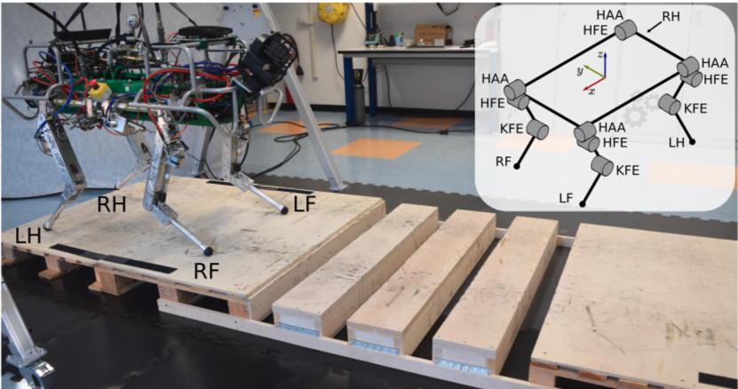
Figure 1: HyQ robot positioned on the terrain template used for experimental test. The naming conventions for the robot joints, axes and legs are seen in the top-right image. The legs are identified as LF (left-front), RF (right-front), LH (left-hind) and RH (right-hind). The leg joints are identified as HAA (hip adduction-abduction), HFE (hip flexion-extension) and KFE (knee flexion-extension).

Our strategy does not rely on visual information only, but rather acts as an interface for the reactive layer of our locomotion controller [3]. The idea is to enhance such controller with reliable feedback obtained from exteroceptive sensing, to increase the traversability of difficult environments. Preliminary simulation results of the strategy here proposed were presented in the short workshop paper [14].

The contributions of this paper are summarized as follows:

1. To the best of our knowledge, the proposed approach is the first to achieve reactive and real-time obstacle negotiation for dynamic gait locomotion, with full on-board computation (control, state estimation and mapping). The fast speed of computation and execution allows the robot to adapt the foot trajectory continuously during the swing motion of the legs, and grants the robot the capability to react favorably against disturbances applied on the trunk at any given time;

2. We improved our previous work [13] in terms of autonomy of training. We replaced the human expert with a heuristic algorithm that generates the ground truth from the terrain morphology, kinematic configurations, foot and leg collisions. This makes the approach self-supervised, and allows to generate more (potentially unlimited) training samples (3300 in [13] vs. 17844 in this work). We also increased the possible outputs (landing positions) from 9 in [13] to 225;

3. We improved the prediction model with respect to [13] by replacing the logistic classifier with a Convolutional Neural Network (CNN), allowing for more complex inputs (i.e., more difficult obstacles) to be processed successfully. To the best of our knowledge, this is the first time a CNN is used to learn foothold corrections in legged locomotion. CNNs are very effective for image processing [15, 16], and are here efficiently implemented to incorporate the knowledge of an effective (yet computationally expensive) heuristic algorithm. This is achieved through low-dimensional parameterization and a carefully balanced network architecture.

The remainder of this paper is organized as follows: Section II summarizes the work related to our proposed strategy; Section III provides a description of the HyQ platform used to test the proposed strategy; Section IV describes the methods to select a safe foothold; simulation and experimental results are shown in Section V; finally, the conclusions and future work are presented in Section VI.

II Related Work

Kolter et al. [17] have provided one of the first applications of terrain awareness to enhance the traversing capabilities of a quadruped robot. To do so, collision probability maps and heightmaps collected a priori are used to train a Hierarchical Apprenticeship Learning algorithm, to select the best footholds in accordance to an expert user.

A similar approach was taken by Kalakrishnan et al. [9]. In contrast to [17], visual feedback was discretized using templates, i.e., portions of terrain in the vicinity of a foothold. With a learning regression method based on expert user selection, a target foothold is associated to each template. The authors have incorporated the classification algorithm into a locomotion planner and demonstrated its validity on the robot LittleDog, traversing highly unstructured terrains.

Both approaches have proved to be powerful, but they rely on external motion capture systems, reducing their field of application to controlled and calibrated environments. In contrast, Belter  et al. [18] used an on-board laser scanner to collect an elevation map of the terrain. Their method searches for useful clues related to the foothold placement, and selects the ones with minimal slippage. The optimal footholds are learned in an unsupervised fashion, inside a simulated environment.

Despite their ability to perform locomotion tasks with on-board sensors only, most of the vision-based foothold selection strategies involve slow motions, mainly to provide enough time to complete the most costly operations such as image processing and optimization. An exception was shown by Wahrmann et al. [19], where the acquisition of swept-sphere-volumes allowed the biped robot Lola to avoid obstacles while moving, with no prior information about the environment. Nevertheless, this strategy was mainly demonstrated for single obstacle avoidance and self collision, and not for rough terrain.

Our previous work [13] is similar to the template-based foothold correction of [9], but it differs due to its implementation in a fully reactive fashion. Heightmaps around the nominal footholds are evaluated to generate continuous motion corrections for the Reactive Controller Framework (RCF) [3]. The corrections are learned from expert demonstration using a Logistic Regression classifier.

More recently, Fankhauser  et al. [12] presented a perception-based statically stable motion planner for the quadruped robot ANYmal. For each footstep, the algorithm generates a foothold (upon rejection of unsafe and kinematically unfeasible solutions), a collision free foot trajectory, and a body pose. The work here presented differs from this because it can deal with dynamic gaits (e.g., a trotting gait), it accounts for the leg collisions when generating collision-free trajectories for the foot, and it can deal with external disturbances during the whole locomotion stride.

III System Overview

The quadruped robot HyQ [20] (Fig. 1) is a hydraulically actuated, versatile research platform. It weighs $90\text{\,}\mathrm{kg}$, is $1\text{\,}\mathrm{m}$ long and $1\text{\,}\mathrm{m}$ tall. Each leg has 3 Degrees-of-Freedom (DoF): a Hip joint for Abduction/Adduction (HAA, actuated by a rotary hydraulic motor), a Hip joint for Flexion/Extension (HFE), and a Knee joint for Flexion/Extension (KFE). The latter two joints are actuated by hydraulic cylinders.

Sensors

HyQ is equipped with a variety of proprioceptive sensors (for a detailed reference, see [21]), including: a tactical-grade IMU (KVH 1775), 8 loadcells (located in all the HFE and KFE joints) and 4 torque sensors (located at the motors of the HAA joints). Each joint’s position is measured with a high-resolution optical encoder. These sensors are synchronized by the EtherCAT network, with a maximum latency of $1\text{\,}\mathrm{ms}$.

Exteroceptive sensors include: an ASUS Xtion RGB-D sensor for mapping; a Multisense SL for pose estimation (Visual Odometry (VO) and LiDAR scan matching). The main sensor characteristics are summarized in [5].

Hardware/Software architecture

HyQ is equipped with a Control-PC, running a real-time Linux kernel, and a Vision-PC, running a regular Linux kernel. The two computers are synchronized by means of an NTP server. The first computer executes the robot control commands in a real-time environment, as well as the Extended Kalman Filter state estimator in a non-real-time thread. The Vision-PC collects the exteroceptive inputs, computes the visual odometry and ICP-based scan matching (as described in [5]), and delivers to the Control-PC an elevation map surrounding the robot (see Fig. 2). In case of failure of the Vision-PC, the controller would still be able to operate blindly with a smooth but drifting pose estimate.

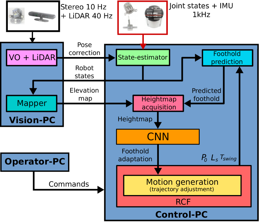
Figure 2: Schematic drawing of our software architecture. The proprioceptive core of the state estimator (green box) runs on the Control-PC, while the low frequency updates from Visual Odometry and LiDAR scan matching are received from the Vision-PC (see [5]). The foothold prediction, the heightmap acquisition and the CNN-based foothold adaptation are executed inside the Control-PC. The CNN sends the adaptation commands to the RCF motion generation module.

IV Visual Foothold Adaptation for Locomotion

In this section, we explain our strategy to deal with computationally demanding visual information. We seek to embed domain knowledge from legged locomotion into a CNN-based learning algorithm. This strategy is primarily applied to the trotting motions from the RCF [3]. For the sake of generality, we have also applied our strategy to the haptic crawl of [1]. The key elements of our strategy are: 1. prediction of the next foothold for each leg; 2. acquisition of heightmap information in the vicinity of the next foothold; 3. foothold evaluation based on kinematics and terrain roughness; 4. training and learning based on a CNN; 5. feet trajectory adjustment for foothold adaptation. These elements are explained in detail next.

IV-A Prediction of the nominal foothold

With foothold prediction we indicate the estimation of the landing position of a foot during the leg’s swing phase. This quantity, expressed in the world frame, is hereafter defined as nominal foothold. The computation of a nominal foothold differs significantly depending on the motion of the trunk.

Some crawl gait implementations do not move the trunk during the swing phase motion of the legs (e.g., our haptic crawl [1]). The nominal foothold can be computed at lift-off according to the desired direction of motion. Therefore, the only source of error between the nominal and the actual foothold comes from foot trajectory tracking.

On the other hand, in gaits that yield motion of the trunk during swing phase (e.g., a diagonal trot), the nominal foothold has to account for the trunk velocity in addition to the foot trajectory tracking. Hence there are two sources of uncertainty: trajectory tracking and trunk state estimation (position and velocity).

In the RCF, the foot swing trajectory is described by a half ellipse, where the major axis corresponds to the step length. To compute the nominal foothold, we use the following approximation:

$$P_{n}=P_{0}+\frac{L_{s}}{2}+(T_{swing}-t_{swing})\dot{X}_{b},$$ (1)

where $P_{n}$ is the nominal foothold position in world coordinates, $P_{0}$ is the position of the center of the ellipse at lift-off in world coordinates, $L_{s}$ is the step length vector, $T_{swing}$ is the swing period (defined by the duty factor $D_{f}$ and the step frequency $f_{s}$), $t_{swing}$ is the time elapsed from the latest lift-off event to the touchdown event, and $\dot{X}_{b}$ is the trunk velocity. Intuitively, the second term on the right hand side of (1) is the distance covered by the leg due to the leg trajectory execution, while the third term is the distance travelled by the trunk, assuming that $\dot{X}_{b}$ is constant over the rest of the swing phase $T_{swing}-t_{swing}$.

In (1), $P_{0}$ and $\dot{X}_{b}$ are taken from the state estimator and are therefore affected by uncertainty (see [5]). To understand the effects of this uncertainty, we conducted a series of preliminary experiments with the robot trotting on flat terrain. A comparison between the actual foot landing position and the predicted one along the swing phase from (1) showed an average error of approximately $3\text{\,}\mathrm{cm}$.

IV-B Foothold heightmap

We define as foothold heightmap (or simply heightmap) a squared, bidimensional and discrete representation of the terrain where each pixel describes the height of a certain area. The heightmap is obtained considering its center as the nominal foothold and oriented with respect to the Horizontal Frame of the robot, which is a frame whose origin coincides with the body frame, with the $xy$ plane always perpendicular to the gravity vector (for a detailed explanation of the Horizontal Frame, see [3]). Since we are considering robots with point-feet, we define the foothold as a 3-D space position.

Given a nominal foothold, the heightmap around it can be easily extracted from the elevation map computed on-board by the Vision-PC (see Section III). We obtain this elevation map using the Grid Map interface from [22]. The heightmap is then analysed to adapt the landing position of the feet and avoid unsafe motions (see Section IV-C).

The heightmap is parametrized by size and resolution. These two parameters are depicted in 3. Both parameters are the result of a compromise between computational expense and task requirements. We want to avoid processing large amounts of data, while retaining a level of detail that is meaningful for the given task. A detailed discussion on appropriate parameter selection can be found in [13]. Fig. 3 shows an example of a heightmap. Each pixel of the image corresponds to a possible foothold.

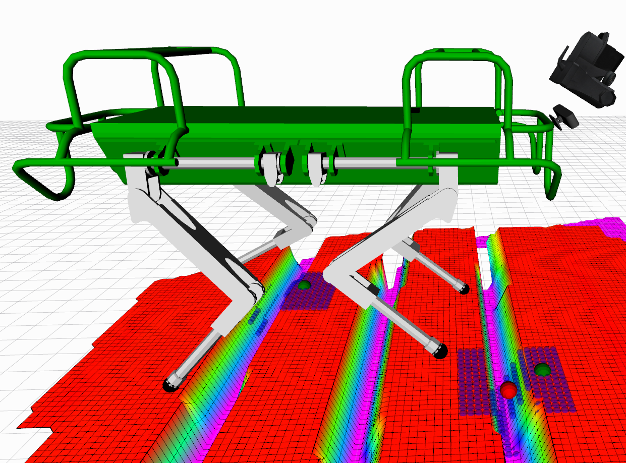
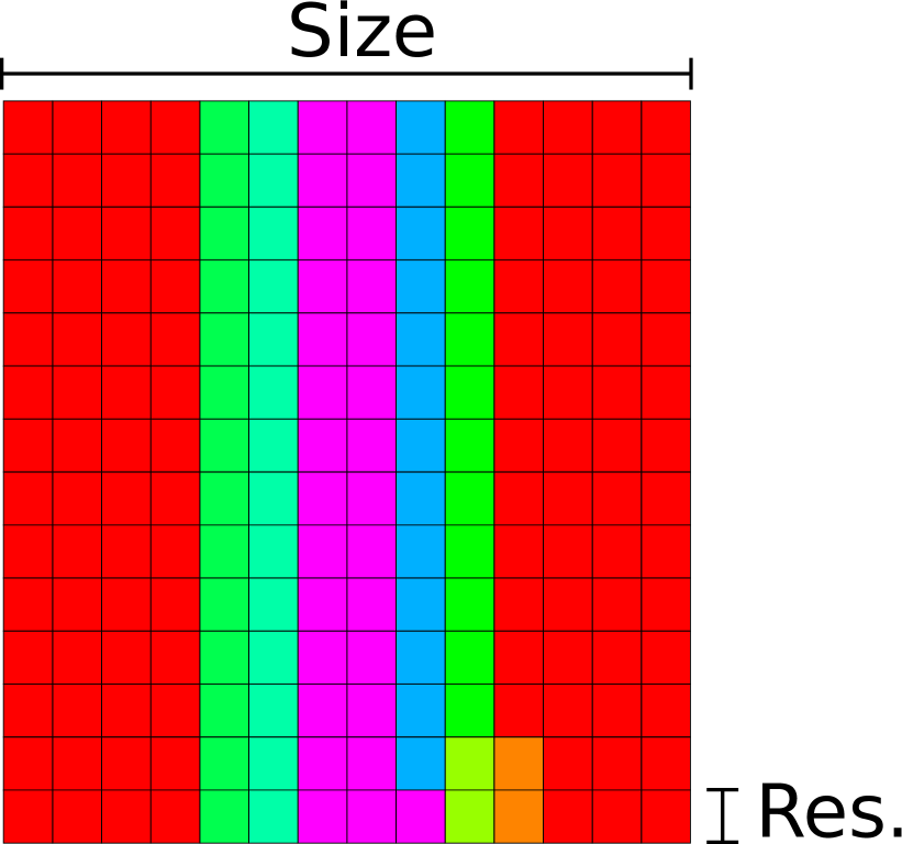
Figure 3: Simulation of HyQ trotting while acquiring an elevation map of the terrain (represented in false colors) using the RGB-D sensor (left). The heightmaps used as inputs to the neural network are shown as squares comprised by the blue spheres, where each sphere is a potential foothold. The nominal foothold is represented by the red sphere, while the corrected foothold is represented by the green sphere. On the right, the heightmap corresponding to the right front leg is shown in false colors. Size and resolution are also indicated. The dark red intensities correspond to the maximum height values, whereas the dark magenta intensities correspond to the minimum ones.

When dimensioning the heightmap, we would like to avoid blind spots (i.e., empty areas between two consecutive foothold heightmaps). We opt for $30\times 30$ $\text{\,}\mathrm{cm}$ heightmap size, with a resolution of $2\text{\,}{\mathrm{cm}}^{2}$ for each pixel (heightmap of $15\times 15$ pixels).

Since drift-free and real-time mapping is still an open issue for dynamic motions, we analyze the degree of uncertainty coming from the map and consider a safety margin to avoid dangerous drifted map locations (see Section IV-C).

IV-C Foothold Adaptation Heuristic Criteria

In this section, we describe the heuristic algorithm used to train automatically the CNN (described in Section IV-D). The algorithm evaluates each foothold inside the heightmap according to the following criteria:

Kinematics

if a foothold is outside the workspace of the robot leg, the pixel is discarded.

Terrain Roughness

for each heightmap pixel, we compute the mean and the standard deviation of the slope relative to its neighborhood. We define a specific threshold for the sum of the standard deviation and the mean of the slope, according to the foot radius. The footholds with values above this threshold are discarded.

Uncertainty Margin

to account for uncertainty, footholds within a certain radius that are deemed as unsafe according to the terrain roughness, are discarded. This also implicitly prevents from stepping close to obstacle edges.

We experimentally identified an uncertainty of $3\text{\,}\mathrm{cm}$ around a nominal foothold, related to errors in the foothold prediction due to the trunk state estimation. In addition, a short term map drift of $2.5\text{\,}\mathrm{cm}$ (mainly due to pose estimation drift) has also been observed after traversing a distance of approximately $2\text{\,}\mathrm{m}$.

Frontal Collision

for each pixel, we evaluate potential foot frontal collisions along the corresponding trajectory from the lift-off location. In Fig. 4, the pixels marked with a red ✖ symbol correspond to discarded footholds, due to frontal collisions.

Leg Collision

similarly to frontal collisions, we evaluate the intersection between the terrain and both leg limbs throughout the whole step cycle (i.e., stance and swing phases). The discarded footholds due to leg collision are shown in Fig. 4 with a light brown ✖.

Distance to nominal foothold

given all valid footholds upon evaluation of the previous criteria, the algorithm chooses as optimal the one closest to the nominal foothold. This minimizes the deviation from the original trajectory.

Let $x\in\mathbb{R}^{n\times n}$ be an input heightmap. We denote $g_{i}(x):\mathbb{R}^{n\times n}\to\mathbb{Z}_{2}^{n\times n}$ as a mapping that takes a heightmap $x$ as input and outputs a matrix of binary values indicating the elements in $x$ that correspond to safe footholds according to one of the previous criteria. We define four mappings $g_{k}$, $g_{t}$, $g_{f}$ and $g_{l}$, corresponding to: kinematics; terrain roughness and uncertainty margin; frontal collision; and leg collision, respectively. A feasible foothold is defined as a foothold that is deemed as safe according to all four mappings. Furthermore, we define $g(x)$ as

$$g(x)=g_{k}(x)\wedge g_{t}(x)\wedge g_{f}(x)\wedge g_{l}(x),$$ (2)

where the operator $\wedge$ represents a coefficient-wise logical AND. The elements that are equal to $1$ of the matrix coming out of $g(x)$ correspond to feasible footholds. The heuristic mapping $h:\mathbb{R}^{n\times n}\to\{0,1\}^{m}$, computes the feasible footholds according to $g(x)$ and outputs a “one-hot vector” that represents the optimal landing point, as the one with the smallest Euclidean distance to the nominal foothold.

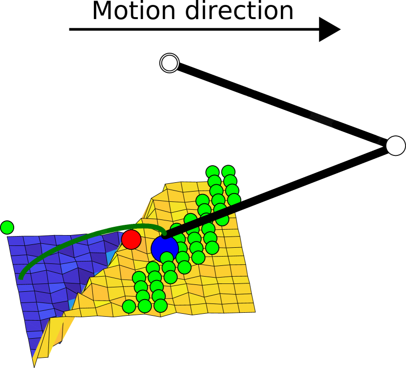
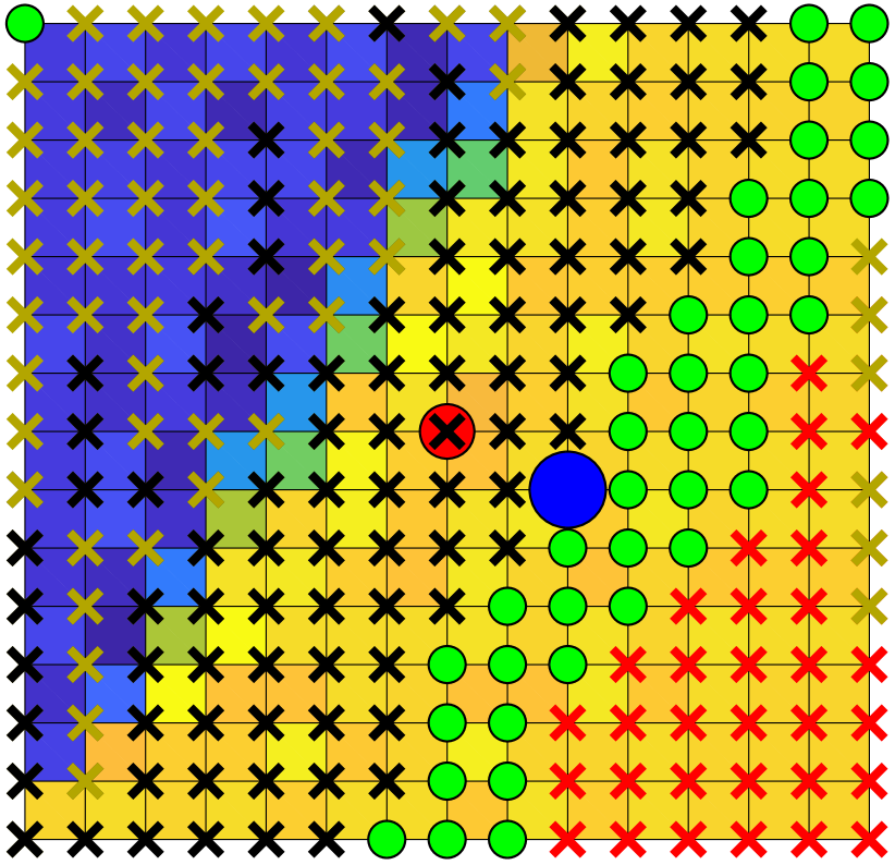
Figure 4: Example of evaluated foothold heightmap. The left image shows a hind leg and the adapted trajectory. The solid black lines are the upper and lower limbs of the leg and the dark green solid line represents the foot trajectory. The red sphere is the nominal foothold, the green spheres are feasible footholds, and the blue one is the optimal according to the heuristics. A top view of the same heightmap is shown on the right. In addition to the feasible footholds, crosses correspond to the discarded footholds due to: the uncertainty margin and terrain roughness (black), foot frontal collision (red) and shin collision (light brown).

Fig. 4 shows the feasible footholds as green spheres, and the optimal foothold with a blue sphere.

IV-D CNN Training

We decided to use a CNN as model for predicting the outputs of the heuristics, since it has better predictive capabilities (yet low computational requirements) than the Logistic Regressor we used in [13]. Our input to the CNN are matrices of $15\times 15$ corresponding to foothold heightmaps. As output, we obtain a foothold corresponding to one of the labelled pixels that represent a landing position, as depicted in the right image of Fig. 4.

To generate the training set, heightmaps can be obtained from three different data sources: simulation, artificial generation or experiments. In this paper, we only use simulated and artificially generated data. Simulated data refers to heightmaps collected from our simulation environment in Gazebo, including sensors and the robot dynamics. Artificial data corresponds to heightmaps generated with no physical or sensor data coming from simulation. We define the elements of the $15\times 15$ matrices in MATLAB to represent bars, gaps and steps of different lengths, heights and at various orientations.

Let again $x\in\mathbb{R}^{n\times n}$ be an input heightmap. Note that in our setting $n=15$. We denote by $f_{w}:\mathbb{R}^{n\times n}\to[0,1]^{m}$ the CNN classifier parametrized by a weight vector $w\in\mathbb{R}^{d}$, where $d=8238$ (number of parameters of the CNN) and $m=226$ (number of potential footholds). Using the heuristic mapping $h(x)$ outlined in Section IV-C, we build a dataset of $N$ labeled examples $D=(x_{i},h(x_{i}))_{i=1}^{N}$ from simulated and artificially generated data. To improve the robustness against noisy heightmaps, the training set is corrupted by zero-mean Gaussian noise with a standard deviation of $3\text{\,}\mathrm{cm}$.

The network is trained to minimize the cross-entropy loss on $D$. Namely, we approximately solve the following optimization problem

$$\min_{w}-\frac{1}{N}\sum_{i=1}^{N}h(x_{i})\circ\log f_{w}(x_{i}),$$ (3)

by stochastic gradient descent, where $\circ$ denotes element-wise product.

To choose the architecture of the CNN, we used the same training set as in [13]. We started from a standard architecture (similar to LeNet [23]) and decreased the size of the CNN as much as possible, without compromising the validation accuracy (which was nearly 100%). After increasing the size of the training set, 99% of the predictions of the CNN were feasible footholds (see Equation (2)), from which 76% of the time the prediction was optimal. These prediction results are summarized in Section V-A. We came to the conclusion that the architecture depicted in Fig. 5 is suitable for our application. Highly accurate predictions are not needed as long as the selected foothold is safe according to the heuristics (see Table I).

A comparison between the CNN and the heuristic algorithm in terms of performance and computational time is also detailed in Section V-A.

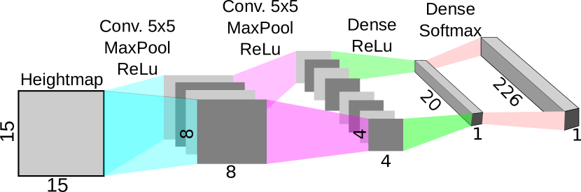
Figure 5: Architecture of the convolutional neural network. The input is a $15\times 15$ matrix corresponding to a heightmap around the vicinity of a foothold. There are 2 convolutional layers, the first one performs convolution of the heightmap with 4 kernels and the second takes the output of the first layer and performs convolution with $8\times 4$ kernels. Both convolutions are performed to retain the input size with the appropriate zero-padding and all kernels are $5\times 5$. Max-pooling is used in both layers to downsample the data, providing feature maps of $8\times 8$ for the first layer and $4\times 4$ for the second layer. The activation function is the Rectified Linear Unit (ReLu).

IV-E Adjustment of the Foot Swing Trajectory

After the CNN has been trained, it can infer a foothold adaptation from a previously unseen heightmap sample. The difference between the optimal foothold and the nominal one is sent to the trajectory generator module as a relative displacement to adapt the original foot swing trajectory.

To avoid aggressive control actions, the foothold corrections are collected from the lift-off to the trajectory apex only. Then, the controller tracks the latest adjusted trajectory available before the apex.

V Results

In this section we present the results regarding the computational performance and the locomotion robustness we achieved with the proposed strategy, both in simulation and experiments.

V-A CNN Prediction Results

We compared the time required to compute a foothold adaptation from the same heightmap for both the heuristic algorithm and the CNN. As a metric for comparison, we use the number of clock tick counts between the beginning and the end of each computation divide by the computer clock frequency. To achieve real-time safe performances, these times should be low on average and display little variance.

To speed up the computation of the heuristics, the algorithm incrementally expands the search radius from the center of the heightmap, i.e., from the nominal foothold, and stops once a feasible foothold is found. In the case of the computation of the full-blown heuristic algorithm, the computational times range from $0.1\text{\,}\mathrm{ms}$ to $20\text{\,}\mathrm{ms}$. The prediction from the CNN takes from $0.072\text{\,}\mathrm{ms}$ to $0.1\text{\,}\mathrm{ms}$. The CNN-based model is therefore 15 to 200 times faster than the heuristic algorithm. Indeed, the computational time increase in a nonlinear fashion along with the complexity of the heightmap, while the neural network presents a computational time less sensitive to the input. Furthermore, the duration of the control loop of our system is $4\text{\,}\mathrm{ms}$, making the computation of the CNN at least 40 times faster than the task rate, allowing to run it in real-time.

In Table I, we summarize the results of the CNN performance when predicting the optimal footholds. From a total number of 35688 examples (for both front and hind legs) we used half dataset as training set and half as testing set. It is worth noting that the percentage of accurate predictions is not notably high (about 76% for both legs). Nevertheless, by looking closely to the false positives, approximately 99% of them were sub-optimal decisions according to the distance criterion, yet deemed as safe with respect to the other criteria (see Section IV-C). This means that, if the foothold is not optimal, the chosen foothold is still safe.

Regarding the quality of predicted footholds with respect to our previous work [13], we initially compared the results of both learning algorithms (CNN vs logistic regression) applied to the same training set used to train the logistic regression classifier, consisting of 3300 examples with 9 possible footholds. The output layer of the CNN was initially set to be $9\times 1$, matching the number of possible footholds. We improved the prediction accuracy to nearly a 100% using the CNN-based classifier, compared to a 90% using the logistic regression. This result and the automation of the training process drove us to increase the number of outputs (from 9 to 226). We compared the CNN-based classifier with a logistic regression using 226 possible outputs and a much larger number of examples. The CNN classifier proved to have better prediction accuracy (76% vs 68%) and yielded a much lower number of parameters (8238 vs 51076).

TABLE I: Results of prediction coming from the neural network on the test set.

Leg	Perfect match	Unsafe footholds	Safe footholds
Front	13718/17844 (76.88%)	47/17844 (0.26 %)	17797/17844 (99.74 %)
Hind	13700/17844 (76.78%)	21/17844 (0.12 %)	17823/17844 (99.88 %)

V-B Simulation and Experimental Results

To assess improvements in terms of locomotion robustness, we created challenging scenarios composed of a series of gaps. These multi-gap terrain templates are built up from short beams ($15\text{\,}\mathrm{cm}$ height and $20\text{\,}\mathrm{cm}$ width), equally spaced by $10\text{\,}\mathrm{cm}$, and pallets ($15\text{\,}\mathrm{cm}$ height). This scenario is used for both simulation and experimental tests: a nine-gap template for the simulated tests (see Fig. 6) and a four-gap template for the experimental ones (see Fig. 1).

In both simulation and experimental tests the locomotion robustness is evaluated while the robot is performing a trotting gait over the beams at different velocities ($0.3\text{\,}\mathrm{m}\text{\,}{\mathrm{s}}^{-1}$ and $0.5\text{\,}\mathrm{m}\text{\,}{\mathrm{s}}^{-1}$) and under external disturbances. The locomotion robustness is evaluated by observing the tracking of the robot desired velocity and trunk height. To evaluate the performance repeatability, we considered the data of 5 trials for each desired velocity. The trotting gait is performed with step frequency of 1.4 Hz, duty factor of 0.65 and a default step height of $12\text{\,}\mathrm{cm}$.

We will end the section with complementary experimental results that show the implementation of our strategy to provide foothold adaptation on a static crawl algorithm [1].

V-B1 Simulation Results

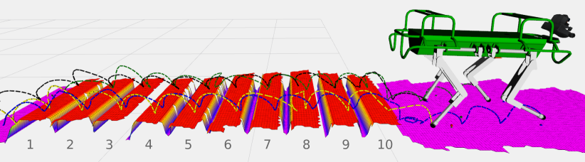
Figure 6: Simulation of gap crossing scenario. Dashed lines correspond to feet trajectories corrected by the vision-based adaptation, during $0.5\text{\,}\mathrm{m}\text{\,}{\mathrm{s}}^{-1}$ trotting gait. The feet trajectories are identified as: left-front (green), right-front (blue), left-hind (black) and right-hind (yellow).

Fig. 6 depicts the details of the simulation scenario showing the elevation map computed by the perception system and the resulting feet trajectories during a multi-gap crossing. Through the footprints (dashed lines) it is possible to see the effect of the foothold adaptation on the original feet trajectories.

Using the beam numbers shown at the bottom of Fig. 6, several examples of corrections that avoided stepping inside the gap can be easily identified: left-front foot double stepping on beam 5 and stepping over beam 6 (green line); right-hind foot stepping over beam 7 and double stepping on beam 8 (yellow line). The right-front foot steps over beam 10 (blue line) to avoid placing the foot too close to the beam edge. The results of the 5 trials of the multi-gap crossing at different velocities are shown in Fig. 7.

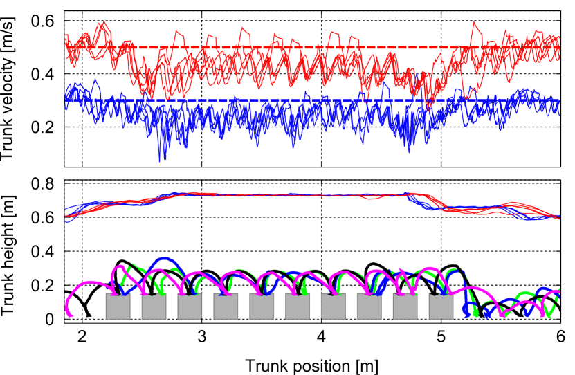
Figure 7: Trotting over multi-gap scenario at different velocites. The top figure shows five simulation trials for $0.3\text{\,}\mathrm{m}\text{\,}{\mathrm{s}}^{-1}$ (blue) and $0.5\text{\,}\mathrm{m}\text{\,}{\mathrm{s}}^{-1}$ (red) trot. Dashed lines represent desired crossing velocity. The bottom figure shows the trunk height while crossing, the position of the beams and one example of the resulting feet trajectories for one of the trials performed at $0.5\text{\,}\mathrm{m}\text{\,}{\mathrm{s}}^{-1}$.

As a last simulation example, we test the capabilities of our strategy to respond against external perturbations and show the benefits of having a continuous adaptation. During the same gap-crossing task shown before, with a $0.3\text{\,}\mathrm{m}\text{\,}{\mathrm{s}}^{-1}$ trotting, we apply a series of perturbations of $500\text{\,}\mathrm{N}$ every $2\text{\,}\mathrm{s}$ with a duration of $0.1\text{\,}\mathrm{s}$ each. The perturbations are applied on the base longitudinal direction disturbing the forward motion. Two cases are studied in this setup: the first corresponds to the case when the adaptation is only computed at the lift-off, and the trajectory is not corrected during the swing phase (red lines in Fig. 8); in the second case, the foothold adaptation is continuously computed and can be modified along the swing phase (blue lines in Fig. 8). It can be seen that in some cases, when the adaptation is only computed at the lift-off, the velocity of the trunk decreases considerably and the trunk height is less stable. Such tracking errors, caused by undesired impacts with the beams, happen due to the lack of foothold adaptation during the swing phase.

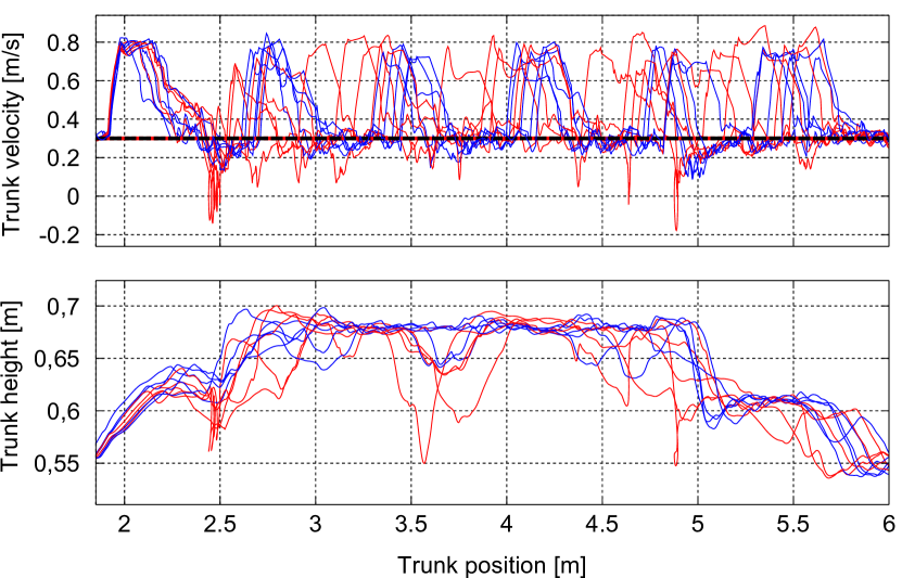
Figure 8: Variation of velocity with $0.1\text{\,}\mathrm{s}$ force disturbance of $500\text{\,}\mathrm{N}$ every $2\text{\,}\mathrm{s}$ and the trunk height while crossing multiple gaps for several simulation trials. The blue lines represent the trials performed with the correction set to be executed continuously during swing. The red lines show the trials where the correction is computed only once at the lift-off for each leg.

V-B2 Experimental results

we prepared the setup depicted in Fig. 1 for the gap-crossing experiments. To show how challenging this task can be for a blind robot, we also present the results of 5 trials using the RCF without the foothold adaptation. The results of these trials are shown in Fig. 9.

As it can be seen, the robot was not able to complete the task without the visual-based adaptation. With visual foothold adaptation the goal was achieved with similar performances between the $0.3\text{\,}\mathrm{m}\text{\,}{\mathrm{s}}^{-1}$ and $0.5\text{\,}\mathrm{m}\text{\,}{\mathrm{s}}^{-1}$ trials. The resulting feet trajectories of one of the trials at $0.5\text{\,}\mathrm{m}\text{\,}{\mathrm{s}}^{-1}$ can also be seen at the bottom part of Fig. 9.

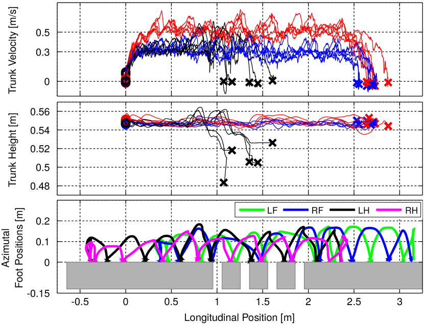
Figure 9: Experimental trotting over gaps, for different desired trunk forward velocities, with and without visual feedback. The two top plots correspond to trials at $0.3\text{\,}\mathrm{m}\text{\,}{\mathrm{s}}^{-1}$ (blue), $0.5\text{\,}\mathrm{m}\text{\,}{\mathrm{s}}^{-1}$ (red) with visual feedback. Black lines show trials at $0.3\text{\,}\mathrm{m}\text{\,}{\mathrm{s}}^{-1}$ without visual feedback. Five trials are shown for each of the cases. Circle and cross markers indicate the beginning and the end, respectively, of each corresponding trajectory. The bottom plot shows the position of the beams and the resulting feet trajectories for one of the trials performed at $0.5\text{\,}\mathrm{m}\text{\,}{\mathrm{s}}^{-1}$.

The robustness of the robot against external disturbances was also experimentally tested on top of the multi-gap terrain template. For such test, we placed the robot on top of one of the pallets, displayed on the bottom-left in Fig. 10, and commanded the robot to keep its position on it while trotting. Then, we disturbed the robot by pulling it and forcing it to go repeatedly over the gaps. Fig. 10 shows video screenshots of disturbance experiments where the robot is subject to strong pulling forces (estimated to be around $500\text{\,}\mathrm{N}$). It can also be observed that the robot is able to keep its balance and to come back to its commanded position without stepping inside the first gap. It is worth highlighting the robust autonomy of the closed-loop system, since the robot is only commanded to keep its global position and no base trajectory is pre-designed while it is disturbed.

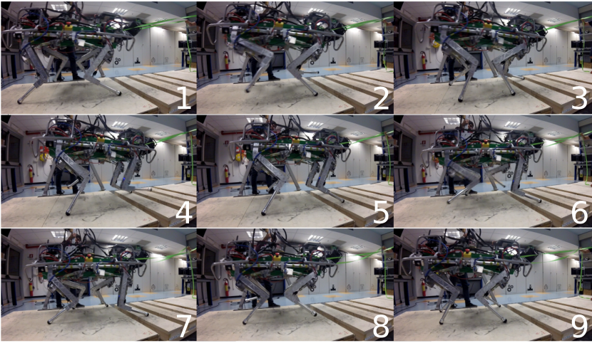
Figure 10: Video screenshots of the disturbance test showing the robot reactions while being pulled towards the gaps.

As complementary result, we show the generality of the proposed strategy by implementing it into a blind static crawl algorithm [1]. In the case of the crawl, we created a gap-crossing scenario where the robot has to step on a series of wooden beams to then take a step down and reach the ground. For this task, the robot is commanded to go forward with a velocity of $0.1\text{\,}\mathrm{m}\text{\,}{\mathrm{s}}^{-1}$. We compare the results between the haptic blind crawling strategy and enhanced with the CNN-based foothold adaptation. In the case of a static crawl the nominal footholds are already provided in the world frame and do not need to be predicted. Therefore, we compute the correction only at lift-off and execute the trajectory without changing it during the swing phase. It can be seen in the series of snapshots in Fig. 11, and in the attached video, that the robot succeeded in crossing the scenario when the CNN-based foothold adaptation is implemented. The robot was not able to cross the gaps without foothold adaptation.

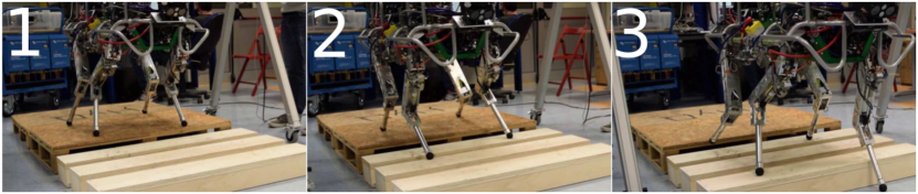
Figure 11: Video screenshots of a crawl experiment showing the robot crossing a series of gaps.

VI Conclusions

We have presented a novel strategy for continuous foothold adaptation based on a Convolutional Neural Network. We evaluated the performance of the approach by performing dynamic trotting and static crawling gaits on a challenging surface, difficult to traverse if only proprioceptive sensors and haptics are used. The various simulated and experimental trials, at different forward velocities and under external disturbances, demonstrated the robustness of the strategy and its repeatability. Moreover, we showed that the proposed strategy is more robust with respect to the ones that only adapt the nominal foothold at the leg lift-off.

The CNN resulted to be up to 200 times faster than computing the full-blown heuristics to find a safe foothold, showing that the strategy has potential to deal with more complex heuristics and still satisfy the real-time constraints. Due to the low computational load of the method (40 times faster than the task rate), our future work will concentrate on learning more complex heuristics that evaluate footholds in a two-step horizon, dynamic criteria for better robot balancing, posture adjustment and gait parameter modulation. Moreover, we will customize even further the CNN architecture to better reflect the computations performed by the heuristics.

References

- [1] M. Focchi, A. del Prete, I. Havoutis, R. Featherstone, D. G. Caldwell, and C. Semini, “High-slope terrain locomotion for torque-controlled quadruped robots,” Autonomous Robots, vol. 41, no. 1, Jan 2017.
- [2] R. Hodoshima, T. Doi, Y. Fukuda, S. Hirose, T. Okamoto, and J. Mori, “Development of TITAN XI: a quadruped walking robot to work on slopes,” in IEEE/RSJ International Conference on Intelligent Robots and Systems (IROS), Sep 2004.
- [3] V. Barasuol, J. Buchli, C. Semini, M. Frigerio, E. R. D. Pieri, and D. G. Caldwell, “A reactive controller framework for quadrupedal locomotion on challenging terrain,” in IEEE International Conference on Robotics and Automation (ICRA), May 2013.
- [4] H.-W. Park, P. M. Wensing, and S. Kim, “High-speed bounding with the MIT Cheetah 2: Control design and experiments,” The International Journal of Robotics Research, vol. 36, no. 2, Mar 2017.
- [5] S. Nobili, M. Camurri, V. Barasuol, M. Focchi, D. G. Caldwell, C. Semini, and M. Fallon, “Heterogeneous Sensor Fusion for Accurate State Estimation of Dynamic Legged Robots,” in Proceedings of Robotics: Science and Systems (RSS), Jul 2017.
- [6] C. Mastalli, A. Winkler, I. Havoutis, D. G. Caldwell, and C. Semini, “On-line and On-board Planning and Perception for Quadrupedal Locomotion,” in IEEE International Conference on Technologies for Practical Robot Applications (TEPRA), May 2015.
- [7] P. Fankhauser, M. Bloesch, C. Gehring, M. Hutter, and R. Siegwart, “Robot-centric elevation mapping with uncertainty estimates,” in International Conference on Climbing and Walking Robots (CLAWAR), Apr 2014.
- [8] M. Camurri, S. Bazeille, D. G. Caldwell, and C. Semini, “Real-time depth and inertial fusion for local SLAM on dynamic legged robots,” in IEEE International Conference on Multisensor Fusion and Integration for Intelligent Systems (MFI), Sep 2015.
- [9] M. Kalakrishnan, J. Buchli, P. Pastor, and S. Schaal, “Learning locomotion over rough terrain using terrain templates,” in IEEE/RSJ International Conference on Intelligent Robots and Systems (IROS), Oct 2009.
- [10] B. Aceituno-Cabezas, C. Mastalli, H. Dai, M. Focchi, A. Radulescu, D. G. Caldwell, J. Cappelletto, J. C. Grieco, G. Fernandez-Lopez, and C. Semini, “Simultaneous Contact, Gait, and Motion Planning for Robust Multilegged Locomotion via Mixed-Integer Convex Optimization,” IEEE Robotics and Automation Letters, vol. 3, no. 3, Jul 2018.
- [11] M. Wermelinger, P. Fankhauser, R. Diethelm, P. Krüsi, R. Siegwart, and M. Hutter, “Navigation planning for legged robots in challenging terrain,” in IEEE/RSJ International Conference on Intelligent Robots and Systems (IROS), Oct 2016.
- [12] P. Fankhauser, M. Bjelonic, C. D. Bellicoso, T. Miki, and M. Hutter, “Robust Rough-Terrain Locomotion with a Quadrupedal Robot,” in IEEE International Conference on Robotics and Automation (ICRA), May 2018.
- [13] V. Barasuol, M. Camurri, S. Bazeille, D. Caldwell, and C. Semini, “Reactive Trotting with Foot Placement Corrections through Visual Pattern Classification,” in IEEE/RSJ International Conference on Intelligent Robots and Systems (IROS), Oct 2015.
- [14] O. Villarreal, V. Barasuol, M. Camurri, M. Focchi, L. Franceschi, M. Pontil, D. G. Caldwell, and C. Semini, “Deep Convolutional Terrain Assessment for Visual Reactive Footstep Correction on Dynamic Legged Robots,” in IROS 2018 Workshop: Machine Learning in Robot Motion Planning, Oct 2018.
- [15] A. Krizhevsky, I. Sutskever, and G. E. Hinton, “ImageNet Classification with Deep Convolutional Neural Networks,” in International Conference on Neural Information Processing Systems (NIPS), Dec 2012.
- [16] I. Goodfellow, Y. Bengio, and A. Courville, Deep Learning. MIT Press, 2016, http://www.deeplearningbook.org.
- [17] J. Z. Kolter, M. P. Rodgers, and A. Y. Ng, “A control architecture for quadruped locomotion over rough terrain,” in IEEE International Conference on Robotics and Automation (ICRA), May 2008.
- [18] D. Belter and P. Skrzypczyński, “Rough terrain mapping and classification for foothold selection in a walking robot,” Journal of Field Robotics, vol. 28, no. 4, Jul 2011.
- [19] D. Wahrmann, A. C. Hildebrandt, R. Wittmann, F. Sygulla, D. Rixen, and T. Buschmann, “Fast object approximation for real-time 3D obstacle avoidance with biped robots,” in IEEE International Conference on Advanced Intelligent Mechatronics (AIM), Jul 2016.
- [20] C. Semini, N. G. Tsagarakis, E. Guglielmino, M. Focchi, F. Cannella, and D. G. Caldwell, “Design of HyQ - a Hydraulically and Electrically Actuated Quadruped Robot,” Journal of Systems and Control Engineering, vol. 225, no. 6, Aug 2011.
- [21] M. Camurri, “Multisensory State Estimation and Mapping on Dynamic Legged Robots,” Ph.D. dissertation, Istituto Italiano di Tecnologia and University of Genoa, Apr 2017.
- [22] P. Fankhauser and M. Hutter, “A Universal Grid Map Library: Implementation and Use Case for Rough Terrain Navigation,” in Robot Operating System (ROS) - The Complete Reference (Volume 1), A. Koubaa, Ed. Springer, Feb 2016, ch. 5.
- [23] Y. Lecun, L. Bottou, Y. Bengio, and P. Haffner, “Gradient-based learning applied to document recognition,” Proceedings of the IEEE, vol. 86, no. 11, Nov 1998.