A big data based method for pass rates optimization
in mathematics university lower division courses

Abstract

In this paper a big data based method is presented, for the enhancement of pass rates in mathematical university lower division courses, with several sections. We propose the student-lecturer partnership as the cornerstone of our optimization process. First, the students-lecturer success probabilities are computed using statistical segmentation and profiling techniques in the available historical data. Next, using integer programming models, the method finds the optimal pairing of students and lecturers, in order to maximize the success chances of the students’ body. Finally, the analysis of our method as an economic process, as well as its importance for public universities of the third World, will be presented throughout the paper.

1 Introduction

It is well-known that improving pass rates in mathematics courses is of paramount importance for academic institutions all over the world. This objective becomes even more critical for public universities as they subside partially or totally the education of its enrolled undergraduates; subject to the country’s legislation and the student’s economic stratification.

The general consensus is that creating better conditions for the students will improve students’ success. Hence, most of the work done in order to address this challenge has two principal directions:

1. The traditional pedagogical approach which, essentially aims to improve the presentation of the course contents on two fronts: presentation of mathematical discourse i.e., curricula reform, development of course materials and improvement of the lecturer’s instructional practice. Part of the latter are the teaching evaluations’ open questions, giving feedback to the instructor about how people felt during his/her classes.

2. The uses of technology in the learning of mathematics. One stream goes in the recollection of data and the measurement of the resource impact in the cognitive process: development of LMS platforms and real-time feedback interfaces [1]. The other stream explores the use of the aforementioned harvested information to improve the learning process [2]: targeted problem sets and training tests [3], identification of favorable pedagogical approaches and learning patterns/styles [4], identification of fortitudes and weaknesses, assessment of study exercise vs skills building [4], problem solving approaches, platforms for interaction between students through the learning process [5]. There is also the use of big data to asses learning rather than improve instructional techniques, such as early detection of students at risk [6].

The present work fits in the second category, in this case, the use of big data to define policies enhancing the higher education production [7] and without raising the costs. More specifically, the method will suggest an optimal design of student body/composition to maximize the pass rate chances. The design is driven by favorable teacher-student partnership, rather than peer diversity or a peer interaction criterion (see [8, 9]). A second aspect of the method is that, it is based on the computation of expectations (conditioned to the students’ segmentation) and not on statistical regression (linear or not), as it pursues the construction of a probabilistic model, rather than the construction of a production function (see [8, 10]). In addition, the input database (which is the method’s input), is updated from one academic term to the next, therefore, it seems more adequate to recompute the conditional expectations term-wisely instead of pursuing rigid regression models. Moreover, given the current computational tools and possibilities, once the method is coded as an algorithm, the proposed updating approach will come at zero cost increase. This is the main reason while our method will be presented and explained, mostly in the format of an algorithm.

Our approach starts from data bases of a public university for 15 semesters, between February 2010 and July 2017, containing the information of academic performance and demographics of its population. A first stage of descriptive statistics allows to identify the success factors by correlation. A second stage revisits the historical performance (15 semesters in total), it defines segmentation profiles and then computes the historical efficiency for each of the involved instructors, conditioned to the quantiles of segmentation. Next, it uses integer programming to find the optimal matching of students-instructors in two different ways. A third stage of the method randomizes the involved factors, namely the profile of the group taking the class, the number of Tenured Track instructors, the number of sections (group) in the course and such. This is aimed to produce Monte Carlo simulations and find the expected values of improvement in the long run. The factors are regarded as random variables with probabilistic distributions computed from the empirical knowledge, recorded in the database and each Monte Carlo simulation arises from one random realization of the algorithm.

1.1 Economic Justification

Whether or not public higher education constitutes a public good, is a subject that has been extensively debated in economics (see, e.g, [11] and [12]). On one side, it benefits the whole society by playing a redistributive role, where low income class students can access higher education to improve their future labor perspectives. On the other side, public higher education can be of limited access.. This last feature shows why the classification of public higher education as a public good, is a matter of debate among economists, because a public good must be accessible to all individuals. Such a debate is not the matter of this paper, but it highlights two important properties of public higher education (its redistribution role, and its limited access), which are relevant to understand the contribution of this work.

The Colombian government has implemented different strategies to address the limited access aspect of education, implementing programs like “Familias en Acción”, a welfare program designed to improve school attendance rates among the young; and “Ser Pilo Paga”, a merit-based financial aid program designed to increase the higher education attendance rates among the poorest. Although these strategies have increased the attendance rates in education (as showed by [13] in the case of higher education), a report from the World Bank ([14]) showed that 37 percent of students starting a bachelors’ degree program withdraw from the higher education system (with percentages going as high as 53 percent, when including short-cycle programs). These numbers show that the limited access aspect of public higher education, can not be addressed only by means of increasing the raw coverage. Higher education institutions need strategies to decrease drop out rates, and require mechanisms to help students to improve their pass rates, grades and others.

This paper provides a mechanism–an algorithm- to potentially help higher education institutions to improve such indicators of student welfare (pass rates and grades). Our approach is to understand the University, not only as an agent that provides education, but also as a rational regulator agent, capable to optimally allocate some of its resources for enhancement of social welfare of its students body.

Throughout the paper we will make remarks emphasizing the interpretation and/or importance of the problem from the economic point of view; these remarks will have a pertinent warning for the reader.

1.2 Organization and notation

The paper is organized as follows. In Section 2, we a brief description of the study case setting and its databases. In Section 3 the available historical information is quantified by a process of statistical segmentation and profiling. In Section 4 the two optimization mechanisms are presented, formulated a problems of integer programming and an assessment of the historical behavior is performed, i.e., compute the theoretical outcome should the method would have been applied in the past. In Section 5 we randomize the study case, using the historical records in order to generate random and plausible instances of the study case and apply the optimization method in order to perform Monte Carlo simulations, as well as observing its asymptotic behavior. Finally, Section 6 delivers the conclusions.

We close the introduction describing the mathematical notation. For any natural number $N\in\bm{\mathbbm{N}}$, the symbol $[N]\overset{\textbf{def}}{=}\{1,2,\ldots,N\}$ indicates the set/window of the first $N$ natural numbers. For any set $E$ we denote by $|E|$ its cardinal and $\wp(E)$ its power set. We understand $\Omega$ as a generic finite probability space $\big{(}\Omega,\wp(\Omega),\bm{\mathbbm{P}}\big{)}$ in which all outcomes are equally likely, i.e. the event probability function satisfies $\bm{\mathbbm{P}}(\{\omega\})=|\Omega|^{-1}$ for all $\omega\in\Omega$. In particular for any event $E\subseteq\Omega$ it holds that

$$\bm{\mathbbm{P}}(E)\overset{\textbf{def}}{=}\dfrac{|E|}{|\Omega|}=\dfrac{\text{number of favourable outcomes}}{\text{total number of possible outcomes}}.$$ (1)

A particularly important probability space is $\mathcal{S}_{N}$, where $\mathcal{S}_{N}$ denotes the set of all permutations in $[N]$, its elements will be usually denoted by $\pi,\sigma,\tau$, etc. Random variables will be represented with upright capital letters, namely $\mathrm{X},\mathrm{Y},\mathrm{Z},...$, expectation and variance of such variables with $\mathbbm{E}(\mathrm{X})$ and $\operatorname*{\mathbb{V}\!ar}(\mathrm{X})$ respectively. Vectors (deterministic or random) are indicated with bold letters, namely $\mathbf{p},\mathbf{g},\mathbf{X}...$ etc. Deterministic matrices are represented with capital letters i.e., $A,G,T$.

2 The study case and its databases

In this work our study case is the performance of lower division mathematics courses at Universidad Nacional de Colombia, Sede Medellín (National University of Colombia at Medellín). The Institution is a branch of the National University of Colombia, the best ranked higher education Institution in Colombia; it is divided in five colleges: Architecture, Science, Humanities & Economical Sciences, Agriculture and Engineering (Facultad de Minas). The colleges are divided in schools and/or departments. The University offers 27 undergraduate programs and 85 graduate programs divided in Specializations, MSc and PhD levels, depending on the school/department. Each semester, the University has an average enrollment of 10000 undergraduates and 2000 graduates with graduation rates of 1240 and 900 respectively. The College of Engineering is the most numerous, consequently, the mathematics lower division courses are highly demanded and have a profound impact in the campus’ life; its teaching and evaluation is in charge of the School of Mathematics.

The School of Mathematics is part of the College of Science, it teaches two types of courses: specialization (advanced undergraduate and graduate courses in mathematics) and service (lower division). The latter are: Basic Mathematics (BM, college algebra), Differential Calculus (DC), Integral Calculus (IC), Vector Calculus (VC), Differential Equations (ODE), Vector & Analytic Geometry (VAG), Linear Algebra (LA), Numerical Methods (NM), Discrete Mathematics and Applied Mathematics. The total demand of these courses amounts to an average of 7200 enrollment registrations per semester. The last two courses, Discrete Mathematics and Applied Mathematics have very low an unstable enrollment, therefore, their data are not suitable for statistical analysis and they will be omitted in the following. On the other hand, the remaining courses are ideally suited for big data analysis, due to its massive nature; see Table 1 below.

Year	Semester	DC	IC	VC	VAG	LA	ODE	BM	NM	Total
2010	1	1631	782	381	1089	983	668	848	142	6524
2013	2	1446	1212	549	1187	1103	786	846	326	7455
2016	2	1569	1296	594	1355	1009	1019	1111	284	8237
Mean	Does not apply	1445.9	1122.9	549.8	1146.5	988.7	801.8	905.4	267.5	7228.5

Table 1: Historical Enrollment Sample. The table shows the mean enrollment for each course for the period from 2010-1 to 2017-1, together with a sample of three semesters in that time window.

On a typical semester these courses are divided in sections (between 8 to 22, depending on the enrollment) of sizes ranging from 80 to 140 (because of classroom physical capacities). There is no graded homework but students have problem sheets as well as optional recitation classes. As for the grading scale 5.0 is the maximum, 3.0 is the minimum pass grade and grades contain only one decimal. The evaluation consists in three exams which the students take simultaneously; the activity is executed with the aid of the software packages SiDEx-$\Omega$ and RaPID-$\Omega$ which manage the logistics of the evaluation and proctoring activities, including the organization of the grading stage. More specifically, for fairness and consistency of the grading process a particular problem is graded by one single grader for all the students, i.e., it is a centralized grading process. As a consequence of the institutional policies described above, the data are statistically comparable. Moreover, the paper-based tests administrator SiDEx-$\Omega$ introduces high levels of fraud control, because of its students seating assignment algorithm; this increases even more the reliability of the data.

2.1 The Databases

The University allowed limited access to its data bases for the production of this work. The information was delivered in five separate tables which were merged in one single database using Pandas: the file Assembled_Data.csv which contains 108940 rows, each of them with the following fields

1. Student’s Personal Information: $\bullet$ Year of Birth $\bullet$ e-mail $\bullet$ ID Number $\bullet$ Last Name and Names $\bullet$ Gender

2. Student’s General Academic Information: $\bullet$ University Entrance Year (AA, Academic Age) $\bullet$ Career $\bullet$ Academic Average (GPA)

3. Student’s Academic Information Relative to the Course: $\bullet$ Course $\bullet$ Course Code $\bullet$ Academic Year $\bullet$ Academic Semester $\bullet$ Grade $\bullet$ Completed vs Canceled $\bullet$ Number of Attempts $\bullet$ Number of Cancellations

4. Student’s Administrative Information Relative to the Course: $\bullet$ Section Number $\bullet$ Schedule $\bullet$ Section Capacity $\bullet$ Number of Enrolled Students $\bullet$ Instructor’s ID Number $\bullet$ Instructor’s Name $\bullet$ Tenured vs. Adjoint Instructor

Remark 1 (Meaning of a row).

It is understood that one registration corresponds to one row, for instance if a particular student registers for DC and LA in the same term, one row is created for each registration, repeating all the information listed in items (i) and (ii) above. The same holds when an individual needs to repeat a course because of previous failure or cancellation.

3 Quantification: Variables, Segmentation and Profiling

In the present work we postulate the Lecturer as one of the most important factors of success, more specifically the aim is to attain the optimal Instructor-Student partnership; in this we differ from [8, 9] where its proposed that the class composition should be driven by the peers interaction. To that end, it becomes necessary to profile the students’ population according to its relevant features.

3.1 Determination of the Segmentation Factor

Computing the correlation matrix of the quantitative factors considered in the Assembled_Data.csv; in the table 2 we display the correlation matrix for the Differential Calculus course. From the Grade row it is clear that the most significant factor in the Grade variable is the Academic Average (GPA) followed by the Academic Age (AA) and the Age. However, the impact of the GPA is about four times the impact of AA and the same holds for the Age factor. Moreover, from the GPA row, it is clear that the most significant factor after the Grade are precisely the Academic Age and the Age (the younger the student, the higher the GPA). In addition, for the remaining courses, similar correlation matrices are observed. Hence, we keep the GPA as the only significant quantitative factor in the Grade variable.

Remark 2.

It is important to mention that the impact of the class size in the students’ performance has been subject of extensive discussion without consensus. While [15, 10] report a significant advantage in reducing class sizes, [16] finds no effect. In our particular case Table 2 shows that the Section Capacity is uncorrelated, not only to the Grade variable, but also to the GPA variable. Moreover the Section Capacity is uncorrelated with the Cancellations (drop out) variable.

FACTOR	Section	Age	AA	# Enrolled	Grade	# Cancellations	# Attempts	GPA
	Capacity			Students
Section Capacity	1.0000	-0.0108	0.0570	0.8334	0.0074	0.0003	0.0393	0.0180
Age	-0.0108	1.0000	0.3069	-0.0168	-0.2031	0.0775	0.1384	-0.2082
AA	0.0570	0.3069	1.0000	0.0416	-0.2164	0.1668	0.4294	-0.1667
# Enrolled Students	0.8334	-0.0168	0.0416	1.0000	0.0252	0.0131	-0.0041	0.0325
➙ Grade	0.0074	-0.2031	-0.2164	0.0252	1.0000	-0.1247	-0.0241	$\star$ 0.8207
# Cancellations	0.0003	0.0775	0.1668	0.0131	-0.1247	1.0000	0.3101	-0.0686
# Attempts	0.0393	0.1384	0.4294	-0.0041	-0.0241	0.3101	1.0000	-0.0401
➙ GPA	0.0180	-0.2082	-0.1667	0.0325	$\star$ 0.8207	-0.0686	-0.0401	1.0000

Table 2: Quantitative Factors Correlations Table, Course: Differential Calculus. The table displays the correlation matrix for the variables of interest (Section Capacity, Age, AA, # Enrolled Students, Grade, # Cancellations, # Attemps, GPA).

Two binary variables remain to be analyzed namely Pass/Fail (PF) and Gender. If we generically denote by $X$ the binary variables and by $Y$ a variable of interest, the point-biserial correlation coefficient is given by

$$r_{pb}\overset{\textbf{def}}{=}\frac{M_{1}-M_{0}}{\sigma}\sqrt{\frac{N_{1}\,N_{0}}{N^{2}}}.$$ (2)

Here, the indexes $0,1$ are the values of the binary variable $X$. For $i=0,1$, $M_{i}$ is the mean value of the variable $Y$ for the data points in the group/event $\{X=i\}$, $N_{i}$ denotes the population of each group $\{X=i\}$, $N=N_{1}+N_{0}$ stands for the total population and $\sigma$ indicates the standard deviation of the variable $Y$.

The correlation analysis between the binary Pass/Fail (PF) variable vs the quantitative factors is displayed in Table 3. As in the Grade variable analysis, the most significant factor in the Pass/Fail variable, is the Academic Average (GPA) followed by the Academic Age (AA) and the Age. In this case however, the impact of the GPA is only three times the impact of AA as well as the Age factor. Again, we keep the GPA as the only significant quantitative factor in the Pass/Fail variable.

	DC	IC	VC	VAG	LA	ODE	BM	NM
Section Capacity	0.0058	0.0139	-0.0296	-0.0986	-0.0147	0.0448	-0.0451	0.0840
Age	-0.1757	-0.2554	-0.3048	-0.1879	-0.2444	-0.2555	-0.0892	-0.3333
AA	-0.1783	-0.2855	-0.3012	-0.1550	-0.2230	-0.3841	-0.0209	-0.2731
# Enrolled Students	0.0070	0.0276	0.0172	-0.0410	0.0602	0.1258	-0.0374	0.1916
Grade	0.8072	0.7987	0.7864	0.8145	0.7959	0.7999	0.7988	0.7922
# Cancellations	-0.1129	-0.1397	-0.1420	-0.1299	-0.1178	-0.1647	-0.0096	-0.1489
# Attempts	-0.0988	-0.1635	-0.1683	-0.1374	-0.1399	-0.1577	-0.0054	-0.2065
➙ GPA	0.6062	0.5892	0.5884	0.6445	0.6063	0.5341	0.6125	0.5828

Table 3: Pass/Fail vs Quantitative Factors, Biserial Correlations Table, Course: All. We display the biserial correlations for each of the variables (Section Capacity, Age, AA, # Enrolled Students, Grade, # Cancellations, # Attemps, GPA) compared to the Pass/Fail variable, per course.

Next, the correlation analysis Gender variable vs the Academic Performance Variables, i.e., Grade, GPA and Pass/Fail (PF) is summarized in the table 4 below. Clearly, the Gender variable has negligible incidence in the Academic Performance Variables, with the exception of the GPA for the Basic Mathematics (BM) course case, where females do slightly better. Since this unique correlation phenomenon is not present in the remaining courses, the Gender variable will be neglected from now on. Finally, it is important to stress that, given the binary nature of the Gender and the Pass/Fail (PF) variables, all the correlation coefficients agree i.e., point-biserial, Pearson and Spearman and Kendall.

	DC	IC	VC	VAG	LA	ODE	BM	NM
Grade	0.0545	0.0584	0.0240	-0.0485	0.0154	0.0164	-0.0740	-0.0405
GPA	-0.0425	-0.0441	-0.0419	-0.0766	-0.0343	-0.0824	-0.1159	-0.0663
Pass/Fail (PF)	0.0509	0.0382	0.0166	-0.0373	0.0103	0.0085	-0.0535	-0.0226

Table 4: Gender vs Academic Performance Variables, Course: All. The biserial correlations of each of the variables in (Grade, GPA, Pass/Fail) compared to the Gender variable, is displaye for each course.

From the previous discussion, it is clear that out of the analyzed variables, the GPA is the only one with significant incidence on the academic performance variables Grade and Pass/Fail. Consequently, this will be used as the unique criterion for the segmentation of students’ population. From now on, our analysis will be focused on the Grade Average and the Pass/Fail variables as measures of success, while the GPA will be used for segmentation purposes discussed in Section 3.2. In Table 5, the global averages (from 2010-1 to 2017-1) of these variables for all the service courses are displayed.

	DC	IC	VC	VAG	LA	ODE	BM	NM
Grade	2.6849	2.7829	3.2198	2.8616	3.0233	3.1170	2.8308	3.1893
GPA	3.2213	3.3527	3.4969	3.2386	3.3201	3.4548	3.2696	3.5330
Pass/Fail	0.5010	0.5339	0.7151	0.5901	0.6398	0.6846	0.5441	0.6924
Number of Tries	1.7382	1.9140	1.4996	1.5205	1.5495	1.7710	1.0549	1.4115

Table 5: Academic Performance Variables Average Values, Course: All. The average performance (as captured by the variables Grade, GPA, and Pass/Fail) of students from 2010-1 to 2017-1, is displayed for each course.

3.2 Segmentation Process

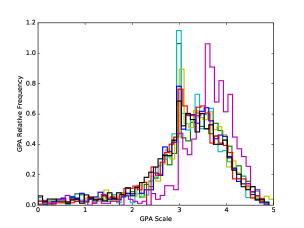
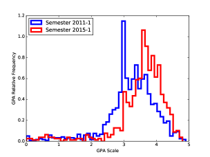
The profiling of students’ population is to be made course-wise. For each group taking a course, the algorithm computes a partition of the interval $[0,5]$ of ten numerical GPA intervals $\big{(}I_{\ell}:\ell\in[10]\big{)}$, so that approximately ten percent of the population is contained in $I_{\ell}$ for all $\ell\in[10]$. Equivalently, if a histogram of relative frequencies is drawn, as in Figure 1, the area between the curve and any interval should be around 0.1. Hence, if $f_{\mathop{}\!\mathit{GPA}}$ is the relative frequency of the $\mathop{}\!\mathit{GPA}$ variable then $\int_{I_{\ell}}f_{\mathop{}\!\mathit{GPA}}\,dx\sim 0.1$ for all $\ell\in[10]$. The process described above is summarized in the pseudocode 1 below.

(a) Example DC. GPA Histogram, Semesters from 2010-1 to 2017-1.

(b) Example DC. GPA Histogram, Semesters 2010-1 and 2015-1.

Figure 1: Differential Calculus GPA Normalized Histogram. Figure (a) Shows the normalized frequencies histograms for all the semesters available in the database Assembled_Data.csv. Figure (b) displays the normalized histogram of only two semesters for optical purposes. Observe that in both cases the area beneath the normalized histogram is exactly equal to one.

Data: Database: Assembled_Data.csv.

Year ($y$) and Semester ($s$).

Analyzed Course: DC, IC, …, NM.

Result: Extremes of the GPA Segmentation Intervals $\big{(}I_{\ell}:\ell\in[L]\big{)}$; extremes = [0, n_1, n_2,…, 5 ]

Initialization;

List_GPA $\leftarrow$ sorted (hash $\mathop{}\!\mathit{GPA}$ variable from

Assembled_Data.csv[(Course = Analyzed Course) & (Year = $y$) & (Semester = $s$ )] ) ;

extremes_0 $\leftarrow$ 0;

for  $i\in[10]$  do

       extremes_i $\leftarrow\big{\lfloor}i\times\frac{\text{length of List\_GPA}}{10}\big{\rfloor}$;

      

end for

if list extremes contains repetitions then

       extremes $\leftarrow$ remove repetitions from extremes

end if

Algorithm 1 Segmentation of Students

Remark 3.

Observe that Algorithm 1 is aimed to produce ten segmentation intervals, however the last instruction considers removing some points out of the eleven extremes previously defined, in case of repetition. Such situation could arise when a particular GPA value is too frequent as it can be seen in Figure 1 (b), for the case of Semester 2011-1, which has a peak at GPA = 3. Similar peaks can be observed in other semesters as Figure 1 (a) shows.

3.3 Computation of the Lecturer’s Performance

The treatment of the lecturer as a success factor is completely tailored to the case of study and it can not be considered as a general method, the expected (average) performance will be computed for the Grade and the Pass/Fail variables. For the computation of instructors’ performance, first a segmentation process $\big{(}I_{\ell}:\ell\in[L]\big{)}$ (as described in Subsection 3.2) has to be done. Next, the computation is subject to the following two principles

1. Adjunct and Tenured (Track or not) lecturers are separated in different groups.

2. If the experience of a particular instructor (the full personal teaching log inside the database Assembled_Data.csv) within a segment $I_{\ell}$ of analysis, accumulates less than 30 individuals, his/her performance within such $I_{\ell}$ is replaced by the average performance of the group he/she belongs to (Adjunct or Tenured) within such group, i.e., the conditional expectation of the Academic Performance Variable ($\mathop{}\!\mathit{APV}$) subject to the segment of analysis: $\mathbbm{E}\big{(}\mathop{}\!\mathit{APV}\big{|}\text{Instructor}=x\big{)}$, see [17, 18].

Remark 4.

The separation of Adjunct and Tenured instructors is done because the working conditions, expectations, as well as the results, are significantly different from one group to the other inside the Institution of analysis. In particular, the adjunct instructors are not stable nor full-time personnel. Consequently, these two groups are hardly comparable. On the other hand, there is an internal policy of rotating teaching faculty through the lower division courses, according to the needs of the School of Mathematics. Hence, due to the hiring and teaching-rotation policies, an Adjunct instructor rarely accumulates 30 or more students of experience within a profile segment $I_{\ell}$.

Remark 5 (Economy Perspective).

Measuring instructor performance through the students Grade and Pass/Fail variables, treating instructors as a transformation function in which output (student results) is measured with respect to the input (students background), was the norm in the past (see, e.g., [19]). Nonetheless this approach has several problems, as pointed out in [19] and [20]. Some of these problems are: the difficulty in accurately measuring students’ background, the existing bias charged on instructors tasked with students who are more difficult to teach, and the non-comparability of students’ grades across different instructors. Nonetheless, time and again, new developments on how to measure instructors’ performance appear. In [21], R. A. Berk presents 12 strategies to measure teaching effectiveness, some of these measures are: peer ratings, self-evaluation, alumni ratings, teaching awards and others. Finally, given the algorithmic nature of our work we only need one variable of instructor performance in order to present the optimization method, but the algorithm itself applies to any quantitative measure, as the ones just mentioned above.

The performance computation is described in the following pseucode

Data: Database: Assembled_Data.csv.

Analyzed Course: DC, IC, …, NM.

Academic Performance Variable ($\mathop{}\!\mathit{APV}$): Grade, Pass/Fail

Group Segmentation $\big{(}I_{\ell}:\ell\in[L]\big{)}$.

Result: Hash tables of performance for the analyzed course, conditioned to each segmentation

interval $\big{(}I_{\ell}:\ell\in[L]\big{)}$ and for the chosen Academic Performance Variable ($\mathop{}\!\mathit{APV}$): APV_Performance_Tenured$[\ell]$, APV_Performance_Adjoint$[\ell]$, APV_Performance_Instructor$[\ell],\,\ell\in[L]$

Initialization;

Instructors_List $\leftarrow$ hash lecturer list from Assembled_Data.csv[Course = Analyzed Course] ;

Tenured_List $\leftarrow$ choose from Instructors_List the Tenured lecturers;

Adjoint_List $\leftarrow$ Instructors_List $-$ Tenured_List;

for  $\ell\in[L]$  do

       X = hash $\mathop{}\!\mathit{APV}$ field from table:
Assembled_Data.csv[(Course = Analyzed Course) & (GPA $\in I_{\ell}$) & (Instructor $\in$ Tenured_List) ];

       APV_Performance_Tenured$[\ell]\leftarrow\mathbbm{E}(\mathrm{X})$ ;

       X = hash $\mathop{}\!\mathit{APV}$ field from table:
Assembled_Data.csv[(Course = Analyzed Course) & (GPA $\in I_{\ell}$) & (Instructor $\in$ Adjoint_List) ];

       APV_Performance_Adjoint$[\ell]\leftarrow\mathbbm{E}(\mathrm{X})$.

end for

for  $\ell\in[L]$  do

       for instructor $\in$ Instructors_List do

             X = hash $\mathop{}\!\mathit{APV}$ field from table:
Assembled_Data.csv[(Course = Analyzed Course) & (GPA $\in I_{\ell}$) & (Instructor = instructor) ];

             if length of $\mathrm{X}>=30$  then

                   APV_Performance_Instructor$[\ell]\leftarrow\mathbbm{E}(\mathrm{X})$ .

            else

                   if instructor $\in$ Tenured_List then

                         APV_Performance_Instructor$[\ell]\leftarrow$APV_Performance_Tenured$[\ell]$

                  else

                        APV_Performance_Instructor$[\ell]\leftarrow$APV_Performance_Adjoint$[\ell]$

                   end if

                  

             end if

            

       end for

      

end for

Algorithm 2 Computation of Instructors’ Performance

4 Core Optimization Algorithm and Historical Assessment

In this section we describe the core optimization algorithm. Essentially, it is the integration of the previous algorithms with an integer programming module whose objective function is to maximize the Expectation of the academic performance variables (Grade and Pass/Fail), according to the big data analysis described in Section 3.3. Two methods are implemented for each course and semester recorded in the database.

1. Instructors Assignment (IA). Assuming that the groups of students are already decided, assign the instructors pursuing the optimal expected performance partnership: Instructor-Conformed Group. This is known in integer programming as the Job Assignment Problem.

2. Students Assignment (SA). Assuming that the sections (with a given capacity) and their corresponding lecturers are fixed, assign the students to the available sections in order to optimize the expected performance of the Student-Instructor partnership. This is the integer programming version of the Production Problem in linear optimization.

In order to properly model the integer programs we first introduce some notation

Definition 1.

Let $N,L,J\in\bm{\mathbbm{N}}$ be respectively the total number of students, the total number of segmentation profiles and the total number of sections. Let $\mathbf{p}=\big{(}p_{\ell}:\ell\in[L]\big{)}\in\bm{\mathbbm{N}}^{L}$, $\mathbf{g}=\big{(}g_{j}:j\in[J]\big{)}\in\bm{\mathbbm{N}}^{J}$ be respectively the population of students in each profiling segment and the capacities of each section, in particular the following sum condition holds.

$$\sum_{\ell\,=\,1}^{L}p_{\ell}=\sum_{j\,=\,1}^{J}g_{j}=N.$$ (3)

Remark 6.

Observe that the condition $\sum_{j\,=\,1}^{J}g_{j}=N$ implies there are no slack variables for the capacity of the sections. This is due to the study case, in contrast with other Universities where substantial slack capacities can be afforded.

Definition 2.

Let $N,L,J\in\bm{\mathbbm{N}}$ , $\mathbf{p}\in\bm{\mathbbm{N}}^{L},\mathbf{g}\in\bm{\mathbbm{N}}^{J}$ be as in Definition 1.

1. We say a matrix $G\in\bm{\mathbbm{R}}^{L\times J}$ is a group assignment matrix if all its entries are non-negative integers and

   $$\sum\limits_{j\,\in\,[J]}G(\ell,j)=p_{\ell},\;\forall\,\ell\in[L], \sum\limits_{\ell\,\in\,[L]}G(\ell,j)=g_{j},\;\forall\,j\in[J].$$ (4)

   Furthermore, define the group assignment space by $\mathcal{G}\overset{\textbf{def}}{=}\big{\{}G:G\text{ is a group assignment matrix}\big{\}}$.

2. Let $\big{(}t_{j}:j\in[J]\big{)}$ be the intructors assigned to the course. For a fixed $\mathop{}\!\mathit{APV}\in\big{\{}\text{Grade, Pass/Fail}\big{\}}$ define expected performance matrix $T_{\mathop{}\!\mathit{APV}}\in\bm{\mathbbm{R}}^{J\times L}$ as the matrix whose entries $T_{\mathop{}\!\mathit{APV}}(j,\ell)$ are the $\mathop{}\!\mathit{APV}$ variable performance, corresponding to the instructor $t_{j}$ within the segmentation interval $I_{\ell}$.

3. Given a group assignment matrix $G$ and a faculty team $\big{(}t_{j}:j\in{J}\big{)}$, define the choice performance matrix $C_{\mathop{}\!\mathit{APV}}$ by

   $$C_{\mathop{}\!\mathit{APV}}\overset{\textbf{def}}{=}T_{\mathop{}\!\mathit{APV}}G.$$ (5)

Remark 7.

Observe the following

1. $C_{\mathop{}\!\mathit{APV}}(j,i)$ measures the average performance of the instructor $t_{j}$ over the partition $\{G(k,i)\}_{k=1}^{L}$ of the section $g_{i}$.

2. Recall from combinatorics that a weak composition of $n$ in $m$ pars is a sequence of inon-negative ntegers $(a_{1},\ldots,a_{m})$ satisfying $\sum_{i\,=\,1}^{m}a_{i}=n$ (see [22]). Notice that $\big{(}G(\ell,j):j\in[J]\big{)}$ is a weak composition of $p_{\ell}$ for every $\ell\in[L]$ and that $\big{(}G(\ell,j):\ell\in[L]\big{)}$ is a weak composition of $g_{j}$ for every $j\in[J]$.

3. Recall that the expected performance matrix $T_{\mathop{}\!\mathit{APV}}$ for $\mathop{}\!\mathit{APV}\in\big{\{}\text{Grade, Pass/Fail}\big{\}}$, is recovered from the file APV_Performance_Instructor hash table constructed in Algorithm 2, Section 3.3.

Next we introduce the integer problems

Problem 1 (Instructors Assignment Method).

Let $N,L,J\in\bm{\mathbbm{N}}$ be as in Definition 1, let $\xi=\big{(}\xi(i,j):i\in[I],j\in[J]\big{)}\in\big{\{}0,1\big{\}}^{L\times J}$ and let $C_{\mathop{}\!\mathit{APV}}$ be as in Definition 2 for a fixed group assignment matrix $G$ and faculty team $\big{(}t_{j}:j\in{J}\big{)}$. Then, the instructors assignment problem is given by

$$v_{\mathop{}\!\mathit{IA}}\overset{\textbf{def}}{=}\max\limits_{\xi\,\in\,\{0,1\}^{L\times J}}\sum_{i\,=\,1}^{J}\sum_{j\,=\,1}^{J}C_{\mathop{}\!\mathit{APV}}(i,j)\,\xi(i,j),$$ (6a)

subject to:

$$\sum_{i\,=\,1}^{J}\xi(i,j)=1,\;\forall\,j\in[J], \sum_{j\,=\,1}^{J}\xi(i,j)=1,\;\forall\,i\in[J].$$ (6b)

Problem 2 (Students Assignment Problem).

With the notation introduced in Definition 1 and a chosen faculty team $\big{(}t_{j}:j\in{J}\big{)}$, let $\pi$ be a permutation in $\mathcal{S}_{J}$ such that $t_{\pi(j)}$ is the instructor of section $j$ for all $j\in[J]$ i.e., a chosen assignment of lecturers to the sections. Then, the students assignment problem is given by

$$v_{\mathop{}\!\mathit{SA}}=\max\limits_{G\,\in\,\mathcal{G}}\sum_{j\,=\,1}^{J}\big{(}T_{\mathop{}\!\mathit{APV}}G\big{)}\big{(}j,\pi(j)\big{)}=\max\limits_{G\,\in\,\mathcal{G}}\sum_{j\,=\,1}^{J}C_{\mathop{}\!\mathit{APV}}\big{(}j,\pi(j)\big{)}.$$ (7)

Remark 8.

1. Observe that the constraints of the problem 2 are only those of Equation (4); these are fully contained in the condition $G\in\mathcal{G}$.

2. Notice that although the search space of Problem 2 is significantly bigger than the search space of Problem 1, the optimum of the former need not be bigger or equal than the optimum of the latter. However, in practice, the numerical results below show that this is the case, not because of search spaces inclusion, but due to the overwhelming difference of sesarch space sizes.

In order to asses the enhancement introduced by the method, it is necessary to compute rates of optimal performance over the historical one i.e., if $G_{h}\in\mathcal{G}$, $\pi_{h}\in\mathcal{S}_{J}$ are respectively the historical group composition and instructors assignation for a given semester $h$ then, the relative enhancement $\rho_{\mathop{}\!\mathit{mt}}$, due to a method $\mathop{}\!\mathit{mt}$ is given by

$$\rho_{\mathop{}\!\mathit{mt}}\overset{\textbf{def}}{=}100\frac{v_{\mathop{}\!\mathit{mt}}-\sum\limits_{j\,=\,1}^{J}\big{(}T_{\mathop{}\!\mathit{APV}}G_{h}\big{)}\big{(}j,\pi_{h}(j)\big{)}}{\sum\limits_{j\,=\,1}^{J}\big{(}T_{\mathop{}\!\mathit{APV}}G_{h}\big{)}\big{(}j,\pi_{h}(j)\big{)}}\,, \mathop{}\!\mathit{mt}\in\{\mathop{}\!\mathit{IA},\mathop{}\!\mathit{SA}\}.$$ (8)

Finally, we describe in Algorithm 3 below the optimization algorithm

Remark 9 (Economy Perspective: $\mathop{}\!\mathit{IA}$ and $\mathop{}\!\mathit{SA}$ solutions as Pareto equilibria).

1. The $\mathop{}\!\mathit{IA}$ and $\mathop{}\!\mathit{SA}$ problems are two scheduling formulations driven by social welfare. The University as a central regulator agent aims to solve such scheduloing problems in order to improve the social welfare of its community (i.e, students and professors). Given a group assignment matrix $G$, the $\mathop{}\!\mathit{IA}$ method seeks to find the matching pairs $(\mathit{instructor},\mathit{section})$ in order to maximize the total average performance of the instructors, subject to the constraint that each instructor must teach only one section. On the other hand, the $\mathop{}\!\mathit{SA}$ method seeks to find a group assignment matrix $G$, given a complete matching pairs $(\mathit{instructor},\mathit{section})$. More specifically, a distribution of the students population that maximizes the total average performance.

2. The solutions $v_{\mathop{}\!\mathit{IA}}$ and $v_{\mathop{}\!\mathit{SA}}$ are configurations corresponding to Pareto equilibria, i.e. situations where no individual can improve his/her welfare (success chances in this particular case) without decreasing the well-being of another individual of the system. In this same spirit, the parameters $\rho_{\mathop{}\!\mathit{mt}}$ are measures of deviation from the Pareto equilibrium.

Data: Database: Assembled_Data.csv.

Year ($y$) and Semester ($s$).

Analyzed Course: DC, IC, …, NM.

Academic Performance Variable ($\mathop{}\!\mathit{APV}$): Grade, Pass/Fail.

Group Segmentation $\big{(}I_{\ell}:\ell\in[L]\big{)}$.

APV_Performance_Instructor$[\ell],\,\ell\in[L]$.

Optimization Method: $\mathop{}\!\mathit{mt}\in\{\mathop{}\!\mathit{IA},\mathop{}\!\mathit{SA}\}$.

Result: Relative enhancement value $\rho_{\mathop{}\!\mathit{mt}}$ for method $\mathop{}\!\mathit{mt}$, for chosen course, year and semester.

Initialization;

Course_Table $\leftarrow$ hash

Assembled_Data.csv[(Course = Analyzed Course) & (Year = $y$) & (Semester = $s$) ];

Instructors_List $\leftarrow$ hash lecturer list from Course_Table ;

Instructors_Performance $\leftarrow$ hash APV_Performance_Instructor[Instructor $\in\text{Instructors\_List}$ ];

Section_List $\leftarrow$ hash section list from Course_Table

for  $\ell\in[L]$  do

       for  $j\in J$  do

             $T_{\mathop{}\!\mathit{APV}}(\ell,j)\leftarrow$ hash

             APV_Instructors_Performance[(Instructor = Instructors_List$(j)$ ) & (Segmentation = $I_{\ell}$)];

             $G_{h}(\ell,j)\leftarrow$ lenght(hash Course_Table[(Section = $j$) & (Segmentation = $I_{\ell}$)])

       end for

      

end for

if $\mathop{}\!\mathit{mt}=\mathop{}\!\mathit{IA}$ then

       $C_{\mathop{}\!\mathit{APV}}\leftarrow T_{\mathop{}\!\mathit{APV}}G_{h}$, $v_{\mathop{}\!\mathit{IA}}\leftarrow$ solve Problem 1, input: $C_{\mathop{}\!\mathit{APV}}$.

else

       $\mathbf{p}\leftarrow\Big{(}\sum_{j\,=\,1}^{J}G(\ell,j):\ell\in[L]\Big{)}$, $\mathbf{g}\leftarrow\Big{(}\sum_{\ell\,=\,1}^{L}G(\ell,i):i\in[J]\Big{)}$, $\pi\leftarrow$ Section_List;

       $v_{\mathop{}\!\mathit{SA}}\leftarrow$ solve Problem 2, input: $(T_{\mathop{}\!\mathit{APV}},\mathbf{p},\mathbf{g},\pi)$.

end if

$\pi_{h}\leftarrow$ Section_List;

$\rho_{\mathop{}\!\mathit{mt}}\leftarrow$ compute Equation (8), input: $\big{(}T_{\mathop{}\!\mathit{APV}},G_{h},\pi_{h},v_{\mathop{}\!\mathit{mt}}\big{)}$.

Algorithm 3 Optimization Algorithm

4.1 Historical Assessment

In the current section, we are to assess the enhancement of the proposed method with respect to the average of the historical results. To that end, we merely integrate Algorithms 1, 2 and 3 in a master algorithm going through a time loop to evaluate the performance of each semester and then store the results in a table, this is done in Algorithm 4. It is important to observe that excepting for the database, all the remaining input data must be defined by the user.

The numerical results for the Differential Calculus course are summarized in Table 6 and illustrated in Figure 2. The results clearly show that the Students Assignment method (SA) yields better results than the Instructor Assignment method (IA), which holds for both Academic Performance Variables: Pass/Fail and Average. Such difference happens not only for the mean value, but on every observed instance (semester), this is due to the difference of size between search spaces for the problems 1 and 2 as discussed in Remark 8. On the other hand, it can be observed that the Pass/Fail variable is considerably more sensitive to the optimization process than the Average variable. Again, the phenomenon takes place not only for the enhancement’s mean value, the former around three times the latter, but the domination occurs for every semester analyzed by the algorithm. The latter holds because, for an improvement on the Average variable to occur, a general improvement in the students’ grades should take place, while the improvement of the pass rate is not as demanding.

The results of the optimization methods yield similar behavior for all the remaining lower division courses. Consequently, in the following we will only be concerned with the analysis of the Pass/Fail variable, which gives the title to the present paper. The two optimization methods will be kept for further analysis, not because of efficiencies (clearly SA yields better results), but because of the administrative limitations a Higher Education Institution could face when implementing the solution. Clearly, from the administrative point of view, it is way easier for an Institution implementing IA instead of SA,

It is also important to mention, that although enhancements of 1.4 or 7 percent may not appear significant at first sight, the benefit is substantial considering the typical enrollments displayed in Table 1, as well as the average Number of Tries a student needs to pass de course displayed in Table 5. In addition, the fact that Latin American public universities heavily subside its students despite having serious budgeting limitations (as in our study case), gives more relevance to the method’s results.

Data: Database: Assembled_Data.csv.

Analyzed Course: DC, IC, …, NM.

Academic Performance Variable ($\mathop{}\!\mathit{APV}$ ): Grade, Pass/Fail.

Optimization Method: $\mathop{}\!\mathit{mt}\in\{\mathop{}\!\mathit{IA},\mathop{}\!\mathit{SA}\}$.

Result: Table of Relative Enhancement Values $\rho_{\mathop{}\!\mathit{mt}}$ for chosen method, course and academic performance variable.

Initialization;

for  Year $\in[2010,2017]$  do

       for  Semester $\in[2]$  do

             call Algorithm 1, input: (Assembled_Data.csv, Year, Semester, Analyzed Course);

             call Algorithm 2, input: (Assembled_Data.csv, Analyzed Course, $\mathop{}\!\mathit{APV}$, Group Segmentation $\big{(}I_{\ell}:\ell\in[L]\big{)}$);

             call Algorithm 3, input: (Assembled_Data.csv, Year, Semester, Analyzed Course, $\mathop{}\!\mathit{APV}$, Group Segmentation $\big{(}I_{\ell}:\ell\in[L]\big{)}$, $\mathop{}\!\mathit{mt}$ );

            

            APV_mt_Assessment[Year, Semester]$\leftarrow\rho_{\mathop{}\!\mathit{mt}}$.

       end for

      

end for

Algorithm 4 Historical Assessment Algorithm

(a) Example DC. Enhancement Results $\mathop{}\!\mathit{APV}=$ Pass Rate.

(b) Example DC. Enhancement Results $\mathop{}\!\mathit{APV}=$ Average.

Figure 2: Example: Differential Calculus course. Both figures show the enhancement results $\rho_{\mathop{}\!\mathit{mt}}$ for $\mathop{}\!\mathit{mt}\in\{\mathop{}\!\mathit{IA},\mathop{}\!\mathit{SA}\}$ optimization methods. The Instructor Assignment method (IA) is depicted in blue, while the Students Assignment method (SA) is represented in red. Figure (a) shows results for the Pass/Fail variable. Figure (b) shows the results for Average variable.

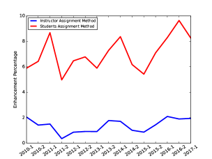
Remark 10 (Economy Perspective: Figure 2).

As it was already mentioned in the beginning of subsection 4.1, the Students Assignment method ($\mathop{}\!\mathit{SA}$) yields better results than the Instructor Assignment method ($\mathop{}\!\mathit{IA}$). This is aligned with the following idea from the economic empirical perceptions: when individuals have more instruments to participate, their well-being in terms of social welfare increases.

Academic	APV = Pass/Fail		APV = Average
Semester	$\mathop{}\!\mathit{mt}=\mathop{}\!\mathit{IA}$	$\mathop{}\!\mathit{mt}=\mathop{}\!\mathit{SA}$	$\mathop{}\!\mathit{mt}=\mathop{}\!\mathit{IA}$	$\mathop{}\!\mathit{mt}=\mathop{}\!\mathit{SA}$
2010-1	2.0482	5.8891	0.7868	1.8393
2013-1	0.9090	5.8924	0.4230	2.0870
2016-1	2.0939	8.2952	0.4391	2.1050
Mean	1.3811	7.0432	0.5501	2.1584

Table 6: Relative Enhancements Sample, $\rho_{\mathop{}\!\mathit{mt}}$, Course: Differential Calculus. We display the mean relative enhancement for the Differential Calculus course during the period from 2010-1 to 2017-1; together with a sample of three semesters in the same time window.

5 Randomization and Predictive Assessment

So far, the method has been assessed with respect to the historical log i.e., comparing its optimization outputs with those of 15 recorded semesters. The aim of the present section is to perform Monte Carlo simulations on the efficiency of the method and apply the Law of Large Numbers to estimate the expected enhancement of the algorithm. We present below for the sake of completeness, its proof and details can be found in [18].

Theorem 1 (Law of Large Numbers).

Let $\big{(}\mathrm{Z}^{(n)}:n\in\bm{\mathbbm{N}}\big{)}$ be a sequence of independent, identically distributed random variables with expectation $\mu=\mathbbm{E}(\mathrm{Z}^{(1)})$, then

$$\bm{\mathbbm{P}}\bigg{[}\Big{|}\frac{\mathrm{Z}^{(1)}+\mathrm{Z}^{(2)}+\ldots\mathrm{Z}^{(n)}}{n}-\mu\Big{|}>0\bigg{]}\xrightarrow[n\,\rightarrow\,\infty]{}0,$$ (9)

i.e. , the sequence $\big{(}\mathrm{Z}^{(n)}:n\in\bm{\mathbbm{N}}\big{)}$ converges to $\mu$ in the Cesàro sense.

In order to achieve Monte Carlo simulations, we first randomize several factors/variables which define the setting of a semester for each course, in Section 5.1. Next we discuss normalization criteria in Section 5.2, to make the enhancement simulations comparable. Finally, we present in Section 5.3, the Monte Carlo simulations results for both, the random variable simulating the benefits of the method ($\mathrm{Z}^{(n)}$ in Theorem 1) as well as the evolution of its Cesáro means ($\frac{\mathrm{Z}^{(1)}+\mathrm{Z}^{(2)}+\ldots+\mathrm{Z}^{(n)}}{n}$ in Theorem 1) to determine the asymptotic performance of the proposed algorithm.

Throughout this section we adopt a notational convention, the label RandInputAlgorithm will refer to the random versions of the respective algorithm developed in the previous sections. For instance RandInputAlgorithm 3, input: (Group Assignment Matrix G , List of Lecturers L_list , Analyzed Course, $\mathop{}\!\mathit{APV}$, Group Segmentation $\big{(}I_{\ell}:\ell\in[L]\big{)}$, $\mathop{}\!\mathit{mt}$ ), refers to Algorithm 3 above, but with a different set of input data; for clarity the randomly generated input data are underlined. This notation is introduced for exposition brevity: avoiding to write an algorithm whose logic is basically identical to its deterministic version.

5.1 Randomization of Variables

Four factors will be randomized in the same fashion: Number of Tenured Lecturers, Number of Enrolled Students, List of Students’ GPA and Number of Groups. First, we randomize the integer-valued statistical variables by merely computing 95 percent confidence intervals from the empirical data and then assuming that, the impact of the factor can be modeled by a random variable uniformly distributed on such confidence interval, see [17].

Definition 3.

Let $x$ be a scalar statistical variable with mean $\bar{x}$, standard deviation $\sigma$ and $n$ its sample size.

1. If $x$ is real-valued, its 95 percent confidence interval is given by

   $$I_{x}\overset{\textbf{def}}{=}\Big{[}\bar{x}-1.96\,\frac{\sigma}{\sqrt{n}},\bar{x}+1.96\,\frac{\sigma}{\sqrt{n}}\Big{]}.$$ (10)

2. If $x$ is integer-valued, its 95 percent confidence interval is given by

   $$I_{x}\overset{\textbf{def}}{=}\Big{[}\big{\lfloor}\bar{x}-1.96\,\frac{\sigma}{\sqrt{n}}\big{\rfloor},\big{\lceil}\bar{x}+1.96\,\frac{\sigma}{\sqrt{n}}\big{\rceil}\Big{]}\cap\bm{\mathbbm{Z}},$$ (11)

   where $x$, $\lfloor\cdot\rfloor,\lceil\cdot\rceil:\bm{\mathbbm{R}}\rightarrow\bm{\mathbbm{R}}$ denote the floor and ceiling functions respectively.

The randomization of the statistical variables listed above, heavily relies on the empirical distributions mined from the database.

Hypothesis 1.

1. Let $x$ be a scalar statistical variable, then its associated random variable $\mathrm{X}$ is uniformly distributed on its confidence interval $I_{x}$, i.e. $\mathrm{X}\sim\operatorname*{Unif}(I_{x})$, where the confidence interval is defined by (11) or (10) depending on whether the variable $x$ is integer or real valued.

2. Let $\mathbf{x}=\big{(}x_{i},\ldots,x_{d}\big{)}\in\bm{\mathbbm{R}}^{d}$ be a vector statistical variable, then its associated random variable is given by $\textbf{X}=\big{(}\mathrm{X}_{1},\ldots,\mathrm{X}_{d}\big{)}$, where $\mathrm{X}_{i}$ is the random variable associated to $x_{i}$ for all $i\in[d]$ as defined above.

From here, it is not hard to compute the confidence intervals (or ranges) of the random variables as it is shown in Tables 7 and 8. In contrast, the Sections and the GPA variables will need further considerations in its treatment.

	DC	IC	VC	VAG	LA	ODE	BM	NM
Upper Extreme	8	5	3	7	5	4	4	2
Lower Extreme	6	3	2	4	3	3	2	1
Average	7.2667	4.0667	2.6000	5.1333	3.7333	3.5333	3.3333	1.6667
Standard Deviation	0.7037	1.1629	0.7368	1.9952	1.2228	0.9155	1.0465	0.6172

Table 7: Random Variable: Number of Tenured Instructors $\mathrm{NT}$, Course: All. The upper & lower extremes, average and standard deviation for the random variable “Number of Tenure Instructors NT” across all courses are displayed.

	DC	IC	VC	VAG	LA	ODE	BM	NM
Upper Extreme	1554	1203	586	1243	1045	882	974	301
Lower Extreme	1337	1043	513	1050	932	721	837	234
Average	1445.9333	1122.8667	549.8000	1146.5333	988.6667	801.8000	905.4000	267.5333
Standard Deviation	213.4446	156.8642	70.9969	188.8304	110.7229	158.4433	134.2971	65.4847

Table 8: Random Variable: Number of Enrolled Students $\mathrm{NE}$, Course: All. The upper & lower extremes, average and standard deviation for the random variable “Number of Tenure Students NE” across all courses are displayed.

The Sections variable is a list of several sections with different capacities. A statistical scan of the data shows that this list is a most unpredictable variable, because section capacities range from 15 to 150 with very low relative frequencies in each of its values. Consequently, it was decided to group the section capacities in integer intervals

Definition 4.

Given the list of integer intervals

$$\mathcal{I}\overset{\textbf{def}}{=}\big{\{}[15,30],[31,45],[46,60],[61,75],[76,90],[91,105],[106,120],[121,135],[136,150]\big{\}},$$ (12)

for each semester and for each course, the sections frequency variable is given by

$$\mathbf{sf}\overset{\textbf{def}}{=}\Big{(}\frac{\text{ns}_{I}}{\sum\limits_{K\,\in\,\mathcal{I}}\text{ns}_{K}}:I\in\mathcal{I}\Big{)},$$ (13)

where $\text{ns}_{I}$ is the number of sections whose capacity belongs to the interval $I\in\mathcal{I}$.

Hypothesis 2.

The Sections variable S is completely defined by the number of groups variable $\mathrm{NS}$ in the following way

$$\textbf{S}\overset{\textbf{def}}{=}\Big{\lceil}\mathrm{NS}\,\overline{\mathbf{sf}}\Big{\rceil}.$$ (14)

Here $\overline{\mathbf{sf}}$ is the average vector of $\mathbf{sf}$ introduced in Equation (13) and it is understood that the ceiling function $\lceil\cdot\rceil$ applies to each component of the vector.

Finally, the GPA variable is treated as follows

Hypothesis 3.

For each semester define $\mathbf{x}\overset{\textbf{def}}{=}\big{(}x_{i}:i\in[50]\big{)}$, where $x_{i}$ is the relative frequency of registering students whose GPA is equal to $\frac{i}{10}$; in particular $\sum_{i\,\in\,[50]}x_{i}=1$. Let $\textbf{X}_{\mathop{}\!\mathit{GPA}}$ be the associated random variable to the list of relative frequencies $\mathbf{x}$, as introduced in Hypothesis 1. Then, the random variable GPA is given by

$$\textbf{GPA}\overset{\textbf{def}}{=}\big{\lceil}\mathrm{NE}\,\textbf{X}_{\mathop{}\!\mathit{GPA}}\big{\rceil},$$ (15)

where $\mathrm{NE}$ is the number of enrolled students random variable and it is understood that the ceiling function $\lceil\cdot\rceil$ applies to each component of the vector.

Remark 11.

Notice that both random variables S and GPA are the product of a scalar and a vector. However, for S the scalar is a random variable $\mathrm{NS}$ and the vector $\overline{\mathbf{sf}}$ is deterministic, while in the case of GPA the scalar $\mathrm{NE}$ and the vector $\textbf{X}_{\text{GPA}}$ are random variables. There lies the difference in the randomization of the vector variables.

So far, $\textbf{S}=\big{(}s_{K}^{(1)}:K\in\mathcal{I}\big{)}$ is producing a list of sections whose capacity lies within the ranges declared in $\mathcal{I}$ (Equation (12)), this introduces a set of slacks which will be used later on, to match the number of enrolled students $\mathrm{NE}$ with the total sections capacity. The match will be done in several steps, once the equality $\sum_{K\,\in\,\mathcal{I}}s_{K}=\mathrm{NE}$ is attained, a group assignment matrix $G$ (as in Definition 2 (i)) will be generated randomly.

1. Solve the following Data Fitting Problem (see [23] for its solution)

   Problem 3.

   Given two realizations of $\textbf{S}=\big{(}s_{K}^{(1)}:K\in\mathcal{I}\big{)}$ and $\mathrm{NE}$, consider the integer problem

   $$df^{(1)}=\min\bigg{\{}\Big{|}\sum_{K\,\in\,\mathcal{I}}\sum_{i\,=\,1}^{s_{K}^{(1)}}x_{K,i}-\mathrm{NE}\Big{|}:x_{K,i}\,\in K,\text{for all }i\in\big{[}s_{K}^{(1)}\big{]}\text{ and }K\in\mathcal{I}\bigg{\}}.$$ (16)

   Denote by $\big{(}x_{K,i}^{(1)}:i\in[s_{K}^{(1)}],K\in\mathcal{I}\big{)}$ the optimal solution to problem (16). If $df^{(1)}\equiv 0$ then jump to step 4 below.

2. Decide whether or not is more convenient increase or decrease the number of sections $s_{K}^{(1)}\mapsto s_{K}^{(2)}$ according the case, using the Greedy Algorithm 5, to modify the sections’ capacity, starting from the large sections to the small ones and get

   $$df^{(2)}\overset{\textbf{def}}{=}\Big{|}\sum_{K\,\in\,\mathcal{I}}\sum_{i\,=\,1}^{s_{K}^{(2)}}x_{K,i}^{(1)}-\mathrm{NE}\Big{|}<df^{(1)}.$$ (17)

   Data: $\big{(}s_{K}^{(1)}:K\in\mathcal{I}\big{)}$ , $\Sigma=\sum_{K\,\in\,\mathcal{I}}\sum_{i\,=\,1}^{s_{K}^{(1)}}x_{K,i}^{(1)}$, $\mathrm{NE}$.

   Result: New set of sections quantities $\big{(}s_{K}^{(2)}:K\in\mathcal{I}\big{)}$.

   Initialization;

   sort the list of intervals $\mathcal{I}$ from large values to small ones;

   if  $\Sigma>\mathrm{NE}$  then

          define $df^{(2)}\overset{\textbf{def}}{=}\Sigma-\mathrm{NE}$, $K^{(r)}\overset{\textbf{def}}{=}\text{ right extreme of }K$, for all $K\in\mathcal{I}$;

          while  $df^{(2)}>\min\{K^{(r)}:K\in\mathcal{I}\}$  do

                if  $\Sigma-\mathrm{NE}>K^{(r)}$  then

                      $s_{K}^{(2)}=s_{K}^{(1)}-1$, $df^{(2)}=df^{(2)}-K^{(r)}$

                end if

               

          end while

         

   else

          define $df^{(2)}\overset{\textbf{def}}{=}\mathrm{NE}-\Sigma$, $K^{(\ell)}\overset{\textbf{def}}{=}\text{ left extreme of }K$, for all $K\in\mathcal{I}$;

          while  $df^{(2)}>\min\{K^{(\ell)}:K\in\mathcal{I}\}$  do

                if  $\Sigma-\mathrm{NE}>K^{(\ell)}$  then

                      $s_{K}^{(2)}=s_{K}^{(1)}+1$, $df^{(2)}=df^{(1)}-K^{(\ell)}$

                end if

               

          end while

         

   end if

   Algorithm 5 Greedy Algorithm Increase/Decrease Number of Sections

   If $df^{(2)}\equiv 0$ then jump to step 4 below.

3. If $0<df^{(2)}$ (once the Greedy Algorithm 5 has been applied), apply increase/decrease capacities Algorithm 6 (breaking the constraints $x_{K,i}^{(2)}\in K$ of Equation (16)). Firstly changing $x_{K,i}^{(1)}\mapsto x_{K,i}^{(2)}$ as evenly as possible. Secondly, distributing the reminder in randomly chosen sections $x_{K,i}^{(2)}\mapsto x_{K,i}^{(3)}$ and get

   $$df^{(3)}\overset{\textbf{def}}{=}\Big{|}\sum_{K\,\in\,\mathcal{I}}\sum_{i\,=\,1}^{s_{K}^{(2)}}x_{K,i}^{(3)}-\mathrm{NE}\Big{|}\equiv 0<df^{(2)}.$$ (18)

   Data: $df^{(2)}$, $\big{(}s_{K}^{(2)}:K\in\mathcal{I}\big{)}$ , $\Sigma=\sum_{K\,\in\,\mathcal{I}}\sum_{i\,=\,1}^{s_{K}^{(2)}}x_{K,i}^{(1)}$, $\mathrm{NE}$.

   Result: New set of sections capacities $\big{(}x_{K,i}^{(2)}:i\in[s_{K}^{(2)}],K\in\mathcal{I}\big{)}$.

   initialization;

   sort the list of sections capacities $\big{(}x_{K,i}^{(1)}:i\in[s_{K}^{(2)}],K\in\mathcal{I}\big{)}$ from large values to small ones;

   define total number of sections $s\overset{\textbf{def}}{=}\sum_{K\in\mathcal{I}}s_{K}^{(2)}$;

   if  $\Sigma>\mathrm{NE}$  then

          define $u=\big{\lfloor}\dfrac{\Sigma-\mathrm{NE}}{s}\big{\rfloor}$ ;

          define $x_{K,i}^{(2)}\overset{\textbf{def}}{=}x_{K,i}^{(1)}-u$ for all $i\in[s_{K}^{(2)}],K\in\mathcal{I}$;

          choose $\Sigma-\mathrm{NE}-u\times s$ sections $K\in\mathcal{I},i\in[s_{K}^{2}]$ denote this set by $S$;

          if  $(K,i)\in S$  then

                $x_{K,i}^{(3)}\overset{\textbf{def}}{=}x_{K,i}^{(2)}-1$

         else

                $x_{K,i}^{(3)}\overset{\textbf{def}}{=}x_{K,i}^{(2)}$

          end if

         

   else

          define $u=\big{\lfloor}\dfrac{\mathrm{NE}-\Sigma}{s}\big{\rfloor}$ ;

          define $x_{K,i}^{(2)}\overset{\textbf{def}}{=}x_{K,i}^{(1)}+u$ for all $i\in[s_{K}^{(2)}],K\in\mathcal{I}$;

          choose $\mathrm{NE}-\Sigma-u\times s$ sections $K\in\mathcal{I},i\in[s_{K}^{2}]$ denote this set by $S$;

          if  $(K,i)\in S$  then

                $x_{K,i}^{(3)}\overset{\textbf{def}}{=}x_{K,i}^{(2)}+1$

         else

                $x_{K,i}^{(3)}\overset{\textbf{def}}{=}x_{K,i}^{(2)}$

          end if

         

   end if

   Algorithm 6 Greedy Algorithm Increase/Decrease Sections’ Capacity

4. Generate randomly a group assignment matrix $G$.

The random setting described above is summarized in the pseudocode 7

Data: $\mathrm{NE}$ random variable distribution, $\textbf{X}_{\mathop{}\!\mathit{GPA}}$ random variable distribution

$\mathrm{NS}$ random variable distribution, average sections frequency $\overline{\mathbf{sf}}$ variable

Analyzed Course: DC, IC, …, NM.

List of Tenured Lecturers

Result: Random Group Assignment Matrix $G$.

Initialization;

compute a realization of $\mathrm{NE}$ and a realization for $\textbf{X}_{\mathop{}\!\mathit{GPA}}$;

compute $\textbf{GPA},$ input: ($\mathrm{NE},\textbf{X}_{\mathop{}\!\mathit{GPA}}$);

call RandInputAlgorithm 1, input: (GPA list);

compute a realization of $\mathrm{NS}$ ;

compute S, input: ($\mathrm{NS},{\overline{\mathbf{sf}}}$, Analyzed Course);

solve Problem 16 input: ($\textbf{S},\mathrm{NE}$);

if  $df^{(1)}>0$  then

       run the increase/decrease number of sections Greedy Algorithm 5;

       if  $df^{(2)}>0$  then

             run the increase/decrease capacities algorithm 6 ;

             $\textbf{S}\leftarrow\big{(}x_{K,i}^{(3)}:i\in[s_{K}^{(2)}],K\in\mathcal{I}\big{)}$;

             return S

      else

            $\textbf{S}\leftarrow\big{(}x_{K,i}^{(3)}:i\in[s_{K}^{(2)}],K\in\mathcal{I}\big{)}$;

             return S

       end if

      

else

      $\textbf{S}\leftarrow\big{(}x_{K,i}^{(3)}:i\in[s_{K}^{(1)}],K\in\mathcal{I}\big{)}$;

       return S

end if

compute a random group matrix assignment $G$, input: $(\textbf{S},\textbf{GPA})$;

Algorithm 7 Random Setting Algorithm

We close this section displaying tree tables. Table 9 contains the confidence intervals for the number of sections random variable $\mathrm{NS}$. The capacities distribution vector $\overline{\mathbf{sf}}$ , as well as the confidence intervals of $\textbf{X}_{\mathop{}\!\mathit{GPA}}$ are shown in Table 10 for the course of Differential Calculus only; due to the $\mathop{}\!\mathit{GPA}$ range length, the table has been split in five rows to fit the page format. Finally, Table 12 presents an example of a group assignment matrix $G$ produced by Algorithm 7

	DC	IC	VC	VAG	LA	ODE	BM	NM
Upper Extreme	20	11	5	17	10	7	17	3
Lower Extreme	16	9	3	15	8	5	13	1
$[15,30]$	0.0202	0.0000	0.0133	0.0000	0.0000	0.0000	0.0064	0.0000
$[31,45]$	0.0030	0.0000	0.0000	0.0000	0.0000	0.0000	0.0712	0.0000
$[46,60]$	0.0403	0.0310	0.0000	0.0044	0.0000	0.0000	0.0609	0.0000
$[61,75]$	0.3802	0.0330	0.0000	0.7112	0.0572	0.0222	0.6125	0.0667
$[76,90]$	0.1155	0.0048	0.0000	0.1134	0.0083	0.0000	0.2056	0.0000
$[91,105]$	0.1034	0.0588	0.0133	0.0675	0.0763	0.0095	0.0300	0.0333
$[106,120]$	0.1640	0.2115	0.0300	0.1035	0.2939	0.0429	0.0133	0.0333
$[121,135]$	0.0629	0.3417	0.2600	0.0000	0.1791	0.3937	0.0000	0.2889
$[135,150]$	0.1104	0.3193	0.6833	0.0000	0.3852	0.5317	0.0000	0.5778

Table 9: Random Variable Number of Sections $\mathrm{NS}$ and Capacities Distribution Vector $\overline{\mathbf{sf}}$, Course: All. The upper & lower extreme and confidence intervals for the Variable number of sections $\mathrm{NS}$ are displayed for all courses.

	0.1	0.2	0.3	0.4	0.5	0.6	0.7	0.8	0.9	1.0
Upper Extreme	0.0021	0.0027	0.0031	0.0031	0.0035	0.0031	0.0044	0.0040	0.0047	0.0046
Lower Extreme	0.0012	0.0013	0.0017	0.0017	0.0024	0.0016	0.0031	0.0021	0.0020	0.0028
	1.1	1.2	1.3	1.4	1.5	1.6	1.7	1.8	1.9	2.0
Upper Extreme	0.0047	0.0045	0.0055	0.0053	0.0055	0.0056	0.0051	0.0073	0.0082	0.0084
Lower Extreme	0.0026	0.0025	0.0032	0.0028	0.0031	0.0038	0.0033	0.0049	0.0058	0.0056
	2.1	2.2	2.3	2.4	2.5	2.6	2.7	2.8	2.9	3.0
Upper Extreme	0.0114	0.0119	0.0147	0.0191	0.0208	0.0277	0.0328	0.0348	0.0420	0.0858
Lower Extreme	0.0077	0.0076	0.0105	0.0142	0.0165	0.0210	0.0250	0.0287	0.0332	0.0672
	3.1	3.2	3.3	3.4	3.5	3.6	3.7	3.8	3.9	4.0
Upper Extreme	0.0571	0.0566	0.0671	0.0668	0.0630	0.0668	0.0625	0.0527	0.0496	0.0421
Lower Extreme	0.0506	0.0489	0.0565	0.0594	0.0558	0.0549	0.0526	0.0440	0.0404	0.0357
	4.1	4.2	4.3	4.4	4.5	4.6	4.7	4.8	4.9	5.0
Upper Extreme	0.0373	0.0255	0.0209	0.0161	0.0136	0.0081	0.0055	0.0029	0.0011	0.0002
Lower Extreme	0.0282	0.0201	0.0160	0.0115	0.0088	0.0054	0.0032	0.0014	0.0002	0.0000

Table 10: Random Variable: $\textbf{X}_{\mathop{}\!\mathit{GPA}}$, Course: Differential Calculus. The distribution capacities vector $\overline{\mathbf{sf}}$ and the confidence intervals of $\textbf{X}_{\mathop{}\!\mathit{GPA}}$ for the course of Differential Calculus are displayed.

5.2 Normalization of the method and probabilistic spaces

In order to measure the proposed method’s enhancement, now there is need to normalize the results as in the case of the historical assessment of the algorithm, Section 4, Equation (8) where the improvement in the academic performance variable was divided over the historical performance of the semester at hand. In the case of Monte Carlo simulations, the concept of “historical performance” simply does not apply, as the assignation of students and/or lecturers actually did not happen. We approach this fact in two different ways

Definition 5 (Normalization Methods).

We introduce the following normalization methods.

1. Random Normalization. Normalize with respect to a random assignation of instructors or students, depending on the method IA or SA respectively.

2. Expected Normalization. Normalize with respect to the expected assignation of instructors or students, depending on the method IA or SA respectively.

In the first case, it is straightforward to compute the normalization, in the second case, the concept of expected assignation needs to be stated in neater terms. To that end, we need to present some intermediate mathematical results and definitions

Theorem 2.

Let $K\in\bm{\mathbbm{N}}$ be fixed and let $\big{(}T(i,k):i,k\in[K]\big{)}$ be a matrix. Define the Random Variable

$$\mathrm{X}_{\mathop{}\!\mathit{IA}}:\mathcal{S}_{K}\rightarrow\bm{\mathbbm{R}}, \mathrm{X}_{\mathop{}\!\mathit{IA}}(\sigma)\overset{\textbf{def}}{=}\sum\limits_{k\,\in\,[K]}T\big{(}k,\sigma(k)\big{)}.$$

Then,

$$\mathbbm{E}\big{(}\mathrm{X}_{\mathop{}\!\mathit{IA}}\big{)}=\frac{1}{K}\sum\limits_{i,k\,\in\,[K]}T(k,i)=\frac{1}{K}\,\textup{sum}(T),$$ (19)

where $\textup{sum}(T)\overset{\textbf{def}}{=}\sum\limits_{(k,i)\in[K]\times[K]}T(k,i)=\sum\limits_{k\,\in\,[K]}\sum\limits_{i\,\in[K]}T(k,i)$.

Proof.

Consider the following calculation

$$\begin{split}\mathbbm{E}\big{(}\mathrm{X}_{\mathop{}\!\mathit{IA}}\big{)}&=\frac{1}{K!}\sum\limits_{\sigma\,\in\,\mathcal{S}_{K}}\mathrm{X}_{\mathop{}\!\mathit{IA}}(\sigma)=\frac{1}{K!}\sum\limits_{\sigma\,\in\,\mathcal{S}_{K}}\sum\limits_{k\,\in\,[K]}T\big{(}k,\sigma(k)\big{)}=\frac{1}{K!}\sum\limits_{k\,\in\,[K]}\sum\limits_{\sigma\,\in\,\mathcal{S}_{K}}T\big{(}k,\sigma(k)\big{)}\\ &=\frac{1}{K!}\sum\limits_{k\,\in\,[K]}\sum\limits_{i\,\in\,[K]}\sum\limits_{\begin{subarray}{c}\sigma\,\in\,\mathcal{S}_{K}\\ \sigma(k)\,=\,i\end{subarray}}T\big{(}k,\sigma(k)\big{)}=\frac{1}{K!}\sum\limits_{k\,\in\,[K]}\sum\limits_{i\,\in\,[K]}T\big{(}k,i\big{)}\sum\limits_{\begin{subarray}{c}\sigma\,\in\,\mathcal{S}_{K}\\ \sigma(k)\,=\,i\end{subarray}}1=\frac{(K-1)!}{K!}\sum\limits_{k\,\in\,[K]}\sum\limits_{i\,\in\,[K]}T\big{(}k,i\big{)}.\end{split}$$

From here, Equation (19) follows trivially. ∎

Remark 12.

Notice that in Proposition 2 the following holds

1. It is understood that the probabilistic space is $\Omega\equiv\mathcal{S}_{K}$ where all the outcomes are equally likely.

2. Assume that the setting of a semester is given, namely: number of sections with capacities, conformation of sections and a set of instructors teaching the course. Then, $T=C_{\mathop{}\!\mathit{APV}}$, $J$ is the number of sections and $\mathbbm{E}(X_{\mathop{}\!\mathit{IA}})$ is the expected performance, when assigning instructors randomly to the available sections with defined students i.e., the $\mathop{}\!\mathit{IA}$ method.

Our next step is to be able to compute the expected performance of a group when assigning students randomly to available sections with defined instructors. This task is far more complicated due to the richness of the search space. We begin introducing some notation.

Definition 6.

Let $N,L,J\in\bm{\mathbbm{N}}$ , $\mathbf{p}=(p_{1},\ldots,p_{L})\in\bm{\mathbbm{N}}^{L},\mathbf{g}=(g_{1},\ldots,g_{J})\in\bm{\mathbbm{N}}^{J}$ be as in Definition 1.

1. Let $c:[N]\rightarrow[L]$ be the classification function of each student i.e., for each student $n\in[N]$ it assigns the label $c(n)\in[L]$ describing the profile to which he/she belongs to.

2. Define the student assignation probabilistic space by

   $$\Omega\overset{\textbf{def}}{=}\Big{\{}\omega:[N]\rightarrow[J]:\big{|}\omega^{-1}(j)\big{|}=g_{j}\,,\,\text{for all }j\in[J]\Big{\}}.$$ (20)

3. For a fixed element $\omega\in\Omega$, define the matrix $G^{\omega}\in\bm{\mathbbm{R}}^{L\times J}$ whose entries are given by

   $$G^{\omega}(\ell,j)=\big{|}\big{\{}n\in[N]:c(n)=\ell,\omega(n)=j\big{\}}\big{|}=\big{|}c^{-1}(\ell)\cap\omega^{-1}(j)\big{|}\,, \forall\,\ell\in[L],j\in[J].$$

Remark 13.

In Definition 6 notice the following

1. The student classification function satisfies that $p_{\ell}\overset{\textbf{def}}{=}\big{|}c^{-1}(\ell)\big{|}$ for all $\ell\in[L]$.

2. An element $\omega$ of the student assignation space is such that every individual is assigned to a section and every section is full (recall the sum condition (3)).

3. In our study, a list of $N$ enrolled students is completely characterized a classification function $c:[N]\rightarrow[L]$ and a section assignment function $\omega\in\Omega$

   $$\begin{array}[]{cccc}1,&2,&\ldots,&N,\\ c(1),&c(2),&\ldots,&c(N),\\ \omega(1),&\omega(2),&\ldots,&\omega(N).\end{array}$$

   The first row represents identity and the second indicates profile classification. Therefore, only the third row is subject to decision or randomization as it is done in this model.

4. For every $\omega\in\Omega$ the matrix $G^{\omega}$ is clearly a group assignment matrix as introduced in Definition 2.

Proposition 3.

Let $N,L,J\in\bm{\mathbbm{N}}$ , $\mathbf{p}=(p_{1},\ldots,p_{L})\in\bm{\mathbbm{N}}^{L},\mathbf{g}=(g_{1},\ldots,g_{J})\in\bm{\mathbbm{N}}^{J}$ be as in Definition 1. Then

$$\operatorname{trace}\big{(}T_{\mathop{}\!\mathit{APV}}G^{\omega}\big{)}=\sum\limits_{j\,=\,1}^{J}\big{(}T_{\mathop{}\!\mathit{APV}}G^{\omega}\big{)}\big{(}j,j\big{)}=\sum_{n\,\in\,[N]}T_{\mathop{}\!\mathit{APV}}\big{(}\omega(n),c(n)\big{)}, \text{for all }\omega\in\Omega.$$ (21)

Proof.

Consider the following identities

$$\begin{split}\sum_{n\,\in\,[N]}T_{APV}\big{(}\omega(n),c(n)\big{)}&=\sum_{(\ell,j)\,\in\,[L]\times[J]}\sum_{\begin{subarray}{c}n\,=\,1\\ c(n)\,=\,\ell,\,\omega(n)\,=\,j\end{subarray}}^{N}T_{APV}\big{(}\omega(n),c(n)\big{)}\\ &=\sum_{j\,\in[J]}\sum_{\ell\,\in\,[L]}T_{APV}\big{(}j,\ell\big{)}\sum_{\begin{subarray}{c}n\,=\,1\\ c(n)\,=\,\ell,\,\omega(n)\,=\,j\end{subarray}}^{N}1\\ &=\sum_{j\,\in[J]}\sum_{\ell\,\in\,[L]}T_{APV}\big{(}j,\ell\big{)}G^{\omega}(\ell,j)\\ &=\sum_{j\,\in[J]}\big{(}T_{APV}G^{\omega}\big{)}\big{(}j,j\big{)},\end{split}$$

i.e., the result holds. ∎

Remark 14.

Observe that if it is assumed that that the instructor $t_{j}$ is assigned to the section $j$ for all $j\in{J}$, i.e., the instructor assignment function $\pi\in\mathcal{S}_{J}$ of Problem 2 is the identity then, the previous result states that

$$\operatorname{trace}\big{(}T_{\mathop{}\!\mathit{APV}}G^{\omega}\big{)}=\sum\limits_{j\,=\,1}^{J}\big{(}T_{\mathop{}\!\mathit{APV}}G^{\omega}\big{)}\big{(}j,\pi(j)\big{)}=\sum_{n\,\in\,[N]}T_{\mathop{}\!\mathit{APV}}\big{(}\omega(n),c(n)\big{)},$$ (22)

for each $\omega\in\Omega$. Since the expression of the middle measures the global performance of the group, so does the right hand side. Hence, it makes sense to declare the left hand side in the expression above as a random variable.

Definition 7.

Let $N,L,J\in\bm{\mathbbm{N}}$ , $\mathbf{p}=(p_{1},\ldots,p_{L})\in\bm{\mathbbm{N}}^{L},\mathbf{g}=(g_{1},\ldots,g_{J})\in\bm{\mathbbm{N}}^{J}$ be as in Definition 1 and let $T\in\bm{\mathbbm{R}}^{J\times L}=\big{(}T(j,\ell):k\in[J],\ell\in[L]\big{)}$, be a fixed matrix. Define the student assignment performance random variable

$$\mathrm{X}_{\mathop{}\!\mathit{SA}}:\Omega\rightarrow\bm{\mathbbm{R}}\,, \mathrm{X}_{\mathop{}\!\mathit{SA}}(\omega)\overset{\textbf{def}}{=}\sum\limits_{n\,\in\,[N]}T\big{(}\omega(n),c(n)\big{)}\,.$$ (23)

Before computing the expectation of the random variable $\mathrm{X}_{\mathop{}\!\mathit{SA}}$ some previous results from combinatorics are needed.

Remark 15 (Definition 7).

The performance matrix $T$ in Definition 7 provides a measure for the performance of each instructor within each element of a given segmentation, as previously stated in Definition 2. One possible performance matrix is given by the expected performance matrix, output of the Algorithm 2 in Section 3.3. An ideal performance matrix $T$ should include more specific information about instructors as mentioned in Analysis 5 (e.g., peer ratings, self-evaluation, alumni ratings, teaching awards and others).

Lemma 4.

1. The cardinal of the student assignment space is given by

   $$|\Omega|=N!\prod\limits_{j\,=\,1}^{J}\dfrac{1}{g_{j}!}.$$ (24)

2. Let $n\in[N]$, $j\in[J]$ be fixed, and define the set

   $$\Omega_{n,j}\overset{\textbf{def}}{=}\big{\{}\omega\in\Omega:\omega(n)=j\big{\}}.$$

   Then $|\Omega_{n,j}|=\dfrac{(N-1)!}{(g_{j}-1)!}\prod\limits_{\begin{subarray}{c}i\,\in\,[K]\\ i\,\neq\,j\end{subarray}}\dfrac{1}{g_{i}!}$

Proof.

1. Let $\omega$ be an element of $\Omega$ and write it in the extended way i,e,

   $$\begin{array}[]{cccc}\omega(1),&\omega(2),&\ldots,&\omega(N),\\ 1,&2,&\ldots,&N.\end{array}$$

   Clearly, $\omega$ is a permutation of of the multiset

   $$\big{\{}\underbrace{1,1,\ldots,1}_{g_{1}\text{-times}},\underbrace{2,2,\ldots,2}_{g_{2}\text{-times}},\ldots,\underbrace{J,J,\ldots,J}_{g_{J}\text{-times}}\big{\}}=\big{\{}1\cdot g_{1},2\cdot g_{2},\ldots J\cdot g_{J}\big{\}}.$$ (25)

   From elementary combinatorics, it is known that the number of permutations of the multiset (25) is given given by the expression (24), see Theorem 3.5 in [22].

2. First we analyze the case of the set $\Omega_{N,j}$. Recalling the expression (20), we can write $\Omega_{N,j}=\big{\{}\omega:[N]\rightarrow[J]:\,\omega(N)=j,\,|\omega^{-1}(i)|=g_{i},\text{ for all }i\in[J]\big{\}}$. It is direct to see that there is a bijection with the set $\widetilde{\Omega}\overset{\textbf{def}}{=}\big{\{}\omega:[N-1]\rightarrow[J]:\big{|}\omega^{-1}(i)\big{|}=\widetilde{g}_{i}\,,\,\text{for all }i\in[J]\big{\}}$ where $\widetilde{g}_{i}$ is defined as follows

   $$\widetilde{g}_{i}\overset{\textbf{def}}{=}\begin{cases}g_{i},&i\neq j,\\ g_{i}-1,&j=i.\end{cases}$$

   Applying the previous part on the set $\widetilde{\Omega}$, it follows that $\Omega_{N,j}$ satisfies the result. For the general case $\Omega_{n,j}$, take the permutation $\sigma\in\mathcal{S}_{N}$ defined by

   $$\sigma(k)\overset{\textbf{def}}{=}\begin{cases}N,&k=n,\\ n,&k=N,\\ k&\text{otherwise}.\end{cases}$$

   Observe that the map $\varphi:\Omega_{n,j}\rightarrow\Omega_{N,j}$ defined by $\varphi(\omega)\overset{\textbf{def}}{=}\omega\circ\sigma$ is clearly a bijection. Consequently, $|\Omega_{n,j}|=|\Omega_{N,j}|$ and the proof is complete.

∎

Theorem 5.

The expectation of the random variable $\mathrm{X}_{\mathop{}\!\mathit{SA}}$ is given by

$$\mathbbm{E}\big{(}\mathrm{X}_{\mathop{}\!\mathit{SA}}\big{)}=\frac{1}{N}\,\mathbf{g}^{t}T\,\mathbf{p}.$$ (26)

Proof.

By definition

$$\begin{split}|\Omega|\,\mathbbm{E}\big{(}\mathrm{X}_{\mathop{}\!\mathit{SA}}\big{)}&=\sum\limits_{\omega\,\in\,\Omega}\sum\limits_{n\,=\,1}^{N}T\big{(}\omega(n),c(n)\big{)}=\sum\limits_{n\,=\,1}^{N}\sum\limits_{\omega\,\in\,\Omega}T\big{(}\omega(n),c(n)\big{)}\\ &=\sum\limits_{n\,=\,1}^{N}\sum\limits_{j\,=\,1}^{J}\sum\limits_{\begin{subarray}{c}\omega\,\in\,\Omega\\ \omega(n)\,=\,j\end{subarray}}T\big{(}\omega(n),c(n)\big{)}=\sum\limits_{n\,=\,1}^{N}\sum\limits_{j\,=\,1}^{J}T\big{(}j,c(n)\big{)}\sum\limits_{\begin{subarray}{c}\omega\,\in\,\Omega\\ \omega(n)\,=\,j\end{subarray}}1\end{split}$$ (27)

Recalling Lemma 4 (ii), it follows that

$$\begin{split}\mathbbm{E}\big{(}\mathrm{X}_{\mathop{}\!\mathit{SA}}\big{)}&=\frac{1}{|\Omega|}\sum\limits_{n\,=\,1}^{N}\sum\limits_{j\,=\,1}^{J}T\big{(}j,c(n)\big{)}\dfrac{(N-1)!}{(g_{j}-1)!}\prod\limits_{\begin{subarray}{c}i\,\in\,[J]\\ i\,\neq\,j\end{subarray}}\dfrac{1}{g_{i}!}\\ &=\frac{1}{|\Omega|}\sum\limits_{n\,=\,1}^{N}\sum\limits_{j\,=\,1}^{J}g_{j}\,T\big{(}j,c(n)\big{)}(N-1)!\prod\limits_{i\,\in\,[J]}\dfrac{1}{g_{i}!}=\frac{1}{N}\sum\limits_{j\,=\,1}^{J}\sum\limits_{n\,=\,1}^{N}g_{j}\,T\big{(}j,c(n)\big{)}\\ &=\frac{1}{N}\sum\limits_{j\,=\,1}^{J}g_{j}\sum_{\ell\,=\,1}^{L}\sum\limits_{\begin{subarray}{c}n\,\in\,[N]\\ c(n)\,=\,\ell\end{subarray}}\,T\big{(}j,c(n)\big{)}=\frac{1}{N}\sum\limits_{j\,=\,1}^{J}g_{j}\sum_{\ell\,=\,1}^{L}T\big{(}j,\ell\big{)}p_{\ell}\\ &=\frac{1}{N}\sum_{\ell\,=\,1}^{L}p_{\ell}\sum\limits_{j\,=\,1}^{J}T\big{(}j,\ell\big{)}g_{j}.\end{split}$$ (28)

Here, the second equality uses the identity $\frac{1}{(g_{j}-1)!}=\frac{g_{j}}{g_{j}!}$ and the third uses the expression (24), together with an obvious exchange of indexes. The fourth equality is a convenient association of summands, while the fifth merely uses the fact $|c^{-1}(\ell)|=p_{\ell}$. From here, the result follows trivially. ∎

Remark 16.

Let $\pi\in\mathcal{S}_{J}$ be a permutation and let $A^{\pi}$ its associated permutation matrix

$$A^{\pi}=\big{[}\mathbf{\widehat{e}}_{\pi(1)},\mathbf{\widehat{e}}_{\pi(2)},\ldots,\mathbf{\widehat{e}}_{\pi(J)}\big{]},$$

where $\big{(}\mathbf{\widehat{e}}_{j}:j\in[J]\big{)}$ is the canonical basis of $\bm{\mathbbm{R}}^{J}$. Then, if the instructors $\big{\{}t_{j}:j\in[J]\big{\}}$ are assigned to their corresponding sections by a permutation $\pi\in\mathcal{S}_{J}$, other than the identity, by taking

$$T\overset{\textbf{def}}{=}T_{\mathop{}\!\mathit{APV}}\,A^{\pi},$$

the random variable $\mathrm{X}_{\mathop{}\!\mathit{SA}}(\omega)$ (as defined in (23)), computes the global performance of the group for each $\omega\in\Omega$ (as discussed in Remark 14). Therefore, without loss of generality, it can be assumed that $\pi\in\mathcal{S}_{J}$ is the identity.

Finally we define

Definition 8.

The random version of Algorithm 3 will have two methods.

1. The Random Normalization method introduced in Definition 5 a defined in Equation 8. However, it is important to observe that this time $v_{\mathop{}\!\mathit{mt}}$, $\rho_{\mathop{}\!\mathit{mt}}$ and $\mathrm{X}_{\mathop{}\!\mathit{mt}}\overset{\textbf{def}}{=}\sum_{j\,=\,1}^{J}\big{(}T_{APV}G_{h}\big{)}\big{(}j,\pi_{h}(j)\big{)}$ are all random variables.

2. Second, the Expected Normalization method introduced in Definition 5 b, which is computed using

   $$\gamma_{\mathop{}\!\mathit{mt}}\overset{\textbf{def}}{=}100\frac{v_{\mathop{}\!\mathit{mt}}-\mathbbm{E}\big{(}\mathrm{X}_{\mathop{}\!\mathit{mt}}\big{)}}{\mathbbm{E}\big{(}\mathrm{X}_{\mathop{}\!\mathit{mt}}\big{)}}\,, \mathop{}\!\mathit{mt}\in\{\mathop{}\!\mathit{IA},\mathop{}\!\mathit{SA}\}.$$ (29)

   Here, $\mathbbm{E}\big{(}\mathrm{X}_{\mathop{}\!\mathit{mt}}\big{)}$ is given by Theorem 2 if $\mathop{}\!\mathit{mt}=\mathop{}\!\mathit{IA}$ and by Theorem 5 if $\mathop{}\!\mathit{mt}=\mathop{}\!\mathit{SA}$. Again, $v_{\mathop{}\!\mathit{mt}}$ and $\gamma_{\mathop{}\!\mathit{mt}}$ are both random variables.

Remark 17.

1. It is understood that, for the application of the Law of Large Numbers 1 in the numerical experiments, the random variables above will be considered as sequences of independent, identically distributed, variables i.e., $\big{(}v_{\mathop{}\!\mathit{mt}}^{(n)}:n\in\bm{\mathbbm{N}}\big{)}$, $\big{(}\mathrm{X}_{\mathop{}\!\mathit{mt}}^{(n)}:n\in\bm{\mathbbm{N}}\big{)}$, $\big{(}\rho_{\mathop{}\!\mathit{mt}}^{(n)}:n\in\bm{\mathbbm{N}}\big{)}$ and $\big{(}\gamma_{\mathop{}\!\mathit{mt}}^{(n)}:n\in\bm{\mathbbm{N}}\big{)}$; where the index $n$ indicates an iteration of the Monte Carlo simulation.

2. It is direct to see that $\big{(}\gamma_{\mathop{}\!\mathit{mt}}^{(n)}:n\in\bm{\mathbbm{N}}\big{)}$ converges in the Cesàro sense to $\mathbbm{E}\big{(}v_{\mathop{}\!\mathit{mt}}^{(1)}\big{)}\big{(}\mathbbm{E}\big{(}\mathrm{X}_{\mathop{}\!\mathit{mt}}^{(n)}\big{)}\big{)}^{-1}-1$.

3. Define $\mathrm{Z}_{\mathop{}\!\mathit{mt}}^{(n)}\overset{\textbf{def}}{=}\dfrac{1}{\mathrm{X}_{\mathop{}\!\mathit{mt}}^{(n)}}$, since $\big{(}v_{\mathop{}\!\mathit{mt}}^{(n)}:n\in\bm{\mathbbm{N}}\big{)}$ and $\big{(}\mathrm{X}_{\mathop{}\!\mathit{mt}}^{(n)}:n\in\bm{\mathbbm{N}}\big{)}$ are independent, it holds that

   $$\rho_{\mathop{}\!\mathit{mt}}^{(n)}=\frac{v_{\mathop{}\!\mathit{mt}}^{(n)}-\mathrm{X}_{\mathop{}\!\mathit{mt}}^{(n)}}{\mathrm{X}_{\mathop{}\!\mathit{mt}}^{(n)}}=\frac{v_{\mathop{}\!\mathit{mt}}^{(n)}}{\mathrm{X}_{\mathop{}\!\mathit{mt}}^{(n)}}-1=v_{\mathop{}\!\mathit{mt}}^{(n)}\mathrm{Z}_{\mathop{}\!\mathit{mt}}^{(n)}-1\xrightarrow[n\,\rightarrow\,\infty]{\text{Ces\`{a}ro}}\mathbbm{E}\big{(}v_{\mathop{}\!\mathit{mt}}^{(1)}\big{)}\mathbbm{E}\big{(}\mathrm{Z}_{\mathop{}\!\mathit{mt}}^{(n)}\big{)}-1=\mathbbm{E}\big{(}v_{\mathop{}\!\mathit{mt}}^{(1)}\big{)}\mathbbm{E}\Big{(}\frac{1}{\mathrm{X}_{\mathop{}\!\mathit{mt}}^{(n)}}\Big{)}-1.$$ (30)

   The right hand side of the expression above involves the reciprocal of the harmonic mean of the variable $\big{(}\mathrm{X}_{\mathop{}\!\mathit{mt}}^{(n)}:n\in\bm{\mathbbm{N}}\big{)}$. Clearly, $\big{(}\gamma_{\mathop{}\!\mathit{mt}}^{(n)}:n\in\bm{\mathbbm{N}}\big{)}$ and $\big{(}\rho_{\mathop{}\!\mathit{mt}}^{(n)}:n\in\bm{\mathbbm{N}}\big{)}$ converge (in the Cèsaro sense) to different limits. Unfortunately, the harmonic mean has no simple expression equivalent to that of Equation (26) for the arithmetic mean. Consequently, it can be handled only numerically; this will be done in the next section.

5.3 The Monte Carlo Simulation Algorithm and Numerical Results

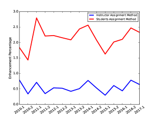
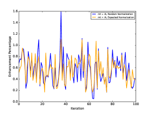
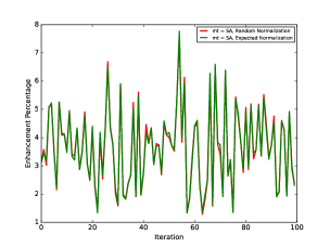
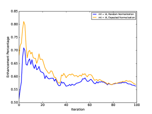
The randomization of the variables as well as its normalization discussed in the sections 5.1 and 5.2 respectively are summarized in the pseudocode 8 below. A particular example of the Monte Carlo simulation results is depicted in Figure 3, while the corresponding body/composition of enrolled students displayed presented in Table 12.

The results of several simulations for the Differential Calculus course are summarized in Table 11. Out several experiments, it is observed that a reasonable level of convergence of the Cesàro means is attained above 800 iterations. Given that we are simulating the behavior of a highly complex random process, it is clear that no convergence rate can actually be concluded, the threshold for which the Cesàro mean stabilizes shifts significantly from one experiment to the other. This is because every experiment defines a number of sections $\mathrm{NS}$, an enrollment body/composition of students as in Table 12, a group matrix assignment $G$ and a number of tenured lecturers $\mathrm{NT}$, from here, the iteration process begins as it is shown in Algorithm 8. Therefore, the starting triple $(\mathrm{NS},G,\mathrm{NT})$ changes substantially between simulations as it can be seen in Table 11. These changes become even more dramatical when shifting from one course to another, as it is the case of Table 13, reporting the algorithm’s performance for all the remaining seven service courses.

It is also important to observe the difference between Random (Definition 5 a) vs. Expected (Definition 5 b) normalization methods. It is not significant in the simulation of the method’s performance (see Figure 3 (a) and (b)) and it is negligible in the behavior of their corresponding Cesàro means, i.e., regardless of the chosen normalization method (see figure Figure 3 (c) and (d)), the asymptotic behavior difference is negligible at least, from the numerical point of view. The latter can be also observed on the Tables 11 and 13.

Remark 18 (Figure 3).

Figure 3 depicts enhancement (and Cesàro means enhancement) results for the variable Pass Rate of the Monte Carlo Simulation, for both: the Instructor and the Student Assignment Methods. It confirms the result from Subsection 4.1, the Students Assignment Method ($\mathop{}\!\mathit{SA}$) yields better results than the Instructor Assignment Method ($\mathop{}\!\mathit{IA}$), and it shows that this result is not merely a particularity from our data set. Instead, it constitutes a robust one.

Experiment	Random Normalization, $\rho_{\mathop{}\!\mathit{mt}}$		Expected Normalization, $\gamma_{\mathop{}\!\mathit{mt}}$		Enrollment	Sections	Lecturers
Number	$100\times\dfrac{v_{\mathop{}\!\mathit{IA}}}{\rho_{\mathop{}\!\mathit{IA}}}$	$100\times\dfrac{v_{\mathop{}\!\mathit{SA}}}{\rho_{\mathop{}\!\mathit{SA}}}$	$100\times\dfrac{v_{\mathop{}\!\mathit{IA}}}{\gamma_{\mathop{}\!\mathit{IA}}}$	$100\times\dfrac{v_{\mathop{}\!\mathit{SA}}}{\gamma_{\mathop{}\!\mathit{SA}}}$	$\mathrm{NS}$	$\sum\limits_{K\,\in\,\mathcal{I}}s_{K}$	$\mathrm{NT}$
1	0.3097	2.9059	0.3056	2.9044	1355	15	6
2	0.4595	3.2880	0.4588	3.2854	1445	14	8
3	0.4373	3.2655	0.4414	3.2653	1225	14	7
4	0.4158	3.2689	0.4130	3.2663	1456	15	7
5	0.4357	2.9680	0.4315	2.9651	1296	14	6
6	0.4943	3.1690	0.5053	3.1697	1547	15	8
7	0.5099	3.4486	0.5008	3.4439	1556	16	8
8	0.4937	3.3720	0.4841	3.3666	1532	16	8
9	0.4080	3.1254	0.4009	3.1301	1444	15	7
10	0.4843	3.4498	0.4807	3.4454	1546	16	8
Mean	0.4448	3.2261	0.4422	3.2242	1440.2	15.0	7.3

Table 11: Monte Carlo Simulations Summary. The table shows a summary of the Monte Carlo Simulations with 10 experiments and 800 iterations each, for the Differential Calculus course.

Data: Database: Assembled_Data.csv Analyzed Course: DC, IC, …, NM.

Optimization Method: $\mathop{}\!\mathit{mt}\in\{\mathop{}\!\mathit{IA},\mathop{}\!\mathit{SA}\}$.

$\mathrm{NT}$ random variable distribution

Numer of Iterations: $NI$

Result: Table of Relative Enhancement Values $\rho_{\mathop{}\!\mathit{mt}}$, $\gamma_{\mathop{}\!\mathit{mt}}$ for chosen method, course and academic performance variable.

Initialization;

call Algorithm 7;

$\mathit{nt}\leftarrow$compute a realization of $\mathrm{NT}$;

call Algorithm 2, input: (Assembled_Data.csv, Analyzed Course, $\mathop{}\!\mathit{APV}$, Group Segmentation $\big{(}I_{\ell}:\ell\in[L]\big{)}$);

for  iteration $\in[NI]$  do

       $\mathit{list}\leftarrow$ compute a random list of $nt$-lecturers;

       call RandInputAlgorithm 3, input: (Group Assignment Matrix G , List of Lecturers L_list , Analyzed Course, $\mathop{}\!\mathit{APV}$, Group Segmentation $\big{(}I_{\ell}:\ell\in[L]\big{)}$, $\mathop{}\!\mathit{mt}$ );

      

      APV_mt_Assessment[iteration]$\leftarrow\big{[}\rho_{\mathop{}\!\mathit{mt}},\gamma_{\mathop{}\!\mathit{mt}}\big{]}$.

end for

Algorithm 8 Monte Carlo Simulation Algorithm

(a) Example DC. Enhancement Results Pass Rate Monte Carlo Simulation. Instructor Assignment Method ($\mathop{}\!\mathit{IA}$).

(b) Example DC. Enhancement Results Pass Rate Monte Carlo Simulation. Student Assignment Method ($\mathop{}\!\mathit{SA}$).

(c) Example DC. Cesàro Means Enhancement Results Pass Rate Monte Carlo Simulation. Instructor Assignment Method ($\mathop{}\!\mathit{IA}$).

(d) Example DC. Cesàro Means Enhancement Results Pass Rate Monte Carlo Simulation. Student Assignment Method ($\mathop{}\!\mathit{SA}$).

Figure 3: Example: Differential Calculus course. Enrollment of 1441 Students, 15 Sections, 8 Tenured Lecturers, 100 Iterations. All figures display the normalization $\rho_{\mathop{}\!\mathit{mt}}$ vs $\gamma_{\mathop{}\!\mathit{mt}}$ for $\mathop{}\!\mathit{mt}\in\{\mathop{}\!\mathit{IA},\mathop{}\!\mathit{SA}\}$.

	[0, 2.2]	(2.2, 2.7]	(2.7, 3.0]	(3.0, 3.1]	(3.1, 3.3]	(3.3, 3.5]	(3.5, 3.7]	(3.7, 3.8]	(3.8, 4.1]	(4.1, 5.0]	Total
1	6	1	15	5	13	8	8	4	8	6	74
2	10	6	14	3	5	7	11	5	8	5	74
3	9	9	9	8	6	3	9	1	15	5	74
4	11	12	13	1	5	3	8	7	8	6	74
5	5	9	12	7	11	6	9	2	5	9	75
6	9	7	6	3	13	11	11	1	7	6	74
7	12	5	7	2	7	10	12	6	21	7	89
8	7	11	11	2	6	12	14	8	9	9	89
9	11	18	14	7	6	12	10	7	10	9	104
10	7	9	15	7	14	14	16	8	8	6	104
11	14	8	20	4	15	17	14	0	13	14	119
12	7	11	14	6	13	21	14	4	18	11	119
13	15	15	15	9	15	16	11	3	11	9	119
14	14	14	20	5	17	15	12	4	9	9	119
16	15	13	25	6	15	16	10	9	17	8	134
Total	152	148	210	75	161	171	169	69	167	119	1441

Table 12: An example of a random realization of Algorithm 7, i.e. a group matrix assignment $G$ and a number of tenured lecturers $\mathrm{NT}$ for the Differential Calculus course.

Course	Random Normalization, $\rho_{\mathop{}\!\mathit{mt}}$		Expected Normalization, $\gamma_{\mathop{}\!\mathit{mt}}$		Enrollment	Sections	Lecturers
	$100\times\dfrac{v_{\mathop{}\!\mathit{IA}}}{\rho_{\mathop{}\!\mathit{IA}}}$	$100\times\dfrac{v_{\mathop{}\!\mathit{SA}}}{\rho_{\mathop{}\!\mathit{SA}}}$	$100\times\dfrac{v_{\mathop{}\!\mathit{IA}}}{\gamma_{\mathop{}\!\mathit{IA}}}$	$100\times\dfrac{v_{\mathop{}\!\mathit{SA}}}{\gamma_{\mathop{}\!\mathit{SA}}}$	$\mathrm{NS}$	$\sum\limits_{K\,\in\,\mathcal{I}}s_{K}$	$\mathrm{NT}$
DC	0.4448	3.2261	0.4422	3.2242	1440.2	15.0	7.3
IC	0.3267	2.8094	0.3196	2.8104	1068.0	8.2	5.1
VC	0.1684	1.9797	0.1800	1.9923	586.6	4.1	2.4
VAG	0.4070	3.1366	0.4079	3.1474	1080.8	14.5	6.2
LA	0.2131	3.2906	0.2009	3.2788	1078.2	8.0	4.2
ODE	0.4323	5.6270	0.4269	5.6332	798.2	6.4	3.1
BM	0.5706	3.0775	0.5909	3.0791	910.9	11.1	3.0
NM	0.3750	3.3825	0.3405	3.3920	263.1	2.3	1.7

Table 13: A summary of the Monte Carlo Simulations with 800 iterations for each course.

6 Conclusions and Future Work

The present work delivers several conclusions.

1. From the modeling point of view

   1. A method has been implemented aimed to increase the academic performance for massive university lower division courses in mathematics. It is based on integer programming and big data analysis to compute the associated cost functions, while the constraints (such as the number of sections and corresponding capacities) are defined by administrative sources. The integer programs come from two mechanisms: assign instructors optimally ($\mathop{}\!\mathit{IA}$ method) or assign students optimally ($\mathop{}\!\mathit{SA}$ method).

   2. The academic performance was explored using two measures; Pass Rate and Grade. After correlation analysis of the data, it is determined that the one relevant factor, known at the time when the semester begins and incident on these statistical variables is the $\mathop{}\!\mathit{GPA}$. Consequently the profiling of students as well as the student body composition is defined in terms of the $\mathop{}\!\mathit{GPA}$ (see Table 6)

   3. The historical assessment of the method yields poor enhancement levels for the Grade variable, due to its typical statistical robustness. However, the Pass Rate yields more satisfactory results; good enough to pursue a deeper analysis such as the method’s randomization and its asymptotic assessment, presented in Section 5.

   4. The asymptotic analysis of the algorithm is done by randomizing the enrollment population and the administrative factors, statistically based on the empirical observations reported in the database Assembled_Data.csv. The Monte Carlo experiments establish that the method does not deliver a fixed value of relative enhancement, it depends on the starting parameters $\big{(}\mathrm{NS},G,\mathrm{NT}\big{)}$ whose remarkable randomness inherit uncertainty to the algorithm’s output values.

   5. Computing a weighted average across the courses by crossing the tables 8 and 13, gives a rough estimate of 3.3 percent full scale benefit, if the students assignment method ($\mathop{}\!\mathit{SA}$) is implemented. This is approximately 240 extra students per semester passing their respective courses which, in the long run represent a significant gain for the Institution.

   6. The algorithms 4 and 8, could have been adjusted to keep only the sections with tenured lecturers. However, the Authors chose to discard this artificial setting because it is biased with respect to the study case.

   7. It is the perception of the Authors that no general conclusions can be derived for the method’s enhancement level. On one hand it is sufficiently general and flexible to be implemented at any Institution with massive courses and therefore big databases available. On the other hand, the experiments performed in the present work, suggest that its effectiveness needs to be evaluated on a case-wise basis.

   8. Considering age as a factor is also possible by merely applying the segmentation process described in Section 3.2 (Algorithm 1 with an adequate number of segmentation intervals $\big{(}\widetilde{I}_{\ell}:\ell\in[\widetilde{L}]\big{)}$). First, computing the lecturers performance conditioned to the Age variable as in Section 3.3 (Algorithm 2, output $T_{\textit{Age}}$). Second, weighting its impact according to the correlation values, namely the costs table in Equation (5) can be modified as

      $$C=\frac{4}{5}\,T_{\textit{APV}}G+\frac{1}{5}T_{\textit{Age}}\widetilde{G}.$$ (31)

      Here it is understood that the group matrix $\widetilde{G}$ is constructed according to the Age variable segmentation $\big{(}\widetilde{I}_{\ell}:\ell\in[\widetilde{L}]\big{)}$. The weighting coefficients were proposed, according to the correlation with the Grade variable reported in Table 2: Age: 0.2, $\mathop{}\!\mathit{GPA}$: 0.8, i.e., the second is 4 times the first one (see [8] for further discussion on these type of models). Yet again, the flexibility of the method, allows to introduce in the same fashion any number of variables fitting to the case at hand.

2. From the economy point of view

   1. A 3.3 % enhancement for the method’s benefit may seem low at first sight. However, it is important to stress that this enhancement corresponds to a detailed treatment of the tenured lecturers only, while the adjunct lecturers are treated in general terms because of insufficient data as they are unstable personnel. Tenured lecturers represent a fraction of less than 50 percent from the involved faculty team as Table 13 shows. Consequently, should the stable personnel fraction increase, the method would deliver more accurate and perhaps more optimistic results.

   2. The method presented in this work offers a mechanism for higher education institutions to help their students improving their pass rates and grades. This is done by solving two different social welfare schedules ($\mathop{}\!\mathit{IA}$ and $\mathop{}\!\mathit{SA}$ methods). Under this approach, the University is considered as an agent that provides education, and as a rational regulator agent, capable to optimally allocate some of its resources for enhancement of social welfare of its students body.

   3. The method has two important features that are particularly relevant in countries like Colombia where the drop out rates from college are high and the investment in higher education is low: $\bullet$ By helping students to improve their pass rates and grades, it is alleviating the problem of high drop out rates; $\bullet$ the method does not require major money investment from the University in order to be implemented. In theory, only the data and a capable person are required to implement it.

   4. The work also provides a way to measure (and monitor) how far from the Pareto equilibrium is an Institution at a given time. This important because it provides a way to determine whether the expected enhancement results are being achieved or not.

3. From the future work point of view

   1. This paper has worked two methods, assign instructors while keeping the students fixed ($\mathop{}\!\mathit{IA}$) and assign students while keeping the instructors fixed ($\mathop{}\!\mathit{SA}$), both of them come down to a linear optimization problem, 1 and 2 respectively. However, moving both instructors and students simultaneously is no longer a linear, but a bilinear optimization question (see [24, 25]). This view will be further explored in future work.

   2. So far, the present work assumed that allocating students and/or instructors is a decision centralized by the administrative departments of the analyzed Institution. However, in our study case, student location is decided differently, using a $\mathop{}\!\mathit{GPA}$ competition-based mechanism to assign priority starting from the highest to the lowest scorers. This competitive scenario is better modeled using game theory which will be explored in future work.

   3. The algorithm presented in this work offers a mechanism for higher education institutions to help their students improving their pass rates and grades. This is done by solving two different social welfare schedules ($\mathop{}\!\mathit{IA}$ and $\mathop{}\!\mathit{SA}$ methods). The work also provides a way to measure (and monitor) how far from the Pareto equilibrium is an Institution at a given time. As mentioned in the economic justification (Subsection 1.1), this is particularly relevant in countries like Colombia where the drop out rates from college are high.

7 Acknowledgements

The Authors wish to thank Universidad Nacional de Colombia, Sede Medellín for its support in the production of this work, in particular, to the Academic Director of the University for allowing access to their databases for this study. The first author was supported by grant Hermes 45713 from Universidad Nacional de Colombia, Sede Medellín.

References

- [1] J. Theroux, Real-time case method: analysis of a second implementation, Journal of Education for Business July/August (2009) 367–373.
- [2] F. Castro, A. Bellido, A. Netbo, F. Mugica, Applying data mining techniques to e-learning problems, Studies in Computational Intelligence 62 (2007) 183–221.
- [3] J. Beck, J. Mostow, How who should practice; using learning decomposition to evaluate the efficacy of different types for different types of students, Proceedings of the 9th International Conference on Intelligent Tutoring Systems (2008) 353–362.
- [4] S. Levy, I. Wilensky, Mining students’ inquiry actions for understanding of complex systems, Computers & Education 56 (2011) 556–573.
- [5] L. Herrenkohl, T. Tasker, Pedagogical practices to support classroom cultures of scientific inquiry, Cognition and Instruction 29 (1) (2011) 1–44.
- [6] L. Maacfayden, S. Dawson, Mining L.M.S. data to develop an “Early warning system for educators”, Computers & Education 54 (2010) 588–599.
- [7] E. Lazear, Educational production, The Quarterly Journal of Economics 116 (3) (2001) 777–803.
- [8] G. De Giorgi, M. Pellizzari, W. G. Woolston, Class size and heterogeneity, Journal of the European Economic Association 10 (4) (2012) 795–830.
- [9] G. De Giorgi, M. Pellizzari, S. Redaelli, Identification of social interactions through partially overlapping peer groups, American Economical Journal: Applied Economics 2 (2) (2010) 241–75.
- [10] A. B. Kruegger, Experimental estimates of educacton production functions, The Quarterly Journal of Economics 114 (42) (2009) 497–532.
- [11] G. Grace, Education: commodity or public good?, British Journal of Educational Studies 37 (3) (1989) 207–221.
- [12] J. B. Tilak, Higher education: a public good or a commodity for trade?, Prospects 38 (4) (2008) 449–466.
- [13] J. Londono-Velez, C. Rodriguez, F. Sánchez, The intended and unintended impacts of a merit-based financial aid program for the poor: The case of ser pilo paga, Documento CEDE (2017-24) (2017).
- [14] M. Marta Ferreyra, C. Avitabile, J. Botero Álvarez, F. Haimovich Paz, S. Urzúa, At a crossroads: higher education in Latin America and the Caribbean, The World Bank, 2017.
- [15] J. D. Angrist, V. Lavy, Using Maimonides rule to estimate the effect of class size on scholastic achievement, The Quarterly Journal of Economics 114 (2) (2012) 533–575.
- [16] C. M. Hoxby, The effects of class size on student achievement: New evidence from population variation, The Quarterly Journal of Economics 115 (4) (2000) 1239–1285.
- [17] W. I. Mendenhall, R. J. Beaver, B. M. Beaver, Introduction to Probability and Statistics, 14th Edition, Wiley Series in Probability and Mathematical Statistics, Brooks/Cole, Cengage Learning, Boston, MA, 2013.
- [18] P. Billinsgley, Probability and Measure, Wiley Series in Probability and Mathematical Statistics, John Wiley Sons, Inc., New York, 1995.
- [19] J. Higgins, Performance measurement in universities, European journal of operational research 38 (3) (1989) 358–368.
- [20] J. E. Rockoff, C. Speroni, Subjective and objective evaluations of teacher effectiveness, American Economic Review 100 (2) (2010) 261–66.
- [21] R. A. Berk, Survey of 12 strategies to measure teaching effectiveness, International journal of teaching and learning in higher education 17 (1) (2005) 48–62.
- [22] M. Bóna, A Walk Through Combinatorics, 3rd Edition, World Scientific, Singapore, 2011.
- [23] D. Bertsimas, J. N. Tritsiklis, Introduction to Linear Optimization, Athena Scientific and Dynamic Ideas, LLC, Belmont, MA, 1997.
- [24] A. V. Orlov, Numerical solution of bilinear programming problems, Computational Mathematics and Mathematical Physics 48 (2) (2008) 225–241.
- [25] A. Caprara, M. Monaci, Bidimensional packing by bilinear programming, Mathematical Programming 118 (2009) 225–241.